Integration of Lean Analytics and Industry 6.0: A Novel Meta-Theoretical Framework for Antifragile, Generative AI-Orchestrated, Circular–Regenerative, and Hyper-Connected Manufacturing Ecosystems

Abstract

The convergence of Lean manufacturing principles with Industry 4.0 has yielded significant operational improvements, yet the emerging paradigm of Industry 6.0—characterized by antifragile, autonomous, and sustainable systems—demands a fundamental rethinking of existing analytical frameworks. This paper introduces the Industry 6.0 Lean Analytics (I6LA) Framework, a novel meta-theoretical approach that integrates Lean principles with the core concepts of Industry 6.0. By systematically analyzing the limitations of current Lean analytics in the context of Industry 6.0 requirements, we identify critical gaps in areas such as system resilience, AI-driven autonomy, and circular economy integration. The I6LA Framework addresses these gaps through four new theoretical pillars: Antifragile Lean Systems Theory, generative AI-Orchestrated Value Streams, Circular–Regenerative Analytics, and Hyper-Connected Ecosystem Integration. This research provides a new set of mathematical models for measuring antifragility, generative orchestration efficiency, and circularity, offering a comprehensive analytical toolkit for the next generation of manufacturing. The framework’s primary contribution is a paradigm shift from optimizing stable, human-in-the-loop systems to managing dynamic, autonomous ecosystems that thrive on volatility and are regenerative by design. This paper provides both a robust theoretical foundation and practical implementation guidance for organizations navigating the transition to Industry 6.0.

1. Introduction

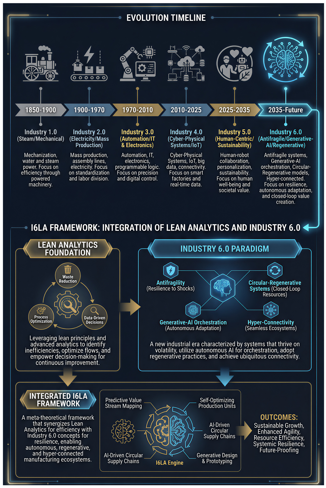
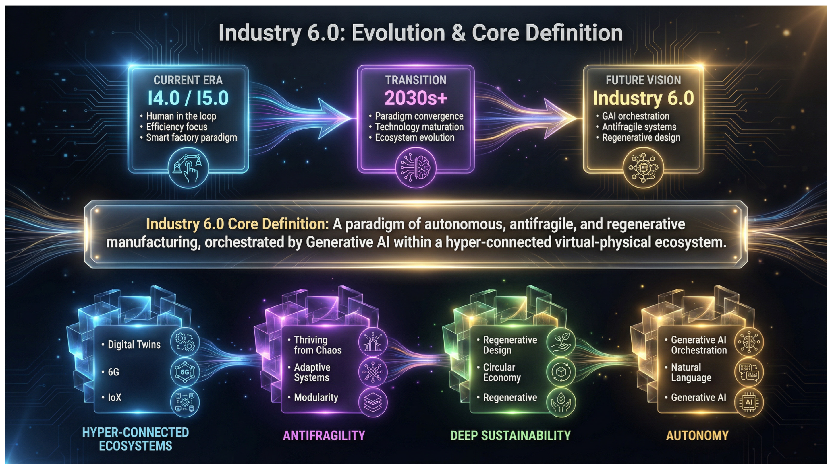
The transition from conventional manufacturing to the integrated and interconnected Cyber–Physical Systems (CPS) frameworks of Industry 4.0 (I4.0) and the Human–AI Interaction (HAII) frameworks of Industry 5.0 (I5.0) has resulted in a notable enhancement in operational efficiency and data-informed decision-making (see Figure 1). The use of Lean concepts in the I4.0/I5.0 framework, commonly referred to as “Digital Lean,” has allowed firms to attain unparalleled levels of waste minimization and process enhancement. Nevertheless, the industrial landscape is poised for a significant transformation: the advent of Industry 6.0 (I6.0). This forthcoming wave is not only a marginal enhancement of Industry 4.0/5.0 but signifies a major paradigm change towards manufacturing systems that are autonomous, antifragile, sustainable, and intricately connected with virtual–physical ecosystems [1].

I6.0 anticipates a future in which manufacturing is defined by omnipresent, customer-centric, and virtualized operations that are not only resilient to disruptions but also antifragile, able to learn and enhance from such experiences (see Figure 2). This new epoch will be propelled by technologies including generative AI (GAI), quantum computing, 6G networks, and the Internet of Anything (IoX), establishing a hyper-connected milieu whereby autonomous AI agents coordinate whole value streams. Moreover, I6.0 prioritizes sustainability and circularity, requiring industrial processes to align with environmental limits and facilitate ecological regeneration [2].

This forthcoming transition reveals the significant shortcomings of existing Lean manufacturing analytics. Current frameworks, tailored for the stable and human-centered contexts of Industry 4.0 and 5.0, are inadequate for addressing the complexity, autonomy, and volatility inherent in I6.0 systems. The conventional emphasis on waste elimination in predictable processes is inadequate for a world where systems must flourish amidst unpredictability. Contemporary human-in-the-loop optimization methods are insufficient for governing the emerging, self-organizing behavior of GAI-driven ecosystems. The independent “green” initiatives of contemporary Lean procedures inadequately fulfill the profound, real-time integration of circular economy principles required by I6.0 [3].

This paper presents the Industry 6.0 Lean Analytics (I6LA) framework, a novel meta-theoretical approach aimed at establishing the analytical foundations for Lean manufacturing in the context of Industry 6.0. The I6LA framework signifies a transition from optimizing stable, predictable systems to overseeing dynamic, autonomous, and regenerative ecosystems. It offers an extensive toolkit for assessing, analyzing, and enhancing the performance of manufacturing systems that are Antifragile, GAI-Orchestrated, and inherently circular.

The primary contribution of this research is the development of a new theoretical framework that bridges the gap between traditional Lean principles and the transformative requirements of I6.0. The I6LA framework is built upon four new theoretical pillars:

• Antifragile Lean Systems Theory: Extends Lean’s focus from stability and robustness to antifragility, providing models for systems that gain strength from disorder.
• GAI-Orchestrated Value Streams: Shifts the analytical focus from human-driven optimization to the management and optimization of autonomous, GAI-driven value stream orchestration.
• Circular–Regenerative Analytics: Integrates circular economy and regenerative design principles into the core of Lean performance measurement, moving beyond simple sustainability metrics.
• Hyper-Connected Ecosystem Integration: Provides analytical tools for optimizing information flow and performance across vast, interconnected virtual–physical ecosystems.

This paper presents the complete I6LA framework, including its theoretical underpinnings, a new set of mathematical models for measuring performance in I6.0 environments, and a practical methodology for implementation. By providing a robust and comprehensive analytical foundation for the future of manufacturing, this research offers a critical resource for academics, practitioners, and policymakers navigating the transition to I6.0.

2. The Path to I6.0

A comprehensive understanding of the I6LA framework requires a thorough examination of the literature that defines the evolution from Industry 4.0 to Industry 6.0. This review synthesizes the key concepts from the provided foundational papers, organizing them into a coherent narrative that establishes the theoretical basis for our proposed framework.

2.1. I4.0: The Digital Foundation

I4.0, initially conceived in Germany around 2011, signifies the fourth industrial revolution, distinguished by the digitalization and automation of manufacturing processes. The fundamental technologies encompass CPS, Internet of Things (IoT), cloud computing, fog computing, edge computing, distributed (dew) computing, big data analytics, and Artificial Intelligence (AI) [4]. The principal objective of I4.0 is the establishment of “smart factories” wherein intelligent, networked systems can oversee physical processes, generate virtual replicas of the physical realm (digital twins), and execute decentralized decision-making [5].

The integration of Lean concepts with Industry 4.0 technology, frequently referred to as “Digital Lean” or “Lean 4.0,” has been a significant emphasis of contemporary research [6]. This collaboration has facilitated substantial advancements in conventional Lean goals. IoT sensors can deliver real-time data for Overall Equipment Effectiveness (OEE) assessments, AI-driven predictive maintenance can minimize unexpected downtime (a type of waste), and digital Kanban systems can enhance inventory management with increased accuracy. Nonetheless, the emphasis of I4.0 on efficiency and productivity has faced criticism for potentially resulting in job displacement and environmental harm [7].

2.2. The “Digital to Cybernized” Leap

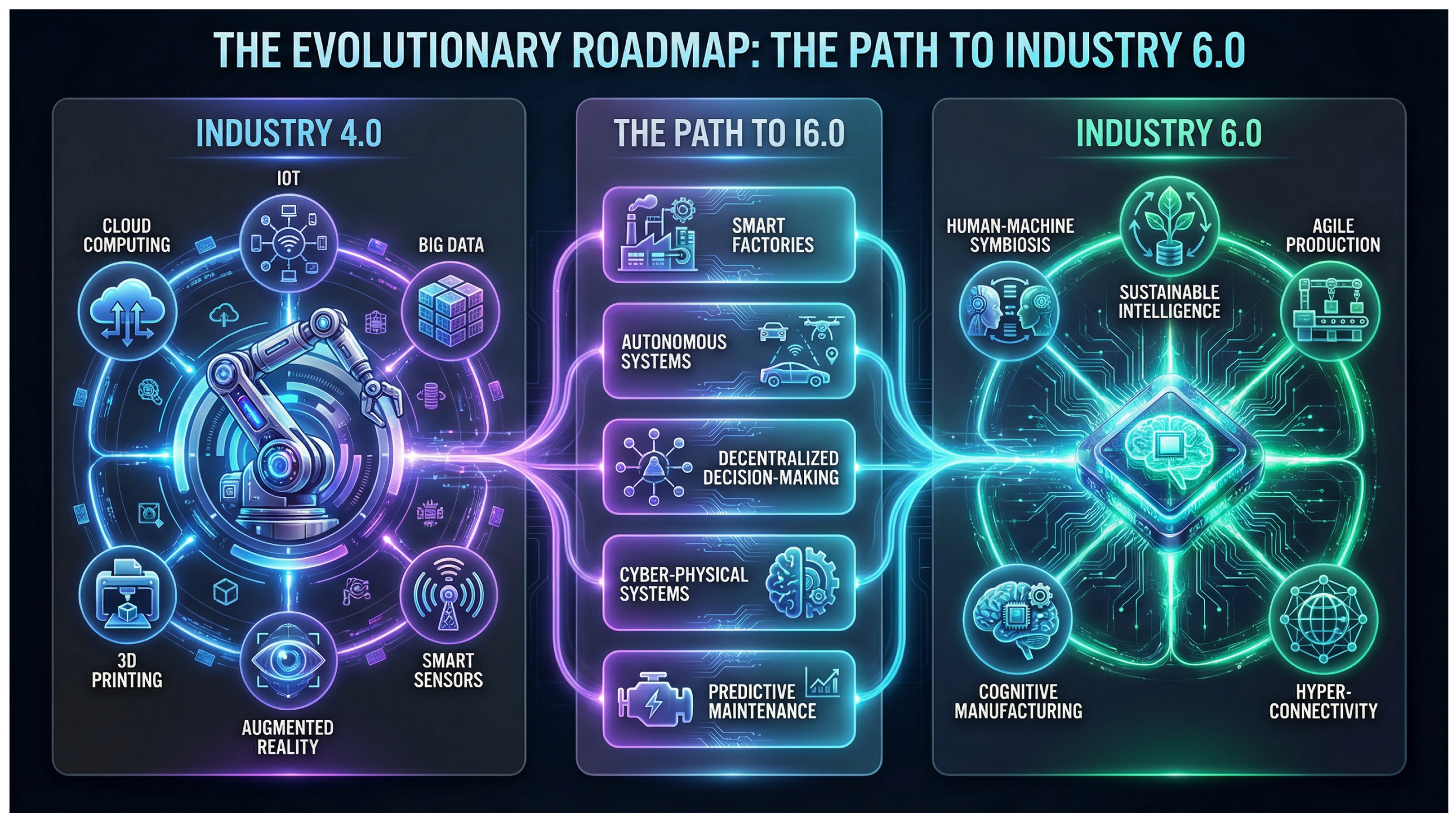
Some scholars argue that I5.0 is effectively a “corrective phase” for the social failings of I4.0. For environments that are already highly automated and sustainable by design [8], the transition is described as a “quantum leap” from I4.0 directly to the “cybernized services” of I6.0 [9]. Industry 6.0 is defined as “Ubiquitous, customer-driven, virtualized, and antifragile.” Because I6.0 relies on Artificial General Intelligence (AGI) and Quantum Computing, industries already pioneering these tools are essentially bypassing the “Collaborative/Cobot” focus of I5.0 [10]. While I4.0 focused on the “how” (technology), and I5.0 focused on the “why” (human-centricity/sustainability), I6.0 focuses on the “where next” (autonomous consciousness and circularity). If an organization already has a high-tech I4.0 base, they may view the “human-centric” social goals of I5.0 as a parallel policy track rather than a technical prerequisite, moving directly to the autonomous, self-healing networks of I6.0 [11]. Figure 3 illustrates the “Digital to Cybernized” leap.

2.3. I5.0: The Human-Centric and Resilient Correction

I5.0 evolved in the early 2020s as a reaction to the perceived deficiencies of the technology-centric I4.0 paradigm. It is characterized by an intensified emphasis on human-centricity, sustainability, and resilience. The European Commission has strongly advocated for this vision, asserting that I5.0 “prioritizes the well-being of the worker within the production process and employs new technologies to foster prosperity beyond mere employment and growth, all while honoring the planet’s production limits” [12].

Key characteristics of I5.0 [13] include:

• Human–Robot Collaboration: A shift from full automation [14] to a collaborative model where humans and robots (cobots) work together, leveraging the unique strengths of each.
• Personalization and Customization: A focus on meeting the individual needs of customers [15], moving away from mass production towards mass personalization.
• Sustainability and Resilience: A greater emphasis on resource efficiency [16], circular economy principles, and building resilient supply chains capable of withstanding global disruptions.

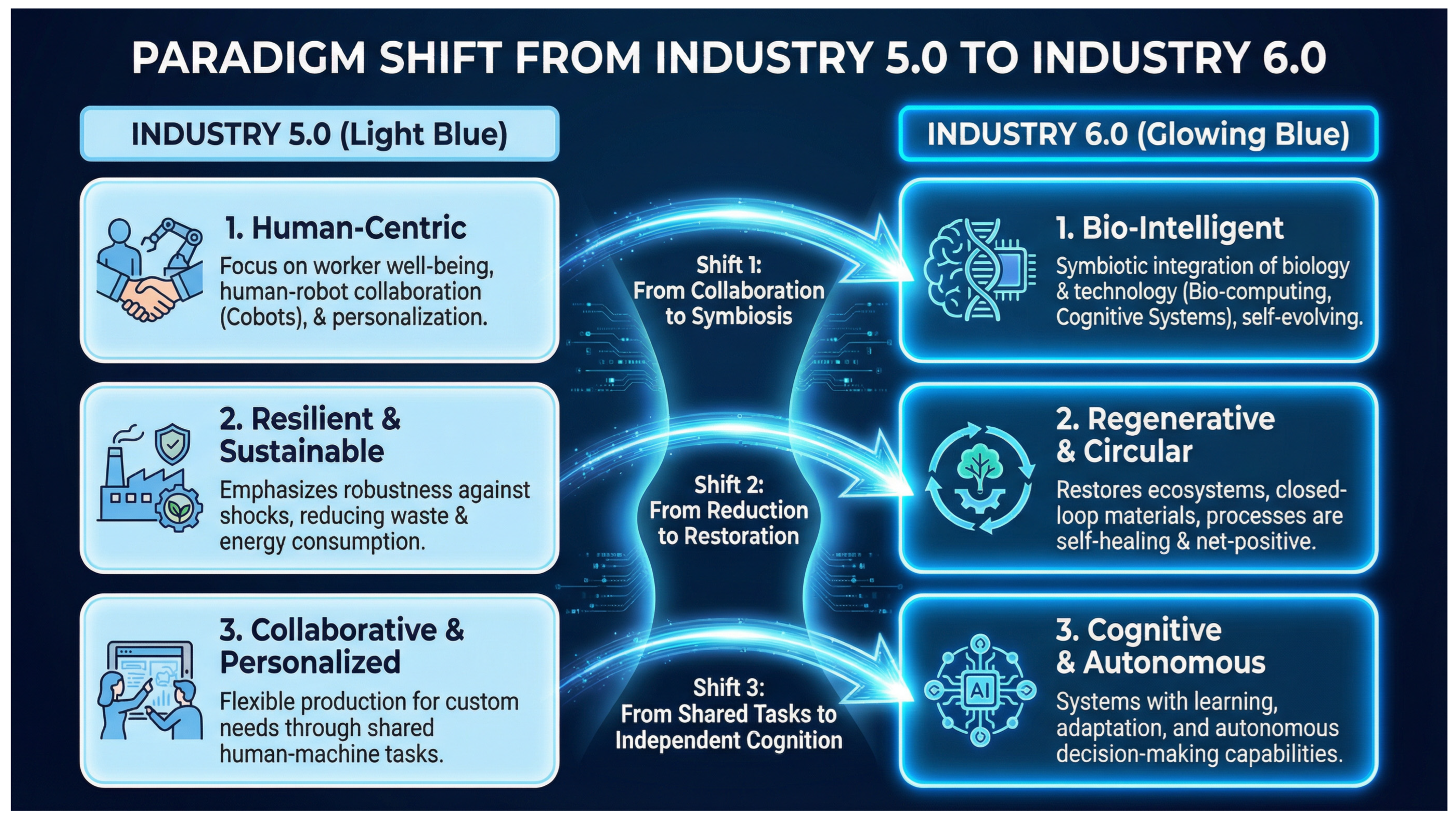
I5.0 can be seen as an attempt to temper the purely technological drive of I4.0 with a more holistic, humanistic, and socially responsible perspective [17]. It is a crucial bridge to I6.0 (see Figure 4), introducing the importance of sustainability and resilience that will become central tenets of the next paradigm.

2.4. I6.0: The Autonomous, Antifragile, and Regenerative Future

I6.0 signifies a conjectural yet progressively cohesive perspective on the future of manufacturing, expected to evolve in the 2030s and thereafter. It is not a singular, uniform concept, but a convergence of multiple significant tendencies documented in the literature [18]. I6.0 can be defined as a paradigm of autonomous, antifragile, and regenerative manufacturing [19], coordinated by GAI inside a hyper-connected, virtual–physical environment, synthesizing important ideas from foundational articles.

We can deconstruct this definition by examining the key paradigm shifts that distinguish I6.0 from its predecessors [1,11], as detailed in

Table 1. Key dimensions for each I4.0–I6.0.

Dimension	I4.0/I5.0 (Current)	I6.0 (Emerging)	Key References
Intelligence Model	Human-in-the-loop AI, assisting human decisions	Generative AI autonomy, co-creating and executing workflows	[1,6]
Operational Paradigm	Efficiency and robustness	Antifragility and adaptability	[9,20]
Sustainability Model	Standalone “green” initiatives, minimizing negative impact	Integrated circular economy, regenerative by design	[10,20]
System Boundary	The smart factory and its immediate supply chain	The hyper-connected virtual–physical ecosystem	[1,18]
Driving Technology	IoT, Cloud, Big Data, Cobots	Generative AI, Quantum Computing, 6G, IoX, Digital Twins	[1,10,20,21]
Human Role	Operator, collaborator, decision-maker	Strategic intent provider, ethicist, ecosystem designer	[21,22]

.

2.4.1. The Shift to Autonomy: Generative AI Orchestration

The most significant transformation in I6.0 is the transition from automation to autonomy, propelled by GAI. A fully automated production system can now be established in which a GAI interprets a natural language description of a product and independently coordinates a diverse array of robots to design, manufacture, and assemble it, entirely devoid of direct human intervention. This signifies a significant transformation in manufacturing, transitioning from a paradigm where people design and oversee processes to one where humans establish overarching objectives and AI systems manage the intricate details of implementation. A transition from “assist and advise” to “conceive and execute”. GAI has evolved from a mere analytical tool to a co-creator of value, proficient in producing innovative designs, optimizing intricate operations, and coordinating entire supply chains in real-time [23].

2.4.2. The Shift to Antifragility

The concept of antifragility is another cornerstone of I6.0 [24]. I5.0 underscores resilience, defined as the capacity to endure shocks, whereas I6.0 aspires to antifragility, characterized by the ability to thrive and benefit from shocks. In an era of heightened volatility, supply chain interruptions, and geopolitical instability, the capacity to learn and adapt from chaos constitutes a significant competitive advantage [25]. This necessitates a departure from the conventional Lean emphasis on eradicating all variation. Antifragile Lean systems would be structured to incorporate a degree of controlled chaos, utilizing it as a driver for learning and innovation. This entails constructing systems with strategic redundancy, modularity, and optionality, enabling them to reconfigure in response to evolving situations.

2.4.3. The Shift to Deep Sustainability: Circular and Regenerative Systems

I6.0 enhances the sustainability emphasis of I5.0, transitioning from a “do less harm” strategy to a “do more good” ideology. This entails the complete incorporation of circular economy and regenerative design ideas into the fundamental production process [26]. I6.0 characterizes manufacturing as a “catalyst for human flourishing, ecological regeneration, and adaptive intelligence.” Sustainability is now an integral design principle rather than a distinct Key Performance Indicator (KPI) to be weighed against cost and quality. The objective is to develop manufacturing systems that are not only zero-waste but also actively regenerative, aiding in the restoration of natural ecosystems [27,28].

2.4.4. The Shift to Hyper-Connected Ecosystems

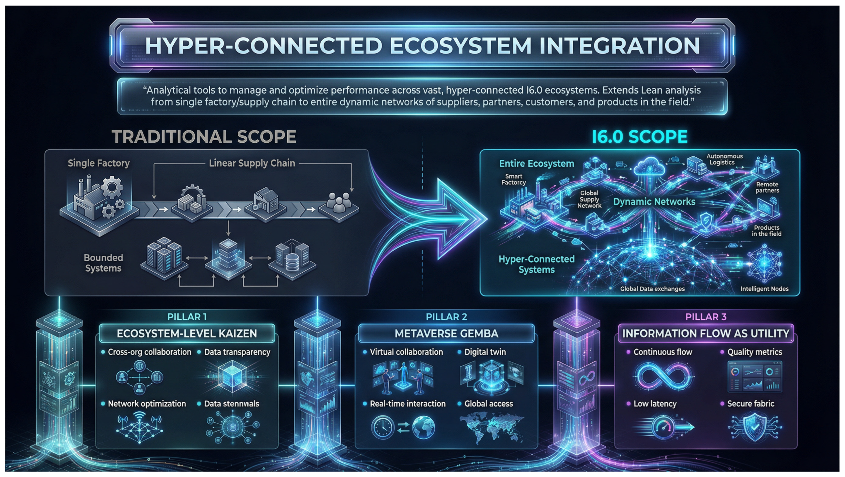
I6.0 extends the scope of the manufacturing system from the singular factory to the hyper-connected ecosystem. This is facilitated by technologies such as 6G networks, IoX, and metaverse-based digital twins. This concept entails the integration of the physical and digital realms into a cohesive, enduring virtual–physical reality [29].

A digital twin in I6.0 is not just a model of a machine; it is a live, interactive counterpart to the entire manufacturing ecosystem, from raw material suppliers to end customers. This “Metaverse Gemba” allows all stakeholders to interact with the system in real-time, enabling a level of collaborative optimization that is impossible today [30]. Figure 5 shows a structured conceptualization of I6.0.

In conclusion, the literature presents a clear and compelling vision of I6.0 as a paradigm of autonomous, antifragile, and regenerative manufacturing. This vision also reveals the profound limitations of current Lean analytical frameworks, which are the subject of the next section.

3. Research Gap Analysis: The Obsolescence of Current Lean Analytics

The significant paradigm shifts in I6.0, as detailed in the previous article, reveal essential deficiencies in the theoretical underpinnings of contemporary Lean manufacturing analytics. Frameworks developed for the comparatively stable, human-centered domains of I4.0/I5.0 are insufficient for the autonomous, unpredictable, and hyper-connected landscapes of the future. This part offers a comprehensive study of these deficiencies, illustrating the pressing necessity for a novel theoretical framework.

3.1. The Inadequacy of “Robustness” in an Antifragile World

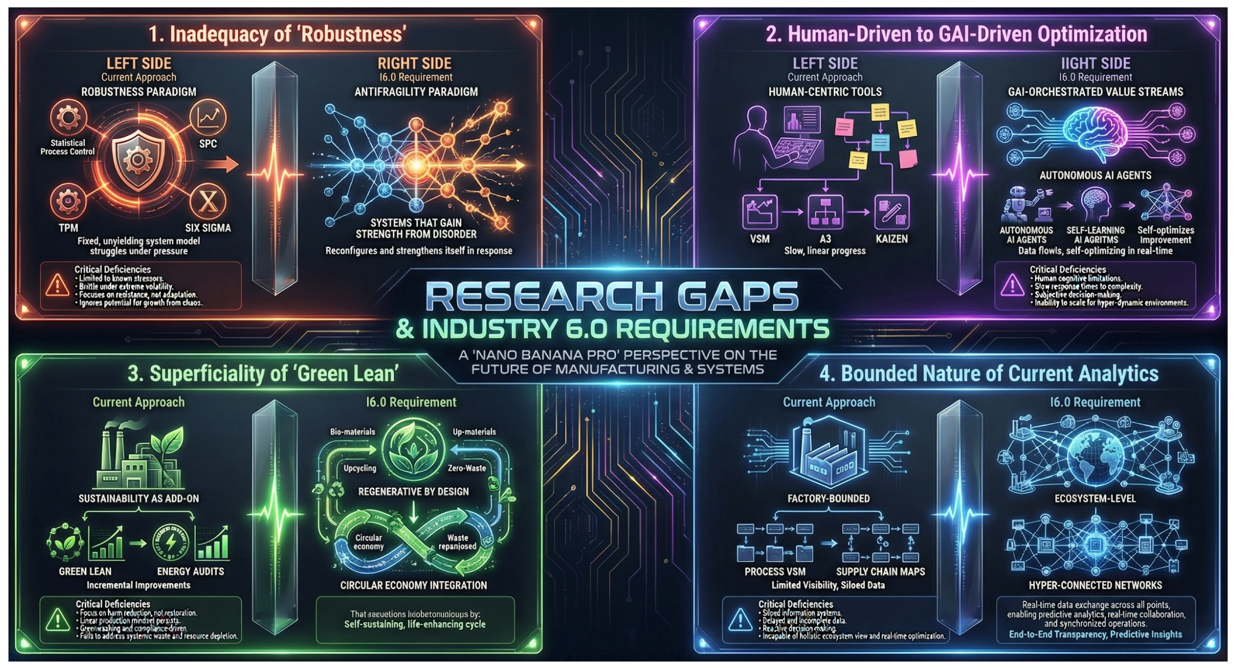
Conventional Lean analytics, as well as contemporary quality control, is based on the notion of robustness. A process is deemed robust if its performance remains unaffected by sources of variance. The fundamental principle of Statistical Process Control (SPC) is to recognize and eradicate “special cause” variance to establish a stable and predictable process. Total Productive Maintenance (TPM) seeks to eradicate the “six big losses” to avert equipment-related interruptions [31]. This emphasis on stability, although useful in controlled settings, becomes a disadvantage in a world marked by heightened Volatility, Uncertainty, Complexity, and Ambiguity (VUCA) [32].

I6.0 demands antifragility. Antifragility benefits from shocks; it thrives and grows when exposed to VUCA [33]. Existing Lean metrics fail to assess antifragility. In fact, they quantify its antithesis: the lack of variation. No recognized analytical framework exists within Lean for the design or optimization of systems that get strength from disorder. This represents a critical theoretical deficiency that highlights an inadequacy in the language, the metrics, and the models to transition from a defensive stance of robustness to a proactive approach of antifragility.

3.2. The Shift from Human-Driven to GAI-Driven Optimization

Current Lean analytics are fundamentally human-centric. Core Lean tools are predicated on human observation, analysis, and decision-making:

• Value Stream Mapping (VSM): A team of people walks the Gemba, observes the process, and manually draws a map [34].
• A3 Problem Solving: A structured, collaborative problem-solving process guided by a human mentor [35].
• Kaizen Events: A focused, week-long event where a cross-functional team works to improve a specific process [36].

In “Digital Lean,” AI is primarily employed as an analytical instrument to aid human managers in enhancing decision-making. I6.0 will be defined by Generative AI-Orchestrated Value Streams, wherein autonomous AI agents execute real-time choices and manage intricate workflows throughout vast ecosystems [37].

This creates a significant theoretical void. Existing Lean frameworks have no basis for analyzing, managing, or optimizing these emergent, AI-driven systems. There is a need for metrics to evaluate the performance of a GAI orchestrator. How do we apply the principle of “Respect for People” when the “person” making the decision is an AI? How do we conduct a “Gemba walk” in a process that exists only as a set of dynamic interactions between decentralized AI agents? Current Lean theory provides no answers.

3.3. The Superficiality of “Green Lean”

The incorporation of sustainability into Lean methodologies, referred to as “Green Lean,” is an expanding and significant area of study [38]; nonetheless, it frequently regards environmental objectives as distinct, supplementary factors. The emphasis is generally on specific initiatives such as energy conservation, waste reduction, or the utilization of sustainable materials. These objectives are commendable; yet, they inadequately address the profound, systemic incorporation of circular and regenerative ideas required by I6.0.

I6.0 envisions a paradigm in which the manufacturing process is not merely “less harmful” to the environment, but is actively regenerative, aiding in the restoration of natural capital. It necessitates a transition from a linear “take-make-dispose” paradigm to a comprehensive circular model, wherein items are engineered for disassembly, remanufacturing, and reuse from inception. Contemporary Lean analytics are deficient in real-time, multi-dimensional models essential for prioritizing circularity and regeneration alongside cost and quality as primary objectives [39]. Questions such as “What is the real-time circularity score of this production line?” or “How does this process change contribute to the regeneration of the local watershed?” cannot be answered.

3.4. The Bounded Nature of Current Analytics

Traditional Lean analytics are intrinsically limited. The unit of analysis is generally a singular process, an individual factory, or, at most, a linear supply chain. This reflects Lean’s roots in the TPS, which aimed to enhance the efficiency of a singular, vertically integrated enterprise [40]. I6.0 functions inside a hyper-connected ecosystem of virtual and physical assets, facilitating smooth data flow among businesses, customers, and products in the field. This engenders a degree of complexity and interrelation that conventional analytical instruments are incapable of managing.

There is no widely adopted, standardized, real-time “ecosystem-level Lean analytics” architecture that is consistently integrated with continuous data streams and cyber–physical representations [41] (as opposed to periodic, project-based mapping and improvement cycles) [42]. How does the manufacturing enterprise identify and eliminate “ecosystem wastes” like information asymmetry between partners, data friction at system interfaces, or misaligned incentives in a decentralized network? How do they create a VSM for a process that spans a dozen different companies and is constantly reconfiguring itself?

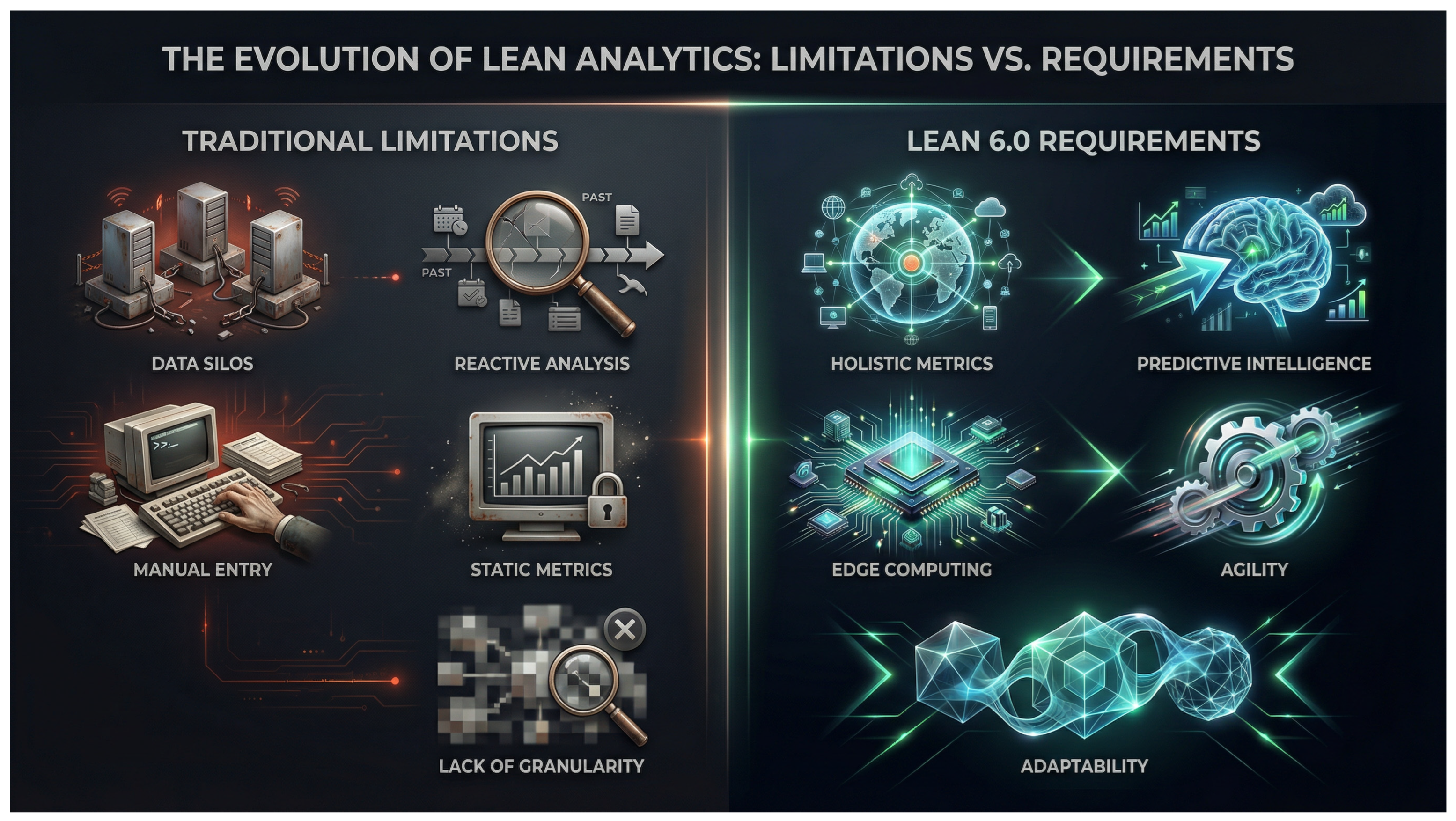
These four gaps (see Figure 6) are not minor shortcomings; they represent a fundamental disconnect between the theoretical foundations of current Lean analytics and the emerging reality of I6.0. A new theoretical framework is urgently needed to bridge this chasm.

4. Mathematical Modeling of the I6LA Framework

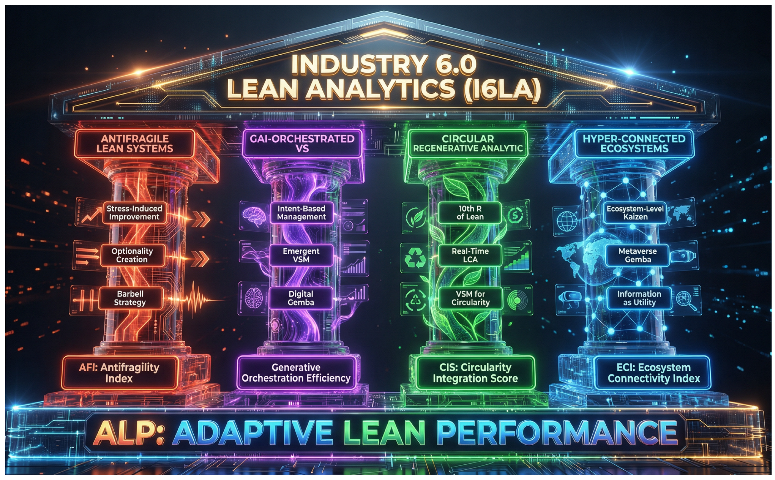
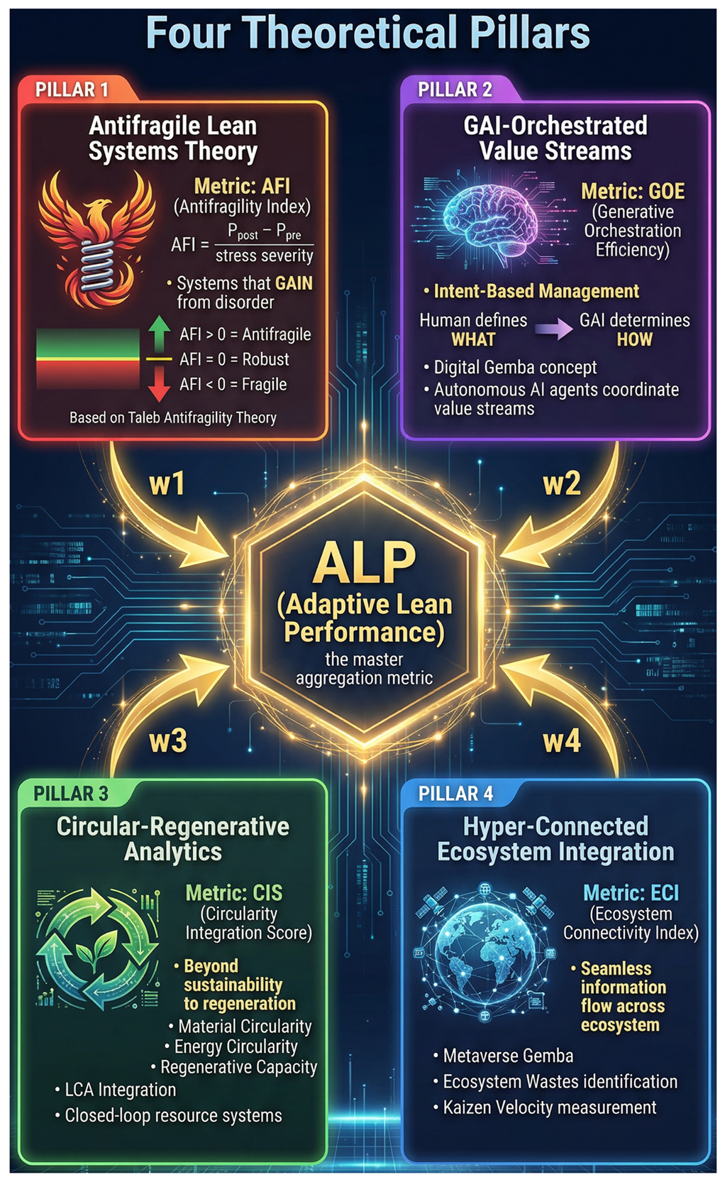
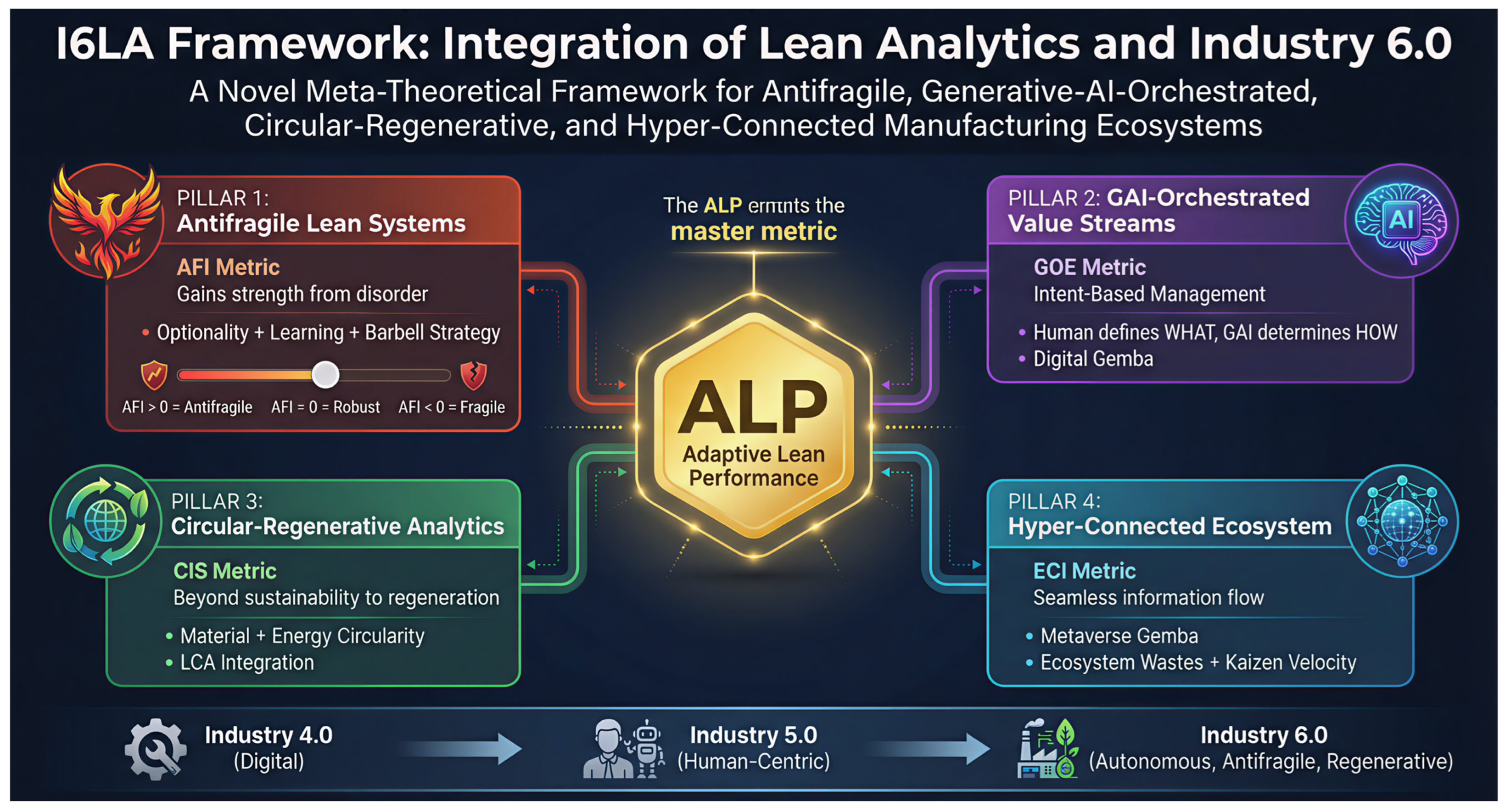
To address the critical research gaps identified above, the I6LA framework is proposed. The I6LA framework is a meta-theoretical construct intended to establish the analytical foundations for Lean manufacturing in the context of I6.0. It consists of four interrelated theoretical pillars (see Figure 7), each targeting a fundamental shortcoming in existing Lean analytics.

4.1. Pillar 1: Antifragile Lean Systems Theory

Definition: This pillar redefines the core Lean objective from creating stable, robust processes to designing antifragile systems that gain capability and performance when exposed to stressors, volatility, and uncertainty. It integrates antifragility into the Lean philosophy, arguing that in the unpredictable environments of I6.0, the ability to profit from disorder is a greater competitive advantage than the ability to resist it.

Theoretical Grounding: The concept of antifragility distinguishes it from resilience (the ability to withstand shocks) and robustness (the ability to remain unchanged by shocks) [43]. An antifragile system, by contrast, improves as a result of shocks. This pillar connects antifragility abstract theory to the concrete practices of manufacturing, proposing a new set of design principles and performance metrics [44,45].

Key Principles:

• From Waste Elimination to Optionality Creation: Traditional Lean focuses on eliminating the seven wastes (muda) to create a streamlined, efficient process. Antifragile Lean complements this by prioritizing the creation of optionality. This means building systems with strategic redundancy, modular product and process architectures, and multiple sourcing strategies. While these might appear as “waste” from a traditional Lean perspective (e.g., excess inventory, underutilized capacity), they are re-framed as valuable options that allow the system to adapt and thrive in the face of unexpected events. The analytical challenge is to distinguish between “bad” waste and “good” optionality.
• Stress-Induced Continuous Improvement: The Lean principle of Kaizen (continuous improvement) is re-imagined. Instead of relying solely on planned improvement events, Antifragile Lean treats disruptions (e.g., supply chain delays, demand spikes, equipment failures) as opportunities for learning and adaptation. The framework includes mechanisms for “stress testing” the system with controlled disruptions and using the resulting data to drive system evolution. This is a more dynamic and event-driven form of continuous improvement.
• Barbell Asymmetry in Risk and Innovation Management Strategy in Manufacturing: This principle provides a practical approach to managing risk and innovation. It involves allocating the majority of resources (e.g., 90%) to highly reliable, efficient, and low-risk processes (the “safe” bar). The remaining resources (e.g., 10%) are invested in high-risk, high-reward experimental processes, such as testing novel materials or radical new production methods (the “speculative” bar). This strategy allows the system to benefit from massive upside potential from innovation while being protected from catastrophic failure (risk).

4.1.1. Antifragility Index (AFI)

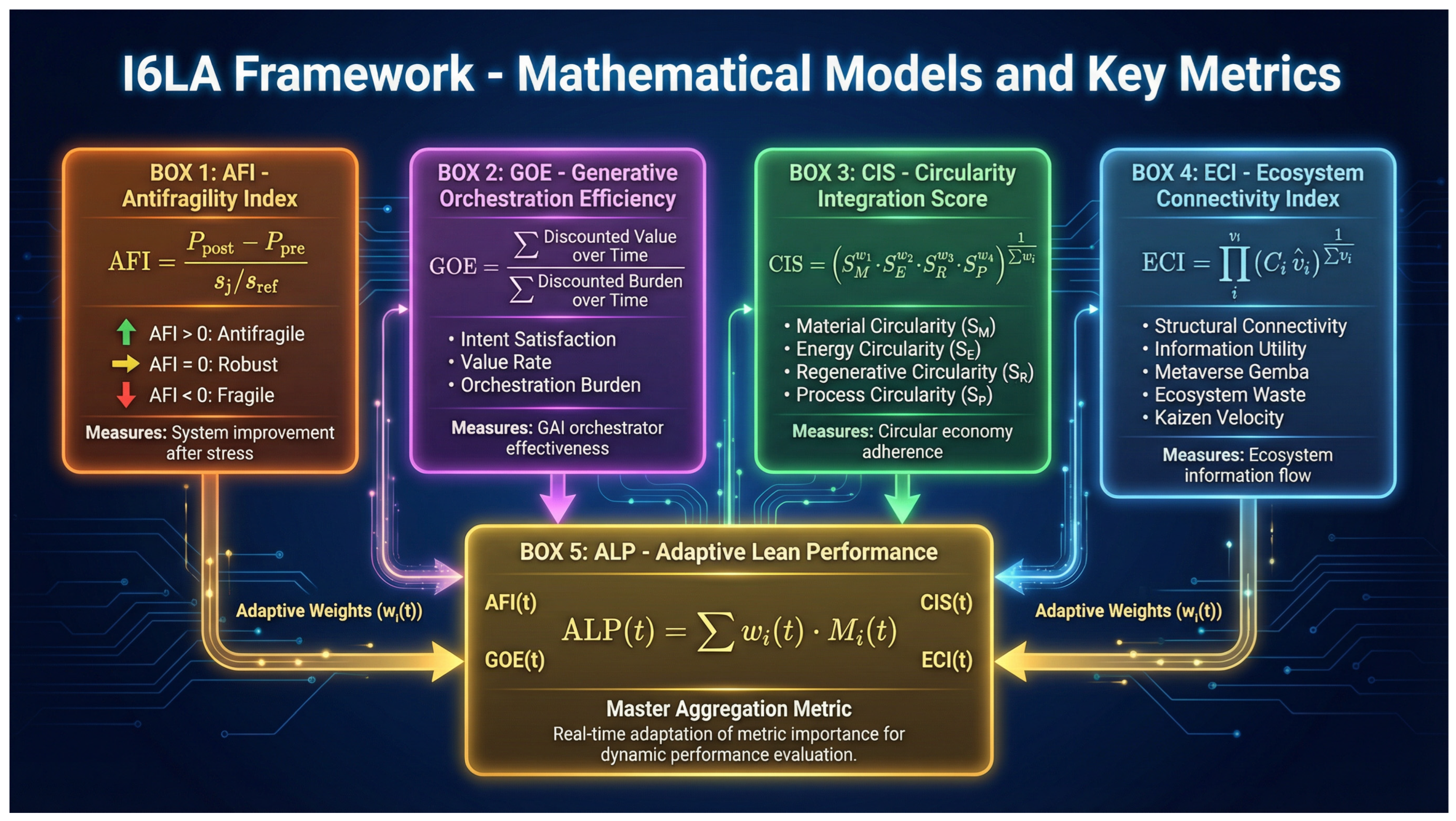
The pillar asserts that antifragility in Lean manufacturing is not merely “performance after a shock,” but a measurable capability that emerges from three design mechanisms: optionality creation, stress-induced learning, and barbell risk–innovation asymmetry. Consequently, the index must quantify antifragility as a stress-response derivative of performance while explicitly conditioning that derivative on those three mechanisms. The most direct way to do this is to define antifragility as an estimated marginal performance gain per unit stress, decomposed into mechanism-consistent components through interaction structure. This produces one scalar index that is antifragile if and only if the system’s expected performance response to stress is positive after accounting for optionality, learning, and barbell structure (see

Table A1. AFI symbols and units (Pillar 1).

Symbol	Meaning	Units
j	Disruption (or injected test) event index, j = 1,…,N	dimensionless (index)
N	Number of events in the evaluation set	count
tj(start)	Start time of event j	time (same unit as timestamps)
tj(end)	End time of event j	time (same unit as timestamps)
P(t)	Chosen Lean performance signal over time (e.g., OEE, FTT, throughput)	depends on signal; typically a dimensionless ratio or rate
Tpre	Length of pre-event averaging window	time
Tpost	Length of post-event averaging window	time
Tlag	Adaptation lag between the event end and the post-window start	time
Pj(pre)	Time-average of P(t) over the pre-event window for event j	same as P(t)
Pj(post)	Time-average of P(t) over the post-event window for event j	same as P(t)
rj	Event performance response log-ratio ln(Pj(post)/Pj(pre))	dimensionless
sj(raw)	Raw disruption severity for event j (natural units for the event type)	event-type dependent (e.g., %, days, hours)
sref(τj)	Positive reference severity scale for event type τj	same as sj(raw)
Sj	Normalized severity Sj = sj(raw)/sref(τj)	dimensionless
O(t)	Optionality stock state variable	dimensionless index
Oj(pre)	Pre-event average optionality for event j	dimensionless
Oj(post)	Post-event average optionality for event j	dimensionless
ΔOj	Optionality creation during/after event j: Oj(post) − Oj(pre)	dimensionless
C(t)	Effective available capacity (planning granularity)	units of capacity (e.g., units/time or tool-hours)
Q(t)	Required capacity (same granularity as C(t))	same as C(t)
ρt	Redundancy ratio ρt = C(t)/Q(t) (bounded as defined)	dimensionless
ρmax	Cap on redundancy ratio treated as “strategic”	dimensionless
R(t)	Redundancy subscore derived from ρt and ρmax	dimensionless (0–1)
κ(t)	Coupling proxy used to quantify modularity	depends on proxy; treated as dimensionless after normalization
κref	Reference coupling level for κ(t)	same as κ(t)
Mmod(t)	Modularity subscore (denoted M(t) in AFI pillar text)	dimensionless (0–1)
pk(t)	Share of source k for a critical component (multi-sourcing shares)	dimensionless (fractions sum to 1)
K	Number of qualified sources used in diversity calculation	count
Ds(t)	Multi-sourcing diversity subscore (concentration-based)	dimensionless (0–1)
wR, wM, wD	Weights for redundancy, modularity, and diversity in optionality	dimensionless (sum to 1)
Tj(rec)	Recovery time for event j (first time P(t) recovers above threshold)	time
θ	Recovery threshold multiplier relative to pre-event performance	dimensionless
Lj	Learning-from-stress signal from recovery time change vs prior comparable event	dimensionless
ℓ	Downside loss random variable for barbell risk	loss units (e.g., cost, days, throughput loss)
q	Tail probability level used for VaR/CVaR	dimensionless (probability)
VaRφ(ℓ)	Value-at-risk of loss ℓ at level q	same as ℓ
CVaRφ(ℓ)	Conditional value-at-risk of loss ℓ at level q	same as ℓ
m	Experiment index in speculative bar, m = 1,…,M	dimensionless (index)
M	Number of speculative experiments (context-dependent; not the ALP metric vector)	count
rm(exp)	Log return (or return proxy) of experiment m	dimensionless (log-return) or return units as defined
U	Mean realized speculative upside across experiments	same as rm(exp)
α	Safe-bar resource fraction in barbell strategy	dimensionless (fraction)
ε	Small numerical constant to avoid division by zero/log(0)	dimensionless
B	Barbell asymmetry variable (upside relative to extreme downside exposure)	dimensionless
β0,…,β5	Regression coefficients in event-level gain-per-stress model	units depend on regressor scaling; AFI itself is dimensionless
εj	Regression error term for event j	same as dependent variable rj/Sj (dimensionless)
xj, X, y, β	Regression covariate vector, design matrix, response vector, coefficient vector	dimensionless after normalization
S, Opre, ΔO, L	Sample means of Sj, Oj(pre), ΔOj, Lj used in AFI definition	dimensionless
AFI	Antifragility Index (fitted expected gain-per-stress under typical conditions)	dimensionless
i	Disruption instance index within type k (severity normalization)	dimensionless (index)
k	Disruption type index (taxonomy class)	dimensionless (index)
sik	Realized severity, for instance, i of type k	same axis as AFI stress term (e.g., normalized downtime)
srefk	Reference severity scale for type k (robust central tendency with uncertainty)	same as sik

in Appendix A for all related mathematical symbols).

Let disruptive (or intentionally injected) events be indexed by $j=1,\dots ,N$. Each event $j$ has a start time $t_j^{\mathrm{s}\mathrm{t}\mathrm{a}\mathrm{r}\mathrm{t}}$, an end time $t_j^{\mathrm{e}\mathrm{n}\mathrm{d}}$, and a strictly positive normalized severity $S_j>0$. Let $P(t)>0$ be a chosen Lean performance signal (for example, OEE, FTT, throughput, or a composite), measured over time. Fix three analyst-defined constants: a pre-window length $T_{\mathrm{p}\mathrm{r}\mathrm{e}}>0$, a post-window length $T_{\mathrm{p}\mathrm{o}\mathrm{s}\mathrm{t}}>0$, and an adaptation lag $T_{\mathrm{l}\mathrm{a}\mathrm{g}}\ge 0$. Define the pre- and post-event performance levels by time averages:

$$P_j^{\mathrm{p}\mathrm{r}\mathrm{e}}={\displaystyle \frac{1}{T_{\mathrm{p}\mathrm{r}\mathrm{e}}}}{\int }_{t_j^{\mathrm{s}\mathrm{t}\mathrm{a}\mathrm{r}\mathrm{t}}-T_{\mathrm{p}\mathrm{r}\mathrm{e}}}^{t_j^{\mathrm{s}\mathrm{t}\mathrm{a}\mathrm{r}\mathrm{t}}}P(t) dt,P_j^{\mathrm{p}\mathrm{o}\mathrm{s}\mathrm{t}}={\displaystyle \frac{1}{T_{\mathrm{p}\mathrm{o}\mathrm{s}\mathrm{t}}}}{\int }_{t_j^{\mathrm{e}\mathrm{n}\mathrm{d}}+T_{\mathrm{l}\mathrm{a}\mathrm{g}}}^{t_j^{\mathrm{e}\mathrm{n}\mathrm{d}}+T_{\mathrm{l}\mathrm{a}\mathrm{g}}+T_{\mathrm{p}\mathrm{o}\mathrm{s}\mathrm{t}}}P\left(t\right) dt.$$

(1)

Define the event performance response as a log-ratio (dimensionless):

$$r_j=\ln \left({\displaystyle \frac{P_j^{\mathrm{p}\mathrm{o}\mathrm{s}\mathrm{t}}}{P_j^{\mathrm{p}\mathrm{r}\mathrm{e}}}}\right).$$

(2)

This choice ensures comparability across plants and metrics because $r_j$ represents proportional change. Severity normalization is defined as follows. For each event type ${\tau }_j$ (demand shock, supply disruption, equipment failure, etc.), compute a raw severity $s_j^{\mathrm{r}\mathrm{a}\mathrm{w}}>0$ in its natural units (percent change, days, hours). Choose a positive reference scale $s_{\tau }^{\mathrm{r}\mathrm{e}\mathrm{f}}>0$ for each type $\tau$ (typically the historical median raw severity for that type). Then, set

$$S_j={\displaystyle \frac{s_j^{\mathrm{r}\mathrm{a}\mathrm{w}}}{s_{{\tau }_j}^{\mathrm{r}\mathrm{e}\mathrm{f}}}},$$

(3)

so $S_j$ is dimensionless and interpretable as “multiples of typical severity.” Severity is a context-dependent variable:

• Demand shock: $s_j^{\mathrm{r}\mathrm{a}\mathrm{w}}=\mid \Delta \% \mathrm{orders}\mid$;

• Supply disruption: $s_j^{\mathrm{r}\mathrm{a}\mathrm{w}}=\mathrm{outage} \mathrm{duration} (\mathrm{days})$;

• Equipment failure: $s_j^{\mathrm{r}\mathrm{a}\mathrm{w}}=\mathrm{MTTR} (\mathrm{hours})$.

The optionality mechanism must be captured as a measurable state variable $O(t)\in [0,1]$ representing “good optionality” rather than undirected waste.

Let $C(t)$ be effective, available capacity, and $D(t)$ required capacity over the same planning granularity, with $D(t)>0$. Define a redundancy ratio $\rho (t)=(C(t)-D(t))/D(t)$. Choose a cap ${\rho }_{\mathrm{m}\mathrm{a}\mathrm{x}}>0$ that represents the largest redundancy considered “strategic” rather than indiscriminate. Therefore, redundancy can be expressed as

$$R\left(t\right)=\min \left\{1,\max \left\{0,{\displaystyle \frac{\rho \left(t\right)}{{\rho }_{\mathrm{m}\mathrm{a}\mathrm{x}}}}\right\}\right\}.$$

(4)

Let $\kappa (t)\ge 0$ be a coupling proxy (for example, average routing coupling score, interface count normalized to a baseline, or changeover coupling index). Choose ${\kappa }_{\mathrm{r}\mathrm{e}\mathrm{f}}>0$ as a reference coupling level. Therefore, modularity can be expressed as

$$M\left(t\right)={\displaystyle \frac{1}{1+\frac{\kappa \left(t\right)}{{\kappa }_{\mathrm{r}\mathrm{e}\mathrm{f}}}}}.$$

(5)

Suppose a critical component is supplied by $K$ qualified sources with shares $p_k(t)\ge 0$ and ${\sum }_{k=1}^K{p}_k(t)=1$. Therefore, multi-sourcing diversity can be expressed as

$$D_s(t)=1-\sum _{k=1}^K{p}_k(t{)}^2.$$

(6)

which increases as sourcing becomes less concentrated.

Choose weights $w_R,w_M,w_D\ge 0$ with $w_R+w_M+w_D=1$. And the optionality stock can be defined as

$$O(t)=w_{R}R(t)+w_{M}M(t)+w_D{D}_s\left(t\right).$$

(7)

Therefore, event-level pre-optionality and optionality change can be defined as

$$O_j^{\mathrm{p}\mathrm{r}\mathrm{e}}={\displaystyle \frac{1}{T_{\mathrm{p}\mathrm{r}\mathrm{e}}}}{\int }_{t_j^{\mathrm{s}\mathrm{t}\mathrm{a}\mathrm{r}\mathrm{t}}-T_{\mathrm{p}\mathrm{r}\mathrm{e}}}^{t_j^{\mathrm{s}\mathrm{t}\mathrm{a}\mathrm{r}\mathrm{t}}}O(t) dt,\Delta O_j=O_j^{\mathrm{p}\mathrm{o}\mathrm{s}\mathrm{t}}-O_j^{\mathrm{p}\mathrm{r}\mathrm{e}},$$

(8)

where

$$O_j^{\mathrm{p}\mathrm{o}\mathrm{s}\mathrm{t}}={\displaystyle \frac{1}{T_{\mathrm{p}\mathrm{o}\mathrm{s}\mathrm{t}}}}{\int }_{t_j^{\mathrm{e}\mathrm{n}\mathrm{d}}+T_{\mathrm{l}\mathrm{a}\mathrm{g}}}^{t_j^{\mathrm{e}\mathrm{n}\mathrm{d}}+T_{\mathrm{l}\mathrm{a}\mathrm{g}}+T_{\mathrm{p}\mathrm{o}\mathrm{s}\mathrm{t}}}O(t) dt.$$

(9)

The stress-induced continuous improvement mechanism must be represented as a learning variable that increases when the system converts disruptions into faster restoration and better future handling. Let $\left.\theta \in (0,1\right]$ be a recovery threshold. Thus, recovery time can be defined as

$$T_j^{\mathrm{r}\mathrm{e}\mathrm{c}}=\mathrm{i}\mathrm{n}\mathrm{f}\left\{t-t_j^{\mathrm{e}\mathrm{n}\mathrm{d}}: P(t)\ge \theta P_j^{\mathrm{p}\mathrm{r}\mathrm{e}}\right\}.$$

(10)

A dimensionless learning-from-stress signal is defined using the prior comparable event within the same event type ${\tau }_j$. Let $j^{-}$ denote the most recent event before $j$ with ${\tau }_{j^{-}}={\tau }_j$ (if none exists, the learning term for $j$ is defined as $0$). Then,

$$L_j=\left\{\begin{array}{cc}\ln \left(\frac{T_{j^{-}}^{\mathrm{rec}}}{T_j^{\mathrm{rec}}}\right);& \mathrm{if} \mathrm{a} \mathrm{prior} \mathrm{same-type} \mathrm{event} \mathrm{exists},\\ 0,& \mathrm{otherwise}.\end{array}\right.$$

(11)

With this definition, $L_j>0$ means recovery became faster relative to the previous comparable disruption, which is precisely “stress-induced Kaizen.”

The risk and innovation mechanism must measure asymmetric payoff: controlled downside in the safe bar and upside capture in the speculative bar. Let $\alpha \in (0,1)$ be the fraction of resources devoted to the safe bar. Define a downside loss per event as ${\mathcal{l}}_j=\mathrm{m}\mathrm{a}\mathrm{x}\{0,-r_j\}$. Choose a tail probability $q\in (0,1)$. Therefore, value-at-risk can be expressed as:

$${\mathrm{V}\mathrm{a}\mathrm{R}}_q\left(\mathcal{l}\right)=\inf \left\{x:\mathrm{Pr}\left(\mathcal{l}\le x\right)\ge q\right\}$$

(12)

and conditional value-at-risk as

$${\mathrm{C}\mathrm{V}\mathrm{a}\mathrm{R}}_q\left(\mathcal{l}\right)=\mathbb{E} \left[\mathcal{l}\mid \mathcal{l}\ge {\mathrm{V}\mathrm{a}\mathrm{R}}_q\left(\mathcal{l}\right)\right]$$

(13)

The speculative upside is defined as follows. Over the same evaluation horizon, let experiments be indexed $m=1,\dots ,M$, each with a log return $r_m^{\mathrm{e}\mathrm{x}\mathrm{p}}=\mathrm{l}\mathrm{n}(P_m^{\mathrm{e}\mathrm{x}\mathrm{p},\mathrm{p}\mathrm{o}\mathrm{s}\mathrm{t}}/P_m^{\mathrm{e}\mathrm{x}\mathrm{p},\mathrm{p}\mathrm{r}\mathrm{e}})$. Then, the mean realized upside is

$$U={\displaystyle \frac{1}{M}}\sum _{m=1}^M\mathrm{m}\mathrm{a}\mathrm{x}\{0,r_m^{\mathrm{e}\mathrm{x}\mathrm{p}}\}.$$

(14)

A small constant $\epsilon >0$ (e.g., ${10}^{-6}$) is chosen to prevent division by zero. Thus, the Barbell asymmetric variable B is

$$B=\ln \left(1+{\displaystyle \frac{\left(1-\alpha \right) U}{\alpha {\mathrm{C}\mathrm{V}\mathrm{a}\mathrm{R}}_q\left(\mathcal{l}\right)+\epsilon }}\right).$$

(15)

This is dimensionless and increases when upside is captured relative to extreme downside exposure. Antifragility must be a property of how performance responds to stress, not merely an average after-stress difference. Therefore, an event-level regression can be defined as

$${\displaystyle \frac{r_j}{S_j}}={\beta }_0+{\beta }_1{S}_j+{\beta }_2{O}_j^{\mathrm{p}\mathrm{r}\mathrm{e}}+{\beta }_3\Delta O_j+{\beta }_4{L}_j+{\beta }_{5}B+{\epsilon }_j,j=1,\dots ,N.$$

(16)

The left-hand side is the realized gain per unit stress, and the right-hand side decomposes that gain into (i) a baseline term, (ii) a nonlinearity-in-stress term, and (iii) the three pillar mechanisms, with optionality appearing both as a pre-existing capacity to adapt ($O_j^{\mathrm{p}\mathrm{r}\mathrm{e}}$) and as optionality creation ($\Delta O_j$). Let

$$y_j={\displaystyle \frac{r_j}{S_j}},x_j=\left[\begin{array}{c}1\\ S_j\\ O_j^{\mathrm{p}\mathrm{r}\mathrm{e}}\\ \Delta O_j\\ L_j\\ B\end{array}\right],X=\left[\begin{array}{c}{x}_1^{\mathrm{\top }}\\ x_2^{\mathrm{\top }}\\ ⋮\\ x_N^{\mathrm{\top }}\end{array}\right],\mathrm{y}=\left[\begin{array}{c}{y}_1\\ y_2\\ ⋮\\ y_N\end{array}\right].$$

(17)

The ordinary least squares estimator is

$$\widehat{\beta }=(X^{\mathrm{\top }}X{)}^{-1}{X}^{\mathrm{\top }}\mathrm{y},$$

(18)

where $\widehat{\beta }=[{\widehat{\beta }}_0,{\widehat{\beta }}_1,{\widehat{\beta }}_2,{\widehat{\beta }}_3,{\widehat{\beta }}_4,{\widehat{\beta }}_5{]}^{\mathrm{\top }}$, provided $X^{\mathrm{\top }}X$ is invertible. If $X^{\mathrm{\top }}X$ is not invertible due to collinearity, then the redundant covariate can be removed or ridge regularization can be applied; the ridge estimator is ${\widehat{\beta }}_{\lambda }=(X^{\mathrm{\top }}X+\lambda I{)}^{-1}{X}^{\mathrm{\top }}\mathrm{y}$ with $\lambda >0$. The pillar definition of antifragility is “improves because of stress,” operationalized as the system’s expected gain-per-stress after accounting for optionality, learning, and Barbell asymmetry. That object is the fitted conditional mean of $y_j$, averaged over observed conditions. Therefore, the sample means are defined as

$$\overline{S}={\displaystyle \frac{1}{N}}\sum _{j=1}^N{S}_j,{\overline{O}}^{\mathrm{p}\mathrm{r}\mathrm{e}}={\displaystyle \frac{1}{N}}\sum _{j=1}^N{O}_j^{\mathrm{p}\mathrm{r}\mathrm{e}},\Delta \overline{O}={\displaystyle \frac{1}{N}}\sum _{j=1}^N\Delta O_j,\overline{L}={\displaystyle \frac{1}{N}}\sum _{j=1}^N{L}_j.$$

(19)

Then AFI is defined as

$$\mathrm{A}\mathrm{F}\mathrm{I}={\widehat{\beta }}_0+{\widehat{\beta }}_1\overline{S}+{\widehat{\beta }}_2{\overline{O}}^{\mathrm{p}\mathrm{r}\mathrm{e}}+{\widehat{\beta }}_3\Delta \overline{O}+{\widehat{\beta }}_4\overline{L}+{\widehat{\beta }}_{5}B,$$

(20)

with the interpretation that $\mathrm{A}\mathrm{F}\mathrm{I}$ is the estimated expected value of $r/S$ under typical observed conditions, explicitly decomposed into the three pillar mechanisms.

Interpretation:

• AFI > 0: The system is antifragile. It improved as a result of the stressor.
• AFI = 0: The system is robust. It was unaffected by the stressor.
• AFI < 0: The system is fragile. Its performance degraded as a result of the stressor.

4.1.2. AFI Severity Normalization

The Antifragility Index in Section 4.1.1 normalizes realized disruption severity using a positive reference scale $s_j^{ref}$ to ensure comparability of gain-per-stress across heterogeneous disruption types. For disruption types that are novel, unprecedented, or insufficiently observed, a historical median severity may be unavailable or statistically unstable. In such cases, $s_j^{ref}$ is defined operationally as a governed baseline estimator with explicit uncertainty, rather than as a fixed empirical constant. The baseline is initialized using a principled construction rule and is subsequently updated as evidence accumulates, ensuring that severity normalization remains well-defined and does not depend on ad hoc assumptions. For each disruption instance $e$ of type $j$, the framework defines a nonnegative realized severity $s_{e,j}$ on the same operational axis used by the AFI stress term (e.g., normalized downtime, throughput loss, OEE drawdown, service shortfall, or a composite operational impairment score). The reference scale $s_j^{ref}$ is then defined as a robust central tendency functional of the severity distribution for type $j$, denoted $Q_{0.50}(S_j)$, with an explicit uncertainty interval $\left[Q_{0.05}(S_j),Q_{0.95}(S_j)\right]$. This construction directly supports rare-event settings where sample sizes are small and tail risk is material; it also permits principled updating as evidence accumulates. Bayesian updating frameworks for rare events provide a coherent basis for this approach when empirical observations are limited and must be combined with structured priors [46].

Baseline Construction When Historical Medians Are Unavailable

When type $j$ has insufficient historical realizations to estimate a stable median (including the strict “no prior occurrences” case), $s_j^{ref}$ is instantiated using a three-layer procedure that controls subjectivity, preserves comparability, and makes uncertainty explicit.

Layer A—Taxonomic transfer with partial pooling (default for “new-to-site” or sparse types): The first step maps the novel disruption to a disruption ontology (e.g., supply, demand, cyber/information, energy/utilities, climate/physical) using observable attributes (affected resource class, propagation channel, expected time-to-recover, detectability, and controllability). The reference distribution for $S_j$ is then estimated by partial pooling from a parent class $g$ that contains related disruption types, rather than forcing a type-specific median from zero data. Concretely, $S_j$ is modeled as drawn from a class-level severity family $S_g$ with type-level deviations that shrink toward the class mean until enough evidence is accumulated. This avoids the two failure modes that create bias: (i) treating a novel type as “small” because it lacks data, or (ii) treating it as “maximal” by arbitrary convention. Hierarchical Bayesian modeling is a standard way to stabilize estimates under data sparsity while retaining type-level differentiation when data become available [47].

Layer B—Physics-/mechanism-based proxy mapping (for truly unprecedented mechanisms): If the disruption mechanism is unprecedented even within a class (e.g., a novel cyber–physical exploit that changes the impairment dynamics), the baseline is anchored by mapping severity onto mechanism-consistent operational proxies that are observable immediately (e.g., minutes of control unavailability, fraction of traceability loss, percentage of critical tools affected, or supply constraint tightness). The proxy-to-severity mapping is fit using data from adjacent mechanisms within the same propagation channel (e.g., other information-degradation incidents for cyber; other capacity-collapse incidents for utilities) to generate a provisional $S_j$ distribution. This approach is consistent with multi-hazard risk assessment practice, which emphasizes hazard–exposure–vulnerability decomposition and the transfer of structural information across hazards when direct historical analogs are limited [48].

Layer C—Structured expert elicitation with auditable quantiles (fallback when no transfer is defensible): If neither class transfer nor mechanism proxy mapping yields a defensible prior (e.g., an emerging risk with no credible analog), the framework requires structured expert elicitation to specify at least three quantiles of $S_j$ (e.g., 5th/50th/95th percentiles) under an explicitly stated scenario definition and measurement axis. The elicitation is documented as part of the AFI parameter record and treated as an explicit prior that is subsequently updated when observations occur. Expert elicitation is widely used in emerging-risk settings precisely because it provides a disciplined way to encode knowledge while quantifying uncertainty [49].

Once any realizations of type $j$ occur, the provisional reference distribution is updated using Bayesian learning; the reported $s_j^{ref}$ becomes the posterior median $Q_{0.50}(S_j\mid \mathcal{D})$, with the posterior uncertainty band retained. Rare-event Bayesian updating is particularly appropriate because early samples are few and highly informative, and because the consequence distribution is typically heavy-tailed [46]. This implies a concrete rule: when $n_j$ is small, AFI should be accompanied by a sensitivity/robustness band induced by $\left[Q_{0.05}(S_j),Q_{0.95}(S_j)\right]$, and the baseline should be explicitly labeled as provisional until a minimum evidence threshold is reached. Severity normalization is governed to ensure that the reference scale $s_j^{ref}$ is not a discretionary tuning choice. For each disruption type, the initialization pathway used to instantiate $s_j^{ref}$ is documented, together with the severity axis and the quantile specification used to define both $s_j^{ref}$ and its uncertainty interval. For novel or sparsely observed disruption types, AFI is reported with a robustness interval obtained by recomputing AFI under perturbations of $s_j^{ref}$ across its admissible uncertainty band, and interpretive claims are restricted to those that remain stable under this variation.

4.2. Pillar 2: Generative AI-Orchestrated Value Streams

Definition: This pillar provides the theoretical foundation for analyzing and managing value streams that are autonomously orchestrated by GAI. It shifts the focus of Lean analytics from observing and improving human-driven processes to designing, monitoring, and setting the strategic intent for self-organizing, GAI-driven manufacturing ecosystems.

Theoretical Grounding: This pillar is grounded in the demonstrated capabilities of Large Language Models (LLMs) [50,51] and other generative AI technologies [52,53]. It also draws on concepts from complex adaptive systems theory and agent-based modeling to understand the emergent behavior of decentralized AI systems [54].

Key Principles:

• Intent-Based Management: This represents a radical departure from traditional management. Human managers no longer design detailed workflows or make tactical decisions. Instead, they define high-level strategic intent in natural language (e.g., “prioritize customer X’s order while maintaining a 95% sustainability score and keeping costs below Y”). The GAI orchestrator then autonomously generates, executes, and optimizes the detailed workflow to achieve that intent. The role of the human manager shifts from micro-manager to strategic director and ethicist.
• Emergent Value Stream Mapping (E-VSM): Traditional VSM is a static snapshot of a human-designed process. It is unsuitable for analyzing a process that is constantly changing and adapting. The I6LA framework introduces E-VSM, a new analytical tool where AI is used to visualize and analyze the dynamic, constantly evolving value streams created by the GAI orchestrator in real-time. E-VSM would use techniques from process mining and graph theory to identify emergent bottlenecks, waste, and opportunities for improvement in the AI-driven process.
• The “Digital Gemba” and the Principle of Genchi Genbutsu: The core Lean principle of Genchi Genbutsu (“go and see for yourself”) is adapted for the digital age. The Digital Gemba is a virtual environment (e.g., a sophisticated digital twin) where managers can observe, analyze, and interact with the GAI-driven processes in real-time. This allows them to gain a deep understanding of how the AI is making decisions and to identify areas where the AI’s behavior may be misaligned with strategic intent, without having to understand the underlying code.

4.2.1. Generative Orchestration Efficiency (GOE)

GOE is defined as a single, time-aggregated efficiency functional that quantifies how effectively a generative AI orchestrator converts high-level strategic intent into an evolving, event-log-observed value stream, while penalizing orchestration overhead, instability due to re-planning, and governance burden measured through a “Digital Gemba” trace. The formulation treats the value stream as an emergent object inferred from event data using process-mining constructs such as directly-follows relations and performance enhancement measures, rather than as a static, human-authored map (see

Table A2. GOE symbols and units (Pillar 2).

Symbol	Meaning	Units
t	Decision epoch	dimensionless (index)
xt	Latent physical production state	state-dependent
yt	Observed telemetry	telemetry-dependent
at	Executed orchestration action	action-dependent
ωt	Exogenous uncertainty/disturbance	context-dependent
πφ	Orchestrator policy parameterized by θ	mapping (no physical unit)
θ	Orchestrator configuration parameters	parameter set
It	Natural-language intent string	text
$\mathcal{I}$t	Compiled intent tuple	structured object
$\overrightarrow{\mathrm{w}}$	Intent weight vector over objectives	dimensionless
$\overrightarrow{\mathrm{\tau }}$	Vector of objective targets	objective-dependent
$\mathit{C}$	Set of hard constraints	set
gp(·)	Constraint function p	constraint-dependent
$\mathcal{F}$	Forbidden-action set	set
Π	Formal preference structure	structure
$\overrightarrow{\mathrm{k}}$t	Realized KPI vector	KPI-dependent
di	Direction indicator for objective i	dimensionless
σi	Normalization scale	same units as objective i
vi	Normalized violation	dimensionless
(vi)+	Positive-part violation	dimensionless
Lt	Weighted quadratic loss	dimensionless
St	Intent-satisfaction factor exp(−Lt)	dimensionless (0–1)
Σt	Stress-weighting factor on value rate	dimensionless (0–1)
fuv(t)	Directly-follows frequency u → v	count
${\mathrm{w}}_{\mathrm{u}\mathrm{v}}^{\mathrm{w}\mathrm{a}\mathrm{i}\mathrm{t}}\left(\mathrm{t}\right)$	Mean waiting-time weight for u → v	time
THt	Throughput rate	cases/time
${\mathrm{N}}_{\mathrm{t}}^{\mathrm{c}\mathrm{o}\mathrm{m}\mathrm{p}\mathrm{l}\mathrm{e}\mathrm{t}\mathrm{e}}$	Completed cases in window	count
Δ	Window length	time
${\mathrm{\tau }}_{\mathrm{f}\mathrm{i}\mathrm{r}\mathrm{s}\mathrm{t}}^{\mathrm{c}}$; ${\mathrm{\tau }}_{\mathrm{l}\mathrm{a}\mathrm{s}\mathrm{t}}^{\mathrm{c}}$	First/last timestamps of case c	time
CTt	Mean cycle time	time/case
WIPt	Work-in-process proxy	count
SCRAPt	Scrap metric	count or fraction
Vt	Intent-aligned value rate	value/time or composite/time
α1 … α4	Coefficients mapping flow measures into Vt	scaling coefficients
${\mathrm{T}}_{\mathrm{t}}^{\mathrm{c}\mathrm{o}\mathrm{m}\mathrm{p}}$	Orchestration compute time	time
Mt	Coordination/message load	count
Rt	Replanning rate/count	count
c1, c2, c3	Cost coefficients	overhead units per respective unit
Jt	Plan-churn distance δ(Πt, Πt−1)	distance units (defined by δ)
λ	Churn penalty weight	overhead units per churn unit
δ(·,·)	Plan-distance function	distance units
Ht	Governance/human-intervention burden	count
Qt	Digital Gemba query/audit burden	count
κ1, κ2	Gemba burden weights	overhead units per count
${\mathrm{C}}_{\mathrm{t}}^{\mathrm{o}\mathrm{r}\mathrm{c}\mathrm{h}}$	Orchestration overhead	overhead units
${\mathrm{C}}_{\mathrm{t}}^{\mathrm{g}\mathrm{e}\mathrm{m}\mathrm{b}\mathrm{a}}$	Governance overhead	overhead units
${\mathrm{C}}_{\mathrm{t}}^{\mathrm{t}\mathrm{o}\mathrm{t}}$	Total overhead cost	overhead units
γ	Discount factor	dimensionless
GOE	Generative Orchestration Efficiency	dimensionless ratio

in Appendix A for all related mathematical symbols).

Let decision epochs be $t\in \{0,1,\dots ,T\}$. Let $x_t\in {\mathbb{R}}^n$ denote the latent physical production state (machine states, inventories, queues, work-in-process distribution), and let $o_t\in {\mathbb{R}}^m$ denote the observed telemetry at epoch $t$ (sensor features, MES (Manufacturing Execution System) and ERP (Enterprise Resource Planning) signals, quality readings). Let the executed orchestration action be $a_t\in \mathcal{A}$ (dispatching priorities, routing choices, batching rules, release decisions, and process setpoints), and let the physical system evolve as $x_{t+1}=\mathcal{F}(x_t,a_t,{\omega }_t)$, where ${\omega }_t$ captures exogenous uncertainty (demand shocks, disturbances, failures). The generative orchestrator is represented as a policy ${\pi }_{\theta }$ that selects actions conditioned on telemetry and compiled intent, $a_t\sim {\pi }_{\theta }(\cdot \mid o_t,{\mathcal{I}}_t)$, where $\theta$ denotes the orchestrator configuration (model, tools, retrieval, guardrails). The manager provides a natural-language intent string $I_t\in {\mathrm{\Sigma }}^{\ast }$, which is compiled into a machine-actionable intent tuple ${\mathcal{I}}_t=\mathrm{\Phi }(I_t)=({\mathrm{w}}_t,{\mathrm{g}}_t,{\mathcal{H}}_t,{\mathcal{E}}_t,{\mathcal{P}}_t)$. Here ${\mathrm{w}}_t\in {\Delta }^{K-1}$ is a nonnegative weight vector over $K$ measurable objectives, satisfying $w_{t,k}\ge 0$ and ${\sum }_{k=1}^K{w}_{t,k}=1$; ${\mathrm{g}}_t\in {\mathbb{R}}^K$ is the vector of objective targets; ${\mathcal{H}}_t=\{h_{t,m}{\}}_{m=1}^M$ is a set of hard feasibility constraints, each written as $h_{t,m}(x_t,a_t)\le 0$; ${\mathcal{E}}_t\subseteq \mathcal{A}$ is the forbidden-action set encoding safety/ethics such that ${\pi }_{\theta }(a\mid o_t,{\mathcal{I}}_t)=0$ for all $a\in {\mathcal{E}}_t$; and ${\mathcal{P}}_t$ is a formal preference structure for soft priorities (for example lexicographic tie-breaking or regularization). This makes “intent-based management” mathematically explicit: managerial input enters only through ${\mathcal{I}}_t$, while workflow details are generated by ${\pi }_{\theta }$.

The GOE numerator is derived as an intent-aligned value rate. Let ${\mathrm{y}}_t=(y_{t,1},\dots ,y_{t,K}{)}^{\mathrm{\top }}\in {\mathbb{R}}^K$ denote the realized KPI vector at epoch $t$ (e.g., unit cost, lateness, energy/carbon intensity, defect rate, service level). For each objective $k$, define a direction indicator ${\eta }_k\in \{+1,-1\}$, where ${\eta }_k=+1$ if “higher is better” and ${\eta }_k=-1$ if “lower is better,” and define a strictly positive normalization scale $s_k>0$ (engineering tolerance or historical dispersion) that converts deviations into dimensionless units. The normalized violation is defined as $d_{t,k}={\eta }_k(g_{t,k}-y_{t,k})/s_k$, and its positive-part violation is $d_{t,k}^{+}=\mathrm{m}\mathrm{a}\mathrm{x}\{0,d_{t,k}\}$, so that only shortfalls relative to intent (in the correct direction) are penalized. A bounded intent-satisfaction factor $\left.{\mathrm{\Sigma }}_t\in (0,1\right]$ is then derived by first forming a weighted quadratic loss $L_t={\sum }_{k=1}^K{w}_{t,k}(d_{t,k}^{+}{)}^2$ and then applying an exponential mapping ${\mathrm{\Sigma }}_t=\mathrm{e}\mathrm{x}\mathrm{p}(-L_t)$. The quadratic loss is chosen because it is nonnegative, differentiable, and increases more than linearly with the magnitude of intent violations; the exponential mapping is chosen because it converts any nonnegative loss into a multiplicative attenuation in $(0,1]$ with ${\mathrm{\Sigma }}_t=1$ if and only if $L_t=0$. Thus,

$${\mathrm{\Sigma }}_t=\exp \left(-\sum _{k=1}^K{w}_{t,k}(d_{t,k}^{+}{)}^2\right),d_{t,k}={\displaystyle \frac{{\eta }_k\left(g_{t,k}-y_{t,k}\right)}{s_k}},d_{t,k}^{+}=\max \left\{0,d_{t,k}\right\}.$$

(21)

The value-stream component is derived from a real-time E-VSM that is reconstructed from event logs. Let $\Delta >0$ be the sliding window length, and let the event-log window be ${\mathcal{L}}_t=\{(c_i,a_i,{\tau }_i,r_i,{\mathrm{z}}_i):{\tau }_i\in (t-\Delta ,t]\}$, where $c_i$ is a case identifier (order/lot), $a_i$ is an activity label (operation/transport/inspection), ${\tau }_i$ is a timestamp, $r_i$ is a resource label, and ${\mathrm{z}}_i$ is an attribute vector (quantity, defect flag, energy estimate, etc.). The emergent value-stream graph $G_t=(V,E_t,{\mathrm{W}}_t)$ is defined by taking $V$ as the set of distinct activity labels and defining a directed edge $(u,v)\in E_t$ when activity $v$ directly follows activity $u$ within at least one case’s time-ordered trace in ${\mathcal{L}}_t$. For each edge $\left(u,v\right)$, the directly-follows frequency is:

$$f_{uv}\left(t\right)={\sum }_c{\sum }_{k}1\{a_k^{\left(c\right)}=u,a_{k+1}^{\left(c\right)} = v\},$$

(22)

and the mean inter-activity waiting time is

$$w_{uv}^{\mathrm{w}\mathrm{a}\mathrm{i}\mathrm{t}}\left(t\right)={\displaystyle \frac{\sum _c{\sum }_{k}1\{a_k^{\left(c\right)}=u, a_{k+1}^{\left(c\right)}=v\} ({\tau }_{k+1}^{\left(c\right)}-{\tau }_k^{\left(c\right)})}{\max \left\{1,f_{uv}\left(t\right)\right\}}}.$$

(23)

These are standard performance-enhancement quantities derivable from event logs and directly-follows graphs in process mining.

From ${\mathcal{L}}_t$, the principal Lean flow measures are defined as follows. Let $N_t^{\mathrm{c}\mathrm{o}\mathrm{m}\mathrm{p}\mathrm{l}\mathrm{e}\mathrm{t}\mathrm{e}}$ be the number of cases completed within $(t-\Delta ,t]$; throughput rate is ${\mathrm{T}\mathrm{H}}_t=N_t^{\mathrm{c}\mathrm{o}\mathrm{m}\mathrm{p}\mathrm{l}\mathrm{e}\mathrm{t}\mathrm{e}}/\Delta$. For each completed case $c$ in the set ${\mathcal{C}}_t^{\mathrm{c}\mathrm{o}\mathrm{m}\mathrm{p}\mathrm{l}\mathrm{e}\mathrm{t}\mathrm{e}}$, let ${\tau }_{\mathrm{f}\mathrm{i}\mathrm{r}\mathrm{s}\mathrm{t}}^{\left(c\right)}$ and ${\tau }_{\mathrm{l}\mathrm{a}\mathrm{s}\mathrm{t}}^{\left(c\right)}$ denote its first and last timestamps in the window; the mean cycle time is ${\mathrm{C}\mathrm{T}}_t={\displaystyle \frac{1}{N_t^{\mathrm{c}\mathrm{o}\mathrm{m}\mathrm{p}\mathrm{l}\mathrm{e}\mathrm{t}\mathrm{e}}}}{\sum }_{c\in {\mathcal{C}}_t^{\mathrm{c}\mathrm{o}\mathrm{m}\mathrm{p}\mathrm{l}\mathrm{e}\mathrm{t}\mathrm{e}}}({\tau }_{\mathrm{l}\mathrm{a}\mathrm{s}\mathrm{t}}^{\left(c\right)}-{\tau }_{\mathrm{f}\mathrm{i}\mathrm{r}\mathrm{s}\mathrm{t}}^{\left(c\right)})$. A window-consistent work-in-process proxy is derived from Little’s law under approximate local stationarity, giving ${\mathrm{W}\mathrm{I}\mathrm{P}}_t\approx {\mathrm{T}\mathrm{H}}_t\cdot {\mathrm{C}\mathrm{T}}_t$. Let $N_t^{\mathrm{s}\mathrm{c}\mathrm{r}\mathrm{a}\mathrm{p}}$ be the count of cases or items flagged as scrap/rework within the window and $N_t^{\mathrm{t}\mathrm{o}\mathrm{t}\mathrm{a}\mathrm{l}}$ be the total produced items (or total cases, depending on the KPI definition); the scrap/rework rate is ${\mathrm{S}\mathrm{C}\mathrm{R}\mathrm{A}\mathrm{P}}_t=N_t^{\mathrm{s}\mathrm{c}\mathrm{r}\mathrm{a}\mathrm{p}}/N_t^{\mathrm{t}\mathrm{o}\mathrm{t}\mathrm{a}\mathrm{l}}$. A scalar gross value rate is then derived as a linear scalarization of these emergent measures:

$$V_t={\alpha }_1 {\mathrm{T}\mathrm{H}}_t-{\alpha }_2 {\mathrm{C}\mathrm{T}}_t-{\alpha }_3 {\mathrm{W}\mathrm{I}\mathrm{P}}_t-{\alpha }_4 {\mathrm{S}\mathrm{C}\mathrm{R}\mathrm{A}\mathrm{P}}_t,$$

(24)

where ${\alpha }_i\ge 0$ are application-specific scaling coefficients chosen to render the terms commensurate (for example, via normalization to baseline magnitudes or by converting each term to an economic equivalent). Linear scalarization is used because it produces a single value-stream score while preserving monotonic dependence on each Lean-relevant measure. The intent-aligned realized value rate is finally derived by multiplying gross value by intent satisfaction and truncating negative gross value so that pathological regimes are not rewarded:

$${\tilde{V}}_t={\mathrm{\Sigma }}_t\cdot \mathrm{m}\mathrm{a}\mathrm{x}\{0,V_t\}.$$

(25)

The GOE denominator is derived as the total orchestration burden required to generate and govern the emergent value stream. The base orchestration cost at epoch $t$ is defined by measurable overhead signals: $T_t^{\mathrm{c}\mathrm{o}\mathrm{m}\mathrm{p}}\ge 0$ is compute time (or compute energy) used to generate, verify, and deploy the plan; $M_t\ge 0$ is the coordination load measured as the number of inter-agent messages or tool calls; and $R_t\ge 0$ is the replan count (how many times the orchestrator revised the plan within the epoch). The base orchestration burden is, therefore,

$$C_t^{\mathrm{o}\mathrm{r}\mathrm{c}\mathrm{h}}=c_1{T}_t^{\mathrm{c}\mathrm{o}\mathrm{m}\mathrm{p}}+c_2{M}_t+c_3{R}_t,$$

(26)

where $c_1,c_2,c_3\ge 0$ are scaling coefficients. Plan-churn burden is derived from the principle that a self-organizing value stream should not induce unnecessary operational turbulence. Let ${\mathrm{\Pi }}_t=(a_t^{\left(1\right)},\dots ,a_t^{\left(H\right)})$ denote the planned action sequence over a horizon of length $H$ produced at epoch $t$. Let $\delta ({\mathrm{\Pi }}_t,{\mathrm{\Pi }}_{t-1})\ge 0$ denote a plan-distance metric (e.g., edit distance over action sequences, or a weighted sum of changes in routing and dispatch priorities). The churn penalty is $J_t=\delta ({\mathrm{\Pi }}_t,{\mathrm{\Pi }}_{t-1})$, and it enters with weight $\lambda \ge 0$.

The “Digital Gemba” burden is derived by formalizing Genchi Genbutsu in an AI-orchestrated setting as auditable traceability rather than code-level inspection, consistent with the manufacturing digital twin literature in which a virtual counterpart supports monitoring, analysis, and intervention. At each epoch $t$, the minimal decision-trace record is ${\chi }_t=(t,{\mathcal{I}}_t,o_t,a_t,{\eta }_t,{\mathcal{K}}_t)$, where ${\eta }_t$ is a structured rationale artifact and ${\mathcal{K}}_t$ is the evidence bundle used (telemetry features, retrieved policies, simulation outcomes). Let $H_t\ge 0$ denote the number of human overrides/interventions recorded through the digital gemba at epoch $t$, and let $Q_t\ge 0$ denote a traceability-failure count (missing rationale fields, missing evidence links, incomplete audit record). The “Digital Gemba” penalty is defined as

$$C_t^{\mathrm{g}\mathrm{e}\mathrm{m}\mathrm{b}\mathrm{a}}={\kappa }_1{H}_t+{\kappa }_2{Q}_t,$$

(27)

with ${\kappa }_1,{\kappa }_2\ge 0$. The total orchestration burden is thus derived as the sum of base overhead, churn, and governance:

$$C_t^{\mathrm{t}\mathrm{o}\mathrm{t}}=C_t^{\mathrm{o}\mathrm{r}\mathrm{c}\mathrm{h}}+\lambda J_t+C_t^{\mathrm{g}\mathrm{e}\mathrm{m}\mathrm{b}\mathrm{a}}=c_1{T}_t^{\mathrm{c}\mathrm{o}\mathrm{m}\mathrm{p}}+c_2{M}_t+c_3{R}_t+\lambda \delta \left({\mathrm{\Pi }}_t,{\mathrm{\Pi }}_{t-1}\right)+{\kappa }_1{H}_t+{\kappa }_2{Q}_t.$$

(28)

GOE is then derived from the canonical definition of efficiency as “value delivered per total burden,” extended to time-varying streams by discounting to accommodate horizon length and to emphasize recent behavior. Let $\left.\gamma \in (0,1\right]$ be a discount factor and let $\epsilon >0$ be a numerical constant preventing division by zero. The GOE over horizon $T$ is defined as

$$\begin{array}{c}GOE={\displaystyle \frac{{\sum }_{t=0}^T{\gamma }^t {\tilde{V}}_t}{{\sum }_{t=0}^T{\gamma }^t \left(C_t^{\mathrm{t}\mathrm{o}\mathrm{t}}+\epsilon \right)}}\\ ={\displaystyle \frac{{\sum }_{t=0}^T{\gamma }^t {\mathrm{\Sigma }}_t \mathrm{m}\mathrm{a}\mathrm{x}\{0,V_t\}}{{\sum }_{t=0}^T{\gamma }^t (c_1{T}_t^{\mathrm{c}\mathrm{o}\mathrm{m}\mathrm{p}}+c_2{M}_t+c_3{R}_t+\lambda \delta ({\mathrm{\Pi }}_t,{\mathrm{\Pi }}_{t-1})+{\kappa }_1{H}_t+{\kappa }_2{Q}_t+\epsilon )}}\end{array}.$$

(29)

Under this single definition, intent-based management is represented entirely by ${\mathcal{I}}_t$ and the satisfaction factor ${\mathrm{\Sigma }}_t$; emergent value stream mapping is represented by the event-log-derived $G_t$ and the resulting flow/waste measures embedded in $V_t$; and “Digital Gemba” is represented by explicit traceability and override penalties embedded in $C_t^{\mathrm{g}\mathrm{e}\mathrm{m}\mathrm{b}\mathrm{a}}$. The index is therefore structurally constrained to align with the pillar: GOE can rise only when the orchestrator produces higher emergent value-stream performance that satisfies high-level intent while remaining computationally, coordinatively, and governably efficient.

Factors Impacting GOE Calculation

The translation of the natural-language intent string $I_t$ into the machine-actionable tuple $\mathrm{\Phi }(I_t)$ is treated as a typed compilation stage whose outputs are admissible only when (i) they satisfy a formally specified schema and (ii) they are accompanied by a calibrated uncertainty statement. Under this treatment, GOE does not depend on a single unqualified tuple estimate; instead, GOE depends on a tuple estimate whose error rate, ambiguity behavior, and confidence quantification are explicitly measured, monitored, and propagated into downstream calculations.

A first requirement is an executable intent schema for $\mathrm{\Phi }(I_t)$. The tuple is specified as a structured object with constrained fields (e.g., $\mathrm{\Phi }(I_t)=⟨$objective, constraints, horizon, priority weights, risk tolerance, sustainability targets, allowable actions$⟩$), where each field has a finite domain, a type, and cross-field consistency constraints. Compilation is implemented using constrained decoding and schema validation so that outputs are either (a) valid tuples, or (b) rejected/abstained outputs requiring escalation. This “reject option” is treated as a standard safety and reliability mechanism in selective prediction: low-confidence or structurally invalid outputs are not forced into downstream control and measurement [55].

Error rates are addressed through an explicit evaluation protocol that defines what constitutes correctness for $\mathrm{\Phi }(I_t)$ and reports both aggregate and decomposed metrics. A labeled benchmark is constructed from historical “intent → action plan” artifacts (e.g., production directives, S&OP/dispatch rules, engineering change instructions, and policy memos) paired with the accepted machine-actionable representation used by the orchestration layer. Performance is reported as (i) tuple-level exact match when a canonical tuple exists, (ii) field-level accuracy for each attribute, (iii) constraint-violation rate (schema-validity failures), and (iv) downstream equivalence accuracy when multiple tuples are semantically equivalent under the execution model. This aligns with semantic parsing practice that distinguishes structural validity from semantic adequacy and emphasizes the calibration of interpretation confidence in structured generation tasks [56].

Ambiguity handling is specified as an explicit multi-candidate policy rather than an implicit single-output choice. When $I_t$ admits multiple plausible compilations, the compiler produces a ranked candidate set $\left\{{\mathrm{\Phi }}_k(I_t){\}}_{k=1}^K\right.$ together with confidence scores and a declared ambiguity status. If the candidate set contains multiple alternatives above a minimum confidence threshold and those alternatives imply materially different actions, the mechanism triggers a deterministic resolution pathway: either a clarifying query is issued to disambiguate the intent, or the system routes the decision to a human approval step, depending on the criticality class of the targeted action. This approach operationalizes abstention and escalation as first-class behaviors, consistent with surveyed practice in abstention mechanisms for language systems [55].

Confidence intervals and calibration are addressed by requiring that the compiler’s confidence scores are empirically calibrated and, when feasible, equipped with coverage guarantees. Calibration is evaluated using standard reliability diagnostics (e.g., expected calibration error and risk–coverage curves) and improved using post hoc calibration procedures when necessary. Where a point confidence score is insufficient—particularly under distribution shift or for intents not well represented in training—conformal prediction is introduced to produce prediction sets for tuple fields or for the full tuple, with a user-specified error rate $\alpha$ (e.g., “the correct compilation lies in the returned set with probability at least $1-\alpha$ under exchangeability assumptions”). This yields an operational confidence interval equivalent: the size of the prediction set (and the associated guaranteed coverage) quantifies uncertainty in a way that is directly actionable for gating and escalation decisions [57].

Because GOE depends on intent satisfaction and orchestration burden under the selected tuple $\mathrm{\Phi }(I_t)$, the computation is specified to be uncertainty-aware. Let $C_t\in [0,1]$ denote the calibrated confidence attached to the chosen tuple at epoch $t$, and let ${\mathcal{S}}_t$ denote a conformal prediction set (or candidate set) when ambiguity is present. The GOE implementation treats low-confidence compilation as a measurable liability rather than silently assuming correctness. Two equivalent, auditable propagation rules are specified. Under an expectation rule, the intent-satisfaction term is evaluated as an expectation over candidate tuples, $\mathbb{E}[S(\mathrm{\Phi }(I_t))]$, with weights proportional to calibrated confidence or conformal set membership, which prevents a single low-confidence decode from dominating the computed GOE. Under a gating-and-penalty rule, if $C_t<{\tau }_C$ or if $\mid {\mathcal{S}}_t\mid >1$ with materially divergent actions, the system either abstains (no autonomous compilation applied) or applies an explicit penalty term to GOE that accounts for rework, escalation latency, and decision churn attributable to intent ambiguity. In both cases, the downstream metric becomes robust to compilation uncertainty because the uncertainty is either averaged (expected utility) or explicitly accounted for as orchestration burden.

4.2.2. Data Handling

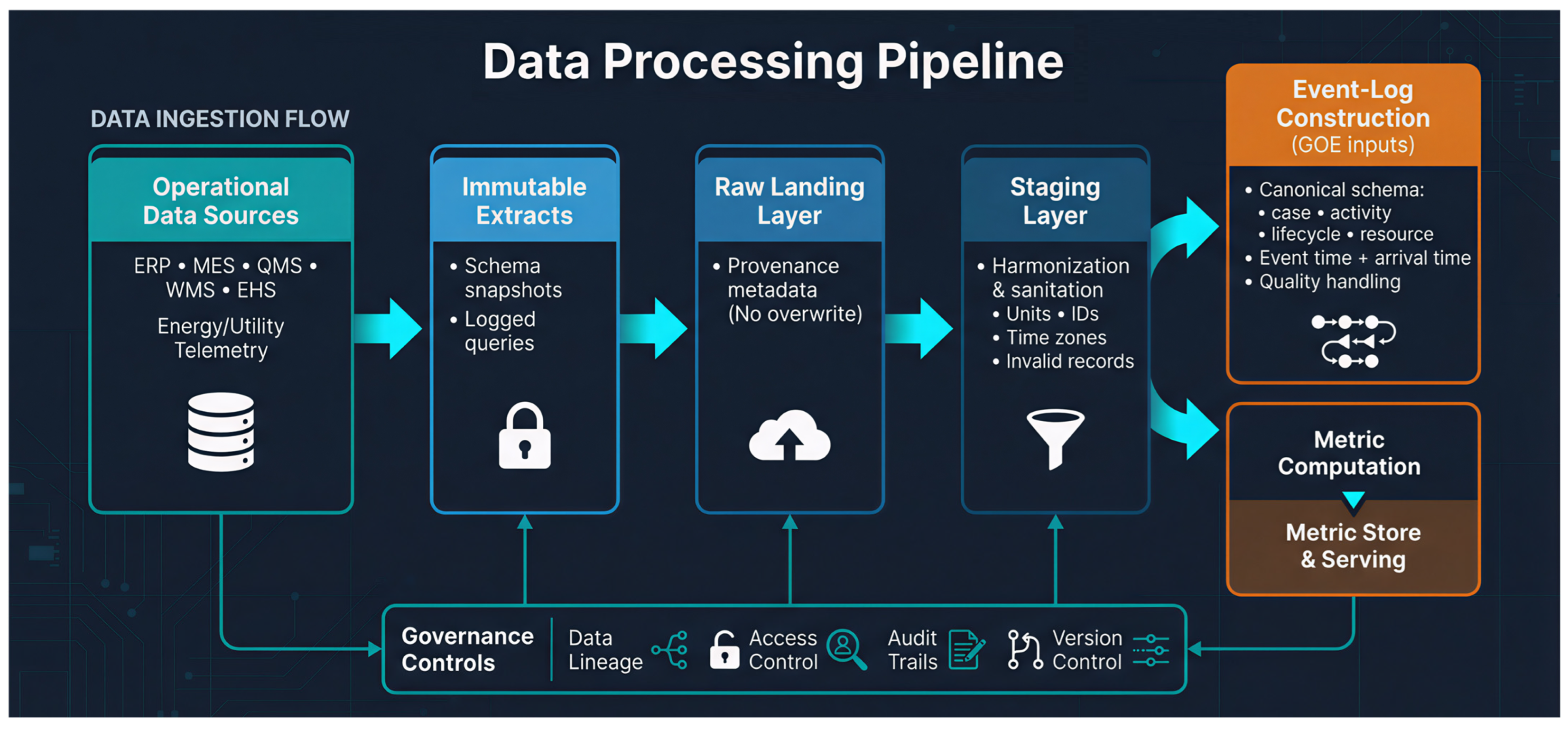
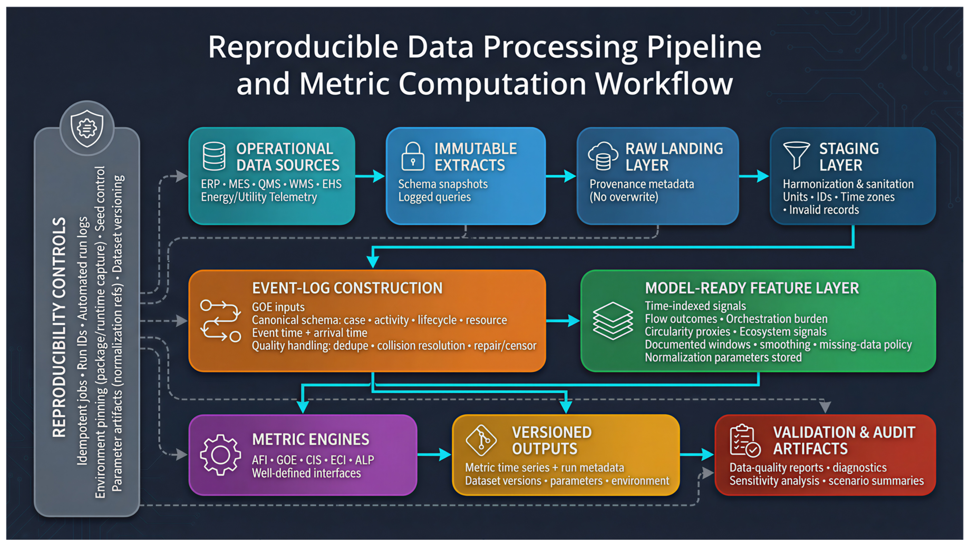
GOE is computed from event logs and, therefore, requires an explicit event-log quality management procedure to ensure that the inferred value stream is not an artifact of timestamp imperfections, incompleteness, or noise. Event-log preprocessing is treated as a mandatory upstream step because missing, duplicate, erroneous, and noisy records are known to materially distort process-mining outputs and performance inferences if left unaddressed [58]. Timestamp quality is treated as especially consequential because missing, incorrect, or coarse-granularity timestamps can alter event ordering and thereby bias any time-indexed performance measurement derived from the log [59].

For timestamp collisions (events recorded with identical timestamps, often due to limited ERP/MES timestamp granularity or asynchronous write behavior), the log is first normalized to a canonical time basis (timezone unification, clock-skew correction when multi-system sources exist, and removal of impossible time regressions). Collisions are then resolved using a deterministic tie-breaking rule that is auditable and reproducible: lifecycle ordering (e.g., start before complete where available), system commit sequence numbers or monotonically increasing event identifiers, and, when present, source-system precedence rules that reflect the actual write path. When no reliable secondary ordering attribute exists, the affected events are treated as concurrent and the induced uncertainty is carried into GOE rather than being hidden by arbitrary ordering; concretely, the within-timestamp order is sampled across admissible permutations, and GOE is reported as an expected value with a dispersion band over those permutations. This treatment aligns with established process-data quality practice that emphasizes detection, quantification, and repair of timestamp imperfections before downstream inference, and it is consistent with published methods specifically designed to repair identical timestamp errors in event logs [60].

For missing logs (missing activities, missing lifecycle transitions, or missing timestamps), the log is subjected to completeness diagnostics prior to GOE computation. Completeness is assessed at both the trace level (whether a case contains the minimal required milestones for value-stream inference) and the event level (whether expected intermediate steps are absent). Missingness is detected using a combination of (i) invariant constraints derived from the process definition when such constraints exist (e.g., required predecessor/successor relations) and (ii) conformance-based diagnostics when a normative process model or reference process skeleton is available. When repair is defensible, missing events are imputed using model-based repair procedures that infer likely missing segments while preserving resource constraints and inter-case dependencies; this is consistent with the process-mining literature on repairing event logs with missing events to support performance analysis [61]. When repair is not defensible (e.g., missingness is extensive or structurally ambiguous), the affected traces are treated as censored rather than “completed” by assumption: GOE is computed on the observed prefix, and the reporting includes a coverage factor (fraction of required milestones observed within the GOE horizon) so that low-completeness periods are not mistakenly interpreted as efficiency changes.

For phantom events (duplicate records, spurious system-generated events that do not correspond to real process executions, and noise events), the pipeline applies a staged filtering and deduplication procedure. Exact duplicates are removed using a strict key match on (case_id, activity, timestamp, resource, lifecycle) when available, and near-duplicates are removed using a short temporal tolerance window when ERP/MES systems are known to emit repeated writes. Noise and phantom events are detected by rule-based and statistical criteria: activity labels that are irrelevant to the value-stream definition, impossible transitions under the process constraints, and extreme-duration anomalies that indicate instrumentation errors. This aligns with the established view that low-quality logs containing duplicates, irrelevant events, and noise must be corrected or filtered to prevent distorted models and misleading performance conclusions [62]. The filtering thresholds are treated as governed parameters and are included in the same sensitivity-audit logic used elsewhere in the manuscript, because repair and filtering choices can alter downstream metrics if they are not explicitly controlled.

4.3. Pillar 3: Circular–Regenerative Analytics

Definition: This pillar elevates sustainability from an external constraint to a core, coequal objective of the Lean system [63]. It integrates the principles of the circular economy and regenerative design into a new set of analytical tools and metrics, moving far beyond the often superficial “Green Lean” initiatives.

Theoretical Grounding: This pillar is based on the theory of the circular economy [64,65,66] and the emerging concept of regenerative design. It operationalizes the vision of a sustainable I6.0 [67,68].

Key Principles and Extension of Lean:

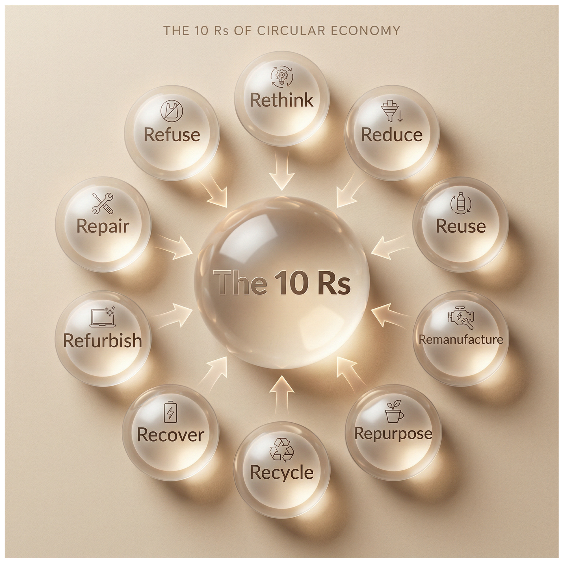
• The “10 Rs” of Lean: The traditional “3Rs” of sustainability (Reduce, Reuse, Recycle) are expanded to a more comprehensive set of circular economy principles, which are treated as core Lean objectives. These include Refuse, Rethink, Reduce, Reuse, Repair, Refurbish, Remanufacture, Repurpose, Recycle, and Recover. The I6LA Framework provides metrics for each of these “10 Rs,” allowing them to be integrated into a holistic measure of circularity (see Figure 8).
• Real-Time Life Cycle Assessment (LCA): Traditional LCA is a time-consuming, offline process. The I6LA framework proposes the use of digital twins and real-time data from IoT sensors to perform LCA dynamically, as products are being designed and manufactured. This would allow the GAI orchestrator to make real-time trade-offs between production efficiency and life cycle impact, for example, by choosing a slightly more expensive but more easily recyclable material.
• Value Stream Mapping for Circularity (VSM-C): A new form of VSM is proposed that maps not just the flow of materials and information in the forward supply chain, but also the reverse loops of the circular economy. VSM-C would visualize the flow of used products, components, and materials back into the production system, identifying wastes and opportunities in the reverse logistics, remanufacturing, and recycling processes.

4.3.1. Circularity Integration Score (CIS)

The CIS is defined as a single, bounded index that embeds three requirements as coequal mathematical components: (i) operationalization of the circular “10R” strategy set as measurable execution rates, consistent with contemporary circular-economy scholarship that frames circularity as a system-level shift across supply chains rather than a narrow end-of-life intervention; (ii) real-time environmental performance measured through a dynamic life-cycle impact model continuously updated via digital twin and IoT data feeds, which is the enabling mechanism for “dynamic” or near real-time Life Cycle Assessment (LCA) rather than offline, static assessments; and (iii) a value-stream representation that explicitly includes reverse loops (collection, reuse, repair, refurbish, remanufacture, recycle, recovery) as first-class flow paths, consistent with adaptations of VSM to circular systems and with circular VSM formulations that integrate I4.0 data streams and circular-economy practices. A regenerative extension is included as a distinct term that captures “net-positive” contributions (i.e., improvements that go beyond harm reduction), consistent with recent regenerative-systems theory emphasizing reinforcing cycles of wellbeing and systemic vitality (see

Table A3. CIS symbols and units (Pillar 3).

Symbol	Meaning	Units
CIS(t)	Circularity Integration Score	dimensionless (0–1)
SR(t), SL(t), SV(t), SG(t)	Component scores (10R, real-time LCA, VSM-C, regenerative surplus)	dimensionless (0–1)
wR, wL, wV, wG	Component weights	dimensionless (sum to 1)
ε	Stability constant	dimensionless
T	Evaluation horizon length	epochs or time (as implemented)
CIS(0:T)	Horizon-level discounted CIS	dimensionless
r	10R strategy index	dimensionless (index)
p	Product family/SKU index	dimensionless (index)
$\mathcal{P}$	Set of monitored products	set
E(p,r,t)	Eligible units/mass for strategy r	count or mass
U(p,r,t)	Units/mass handled under strategy r	count or mass
δ	Nonzero denominator constant	same as denominator quantity
φ(p,r,t)	Product-level realization rate	dimensionless
ωp	Portfolio weight	dimensionless
φr(t)	Portfolio realization rate for strategy r	dimensionless
ρr	Strategy weights within 10R component	dimensionless
SR(raw,t)	Raw 10R score	dimensionless
F(p,r,t)	Feasibility indicator	dimensionless (0/1)
Mp(t)	Misallocation mass/volume proxy	count or mass
μ(t)	Misallocation rate proxy	dimensionless
ΠR(t)	Dominance/feasibility penalty	dimensionless (0–1)
SR(t)	Final 10R component	dimensionless (0–1)
c	Impact-category index	dimensionless (index)
j	Elementary flow index	dimensionless (index)
J	Number of elementary flows	count
C	Number of impact categories	count
ej(t)	Measured elementary flow j	flow units (e.g., kg, kWh)
CF(j,c)	Characterization factor	impact units per flow unit
Ic(t)	Dynamic impact in category c	category units (e.g., kg CO2-eq)
Iref,c; Ibest,c	Reference and best/target impacts	same as Ic(t)
sc(t)	Normalized impact score	dimensionless (0–1)
βc	Impact-category weights	dimensionless
SL(t)	Aggregated LCA component	dimensionless (0–1)
qim(t)	Material flow rate from node i to m	mass/time or count/time
$\mathcal{N}$	Node set in value-network graph	set
m	Manufacturing node identifier	identifier
Erev	Reverse-loop edge set	set
Qin(t), Qsec(t)	Inbound and secondary inbound flows	same as q
LCR(t)	Loop-closure rate Qsec/Qin	dimensionless
c (customer)	Customer node index (contextual)	identifier
Qret(t), Qusable(t)	Returned flow and usable reintegrated input	same as q
RY(t)	Reverse yield Qusable/Qret	dimensionless
RLT(t)	Reverse lead time	time
RLTref, RLTbest	Reference/target reverse lead time	time
RT(t)	Reverse-time score	dimensionless (0–1)
αLcR, αRy, αRT	VSM-C aggregation weights	dimensionless
SV(t)	VSM-C component	dimensionless (0–1)
gc(t)	Regenerative credit in category c	same as category units
NPc(t)	Net-positive surplus max{0, gc(t) − Ic(t)}	category units
${\mathrm{N}\mathrm{P}}_c^{\mathrm{t}\mathrm{a}\mathrm{r}\mathrm{g}}$	Target net-positive surplus	category units
uc(t)	Bounded surplus score	dimensionless (0–1)
SG(t)	Regenerative component	dimensionless (0–1)

in Appendix A for all related mathematical symbols).

CIS is derived from an explicit design axiom that sustainability is not an external constraint but a coequal Lean objective; therefore, the aggregation rule must be non-compensatory in the sense that poor circularity performance cannot be fully offset by strong performance in a different sustainability dimension. This axiom is satisfied by a weighted geometric mean (equivalently, an exponentiated weighted log-sum), because the geometric mean penalizes any component approaching zero and yields zero when any required component is zero. Let the four component scores at time $t$ be $S_R(t)$ (10R execution), $S_L(t)$ (real-time LCA performance), $S_V(t)$ (VSM for circularity, including reverse loops), and $S_G(t)$ (regenerative surplus). Each component is explicitly normalized to $\left[0,1\right]$. Let $\mathrm{w}=(w_R,w_L,w_V,w_G)\in {\Delta }^3$ be nonnegative weights summing to one. Let $ϵ\in (0,1)$ be a small numerical constant ensuring numerical stability when a component is exactly zero. The instantaneous CIS is defined as

$$\mathrm{C}\mathrm{I}\mathrm{S}(t)=\mathrm{e}\mathrm{x}\mathrm{p}(w_R\mathrm{l}\mathrm{n}(S_R(t)+ϵ)+w_L\mathrm{l}\mathrm{n}(S_L(t)+ϵ)+w_V\mathrm{l}\mathrm{n}(S_V(t)+ϵ)+w_G\mathrm{l}\mathrm{n}(S_G(t)+ϵ)).$$

(30)

Thus, $\mathrm{C}\mathrm{I}\mathrm{S}(t)\in (0,1+ϵ)$ and, for sufficiently small $ϵ$, it behaves as a weighted geometric mean on $\left[0,1\right]$. Over an evaluation horizon $t\in \{0,1,\dots ,T\}$, with a discount factor $\left.\gamma \in (0,1\right]$, the horizon-level CIS is defined as the normalized discounted average:

$${\mathrm{C}\mathrm{I}\mathrm{S}}_{0:T}={\displaystyle \frac{{\sum }_{t=0}^T{\gamma }^t \mathrm{C}\mathrm{I}\mathrm{S}(t)}{{\sum }_{t=0}^T{\gamma }^t}}.$$

(31)

The remainder of the derivation consists of defining $S_R(t)$, $S_L(t)$, $S_V(t)$, and $S_G(t)$ from measurable quantities in an I6.0 setting.

The 10R execution component $S_R(t)$ formalizes the “10 Rs” as measurable rates at the product-portfolio level. Let $\mathcal{R}=\{0,1,\dots ,9\}$ index the ten strategies, where $r=0$ corresponds to Refuse and $r=9$ corresponds to Recover. Let $\mathcal{P}$ be the set of product families (or SKUs) monitored. For each product $p\in \mathcal{P}$ and strategy $r\in \mathcal{R}$, let $E_{p,r}(t)\in {\mathbb{R}}_{\ge 0}$ denote the number of eligible units (or eligible mass) for which strategy $r$ could be applied during the monitoring interval ending at $t$; eligibility is determined by engineering feasibility and business rules (e.g., a repairable component is eligible for Repair). Let $U_{p,r}(t)\in {\mathbb{R}}_{\ge 0}$ denote the number of units (or mass) actually handled under strategy $r$ during the same interval. The product-level realization rate is

$${\varphi }_{p,r}\left(t\right)={\displaystyle \frac{U_{p,r}\left(t\right)}{\max \left\{E_{p,r}\left(t\right),\delta \right\}}},$$

(32)

where $\delta >0$ is a small constant preventing division by zero when eligibility is absent. Let ${\omega }_p\ge 0$ be a portfolio weight for product $p$, with ${\sum }_{p\in \mathcal{P}}{\omega }_p=1$; ${\omega }_p$ can be proportional to production volume, revenue share, or criticality. The portfolio-level realization rate for the strategy $r$ is

$${\varphi }_r(t)={\sum }_{p\in \mathcal{P}}{\omega }_p {\varphi }_{p,r}(t).$$

(33)

Because the 10R framework is hierarchical (higher-order strategies are typically preferable to lower-order end-of-life strategies), a strategy-importance weight vector $\rho =({\rho }_0,\dots ,{\rho }_9)\in {\Delta }^9$ is introduced, where ${\rho }_r\ge 0$ and ${\sum }_{r=0}^9{\rho }_r=1$. The integration of R-strategy indicators using structured weighting approaches (e.g., AHP) to form a unified circularity index, motivating $\rho$ as an explicit, auditable design choice rather than an implicit preference. The raw 10R score is then

$$S_R^{\mathrm{r}\mathrm{a}\mathrm{w}}(t)={\sum }_{r=0}^9{\rho }_r {\varphi }_r(t).$$

(34)

To prevent superficial inflation of circularity through excessive reliance on lower-priority strategies when higher-priority strategies are feasible, a dominance-violation penalty is defined. Let $F_{p,r}\left(t\right)\in \left\{0,1\right\}$ indicate whether the product $p$ is feasible for the strategy $r$ at time $t$ (as determined by design, condition monitoring, and policy). Let $r<q$ denote that strategy $r$ is hierarchically preferred to $q$. Let $U_{p,q}(t)$ be the quantity assigned to the lower strategy $q$. The misallocation mass for the product $p$ is defined as

$$M_p(t)=\sum _{q=0}^9(U_{p,q}(t)\cdot 1\{\exists r<q \mathrm{such} \mathrm{that} F_{p,r}(t)=1\}),$$

(35)

which counts units sent to a lower strategy while a higher strategy was feasible. Let $U_p(t)={\sum }_{q=0}^9{U}_{p,q}(t)$ be the total circular-handling volume for $p$. The portfolio-level misallocation rate is

$$\mu (t)={\sum }_{p\in \mathcal{P}}{\omega }_p {\displaystyle \frac{M_p(t)}{\mathrm{m}\mathrm{a}\mathrm{x}\{U_p(t),\delta \}}}.$$

(36)

A bounded penalty factor is then defined as ${\mathrm{\Pi }}_R(t)=\mathrm{e}\mathrm{x}\mathrm{p}(-{\kappa }_R \mu (t))$, where ${\kappa }_R\ge 0$ controls strictness. The final 10R execution component is

$$S_R(t)=\mathrm{c}\mathrm{l}\mathrm{i}\mathrm{p}(S_R^{\mathrm{r}\mathrm{a}\mathrm{w}}(t)\cdot {\mathrm{\Pi }}_R(t), 0, 1),$$

(37)

where $\mathrm{c}\mathrm{l}\mathrm{i}\mathrm{p}(x,0,1)=\mathrm{m}\mathrm{i}\mathrm{n}\{1,\mathrm{m}\mathrm{a}\mathrm{x}\{0,x\}\}$. This construction ensures that “Green Lean” actions that merely shift waste to lower-value loops do not receive unearned credit.

The real-time LCA component $S_L(t)$ is derived from a dynamic life-cycle impact model parameterized by continuously updated digital twin measurements. Let $j\in \{1,\dots ,J\}$ index elementary flows (e.g., electricity consumption, fuel use, CO₂ emissions, particulate matter, water withdrawal), and let $c\in \{1,\dots ,C\}$ index impact categories (e.g., climate change, water scarcity). Let $e_j(t)\in {\mathbb{R}}_{\ge 0}$ be the measured quantity of elementary flow $j$ attributable to the system during the monitoring interval ending at $t$, obtained from IoT sensors and the manufacturing digital twin. Let ${\mathrm{C}\mathrm{F}}_{j,c}\in {\mathbb{R}}_{\ge 0}$ be the characterization factor mapping elementary flow $j$ to impact category $c$. The dynamic impact in category $c$ is

$$I_c(t)={\sum }_{j=1}^J{\mathrm{C}\mathrm{F}}_{j,c} e_j(t).$$

(38)

Let $I_c^{\mathrm{r}\mathrm{e}\mathrm{f}}>0$ be a reference (baseline) impact level for category $c$, and let $I_c^{\mathrm{b}\mathrm{e}\mathrm{s}\mathrm{t}}\ge 0$ be a best-achievable or target impact for category $c$ under current technology constraints, with $I_c^{\mathrm{b}\mathrm{e}\mathrm{s}\mathrm{t}}<I_c^{\mathrm{r}\mathrm{e}\mathrm{f}}$. A normalized improvement score is defined as

$$s_c\left(t\right)=\mathrm{c}\mathrm{l}\mathrm{i}\mathrm{p}\left({\displaystyle \frac{I_c^{\mathrm{r}\mathrm{e}\mathrm{f}}-I_c\left(t\right)}{I_c^{\mathrm{r}\mathrm{e}\mathrm{f}}-I_c^{\mathrm{b}\mathrm{e}\mathrm{s}\mathrm{t}}}}, 0, 1\right).$$

(39)

Let $\beta =({\beta }_1,\dots ,{\beta }_C)\in {\Delta }^{C-1}$ be impact-category weights (policy- or stakeholder-defined). The real-time LCA component becomes

$$S_L(t)={\sum }_{c=1}^C{\beta }_c s_c(t)\in [0,1].$$

(40)

This definition makes sustainability a coequal objective by converting multi-category impacts into a bounded performance term that can neither be ignored nor relegated to a side constraint.

The VSM-for-circularity component $S_V(t)$ is derived from a value-stream representation that includes reverse flows and their operational wastes (time, losses, leakage from loops). Let the circular value-stream network contain nodes $\mathcal{N}$ (e.g., suppliers, manufacturing, customers, collection, inspection/sorting, repair, refurbish, remanufacture, recycling, recovery, disposal). Let directed arcs be $(i,j)\in \mathcal{E}\subseteq \mathcal{N}\times \mathcal{N}$. Let $q_{ij}(t)\in {\mathbb{R}}_{\ge 0}$ denote the measured mass-flow rate (or unit-flow rate) from node $i$ to node $j$ during the monitoring interval ending at $t$, derived from ERP/MES logs, logistics telemetry, and digital twin tracking. Let ${\mathcal{E}}_{\mathrm{r}\mathrm{e}\mathrm{v}}\subseteq \mathcal{E}$ denote reverse-loop arcs (customer-to-collection, collection-to-repair, repair-to-manufacturing, recycling-to-manufacturing, etc.). Let manufacturing be indexed by node $m\in \mathcal{N}$, and let inert input be represented by a source node $v\in \mathcal{N}$. Define total inbound material to manufacturing as

$$Q^{\mathrm{i}\mathrm{n}}\left(t\right)=\sum _{i\in \mathcal{N}}{q}_{im}\left(t\right),$$

(41)

And secondary inbound (from reverse loops) as

$$Q^{\mathrm{s}\mathrm{e}\mathrm{c}}\left(t\right)=\sum _{i:\left(i,m\right)\in {\mathcal{E}}_{\mathrm{r}\mathrm{e}\mathrm{v}}}{q}_{im}\left(t\right),$$

(42)

then, inert inbound as $Q^{\mathrm{v}\mathrm{i}\mathrm{r}}(t)=q_{vm}(t)$ (or the appropriate sum of inert-supply arcs). The loop-closure rate is

$$\mathrm{L}\mathrm{C}\mathrm{R}\left(t\right)={\displaystyle \frac{Q^{\mathrm{s}\mathrm{e}\mathrm{c}}\left(t\right)}{\max \left\{Q^{\mathrm{i}\mathrm{n}}\left(t\right),\delta \right\}}},$$

(43)

which measures the extent to which production is being fed by returned or recovered streams rather than inert extraction. Let $Q^{\mathrm{r}\mathrm{e}\mathrm{t}}(t)$ be the total returns entering the reverse network from customers, defined as

$$Q^{\mathrm{r}\mathrm{e}\mathrm{t}}(t)={\sum }_{j:(c,j)\in {\mathcal{E}}_{\mathrm{r}\mathrm{e}\mathrm{v}}}{q}_{cj}(t),$$

(44)

where $c$ denotes the customer node(s). Let $Q^{\mathrm{u}\mathrm{s}\mathrm{a}\mathrm{b}\mathrm{l}\mathrm{e}}(t)=Q^{\mathrm{s}\mathrm{e}\mathrm{c}}(t)$ be the reverse material that becomes usable manufacturing input. The reverse-yield is

$$\mathrm{R}\mathrm{Y}\left(t\right)={\displaystyle \frac{Q^{\mathrm{u}\mathrm{s}\mathrm{a}\mathrm{b}\mathrm{l}\mathrm{e}}\left(t\right)}{\max \left\{Q^{\mathrm{r}\mathrm{e}\mathrm{t}}\left(t\right),\delta \right\}}}.$$

(45)

To incorporate time waste in reverse loops (a central purpose of VSM-Circularity), let $\mathrm{R}\mathrm{L}\mathrm{T}\left(t\right)\ge 0$ be the measured mean reverse lead time from customer return to reintegration into manufacturing input, computed from trace timestamps in the digital twin and logistics logs. Let ${\mathrm{R}\mathrm{L}\mathrm{T}}^{\mathrm{r}\mathrm{e}\mathrm{f}}>0$ be a reference reverse lead time and ${\mathrm{R}\mathrm{L}\mathrm{T}}^{\mathrm{b}\mathrm{e}\mathrm{s}\mathrm{t}}\ge 0$ be a target. A bounded reverse-time score is

$$\mathrm{R}\mathrm{T}\left(t\right)=\mathrm{c}\mathrm{l}\mathrm{i}\mathrm{p}\left({\displaystyle \frac{{\mathrm{R}\mathrm{L}\mathrm{T}}^{\mathrm{r}\mathrm{e}\mathrm{f}}-\mathrm{R}\mathrm{L}\mathrm{T}\left(t\right)}{{\mathrm{R}\mathrm{L}\mathrm{T}}^{\mathrm{r}\mathrm{e}\mathrm{f}}-{\mathrm{R}\mathrm{L}\mathrm{T}}^{\mathrm{b}\mathrm{e}\mathrm{s}\mathrm{t}}}}, 0, 1\right).$$

(46)

The VSM-C component is then constructed as a weighted aggregation of closure, yield, and reverse-time performance:

$$S_V(t)={\alpha }_{\mathrm{L}\mathrm{C}\mathrm{R}} \mathrm{L}\mathrm{C}\mathrm{R}(t)+{\alpha }_{\mathrm{R}\mathrm{Y}} \mathrm{R}\mathrm{Y}(t)+{\alpha }_{\mathrm{R}\mathrm{T}} \mathrm{R}\mathrm{T}(t),$$

(47)

where ${\alpha }_{\mathrm{L}\mathrm{C}\mathrm{R}},{\alpha }_{\mathrm{R}\mathrm{Y}},{\alpha }_{\mathrm{R}\mathrm{T}}\ge 0$ and ${\alpha }_{\mathrm{L}\mathrm{C}\mathrm{R}}+{\alpha }_{\mathrm{R}\mathrm{Y}}+{\alpha }_{\mathrm{R}\mathrm{T}}=1$. This ensures that circularity is not credited merely by collecting returns; the reverse system must also convert returns into usable inputs and do so with low lead-time waste.

The regenerative component $S_G(t)$ is derived to capture performance that goes beyond impact reduction and loop closure by explicitly crediting net-positive contributions. Let $g_c(t)\in {\mathbb{R}}_{\ge 0}$ denote a measured regenerative credit in category $c$ during the monitoring interval ending at $t$ (e.g., verified sequestration, verified restoration activity quantified in the same category units, or verified ecosystem-service proxies), obtained through certified measurements or validated digital twin modules. Regenerative systems theory emphasizes reinforcing cycles of wellbeing and systemic vitality; therefore, the regenerative term is defined as a surplus beyond neutral performance rather than as a mere reduction in harms. Thus, the net-positive surplus in category $c$ is defined as

$${\mathrm{N}\mathrm{P}}_c\left(t\right)=\max \left\{0, g_c\left(t\right)-I_c\left(t\right)\right\},$$

(48)

where $I_c(t)$ is the dynamic impact already defined in the LCA component. Let ${\mathrm{N}\mathrm{P}}_c^{\mathrm{t}\mathrm{a}\mathrm{r}}>0$ be a target net-positive surplus for category $c$. A bounded surplus score is

$$u_c\left(t\right)=\mathrm{c}\mathrm{l}\mathrm{i}\mathrm{p}\left({\displaystyle \frac{{\mathrm{N}\mathrm{P}}_c\left(t\right)}{{\mathrm{N}\mathrm{P}}_c^{\mathrm{t}\mathrm{a}\mathrm{r}}}}, 0, 1\right).$$

(49)

Using the same category weight vector $\beta$ for consistency of sustainability valuation, the regenerative component is defined as

$$S_G(t)={\sum }_{c=1}^C{\beta }_c u_c(t)\in [0,1].$$

(50)

This construction yields $S_G(t)=0$ when regenerative surplus is absent and increases only when measured net-positive performance exceeds measured life-cycle burdens in one or more categories.

Substituting the fully defined component scores into the aggregation rule gives the complete CIS expression. The definition is intentionally non-compensatory: because $\mathrm{C}\mathrm{I}\mathrm{S}(t)$ is a weighted geometric mean (with stability constant $ϵ$), any failure in one pillar element (e.g., negligible reverse-loop reintegration such that $S_V(t)\approx 0$, or absent 10R execution such that $S_R(t)\approx 0$) suppresses the overall CIS even if another element is strong, thereby mathematically implementing the pillar’s stated objective that sustainability is a core, coequal Lean objective rather than a peripheral “green” add-on.

Mathematical Impact

CIS uses a weighted geometric mean specifically to enforce non-compensatory behavior, meaning that weak circularity dimensions are intended to dominate the score rather than being offset by strong dimensions. The stability constant $ϵ$ is introduced only to prevent numerical becoming undefined when a component approaches zero; however, $ϵ$ necessarily modifies boundary behavior and therefore must be governed and reported [69].

When any CIS component is exactly zero, the presence of $ϵ$ implies that the CIS is not forced to zero; instead, it attains a small positive value whose magnitude is determined by $ϵ$ and the weight assigned to the zero component. The practical implication is that $ϵ$ induces a non-zero “floor,” and the floor increases as $ϵ$ increases. Conversely, if $ϵ$ is made very small, CIS becomes highly sensitive to tiny changes in near-zero components: very small improvements (or small measurement noise) in the weakest dimension can cause disproportionately large changes in CIS. Therefore, $ϵ$ governs a tradeoff between numerical stability and boundary sensitivity, and it is not a purely technical detail [70].

To ensure valid scoring, $ϵ$ is specified as a governed constant tied to measurement resolution rather than selected arbitrarily. It is set relative to the smallest reliably detectable positive increment of the normalized component scale after preprocessing. Under this rule, $ϵ$ remains small enough that the induced floor is negligible for substantive interpretation, while still preventing numerical issues. In addition, a distinction is enforced between structural zeros and measurement zeros. A structural zero represents a genuine absence of capability in an essential circularity dimension and should yield a CIS of zero by definition. $ϵ$ is not permitted to convert that absence into a non-zero score. A measurement zero arises from censoring, missingness, rounding, or proxy limitations and is handled through explicit data-quality procedures rather than being treated as substantive performance [71].

To prevent baseline drift from being misclassified as regenerative improvement, the framework differentiates two drivers of change: (i) changes in the burden term $I_c(t)$ caused by dynamic external conditions captured by the dynamic LCA model (e.g., time-varying grid intensity, supplier background changes, time-dependent characterization factors), and (ii) changes in the credit term $R_c(t)$ attributable to additional, verifiable regenerative actions. Dynamic LCA is explicitly designed to represent temporal variation in both foreground flows and background systems, and, therefore, drift in $I_c(t)$ is treated as a measured, time-indexed quantity rather than an unmodeled disturbance [72]. The implication is that a reduction in $I_c(t)$ arising from external decarbonization of the grid (or similar background shifts) is recorded as a change in burden, not as regenerative surplus, unless the credit term independently increases beyond what the baseline allows.

The separation between genuine regeneration and external drift is enforced through two governance rules. First, $I_c(t)$ is computed using time-indexed background and characterization updates (e.g., grid mix and other background inventories) so that exogenous drift is absorbed into the burden measurement rather than implicitly credited to regeneration; this directly addresses the drift mechanism and aligns with established concerns about temporal variability in electricity and background systems in LCA [73]. Second, $R_c(t)$ is defined as a verified regenerative credit with explicit additionality and baseline specification, meaning that credits are admissible only when they exceed a declared baseline scenario and satisfy monitoring, reporting, and verification constraints. This requirement prevents “credits” from reflecting favorable external trends or accounting artifacts and aligns with the literature documenting baseline manipulation and additionality weaknesses in offset and crediting systems [74].

Neutral performance in the category $c$ is represented by the contemporaneous dynamic burden $I_c(t)$ under the declared system boundary, while net-positive performance requires the additional, verified credit stream $R_c(t)$ to exceed that burden. To make attribution explicit, reporting includes a decomposition showing whether changes in net-positive surplus over time arise primarily from (a) reductions in $I_c(t)$ driven by background drift (e.g., grid decarbonization) or (b) increases in $R_c(t)$ driven by verified regenerative interventions. Under this reporting rule, genuine regenerative improvement is declared only when the surplus is positive and is supported by admissible credits defined relative to an explicit baseline, whereas improvements caused by external drift remain classified as burden variation within $I_c(t)$ rather than being reclassified as regeneration.

4.4. Pillar 4: Hyper-Connected Ecosystem Integration

Definition: This pillar provides the analytical tools to manage and optimize performance across the vast, hyper-connected ecosystems of I6.0. It extends the unit of analysis for Lean from the single factory or supply chain to the entire, dynamic network of suppliers, partners, customers, and even products in the field 9 (see Figure 9).

Theoretical Grounding: This pillar is based on the vision of a hyper-connected I6.0 [75,76,77]. It draws on concepts from network theory [78], systems engineering, industrial data sharing [79], and platform economics to provide a framework for ecosystem-level analysis [80,81,82].

Key Principles:

• Ecosystem-Level Kaizen: The concept of Kaizen is applied to the entire ecosystem. The framework includes mechanisms for identifying and eliminating “ecosystem wastes” such as information asymmetry between partners, data friction at system interfaces, misaligned incentives, and delays caused by a lack of trust. This requires a new level of inter-organizational collaboration and data sharing.
• The “Metaverse Gemba”: Building on the Digital Gemba, the Metaverse Gemba is a shared, persistent virtual space where all stakeholders in the ecosystem (e.g., suppliers, logistics providers, customers, maintenance partners) can interact with a live digital twin of the entire value network. This enables a new form of collaborative problem-solving, where a supplier in one country can work with an engineer in another to diagnose and fix a problem in a factory in a third country, all within a shared virtual environment.
• Information Flow as a Utility: The framework treats information flow not as a series of discrete transactions, but as a continuous, utility-like service that must be optimized for quality, latency, security, and cost across the entire ecosystem. This requires a new set of metrics and analytical tools focused on the health and performance of the underlying data fabric that connects the ecosystem.

Ecosystem Connectivity Index (ECI)

ECI is defined as a single, bounded metric that quantifies the operational “connectedness” of an I6.0 ecosystem as a networked utility system, rather than as a set of bilateral transactions. The index is constructed so that it (i) measures the structural capacity of the ecosystem to remain connected and coorientable under dynamic conditions, (ii) measures the quality, security, and interoperability of the information fabric as a continuous service, (iii) measures shared observability and collaborative controllability through a metaverse-grade digital twin space, and (iv) measures the rate at which ecosystem wastes (information asymmetry, data friction, misaligned incentives, trust delays) are identified and reduced via ecosystem-level Kaizen. This framing is consistent with I6.0 emphasizing hyper-connectivity, metaverse-assisted virtual production, and pervasive digital twins, and with the view that inter-organizational data spaces and interoperability are foundational for cross-firm orchestration (see

Table A4. ECI symbols and units (Pillar 4).

Symbol	Meaning	Units
$\mathcal{G}$t = ($\mathcal{V}$, $\mathcal{\epsilon }$t)	Information-fabric graph at epoch t	graph object
$\mathcal{V}$	Stakeholder node set	set/count
n	Number of nodes	count
i, j	Node indices	dimensionless (indices)
Lij(t)	End-to-end latency	seconds
Bij(t)	Usable throughput	bits/s or messages/s
Aij(t)	Availability	dimensionless fraction
Pij(t)	Success probability	dimensionless probability
Σij(t)	Security score	dimensionless (0–1)
Iij(t)	Semantic interoperability score	dimensionless (0–1)
Kij(t)	Marginal service cost	$/GB or $/message
Lref, Bref, Kref	Reference scales	seconds; bits/s (or msg/s); $/GB (or $/msg)
uLij(t), uBij(t), uKij(t)	Normalized utilities (latency/throughput/cost)	dimensionless (0–1)
uAij(t), uPij(t), u^Σij(t), uIij(t)	Normalized utilities (availability/success/security/interoperability)	dimensionless (0–1)
αL, αB, αA, αP, α^Σ, αI, αK	Attribute weights in edge-utility aggregation	dimensionless (sum to 1)
Uij(t)	Edge utility	dimensionless (0–1)
wij(t)	Effective information-carrying capacity/edge weight	throughput units scaled by utility
SU(t)	Ecosystem information-utility score	dimensionless (0–1)
W(t)	Symmetrized effective-weight matrix	same as wij
di(t)	Node degree in the symmetrized weighted graph	same as wij
D(t)	Degree matrix diag(di)	same as wij
L(t)	Weighted Laplacian L = D − W	same as wij
λ2(t)	Algebraic connectivity (Fiedler value)	same as wij
Wtot(t)	Total undirected weight budget	same as wij
SC(t)	Normalized structural connectivity score	dimensionless (0–1)
ntwin(t)	Nodes with active live digital twin	count
Ccov(t)	Twin coverage fraction ntwin/n	dimensionless (0–1)
Δsync(t)	Synchronization lag	time
Δref	Reference lag scale	time
Csync(t)	Synchronization score exp(−Δsync/Δref)	dimensionless (0–1)
nactive(t)	Nodes actively participating	count
Cpart(t)	Participation fraction nactive/n	dimensionless (0–1)
Ninc(≤τ)	Incidents resolved within threshold τ	count
Ninc(t)	Total incidents observed	count
Cres(t)	Resolution fraction	dimensionless (0–1)
βcov, βsync, βpart, βres	Metaverse Gemba weights	dimensionless (sum to 1)
SM(t)	Metaverse/Digital-Gemba observability score	dimensionless (0–1)
p(i·,t), p(·,t)	Belief distributions used in divergence term	dimensionless probability vectors
A(t)	Information-asymmetry divergence magnitude	dimensionless
Aref	Reference scale for asymmetry normalization	dimensionless
SA(t)	Asymmetry health score exp(−A/Aref)	dimensionless (0–1)
Nman(t)	Manual interventions	count
Ntx(t)	Traceability transactions/records	count
Ft	Friction ratio Nman/max{Ntx,1}	dimensionless
Fref	Reference friction scale	dimensionless
SF(t)	Friction health score exp(−F/Fref)	dimensionless (0–1)
rtaui, rtauE	Local/ecosystem traces used in misalignment proxy	trace-dependent
Mmis(t)	Misalignment magnitude	dimensionless
Mref	Reference misalignment scale	dimensionless
SMis(t)	Misalignment health score exp(−Mmis/Mref)	dimensionless (0–1)
$\mathcal{Q}$t	Query/task set for trust-delay waste	set
τapp,φ; τreφ,φ	Achieved/requested times	time
Dwaste(t)	Trust-delay waste proxy	time
Dref	Reference delay scale	time
SD(t)	Delay health score exp(−Dwaste/Dref)	dimensionless (0–1)
ηA, ηf, ηMis, ηD	Weights in the ecosystem waste score	dimensionless (sum to 1)
SW(t)	Ecosystem-waste reduction score	dimensionless (0–1)
Ωt	Waste potential −ln(SW(t)+ε)	dimensionless
ΔΩt	Change in waste potential	dimensionless
ΔΩref	Reference scale for Kaizen normalization	dimensionless
SK(t)	Kaizen rate-of-improvement score	dimensionless (0–1)
wc, wU, wM, wW, wK	Top-level ECI weights	dimensionless (sum to 1)
ECI(t)	Ecosystem Connectivity Index	dimensionless (bounded)
ECI(0:T)	Horizon-level discounted ECI	dimensionless

in Appendix A for all related mathematical symbols).

Let the ecosystem be a time-varying, multi-layer directed network observed at discrete epochs $t\in \{0,1,\dots ,T\}$. Let the stakeholder set be $V=\{1,\dots ,n\}$, where each node represents a firm, facility, logistics partner, customer node, maintenance partner, or an in-field product fleet aggregator. Let the information-fabric layer at epoch $t$ be a weighted directed graph $G_t^I=(V,E_t^I,W_t^I)$, where $E_t^I\subseteq V\times V$ is the set of active information links, and $W_t^I=\{w_{ij}(t){\}}_{(i,j)\in E_t^I}$ are nonnegative edge weights representing effective information-carrying capacity (defined below).

Let $ϵ\in (0,1)$ be a numerical constant used only to avoid division by zero and logarithms of zero. For each active information link $(i,j)\in E_t^I$, the information flow is treated as a utility-like service characterized by measurable quality-of-service attributes:

• $L_{ij}(t)>0$: end-to-end latency (seconds).
• $B_{ij}(t)\ge 0$: usable throughput (bits/s or messages/s).
• $A_{ij}(t)\in [0,1]$: availability (fraction of time link meets minimum service).
• $P_{ij}(t)\in [0,1]$: packet/message success probability (1—loss/error rate).
• ${\mathrm{\Sigma }}_{ij}(t)\in [0,1]$: security score (compliance/assurance, including access control and policy enforcement).
• ${\mathrm{I}}_{ij}(t)\in [0,1]$: semantic interoperability score (schema/ontology alignment; automated meaning-preserving exchange).
• $K_{ij}(t)\ge 0$: marginal service cost (e.g., $ per GB or per message).

A normalized utility $u_{ij}^{\left(L\right)}(t)$ is derived for each attribute using strictly monotone maps into $\left[0,1\right]$. Let $L_{\mathrm{r}\mathrm{e}\mathrm{f}}>0$, $B_{\mathrm{r}\mathrm{e}\mathrm{f}}>0$, and $K_{\mathrm{r}\mathrm{e}\mathrm{f}}>0$ be reference scales chosen from baseline operations (e.g., historical medians or engineered targets):

$$u_{ij}^{\left(L\right)}\left(t\right)=\exp \left(-{\displaystyle \frac{L_{ij}\left(t\right)}{L_{\mathrm{r}\mathrm{e}\mathrm{f}}}}\right),u_{ij}^{\left(B\right)}\left(t\right)=1-\exp \left(-{\displaystyle \frac{B_{ij}\left(t\right)}{B_{\mathrm{r}\mathrm{e}\mathrm{f}}}}\right),u_{ij}^{\left(K\right)}\left(t\right)=\exp \left(-{\displaystyle \frac{K_{ij}\left(t\right)}{K_{\mathrm{r}\mathrm{e}\mathrm{f}}}}\right),$$

(51)

and set $u_{ij}^{\left(A\right)}(t)=A_{ij}(t)$, $u_{ij}^{\left(P\right)}(t)=P_{ij}(t)$, $u_{ij}^{\left(\mathrm{\Sigma }\right)}(t)={\mathrm{\Sigma }}_{ij}(t)$, $u_{ij}^{\left(\mathrm{I}\right)}(t)={\mathrm{I}}_{ij}(t)$.

Let $\alpha =({\alpha }_L,{\alpha }_B,{\alpha }_A,{\alpha }_P,{\alpha }_{\mathrm{\Sigma }},{\alpha }_{\mathrm{I}},{\alpha }_K)\in {\Delta }^6$ be nonnegative weights summing to one. The edge utility is defined as a weighted geometric mean:

$$\begin{array}{c}{U}_{ij}(t)=\exp ({\alpha }_L\ln \left(u_{ij}^{\left(L\right)}\left(t\right)+ϵ\right)+{\alpha }_B\ln \left(u_{ij}^{\left(B\right)}\left(t\right)+ϵ\right))\\ +{\alpha }_A\ln \left(u_{ij}^{\left(A\right)}\left(t\right)+ϵ\right)+{\alpha }_P\ln \left(u_{ij}^{\left(P\right)}\left(t\right)+ϵ\right)+{\alpha }_{\mathrm{\Sigma }}\ln \left(u_{ij}^{\left(\mathrm{\Sigma }\right)}\left(t\right)+ϵ\right)\\ +{\alpha }_{\mathrm{I}}\ln (u_{ij}^{\left(\mathrm{I}\right)}(t)+ϵ)+{\alpha }_K\ln (u_{ij}^{\left(K\right)}(t)+ϵ))\end{array}\in (0,1+ϵ).$$

(52)

This form enforces non-compensatory behavior: a near-zero security or interoperability score suppresses the edge utility even if throughput is high. The effective information-carrying capacity (the information “utility capacity”) is defined as

$$w_{ij}\left(t\right)=B_{ij}\left(t\right)\cdot U_{ij}\left(t\right) \mathrm{for} \left(i,j\right)\in E_t^I,$$

(53)

and $w_{ij}(t)=0$ when $(i,j)\notin E_t^I$. This definition ensures that connectivity is not credited for raw bandwidth that is unusable due to latency, insecurity, or semantic friction. An ecosystem-level information-utility score is then derived as the effective capacity-weighted mean of edge utilities:

$$S_U(t)={\displaystyle \frac{{\sum }_{(i,j)\in E_t^I}{w}_{ij}(t) U_{ij}(t)}{{\sum }_{(i,j)\in E_t^I}{w}_{ij}(t)+ϵ}}\in \left[0,1\right].$$

(54)

The structural capacity of a network to remain connected and coordinatable under disruptions is captured by the algebraic connectivity (the Fiedler value) of an appropriate Laplacian. This is used because algebraic connectivity is a standard network-theoretic measure of global connectedness and has been explicitly used to quantify and optimize connectivity in real transportation/logistics networks and in multilayer network design. Because the information fabric is directed, ECI uses a symmetrized utility-weighted adjacency for connectivity assessment. Therefore, the symmetric effective-weight matrix $\tilde{W}(t)\in {\mathbb{R}}^{n\times n}$ is defined as

$${\tilde{w}}_{ij}(t)=\left\{\begin{array}{cc}{\displaystyle \frac{1}{2}}(w_{ij}(t)+w_{ji}(t)),& i\ne j,\\ 0,& i=j.\end{array}\right.$$

(55)

and the degree matrix is defined as $D(t)=\mathrm{d}\mathrm{i}\mathrm{a}\mathrm{g}(d_1(t),\dots ,d_n(t))$ with

$$d_i(t)={\sum }_{j=1}^n{\tilde{w}}_{ij}(t),$$

(56)

and the weighted Laplacian is defined as

$$\mathcal{L}(t)=D(t)-\tilde{W}(t).$$

(57)

Let the eigenvalues of $\mathcal{L}(t)$ be $0={\lambda }_1(t)\le {\lambda }_2(t)\le \cdots \le {\lambda }_n(t)$. The algebraic connectivity is ${\lambda }_2(t)$. To normalize ${\lambda }_2(t)$ into $\left[0,1\right]$ without invoking unverifiable bounds, a tight benchmark is derived from the complete graph with the same total undirected weight budget as

$$W_{\mathrm{t}\mathrm{o}\mathrm{t}}(t)={\sum }_{1\le i<j\le n}{\tilde{w}}_{ij}(t).$$

(58)

If all undirected pairs share equal weight $w^{\star }(t)={\displaystyle \frac{2W_{\mathrm{t}\mathrm{o}\mathrm{t}}(t)}{n(n-1)}}$, the complete graph Laplacian has ${\lambda }_2^{\mathrm{m}\mathrm{a}\mathrm{x}}(t)=n w^{\star }(t)={\displaystyle \frac{2W_{\mathrm{t}\mathrm{o}\mathrm{t}}(t)}{n-1}}$. Hence the normalized structural connectivity score is

$$S_C(t)=\mathrm{c}\mathrm{l}\mathrm{i}\mathrm{p} \left({\displaystyle \frac{{\lambda }_2(t)}{{\lambda }_2^{\mathrm{m}\mathrm{a}\mathrm{x}}(t)+ϵ}}, 0, 1\right)=\mathrm{c}\mathrm{l}\mathrm{i}\mathrm{p} \left({\displaystyle \frac{{\lambda }_2(t)}{\frac{2W_{\mathrm{t}\mathrm{o}\mathrm{t}}(t)}{n-1}+ϵ}}, 0, 1\right)\in \left[0,1\right],$$

(59)

where $\mathrm{c}\mathrm{l}\mathrm{i}\mathrm{p}(x,0,1)=\mathrm{m}\mathrm{i}\mathrm{n}\{1,\mathrm{m}\mathrm{a}\mathrm{x}\{0,x\}\}$.

Algebraic connectivity ${\lambda }_2(t)$ (the Fiedler value) is a Laplacian spectral quantity that is well defined and widely used as a global indicator of graph connectedness [83]. Its exact evaluation by full eigendecomposition of an $n\times n$ matrix is not operationally feasible for large ecosystems because dense methods scale cubically in $n$ and require prohibitive memory. Realistic ecosystem graphs, however, yield sparse Laplacians, and this structural sparsity changes the computational profile: ${\lambda }_2(t)$ is obtained by computing only a few extremal eigenpairs rather than a full spectrum, which enables iterative solvers whose dominant cost is repeated sparse matrix–vector products.

For sparse Laplacians, ${\lambda }_2(t)$ is computed using Krylov-subspace methods (e.g., Lanczos/implicitly restarted Lanczos) or related iterative eigen-solvers that target a small set of extremal eigenvalues. Each iteration requires one or a few sparse matrix–vector multiplications with the Laplacian, with cost proportional to the number of nonzeros (typically $O(m)$ for $m$ edges) plus orthogonalization overhead that depends on the retained subspace dimension. Consequently, the practical runtime is governed by $O(k m)$ to $O(k m+k^{2}n)$ for $k$ iterations/subspace size, rather than $O(n^3)$, and convergence is materially improved by preconditioning and warm starts when successive graphs are similar [84].

Feasibility for “real-time” use depends on cadence and graph dynamics. If ${\lambda }_2(t)$ is recomputed at coarse cadence (e.g., minutes to hours) on a sparse graph with bounded degree and stable topology, iterative methods with warm starts are typically compatible with online monitoring, because the previous Fiedler vector provides an effective initial subspace and reduces iteration count. When the ecosystem is massive and highly dynamic (large $n$, large $m$, frequent edge/weight updates), full recomputation at every decision epoch is not necessary for valid monitoring; instead, the metric is evaluated on a sliding window (temporal aggregation of edges/weights), with bounded update frequency and explicit latency in reporting. In this regime, the operational requirement becomes a stable approximation of ${\lambda }_2(t)$ rather than exact recomputation.

Two approximation strategies are particularly appropriate for a hyper-connected ecosystem. First, spectral sparsification replaces the full ecosystem graph by a much sparser weighted graph that preserves the Laplacian quadratic form (and therefore preserves spectral structure relevant to connectivity) within a controlled tolerance; ${\lambda }_2(t)$ computed on the sparsifier becomes a principled approximation with substantially reduced $m$, directly accelerating iterative eigensolvers [85]. Second, incremental or streaming updates maintain an approximate Fiedler pair under edge/weight changes by reusing the prior solution and applying a limited number of refinement steps, rather than restarting from scratch; this is particularly effective when the ecosystem graph changes gradually relative to the computation cadence.

The Metaverse Gemba is formalized as the ecosystem’s ability to (i) maintain synchronized digital twin representations across the network and (ii) support multi-stakeholder collaborative diagnosis and intervention in a persistent shared environment. Digital twin-to-metaverse integration has been studied as an “industrial metaverse” enabler, motivating explicit measurement of twin coverage and synchronization performance. Let

• $C_{\mathrm{c}\mathrm{o}\mathrm{v}}(t)\in [0,1]$: digital twin coverage fraction (fraction of nodes with an active, live twin).
• $C_{\mathrm{s}\mathrm{y}\mathrm{n}\mathrm{c}}(t)\in [0,1]$: synchronization quality score, derived from synchronization lag.
• $C_{\mathrm{p}\mathrm{a}\mathrm{r}\mathrm{t}}(t)\in [0,1]$: stakeholder participation fraction (fraction of nodes that actively interact with the shared environment during $(t-1,t]$).
• $C_{\mathrm{r}\mathrm{e}\mathrm{s}}(t)\in [0,1]$: collaborative resolution rate (fraction of cross-node incidents resolved via collaborative sessions within a target time).

Each sub-score is defined explicitly. Let $n_{\mathrm{t}\mathrm{w}\mathrm{i}\mathrm{n}}(t)$ be the number of nodes with active twins; then

$$C_{\mathrm{c}\mathrm{o}\mathrm{v}}\left(t\right)={\displaystyle \frac{n_{\mathrm{t}\mathrm{w}\mathrm{i}\mathrm{n}}\left(t\right)}{n}}.$$

(60)

Let ${\Delta }_{\mathrm{s}\mathrm{y}\mathrm{n}\mathrm{c}}(t)\ge 0$ be the mean twin synchronization lag (seconds) across nodes with twins, and let ${\Delta }_{\mathrm{r}\mathrm{e}\mathrm{f}}>0$ be a reference lag; then

$$C_{\mathrm{s}\mathrm{y}\mathrm{n}\mathrm{c}}\left(t\right)=\exp \left(-{\displaystyle \frac{{\Delta }_{\mathrm{s}\mathrm{y}\mathrm{n}\mathrm{c}}\left(t\right)}{{\Delta }_{\mathrm{r}\mathrm{e}\mathrm{f}}}}\right).$$

(61)

Let $n_{\mathrm{a}\mathrm{c}\mathrm{t}\mathrm{i}\mathrm{v}\mathrm{e}}(t)$ be the number of nodes that contribute events (diagnostic actions, annotations, parameter proposals) in the shared environment during the epoch; then

$$C_{\mathrm{p}\mathrm{a}\mathrm{r}\mathrm{t}}\left(t\right)={\displaystyle \frac{n_{\mathrm{a}\mathrm{c}\mathrm{t}\mathrm{i}\mathrm{v}\mathrm{e}}\left(t\right)}{n}}.$$

(62)

Let $N_{\mathrm{i}\mathrm{n}\mathrm{c}}(t)$ be the number of cross-organization incidents opened, and $N_{\mathrm{i}\mathrm{n}\mathrm{c}}^{\le \tau }(t)$ be the number resolved within a target time $\tau >0$; then

$$C_{\mathrm{r}\mathrm{e}\mathrm{s}}\left(t\right)={\displaystyle \frac{N_{\mathrm{i}\mathrm{n}\mathrm{c}}^{\le \tau }\left(t\right)}{\max \left\{N_{\mathrm{i}\mathrm{n}\mathrm{c}}\left(t\right),1\right\}}}.$$

(63)

Let $\beta =({\beta }_{\mathrm{c}\mathrm{o}\mathrm{v}},{\beta }_{\mathrm{s}\mathrm{y}\mathrm{n}\mathrm{c}},{\beta }_{\mathrm{p}\mathrm{a}\mathrm{r}\mathrm{t}},{\beta }_{\mathrm{r}\mathrm{e}\mathrm{s}})\in {\Delta }^3$. The Metaverse Gemba score is

$$\begin{array}{c}{S}_M(t)=\exp ({\beta }_{\mathrm{c}\mathrm{o}\mathrm{v}}\ln \left(C_{\mathrm{c}\mathrm{o}\mathrm{v}}\left(t\right)+ϵ\right))\\ +{\beta }_{\mathrm{s}\mathrm{y}\mathrm{n}\mathrm{c}}\ln \left(C_{\mathrm{s}\mathrm{y}\mathrm{n}\mathrm{c}}\left(t\right)+ϵ\right)\\ +{\beta }_{\mathrm{p}\mathrm{a}\mathrm{r}\mathrm{t}}\ln (C_{\mathrm{p}\mathrm{a}\mathrm{r}\mathrm{t}}(t)+ϵ)+{\beta }_{\mathrm{r}\mathrm{e}\mathrm{s}}\ln (C_{\mathrm{r}\mathrm{e}\mathrm{s}}(t)+ϵ)\end{array}\in \left(0,1+ϵ\right).$$

(64)

Ecosystem wastes are defined as measurable inefficiencies that arise specifically from inter-organizational coupling: information asymmetry, data friction at interfaces, misaligned incentives, and trust/governance delays. Data sharing ecosystems literature emphasizes that incentives, readiness, and governance strongly condition whether data can be exchanged and reused across firms, motivating explicit inclusion of these waste channels.

Four waste magnitudes are defined at the epoch $t$, each mapped into a bounded “health” score in $(0,1]$. Let $A_{\mathrm{r}\mathrm{e}\mathrm{f}}>0$, $F_{\mathrm{r}\mathrm{e}\mathrm{f}}>0$, $M_{\mathrm{r}\mathrm{e}\mathrm{f}}>0$, and $D_{\mathrm{r}\mathrm{e}\mathrm{f}}>0$ be reference scales.

Information asymmetry magnitude $A(t)\ge 0$. Let each node $i$ maintain a probability distribution $p_i(\xi ,t)$ over a shared uncertain quantity $\xi$ relevant to coordination (e.g., demand scenario, lead-time scenario, failure-risk scenario). Let the ecosystem consensus distribution be the arithmetic mean $\overline{p}(\xi ,t)={\displaystyle \frac{1}{n}}{\sum }_{i=1}^n{p}_i(\xi ,t)$.

$$A\left(t\right)={\displaystyle \frac{1}{n}}\sum _{i=1}^n\mathrm{K}\mathrm{L}\left(p_i\left(\cdot ,t\right) \parallel \overline{p}\left(\cdot ,t\right)\right),$$

(65)

where $\mathrm{K}\mathrm{L}(\cdot \parallel \cdot )$ is the Kullback–Leibler divergence.

Equation (65) does not require stakeholders to explicitly articulate full probability distributions in natural probabilistic terms. The model treats $p_i(\xi ,t)$ as an operational belief state that can be inferred from standard digital traces and routine decision artifacts, rather than as a self-reported distribution. In practice, $p_i(\xi ,t)$ is instantiated using one of three implementable representations: (i) an empirical distribution derived from historical actions and outcomes (e.g., order allocations, lead-time commitments, exception dispositions), (ii) a parametric uncertainty model constructed from forecast errors and reliability histories (e.g., Gaussian/log-normal demand or lead-time uncertainty estimated from residuals), or (iii) a discrete scenario distribution over a small set of enumerated states $\xi$ (e.g., “on-time/delayed/disrupted,” “capacity normal/constrained”) with probabilities learned from observed frequencies or classifier outputs. Under all three options, the “belief distribution” is produced by the system from data rather than elicited from stakeholders.

When stakeholders provide only qualitative judgments, those inputs are mapped into distributions through structured scoring rules and calibration (e.g., ordinal confidence mapped to a discrete probability vector) and then updated using observed outcomes; the distribution is therefore an internal model object with measurable calibration error. If distributional extraction is infeasible for specific nodes, the KL-based asymmetry term is replaced by a divergence computed on bounded belief summaries (e.g., quantile vectors or mean–variance summaries), preserving the asymmetry interpretation while relaxing the requirement of full distribution extraction. Define the bounded asymmetry health score:

$$S_A\left(t\right)=\exp \left(-{\displaystyle \frac{A\left(t\right)}{A_{\mathrm{r}\mathrm{e}\mathrm{f}}}}\right).$$

(66)

Data friction magnitude $F(t)\in [0,1]$. Let $N_{\mathrm{t}\mathrm{x}}(t)$ be the number of inter-organizational data transactions across all interfaces, and $N_{\mathrm{m}\mathrm{a}\mathrm{n}}(t)$ be the number requiring manual intervention (manual mapping, manual cleansing, manual reconciliation). Thus,

$$F\left(t\right)={\displaystyle \frac{N_{\mathrm{m}\mathrm{a}\mathrm{n}}\left(t\right)}{\max \left\{N_{\mathrm{t}\mathrm{x}}\left(t\right),1\right\}}} ,$$

(67)

$$S_F\left(t\right)=\exp \left(-{\displaystyle \frac{F\left(t\right)}{F_{\mathrm{r}\mathrm{e}\mathrm{f}}}}\right).$$

(68)

Incentive misalignment magnitude $M(t)\in [0,1]$. Let $r_i(t)$ be node $i$’s realized local reward (or objective value) and let $r_E(t)$ be the ecosystem-level welfare (e.g., weighted sum of service level, total cost, sustainability, and risk). And let $\mathrm{C}\mathrm{o}\mathrm{r}\mathrm{r}(\cdot ,\cdot )$ be Pearson correlation-computed over a rolling window of length $H$ epochs:

$$M(t)=1-\mathrm{c}\mathrm{l}\mathrm{i}\mathrm{p} (\mathrm{C}\mathrm{o}\mathrm{r}\mathrm{r}(\left\{r_i\left(\tau \right){\}}_{\tau =t-H+1}^t,\left\{r_E\left(\tau \right){\}}_{\tau =t-H+1}^t\right), 0, 1\right),S_{M}is\left(t\right)=\exp \left(-{\displaystyle \frac{M\left(t\right)}{M_{\mathrm{r}\mathrm{e}\mathrm{f}}}}\right).$$

(69)

This yields $M(t)=0$ when local and ecosystem incentives are aligned (high correlation) and increases with misalignment. Trust/governance delay magnitude $D(t)\ge 0$. Let each inter-organizational data-access request $q$ have request time ${\tau }_q^{\mathrm{r}\mathrm{e}\mathrm{q}}$ and approval time ${\tau }_q^{\mathrm{a}\mathrm{p}\mathrm{p}}$. Let $\mathcal{Q}(t)$ be the set of requests in the epoch. The mean approval delay is defined as

$$D(t)={\displaystyle \frac{1}{\mid \mathcal{Q}\left(t\right)\mid }}\sum _{q\in \mathcal{Q}\left(t\right)}({\tau }_q^{\mathrm{a}\mathrm{p}\mathrm{p}}-{\tau }_q^{\mathrm{r}\mathrm{e}\mathrm{q}}),S_D(t)=\mathrm{e}\mathrm{x}\mathrm{p}(-{\displaystyle \frac{D\left(t\right)}{D_{\mathrm{r}\mathrm{e}\mathrm{f}}}}).$$

(70)

Let $\eta =({\eta }_A,{\eta }_F,{\eta }_{Mis},{\eta }_D)\in {\Delta }^3$. The ecosystem waste-health score as the weighted geometric mean is defined as

$$\begin{array}{c}{S}_W(t)=\exp ({\eta }_A\ln \left(S_A\left(t\right)+ϵ\right)+{\eta }_F\ln \left(S_F\left(t\right)+ϵ\right))\\ +{\eta }_{Mis}\ln (S_{Mis}(t)+ϵ)+{\eta }_D\ln (S_D(t)+ϵ)\end{array}\in \left(0,1+ϵ\right).$$

(71)

Ecosystem-level Kaizen is not merely low waste at a single time; it is the rate of waste reduction. Waste magnitude is defined as

$$\mathrm{\Omega }\left(t\right)=-\ln \left(S_W\left(t\right)+ϵ\right)\left(\mathrm{\Omega }\left(t\right)\ge 0\right),$$

(72)

so that decreasing waste corresponds to decreasing $\mathrm{\Omega }(t)$. The one-step waste reduction is defined as

$$\Delta \mathrm{\Omega }\left(t\right)=\mathrm{\Omega }\left(t-1\right)-\mathrm{\Omega }\left(t\right).$$

(73)

Let ${\Delta }_{\mathrm{\Omega },\mathrm{r}\mathrm{e}\mathrm{f}}>0$ be a reference improvement scale. The Kaizen velocity score is defined as

$$S_K(t)=1-\mathrm{e}\mathrm{x}\mathrm{p}(-{\displaystyle \frac{\mathrm{m}\mathrm{a}\mathrm{x}\{0,\Delta \mathrm{\Omega }(t)\}}{{\Delta }_{\mathrm{\Omega },\mathrm{r}\mathrm{e}\mathrm{f}}}})\in \left[0,1\right).$$

(74)

This yields $S_K(t)=0$ when waste is not reduced, and increases toward 1 as waste reduction accelerates. Let $\mathrm{w}=(w_C,w_U,w_M,w_W,w_K)\in {\Delta }^4$ be nonnegative weights summing to one, representing the ecosystem’s policy emphasis across structural connectivity, information-utility quality, metaverse-gemba capability, waste-health, and Kaizen velocity. The instantaneous ECI is defined as

$$\begin{array}{c}\mathrm{ECI}\left(t\right)=\exp \left(w_C\ln \left(S_C\left(t\right)+ϵ\right)\right)+w_U\ln \left(S_U\left(t\right)+ϵ\right)\\ +w_M\ln (S_M(t)+ϵ)+w_W\ln (S_W(t)+ϵ)+w_K\ln (S_K(t)+ϵ)\end{array},$$

(75)

with $\mathrm{E}\mathrm{C}\mathrm{I}(t)\in (0,1+ϵ)$. A horizon-level index is defined using a discount factor $\gamma \in (0,1]$:

$${\mathrm{E}\mathrm{C}\mathrm{I}}_{0:T}={\displaystyle \frac{{\sum }_{t=0}^T{\gamma }^t \mathrm{E}\mathrm{C}\mathrm{I}(t)}{{\sum }_{t=0}^T{\gamma }^t}}.$$

(76)

This derivation ensures one-to-one alignment with the pillar’s principles. Ecosystem-level Kaizen is mathematically embedded through $S_W(t)$ (ecosystem wastes as measurable quantities) and $S_K(t)$ (waste reduction velocity). The Metaverse Gemba is embedded through $S_M(t)$ and is grounded in industrial-metaverse digital twin scholarship that treats synchronized twins and immersive shared environments as enabling infrastructure for cross-site collaboration. Information flow as a utility is embedded through $U_{ij}(t)$, $w_{ij}(t)$, and $S_U(t)$, explicitly accounting for latency, security, interoperability, and cost, consistent with IIoT interoperability and industrial data space governance work that highlights these as binding constraints on ecosystem-scale data exchange. Structural ecosystem connectedness is embedded through $S_C(t)$ based on algebraic connectivity, a standard global connectedness measure used in network design and connectivity optimization. Figure 10 visualizes the four theoretical pillars of the framework.

4.5. Adaptive Lean Performance (ALP)

ALP is defined as a high-level, time-indexed, multi-objective performance functional that aggregates the four I6LA pillar metrics (AFI, GOE, CIS, and ECI) together with conventional Lean KPIs such as OEE, FTT, inventory turns, and lead time (see

Table A5. APL symbols and units.

Symbol	Meaning	Units
i	Metric index in ALP aggregation, i = 1,…,k	dimensionless (index)
k	Number of metrics in ALP aggregation	count
Mi(t)	Raw value of metric i at epoch t	metric-dependent
gi(·)	Metric-specific monotone normalization transform	mapping
$\tilde{\mathrm{M}}$i(t)	Normalized metric value in [0,1]	dimensionless (0–1)
wi(t)	Weight on metric i	dimensionless
pi(t)	Intent-derived priority for metric i	dimensionless
β	Inverse-temperature parameter in softmax mapping	dimensionless
$\tilde{\mathrm{w}}$(t) (vector)	Raw softmax weight proposal	dimensionless
Δ(k − 1)	(k − 1)-simplex	set
KL(w ∥ w′)	KL divergence is used in regularized projection	dimensionless
λ	Smoothing coefficient in weight projection	dimensionless (implementation-scaled)
ρ	Exponential-moving-average update rate	dimensionless (0–1)
R	Maximum weight ratio (used in ρ selection)	dimensionless
Δp	Typical priority separation (used in ρ selection)	dimensionless
ALP(t)	Adaptive Lean Performance	dimensionless (bounded by construction)

in Appendix A for all related mathematical symbols).

The aggregation is constructed so that (i) each constituent metric is first mapped into a common normalized scale, and (ii) the weight vector is not fixed but adaptively updated from the current strategic intent through an explicit, auditable mathematical rule consistent with preference-based and dynamic multi-objective decision frameworks [86,87,88]. Let the metric set be indexed by $i\in \{1,\dots ,k\}$ and defined as

M = {AFI, GOE, CIS, ECI, OEE, FTT, IT, LT}, k = 8,

(77)

where $\mathrm{I}\mathrm{T}$ denotes inventory turns and $\mathrm{L}\mathrm{T}$ denotes lead time. At each decision epoch $t\in \{0,1,\dots ,T\}$, the raw (un-normalized) value of the metric $i$ is denoted by $X_i(t)$. The normalized value is denoted by $M_i(t)\in [0,1]$ and is derived by a metric-specific monotone transformation $g_i$ such that $M_i(t)=g_i(X_i(t))$. This step is required because several metrics are naturally unbounded (e.g., inventory turns, GOE) or can be signed (e.g., AFI), whereas others are already bounded ratios (e.g., OEE, FTT, CIS, ECI). For the four pillar metrics, the normalization is defined as follows. CIS and ECI are already constructed as bounded indices (by design) and are therefore directly normalized as

$$M_{\mathrm{C}\mathrm{I}\mathrm{S}}\left(t\right)=\mathrm{C}\mathrm{I}\mathrm{S}\left(t\right),M_{\mathrm{E}\mathrm{C}\mathrm{I}}\left(t\right)=\mathrm{E}\mathrm{C}\mathrm{I}\left(t\right),$$

(78)

with both lying in $\left[0,1\right]$ by construction. AFI is generally signed; therefore, it is mapped to $\left[0,1\right]$ using a logistic transform centered at antifragility neutrality:

$$M_{\mathrm{A}\mathrm{F}\mathrm{I}}\left(t\right)=\sigma \left({\displaystyle \frac{\mathrm{A}\mathrm{F}\mathrm{I}\left(t\right)}{{\tau }_{\mathrm{A}\mathrm{F}\mathrm{I}}}}\right)={\displaystyle \frac{1}{1+\mathrm{e}\mathrm{x}\mathrm{p} (-\frac{\mathrm{A}\mathrm{F}\mathrm{I}\left(t\right)}{{\tau }_{\mathrm{A}\mathrm{F}\mathrm{I}}})}},$$

(79)

where ${\tau }_{\mathrm{A}\mathrm{F}\mathrm{I}}>0$ is a scaling constant controlling sensitivity around zero. GOE is nonnegative when defined as an efficiency ratio; therefore, a saturating transform is used to preserve monotonicity while bounding the scale

$$M_{\mathrm{G}\mathrm{O}\mathrm{E}}\left(t\right)=1-\exp \left(-{\displaystyle \frac{GOE\left(t\right)}{{\tau }_{GOE}}}\right),$$

(80)

where ${\tau }_{\mathrm{G}\mathrm{O}\mathrm{E}}>0$ is a reference efficiency level (for example, a baseline or historical median). For conventional Lean KPIs, the normalization is defined explicitly from their standard constructions. OEE is treated as the product of availability, performance, and quality:

$$\mathrm{O}\mathrm{E}\mathrm{E}\left(t\right)=A\left(t\right) P\left(t\right) Q\left(t\right),$$

(81)

where $A(t)\in [0,1]$ is availability, $P(t)\in [0,1]$ is performance efficiency, and $Q(t)\in [0,1]$ is quality rate; thus, $0\le \mathrm{O}\mathrm{E}\mathrm{E}(t)\le 1$ and

$$M_{\mathrm{O}\mathrm{E}\mathrm{E}}(t)=\mathrm{O}\mathrm{E}\mathrm{E}(t).$$

(82)

FTT is a yield-style metric that measures the fraction of units that pass through the process without rework:

$$\mathrm{F}\mathrm{T}\mathrm{T}\left(t\right)={\displaystyle \frac{N_{\mathrm{g}\mathrm{o}\mathrm{o}\mathrm{d},\mathrm{f}\mathrm{i}\mathrm{r}\mathrm{s}\mathrm{t}}\left(t\right)}{N_{\mathrm{t}\mathrm{o}\mathrm{t}\mathrm{a}\mathrm{l}}\left(t\right)}},$$

(83)

where $N_{\mathrm{g}\mathrm{o}\mathrm{o}\mathrm{d},\mathrm{f}\mathrm{i}\mathrm{r}\mathrm{s}\mathrm{t}}(t)$ is the count of units accepted without rework in the interval associated with $t$, and $N_{\mathrm{t}\mathrm{o}\mathrm{t}\mathrm{a}\mathrm{l}}(t)$ is the total count processed. This KPI is widely used as a first-time-through quality indicator in manufacturing systems analysis. Because $\mathrm{F}\mathrm{T}\mathrm{T}(t)\in [0,1]$, the normalized form is $M_{\mathrm{F}\mathrm{T}\mathrm{T}}(t)=\mathrm{F}\mathrm{T}\mathrm{T}(t)$.

Inventory turns are typically defined as the ratio of cost of goods sold (or usage) to average inventory for a given period, and are empirically linked to Lean practice intensity in peer-reviewed operations research. Let $\mathrm{I}\mathrm{T}(t)\ge 0$ denote the inventory turns value at epoch $t$. Because $\mathrm{I}\mathrm{T}(t)$ is unbounded and “higher is better,” a saturating transform is used:

$$M_{\mathrm{I}\mathrm{T}}\left(t\right)=1-\exp (-{\displaystyle \frac{IT\left(t\right)}{{\tau }_{IT}}}),$$

(84)

with ${\tau }_{\mathrm{I}\mathrm{T}}>0$ a reference turns level. Lead time is a “lower is better” KPI frequently targeted by Lean interventions. Let $\mathrm{L}\mathrm{T}(t)\ge 0$ denote the measured lead time at epoch $t$. A monotone decreasing normalization is used:

$$M_{\mathrm{L}\mathrm{T}}\left(t\right)=\exp (-{\displaystyle \frac{LT\left(t\right)}{{\tau }_{LT}}}),$$

(85)

where ${\tau }_{\mathrm{L}\mathrm{T}}>0$ is a lead-time reference scale. All normalized metrics can be assembled into a vector:

$$\mathrm{M}(t)=(M_1(t),\dots ,M_k(t){)}^{\mathrm{\top }}\in [0,1{]}^k.$$

(86)

Let the GAI orchestrator compile the current strategic intent into a real-valued priority vector $\mathrm{p}(t)\in {\mathbb{R}}^k$, where $p_i(t)$ represents the instantaneous emphasis assigned to the metric $i$ (for example, during a launch, larger $p_i(t)$ values may be produced for speed- and service-related metrics). The mapping from intent to priorities is denoted $\mathrm{p}(t)=\mathrm{\Psi }(\mathcal{I}(t),o_t)$, where $\mathcal{I}(t)$ is the structured intent representation and $o_t$ is real-time context. The weight vector $\mathrm{w}(t)=(w_1(t),\dots ,w_k(t){)}^{\mathrm{\top }}$ must satisfy simplex constraints

$$w_i\left(t\right)\ge 0,{\sum }_{i=1}^k{w}_i\left(t\right)=1$$

(87)

and must evolve smoothly to avoid decision oscillations. Preference-based and dynamic multi-objective methods commonly operationalize priorities through (i) a softmax mapping to the simplex and (ii) a regularized update that limits weight volatility. First, the “raw” intent-implied weight proposal $\widehat{w}(t)$ is derived by softmax:

$${\widehat{w}}_i\left(t\right)={\displaystyle \frac{\exp \left(\beta p_i\left(t\right)\right)}{{\sum }_{j=1}^k\mathrm{e}\mathrm{x}\mathrm{p}(\beta p_j(t))}},$$

(88)

where $\beta >0$ is an inverse-temperature parameter; larger $\beta$ yields sharper, more decisive reweighting. Second, the realized allocation vector $w^{\left(t\right)}$ is obtained by solving a constrained, regularized projection problem that balances two objectives: (i) fidelity to the intent-induced weights ${\widehat{w}}^{\left(t\right)}$ and (ii) temporal smoothness with respect to the prior epoch’s allocation $w^{\left(t−1\right)}$:

$$w^{\left(t\right)}=\arg \underset{w\in {\Delta }^{k-1}}{\mathit{min}}\left[KL \left(w \parallel {\widehat{w}}^{\left(t\right)}\right)+{\lambda }_w \parallel w-w^{\left(t−1\right)}{\parallel }_2^2\right],$$

(89)

subjected to the optional policy lower bounds $w_i\left(t\right)\ge w_i^{\mathrm{m}\mathrm{i}\mathrm{n}},i\in \mathcal{S},$ where ${\Delta }^{k-1}$ is the probability simplex, $\mathrm{K}\mathrm{L}(\mathrm{w}\parallel \widehat{\mathrm{w}})={\sum }_{i=1}^k{w}_i\mathrm{l}\mathrm{n}({\displaystyle \frac{w_i}{{\widehat{w}}_i}})$ is the Kullback–Leibler divergence (defined with the convention $0 \mathrm{l}\mathrm{n} 0=0$), ${\lambda }_w\ge 0$ is a smoothing coefficient, and $\mathcal{S}\subseteq \{1,\dots ,k\}$ is any protected subset (for example, sustainability-related metrics) that must retain a minimum emphasis $w_i^{\mathrm{m}\mathrm{i}\mathrm{n}}\in [0,1]$ at all times. This optimization has a unique solution because it is strictly convex on the simplex when $\widehat{\mathrm{w}}(t)$ is strictly positive, which the softmax guarantees. When operational simplicity is required, the same derivation reduces to the closed-form exponential moving average update

$$\mathrm{w}\left(t\right)=\left(1-\rho \right)\mathrm{w}\left(t-1\right)+\rho \widehat{\mathrm{w}}\left(t\right),$$

(90)

with $\left.\rho \in (0,1\right]$, followed by projection onto any lower-bound constraints and re-normalization to preserve ${\sum }_i{w}_i(t)=1$. With normalized metrics $\mathrm{M}(t)$ and dynamically derived weights $\mathrm{w}(t)$, ALP (see Figure 11) is defined as the weighted sum:

$$\mathrm{A}\mathrm{L}\mathrm{P}(t)=\sum _{i=1}^k{w}_i(t) M_i(t)=\mathrm{w}(t{)}^{\mathrm{\top }}\mathrm{M}\left(t\right).$$

(91)

Because each $M_i(t)\in [0,1]$ and $\mathrm{w}(t)\in {\Delta }^{k-1}$, ALP is bounded as $\mathrm{A}\mathrm{L}\mathrm{P}(t)\in [0,1]$. The definition yields a single holistic score representing the system’s overall performance under the I6LA framework while remaining explicitly multi-objective because the constituent metrics remain separately measurable and the weight vector is explicitly intent-conditioned. The dynamic reweighting mechanism ensures that ALP changes when strategic priorities change, rather than forcing a static compromise across incompatible regimes; this is consistent with the logic of preference-aware dynamic multi-objective decision approaches, in which priorities shift and the scalarization adapts accordingly.

The dynamic weight update for $w(t)$ is stabilized by treating the update as a damped, rate-limited control law rather than as an unconstrained projection applied at every epoch. The update includes an explicit inertia term that penalizes rapid deviations from the previous weight vector and a bounded step-size rule that limits the maximum admissible per-epoch change in each weight component. Under this specification, the realized update is a convex combination of the prior weights and the projected target weights, which guarantees that $w(t)$ remains within the feasible simplex while introducing first-order damping that suppresses oscillation under alternating or noisy strategic signals. In addition, the strategic intent signal that drives the target weights is low-pass filtered over a fixed horizon to remove high-frequency fluctuations that would otherwise cause “hunting,” and a hysteresis threshold is applied so that priority changes occur only when the intent shift exceeds a declared margin for a declared persistence window. Stability is then assessed empirically by verifying contraction in successive weight updates (bounded total variation over time) and by sensitivity testing under adversarially oscillatory intent sequences, with the requirement that ALP remains bounded and that $w(t)$ converges to a stable regime once the intent stabilizes.

4.6. Hyperparameter Selection and Interpretation

The ALP aggregation employs an intent-conditioned weighting mechanism in which the GAI orchestrator compiles strategic intent into a priority vector and maps those priorities into a simplex-constrained weight vector via a softmax rule, where ρ functions as an inverse-temperature parameter controlling how decisively priorities are translated into weights. In addition, optional policy lower bounds can be enforced by defining a protected subset of metrics that must retain a minimum emphasis at all times, implemented through the constrained regularized projection step (or, in the simplified update, through projection followed by renormalization). To ensure that ALP remains auditable and interpretable when strategic priorities change, the selection of ρ, the specification of weight floors, and the interpretation of ALP changes must be stated explicitly as part of implementation guidance. The recommended procedure treats ρ as a governance-controlled responsiveness parameter that is chosen to balance decisiveness with stability of allocation. The softmax rule implies that differences in priority values are exponentially amplified into weight ratios, so ρ should be set from an explicit policy on how sharply the organization wishes to translate an incremental priority advantage into a relative weight advantage. To ensure that ALP remains auditable and interpretable when strategic priorities change, the selection of ρ, the specification of weight floors, and the interpretation of ALP changes must be stated explicitly as part of implementation guidance.

The recommended procedure treats ρ as a governance-controlled responsiveness parameter that is chosen to balance decisiveness with stability of allocation. The softmax rule implies that differences in priority values are exponentially amplified into weight ratios, so ρ should be set from an explicit policy on how sharply the organization wishes to translate an incremental priority advantage into a relative weight advantage. Concretely, let denote a typical priority separation deemed “meaningful” by the organization (for example, one unit on the internal priority scale). Let denote the maximum acceptable weight ratio between two metrics that differ by under normal operating regimes (e.g., “no more than a fourfold emphasis advantage for a one-unit priority advantage”). Under the softmax mapping, the implied weight ratio satisfies for any two metrics i and j; therefore, a policy-consistent value of ρ is selected by

$$\rho = {\displaystyle \frac{\mathrm{l}\mathrm{n}(R)}{\Delta p}}.$$

(92)

This anchors ρ in an interpretable managerial statement about decisiveness rather than treating ρ as an opaque tuning constant. After the initial policy-based selection, ρ is operationally calibrated using historical or pilot decision epochs by evaluating candidate values on two criteria that follow directly from the manuscript’s requirement that weights “evolve smoothly to avoid decision oscillations”: (i) responsiveness—the ability of the weight vector to reflect intentional strategy changes within a specified horizon (e.g., within 1–2 decision epochs); and (ii) stability—bounded inter-epoch variability in the realized weight vector after the regularized projection step. The smallest ρ that meets the responsiveness target while satisfying the stability bound is recommended, because it minimizes unnecessary weight volatility while preserving intent fidelity.

The optional policy lower bounds are recommended when at least one metric must remain continuously emphasized regardless of short-term strategy, either due to governance requirements or to prevent analytic “blind spots” in longitudinal monitoring. This is implemented by defining a protected subset and a minimum emphasis such that for all. The protected subset is selected through the organization’s governance process (for example, designating CIS and ECI as protected when circular–regenerative performance and ecosystem integrity are treated as non-negotiable objectives). The minimum emphasis is then chosen in one of two auditable ways. First, governance-floor specification sets directly as a policy floor (e.g., a fixed minimum allocation to protected metrics, with the remaining weight distributed over the unprotected set), ensuring that protected objectives cannot be effectively “switched off” by transient intent shifts. Second, measurement-floor specification sets to guarantee that protected metrics remain statistically identifiable and operationally monitored (i.e., they are not rendered irrelevant for extended periods by near-zero weights), which supports longitudinal tracking and the validation procedures described elsewhere in the manuscript. In either case, the lower-bound constraints are enforced through the stated constrained projection step (or by projecting the simplified update onto the constrained simplex and renormalizing).

Because ALP is a weighted sum of normalized metrics with intent-conditioned weights, ALP can change for two distinct reasons: (i) changes in the underlying normalized metric values and (ii) changes in the weight allocation induced by a strategy shift. Therefore, when strategy changes, the manuscript recommends interpreting ALP using a decomposition across successive epochs. Let and denote the normalized metric vector and realized weight vector at epoch. Then the ALP change can be interpreted as the sum of a performance component and a strategy component via the first-order identity:

$$ALP\left(t\right)-ALP\left(t-1\right) = \sum _{i=1}^k{w}_i\left(t-1\right)\left(m_i\left(t\right)-m_i\left(t-1\right)\right) + \sum _{i=1}^k{m}_i\left(t\right)\left(w_i\left(t\right)-w_i\left(t-1\right)\right),$$

(93)

where the first term holds the prior strategy fixed and attributes change to shifts in measured performance, while the second term holds the current performance state fixed and attributes change to reweighting under the new strategy.

5. Implementation, Validation, Implication, and Comparisons

5.1. Implementation Methodology

Implementing the I6LA framework (see Figure 12) is a multifaceted, transformative undertaking that necessitates a systematic, phased, and iterative methodology. This is not a singular effort but an ongoing process of organizational and technological advancement. Consequently, a four-phase approach has been developed to assist firms in this transformation, in accordance with the Lean principles of Plan-Do-Check-Act (PDCA) and continuous improvement.

5.1.1. Phase 1: Ecosystem Assessment and Baseline Measurement

The primary objective of this initial phase is to attain a comprehensive understanding of the existing manufacturing ecosystem and to build a solid baseline for measuring future enhancements.

Key Activities:

• Stakeholder Mapping and Strategic Alignment: Identify all principal stakeholders within the ecosystem (internal departments, suppliers, partners, customers) and facilitate workshops to achieve consensus on the strategic objectives for the I6LA transformation.
• Current State VSM: Perform an exhaustive Value Stream Mapping of both the tangible material flow and the digital information flow. This should encompass not only the industrial premises but also critical suppliers and distribution networks.
• Data and Technology Audit: Perform a thorough audit of the existing data sources, systems, and technology infrastructure. The goal is to identify data silos, integration challenges, and gaps in the technology stack required for I6.0.
• Baseline Performance Measurement: Establish baseline measurements for various measures, encompassing classic Lean KPIs (OEE, FTT, lead time, inventory turns) and initial estimations for I6LA indicators where feasible (e.g., a qualitative evaluation of fragility, a tentative CIS derived from current recycling programs).

Key Deliverables:

• Baseline Performance Report: A comprehensive document detailing the current performance of the manufacturing system.
• Ecosystem Map: A visual representation of the key stakeholders, processes, and information flows in the ecosystem.
• Technology and Data Gap Analysis: A report identifying the specific gaps in the current technology stack and data infrastructure that need to be addressed.

5.1.2. Phase 2: Foundational Technology and Framework Design

This phase emphasizes establishing the technological and intellectual underpinnings necessary to sustain the I6LA framework. It entails implementing the fundamental enabling technologies and tailoring the I6LA models to the organization’s specific circumstances.

Key Activities:

• GAI orchestrator pilot deployment: Choose and implement a pilot version of a GAI orchestrator. This may entail collaborating with a technology vendor or cultivating an internal capacity. The primary emphasis is on a restricted, non-essential procedure.
• Digital twin and data fabric development: Commence the creation of a high-fidelity digital twin of the industrial ecosystem. This entails constructing the foundational data fabric, APIs, and integration interfaces to provide real-time data transmission from all pertinent sources.
• I6LA model customization: Customize the mathematical models of the I6LA Framework (AFI, GOE, CIS, ECI, ALP) for the specific context of the organization. This involves defining the specific variables, data sources, and weighting factors for each model.

Key deliverables:

• Deployed GAI pilot: A functional pilot of the GAI orchestrator, operating in a sandbox environment.
• Digital twin: The initial iteration of the ecosystem digital twin, proficient in real-time visualization of the current situation.
• I6LA metrics specification document: A comprehensive paper outlining the calculation and application of each I6LA statistic within the organization.

5.1.3. Phase 3: Pilot Implementation and Calibration

In this phase, the I6LA framework is implemented in a limited, controlled pilot area to test its effectiveness, calibrate the models, and generate early wins and learnings.

Key activities:

• Select a pilot value stream: Choose a value stream that is complex enough to be meaningful but not so critical that failure would be catastrophic.
• Deploy I6LA analytics: Implement the full suite of I6LA analytics for the pilot value stream, providing real-time data on the I6LA metrics via dashboards and the “Digital Gemba”.
• Train a pilot team: Train a cross-functional team of human managers on the principles of Intent-Based Management and how to use the new analytical tools.
• Calibrate and refine models: Use the real-world data from the pilot to calibrate and refine the I6LA mathematical models. This includes running controlled stress tests to measure and improve the AFI.

Key deliverables:

• Pilot performance report: A detailed report on the performance of the pilot value stream, comparing the I6LA metrics with the baseline measurements.
• Calibrated I6LA models: A fully calibrated and validated set of I6LA models for the pilot area.
• Lessons learned document and playbook: A comprehensive document capturing the key learnings from the pilot, which will serve as a playbook for the scaled rollout.

5.1.4. Phase 4: Scaled Rollout and Continuous Evolution (Ongoing)

This final phase involves scaling the I6LA Framework across the entire organization and its ecosystem. It is not a one-time event but a continuous process of evolution and improvement.

Key Activities:

• Develop a phased rollout plan: Based on the learnings from the pilot, develop a detailed plan for rolling out the I6LA framework to other value streams and business units.
• Establish a governance model: Create a clear governance model for the GAI orchestrator, defining the roles and responsibilities of human managers, the rules of engagement for the AI, and the ethical guardrails within which it must operate.
• Scale technology and training: Scale the deployment of the digital twin, data fabric, and other enabling technologies. Roll out training programs on I6LA principles and tools across the organization.
• Create a continuous feedback loop: Establish a formal process for continuously monitoring the performance of the I6LA framework, gathering feedback from users, and using that feedback to refine the models, tools, and processes.

Key Deliverables:

• Enterprise-wide I6LA dashboard: A real-time dashboard providing a holistic view of the organization’s performance according to the I6LA metrics.
• GAI governance charter: A formal document outlining the governance model for the GAI orchestrator.
• Quarterly evolution reports: Regular reports on the performance of the I6LA Framework and the progress of the ongoing evolution.

5.1.5. Proposed Preliminary Modeling

Preliminary modeling and the proposed implementation could be executed in a Python-based analytics environment organized as a modular pipeline consisting of data ingestion, event-log construction, metric computation, and validation. Data ingestion is performed from ERP/MES and adjacent telemetry sources into tabular and event-stream representations, after which event logs are normalized into a canonical schema (case identifier, activity, lifecycle, resource, event time, and arrival time) for downstream process inference (see Figure 13). Process discovery, conformance diagnostics, and value-stream reconstruction from event logs are implemented using the PM4Py process-mining library, which provides reproducible tooling for event-log transformation and process analytics in Python v3.12 [89].

Statistical modeling, calibration, and classical machine-learning components (e.g., forecasting residual models, anomaly detection, and supervised classifiers used for intent and quality signals) are implemented using scikit-learn, with model selection and cross-validation performed within its estimator and pipeline abstractions [90]. Where representation learning or sequence models are required (e.g., for higher-dimensional log embeddings, sensor fusion, or learned intent compilation components), deep-learning modules are implemented in PyTorch [91]. Graph-structured quantities used by ecosystem terms are computed using sparse linear algebra and iterative solvers, consistent with large-scale Laplacian operations, while metric aggregation and optimization subroutines (including the ALP weight-update routine) are implemented using standard convex optimization interfaces and numerical solvers available in the Python scientific stack.

The intent-compilation component that translates natural-language intent into a structured action tuple is implemented using a transformer-based language model architecture [92], with structured decoding and schema validation applied so that outputs are constrained to an admissible typed representation [93]. Uncertainty in intent compilation is quantified and propagated using calibrated confidence and, where required, prediction-set methods from conformal inference adapted to language tasks, enabling abstention or escalation when ambiguity is high [94].

5.1.6. Data Workflow and Model Construction

Circular economy integration was operationalized through a defined data workflow that specifies (i) the required inputs, (ii) the intermediate artifacts generated by the workflow, and (iii) the final outputs consumed by the circularity models and the CIS computation. Inputs consist of operational production and quality records (process routes, cycle times, WIP states, yield/defect and rework dispositions), material and energy accounting (BOM/recipes, scrap classifications, utilities and energy meters), product and packaging attributes (mass and composition required for end-of-life mapping), and circular-flow records (returns, reuse, remanufacture, recycling, disposal, and supplier take-back transactions). These operational inputs are paired with life-cycle inventory and impact-method artifacts where LCA-based circularity accounting is used, with the implementation supporting either openLCA-style model execution or a Python-native LCA workflow (e.g., Brightway), depending on the deployment environment [95].

The gap analysis is translated into model construction by mapping each identified gap to an explicit model requirement, dataset requirement, and measurable output. Data gaps are treated as missing variables or weak observability on the circularity pathways that the framework must quantify (e.g., incomplete mass balance for scrap streams, absent traceability between rework and downstream yield, missing attribution of recycled content by supplier lot, or missing end-of-life routing probabilities). Modeling gaps are treated as missing transformations that convert raw records into circularity signals (e.g., inability to reconcile production and waste records into a coherent flow ledger; inability to link operational routing to reverse-flow pathways; inability to assign environmental burdens/credits consistently across pathways). Each gap is therefore converted into a specified module with declared inputs and outputs: material flow models produce reconciled physical ledgers across forward and reverse flows; LCA modules translate those flows into category-specific burdens under declared boundaries; and event-log/process modules quantify the operational execution of circular loops (e.g., rework and remanufacture sequences) from transactional traces. Material flow analysis is used explicitly as the organizing method for constructing the physical-flow ledger that underpins circular economy decision support and indicator computation [96].

Processing and integration are implemented in a reproducible software stack in which data ingestion and harmonization are handled in a Python analytics layer (tabular transformations and feature engineering), process execution signals for circular loops are derived from event logs using process-mining tooling, and environmental accounting is executed through LCA tooling. Value-stream and loop execution are inferred from event logs using PM4Py, which provides process-mining functions for log transformation, discovery, and conformance-style diagnostics in Python [89]. LCA computation is supported through either openLCA (as an established LCA software approach) or Brightway (as a Python LCA framework), enabling circularity pathway comparison under consistent inventory and impact-method assumptions when environmental burdens/credits are required for circular economy integration [97]. Outputs of the workflow are (i) a reconciled circular flow ledger (forward production flows and reverse circular flows), (ii) bounded circularity component scores computed from those ledgers and execution signals, and (iii) the integrated circularity signals consumed by CIS and downstream performance/validation routines.

5.1.7. Suggested Workflow of Data Processing Pipeline

Reproducibility is ensured by specifying the data-processing pipeline as a deterministic, versioned workflow with explicit inputs, transformations, intermediate artifacts, and algorithmic interfaces. Raw data are ingested from operational systems (ERP, MES, QMS, WMS, EHS, and energy/utility telemetry) using immutable extracts with fixed schema snapshots and logged query parameters. Each extract is stored in a raw landing layer with provenance metadata (source system, extraction time, field dictionary, unit conventions) and is never overwritten. A staging layer then performs schema harmonization and sanitation, including unit normalization, identifier standardization, time-zone reconciliation, and removal of impossible records. All transformations are executed as idempotent jobs whose configurations are stored with run identifiers so that any dataset version can be reconstructed exactly.

Event logs used for GOE and value-stream inference are built from staged streams by mapping operational records into a canonical event schema with case identifiers, activity labels, lifecycle transitions, resource attributes, event time, and arrival time. Log quality handling is integrated into construction: deterministic deduplication, auditable resolution of timestamp collisions (or explicit concurrency when ordering is unknowable), and explicit handling of missing milestones through constrained repair or trace censoring. The resulting event logs are written as immutable, versioned artifacts. A model-ready layer then produces time-indexed signals required by the metrics (flow outcomes, orchestration-burden proxies, circularity proxies, and ecosystem connectivity/observability signals), with each feature documented by its definition, aggregation window, smoothing rule, and missing-data policy. Any normalization step stores its reference statistics as parameter artifacts to prevent leakage and enable exact replay.

The algorithmic layer consumes these standardized artifacts through stable interfaces: AFI consumes event-aligned stress markers and pre/post performance windows; GOE consumes event-log-derived value and burden streams over declared horizons; CIS consumes bounded component scores derived from circularity proxies; ECI consumes graph-structured representations of partner interactions and information flows; and ALP consumes the four metric streams under a governed weight-update configuration. Each run outputs versioned metric time series and audit reports, including data-quality diagnostics (missingness, collision, and repair rates), sensitivity results for analyst-defined constants, and validation summaries by scenario or operating regime. The full pipeline (see Figure 14) is executed under environment pinning (captured package versions and runtime configuration) and seeded randomness where sampling is used, ensuring that results are reproducible from raw extracts through final metric outputs.

5.2. Validation Framework

The validation of a meta-theoretical framework like I6LA is a complex, long-term process. It cannot be validated by a single experiment but requires a multi-faceted approach that combines quantitative analysis, qualitative assessment, and simulation-based methods.

5.2.1. Quantitative Validation

Quantitative validation focuses on the measurable impact of the I6LA framework on system performance.

• Longitudinal tracking of I6LA metrics: The primary method of quantitative validation is the longitudinal tracking of the five core I6LA metrics (AFI, GOE, CIS, ECI, ALP). A successful implementation should demonstrate a statistically significant positive trend in these metrics over time.
• Correlation with business KPIs: The I6LA metrics should be correlated with traditional business KPIs such as Return on Investment (ROI), profit margin, market share, and customer satisfaction. This is to ensure that the improvements measured by the I6LA framework are translating into tangible business value.
• Controlled experiments and A/B testing: Where possible, controlled experiments can be conducted to compare the performance of a value stream managed according to I6LA principles with a similar value stream managed using traditional methods. This can provide strong evidence for the framework’s effectiveness.

5.2.2. Qualitative Validation

Qualitative validation is essential for understanding the deeper, systemic impact of the I6LA Framework on the organization’s culture, processes, and capabilities.

• Case studies: In-depth case studies of specific improvement initiatives driven by the I6LA framework can provide rich, contextualized evidence of its impact. These case studies should document the problem, the I6LA-driven solution, and the results.
• Semi-structured interviews: Interviews with human managers, engineers, and operators can provide valuable insights into their experience with the new paradigm of Intent-Based Management, the Digital/Metaverse Gemba, and collaboration with the GAI orchestrator.
• Ethnographic observation: Ethnographic studies of how work and decision-making patterns change after the implementation of the I6LA framework can reveal subtle but important shifts in organizational culture and capabilities.

5.2.3. Simulation-Based Validation

Given the complexity and novelty of I6.0 systems, simulation will be a critical validation tool. The ecosystem digital twin provides the perfect environment for this.

• “What-If” scenario analysis: The digital twin can be used to run “what-if” scenarios to test the framework’s response to a wide range of potential disruptions, from supply chain shocks to cyberattacks to sudden shifts in customer demand [98]. This allows for the validation of the system’s antifragility in a safe, controlled environment.
• Validation of GAI behavior: The digital twin can be used to validate the GAI orchestrator’s decision-making. Its proposed strategies can be tested in simulation and compared against the decisions of human experts in the same scenarios.
• Long-term forecasting: Simulation can be used to forecast the long-term impact of I6LA-driven strategies on ecosystem stability, sustainability, and performance, allowing for the exploration of potential second- and third-order effects that might not be immediately apparent.

By combining these three validation methods (see Figure 15), a comprehensive and robust assessment of the I6LA Framework’s validity and effectiveness can be achieved.

5.3. Simulation

To address the need for demonstrative metric functionality, a simulation experiment is specified to produce synthetic but structurally consistent signals for the four I6LA metrics: AFI, GOE, CIS, and ECI. The objective is to provide an example in which (i) disruption conditions are controlled, (ii) the mechanisms represented by the metrics are activated in distinct ways across scenarios, and (iii) the resulting metric trajectories are interpretable against known causal drivers injected into the simulation.

The simulation represents a value stream with per-epoch operational signals (e.g., throughput, cycle time, WIP, yield/defects, and service level) and a corresponding orchestration layer that emits per-epoch “control burden” signals (e.g., compute intensity, coordination intensity, replanning frequency, plan-churn distance, and exception-handling/traceability failures). At each decision epoch, the simulation generates (a) a gross value rate derived from normalized flow outcomes (higher throughput, lower cycle time, lower WIP, lower defect rate), (b) an intent satisfaction factor that penalizes deviations from strategic targets (cost, lateness, carbon/energy proxy, defect rate, and service), and (c) a total orchestration burden that combines base compute/coordination load with churn and digital-gemba penalties. GOE is then computed as the ratio of discounted realized value to discounted burden over a rolling horizon.

In this demonstrative setting, GOE is expected to act as a stress-sensitive efficiency signal: it should decline when replanning, coordination, and exception handling intensify faster than the realized value stream can be preserved, and it should recover when orchestration burden normalizes and intent penalties diminish. The time-indexed GOE trajectories therefore provide a direct, auditable illustration of the metric’s value–burden interpretation under controlled disruption exposure (see Figure 16).

Across the three scenarios, the GOE trajectories exhibit distinct disruption signatures consistent with the scenario-specific burden channels: demand shock primarily increases churn and intent penalties; supplier failure elevates persistent replanning and coordination burden due to constrained capacity/material; and cyber incident increases exception-handling and traceability-related burdens. This differentiation is essential for demonstrating that GOE is not a generic performance curve, but a metric that remains interpretable in terms of its defined numerator–denominator structure under controlled causal drivers.

Three disruption scenarios are executed to illustrate differentiation: a demand shock (exogenous arrival/priority pressure), a supplier failure (temporary capacity/material constraint), and a cyber incident (traceability degradation and elevated exception handling). Each scenario includes a major disruption window and additional minor disturbances to enable repeated AFI estimation from multiple stress-response observations rather than a single event. Under these conditions, AFI is estimated from event-level gains-per-stress, with covariates that represent the mechanisms referenced in the AFI construct (optionality, learning, and barbell-like allocation), and reported as a rolling estimate once sufficient events are accumulated.

Because AFI is computed from repeated stress–response realizations rather than from a single disruption snapshot, the trajectory is interpreted as an evolving estimate of whether the system converts exposure into improved post-event performance (antifragility) or exhibits persistent degradation (fragility). The following AFI trajectories provide a demonstration of this event-based construction under the three controlled scenarios (see Figure 17).

The AFI trajectories are interpreted primarily by sign and stability rather than by absolute magnitude: sustained negative AFI indicates that stress exposure is associated with net degradation in post-event performance, whereas movement toward non-negative AFI indicates adaptive conversion of stress exposure into improved response. In this demonstrative setting, the rolling estimate also clarifies that AFI is an operational quantity that can be computed from event windows and does not require ex post narrative interpretation to be meaningful.

CIS and ECI are computed as component-aggregated indices from bounded sub-scores (e.g., circularity process capability proxies and ecosystem structural/utility/observability/kaizen proxies), enabling direct inspection of how targeted disruptions selectively depress (or in some cases elevate) specific integration dimensions.

To illustrate the circularity layer explicitly, the CIS trajectories are reported for each scenario. In this demonstrative configuration, CIS is expected to exhibit bounded, interpretable changes that are not mechanically identical to GOE, because circularity capability proxies may degrade under operational turbulence or, alternatively, remain stable when circular substitution and reuse routines absorb supply-side stress (see Figure 18).

The CIS trajectories show that the circularity integration signal remains well-posed under disruption and can respond differently across scenarios depending on whether circular routines are disrupted or activated as compensating mechanisms. This separation is important for interpretability because it demonstrates that circularity integration can be tracked as a distinct capability layer rather than as a re-expression of throughput- or burden-dominated performance.

The expected interpretive pattern is as follows. In the demand-shock scenario, GOE falls during the shock due to increased churn and intent penalties but rebounds toward baseline as learning stabilizes the value stream and burden normalizes; AFI shifts non-negative as repeated stress exposures increase the estimated gain-per-stress; CIS and ECI show moderate temporary degradation due to operational turbulence rather than structural loss. In the supplier-failure scenario, GOE deteriorates sharply and recovers more slowly because lost material/capacity forces repeated replanning and persistent burden; AFI becomes negative (fragile) as stress exposures do not translate into improved post-event performance; CIS can remain stable or slightly improve if circular substitution/reuse routines are activated as compensating mechanisms; ECI exhibits a moderate decline due to partner/capacity constraint propagation.

In the cyber-incident scenario, ECI drops most strongly by construction because the disruption directly targets information utility and observability; GOE decreases due to elevated exception handling and traceability failures; AFI becomes negative during the incident and can recover after restoration if learning reduces recurrence and improves response quality. The time-indexed ECI trajectories therefore serve as a targeted separation test: if the ecosystem connectivity construct is functioning as defined, it should be most sensitive to information-layer impairment and coordination integrity loss, rather than merely to operational turbulence. The following ECI trajectories report that behavior directly under the three controlled scenarios (see Figure 19).

The ECI trajectories provide a scenario-discriminative ecosystem signal, with the cyber incident producing the most pronounced deterioration due to direct degradation of traceability and observability proxies, while the other scenarios exhibit comparatively smaller and more transient effects. This demonstrates that ECI is not redundant with GOE and that the framework produces distinct, bounded indices that respond to different causal channels under the same experiment.

Table 2. Mean values for metrics.

Scenario	Phase	AFI	GOE	CIS	ECI
Demand shock	Baseline	−0.010	9.414	0.502	0.656
Demand shock	Disruption	0.004	2.479	0.479	0.614
Demand shock	Recovery	0.004	8.970	0.515	0.662
Supplier failure	Baseline	−0.008	9.712	0.501	0.656
Supplier failure	Disruption	−0.052	1.700	0.503	0.588
Supplier failure	Recovery	−0.040	0.526	0.514	0.664
Cyber incident	Baseline	0.003	9.434	0.501	0.656
Cyber incident	Disruption	−0.025	1.216	0.483	0.354
Cyber incident	Recovery	0.012	6.109	0.518	0.662

reports phase means (Baseline/Disruption/Recovery) for each scenario from the executed simulation. AFI is reported as the rolling gain-per-stress estimate (sign is the primary interpretation: positive indicates antifragile response; negative indicates fragile response).

This simulation validated the operational feasibility of the definitions by showing that: (i) GOE can be computed as a value–burden ratio with an intent-satisfaction factor and explicit burden terms, and that it declines when replanning, plan-churn, and exception/traceability penalties rise relative to realized value (as in the supplier failure and cyber scenarios); (ii) AFI, treated as an event-response/gains-per-stress construct, can be estimated from repeated stress exposures and post-event performance windows, producing a rolling sign and magnitude that changes when the system converts stress into improved post-event performance versus when stress induces persistent degradation; and (iii) CIS and ECI, treated as bounded indices assembled from bounded subcomponents, remain well-posed numerically and respond primarily to the scenario mechanisms that directly target circular substitution dynamics (CIS) or information-layer observability/utility and coordination integrity (ECI).

Sensitivity Analysis

A formal global sensitivity analysis was conducted for the four I6LA metrics (AFI, GOE, CIS, and ECI) using the same simulation employed for the demonstrative experiment. The analysis treated each metric as a deterministic mapping from a vector of analyst-defined constants to a reported index value and evaluated how uncertainty in those constants propagates to uncertainty in each metric. This approach aligns with established sensitivity-analysis practice, which emphasizes global (joint) parameter variation rather than one-factor-at-a-time perturbations, because interactions among subjective constants can materially change conclusions even when local effects appear small [99].

A Monte Carlo global sweep was executed using $N=450$ independent joint parameter draws per scenario (demand shock, supplier failure, cyber incident). For each draw, all four metrics were recomputed end-to-end and summarized using stabilized scalar endpoints (mean over the final 30 decision epochs), denoted ${\mathrm{AFI}}_{last}$, ${\mathrm{GOE}}_{last}$, ${\mathrm{CIS}}_{last}$, and ${\mathrm{ECI}}_{last}$. In addition, phase-specific summaries were retained for the disruption window and recovery period to verify that sensitivity behavior is not confined to a single regime. Sensitivity influence was quantified using Partial Rank Correlation Coefficients (PRCC), which estimate each parameter’s monotone association with the output while controlling for the remaining parameters under joint variation; PRCC is widely used in global uncertainty and sensitivity auditing because it remains informative under nonlinear but monotone relationships [100,101].

AFI sensitivity was evaluated with respect to the time-window constants that define pre/post aggregation and response delay: the pre-event averaging window $T_{pre}\in [3,12]$, the post-event averaging window $T_{post}\in [3,12]$, the adaptation lag $\tau \in [0,3]$, and the minimum stress-event count required before AFI is reported ($min\mathrm{\_}events\in [6,15]$). These ranges represent a defensible audit region for discrete-epoch decision systems in which windows must be long enough to stabilize averages yet short enough to avoid confounding drift. The resulting pooled PRCC ranking (see Figure 20) indicates which of these analyst choices dominates ${\mathrm{AFI}}_{last}$.

In parallel, the distribution of ${\mathrm{AFI}}_{last}$ across all joint draws (see Figure 21) provides robustness evidence by showing whether sign and scenario ordering are preserved under plausible window variation. The interpretation rule used for bias control is sign- and separation-based: AFI is considered substantively interpretable when (i) its sign and (ii) the scenario separation implied by the demonstrative mechanisms remain stable across the admissible parameter region, rather than being contingent on a narrow selection of $T_{post}$, $T_{pre}$, or $\tau$.

GOE sensitivity was evaluated with respect to the rolling aggregation constants that control temporal weighting and numerical stabilization: horizon length $H\in [6,30]$, discount factor $\gamma \in [0.75,0.98]$, and stabilizer $\epsilon \in [{10}^{-9},{10}^{-4}]$. These constants affect whether GOE behaves as a near-term responsiveness signal or a persistence-weighted efficiency signal, and whether numerical handling could implicitly floor the denominator. The pooled PRCC results (see Figure 22) identify which constant most strongly governs ${\mathrm{GOE}}_{last}$ under joint uncertainty, while the corresponding distribution plot (see Figure 23) documents whether scenario separation remains stable across the audit region.

This directly addresses the reviewer’s bias concern by demonstrating that GOE conclusions do not depend on a narrowly tuned horizon or discounting configuration, and that the stabilizer is negligible within the tested magnitude range, consistent with its intended role as a numerical safeguard rather than a behavioral lever.

CIS sensitivity was evaluated with respect to two classes of analyst-defined constants inherent to the weighted geometric mean construction: (i) the component weights $\left\{w_{C1},w_{C2},w_{C3},w_{C4}\right\}$, sampled over $\left[0.2,2.0\right]$ and then normalized to sum to one, and (ii) the stability constant $ϵ$ (sampled over ${10}^{-8}$ to ${10}^{-3}$) used to prevent undefined log terms when a component approaches zero. This audit directly targets the reviewer’s concern that $ϵ$ can produce non-zero scores near zero boundaries: the PRCC ranking (see Figure 24) and the robustness distribution (see Figure 25) quantify whether the endpoint ${\mathrm{CIS}}_{last}$ is unduly governed by the stabilizer magnitude or remains primarily driven by the component values and their weighting.

This design also operationalizes the manuscript’s non-compensatory intent: if CIS is functioning as intended, weight variation should change relative emphasis among circularity dimensions without collapsing CIS into an artifact of $ϵ$, and scenario-dependent changes should remain bounded and interpretable under joint perturbation [102].

ECI sensitivity was evaluated with respect to: (i) ecosystem component weights $\left\{w_{E1},w_{E2},w_{E3},w_{E4}\right\}$ (sampled over $\left[0.2,2.0\right]$ and normalized), (ii) the stability constant $ϵ\in [{10}^{-8},{10}^{-3}]$ used in the geometric aggregation, and (iii) two latency-penalty constants introduced to audit the time validity issue for strictly time-indexed ecosystem signals, namely $L_{ref}\in [0.5,4.0]$ and $\alpha \in [0.1,2.0]$ for a multiplicative penalty of the form $\mathrm{e}\mathrm{x}\mathrm{p}\{-\alpha (lag/L_{ref})\}$. The pooled PRCC results (see Figure 26) identify whether ECI sensitivity is dominated by latency-penalty choices or by the ecosystem component aggregation, and the robustness distribution (see Figure 27) confirms whether the cyber-incident separation (which targets observability and information utility) remains stable under joint parameter variation.

This audit explicitly addresses the reviewer’s broader concern that analyst-defined constants should not become hidden tuning knobs that manufacture desirable trends.

5.4. Discussion and Implications

The I6LA framework represents a significant departure from traditional Lean thinking, with profound implications for both the theory and practice of manufacturing. This section discusses the key theoretical contributions, practical implications, and potential challenges associated with the framework.

5.4.1. Theoretical Implications

The I6LA framework makes several significant contributions to the theoretical landscape of manufacturing and systems engineering:

• A Paradigm Shift for Lean: The framework fundamentally extends the Lean philosophy, moving it from a focus on efficiency and waste elimination in stable systems to a new paradigm of managing complex, adaptive, and autonomous ecosystems. It redefines core Lean concepts like Kaizen, Gemba, and VSM for the I6.0 era, ensuring the continued relevance of Lean thinking in a radically different technological and operational context.
• Operationalizing Antifragility: While the concept of antifragility has been influential in fields like finance and software engineering, its application to manufacturing has been largely metaphorical. The I6LA framework, through the AFI and the principle of Stress-Induced Continuous Improvement, provides one of the first concrete, quantifiable methods for operationalizing antifragility in a manufacturing context.
• A Framework for AI-Driven Management: The I6LA framework provides a new theoretical lens for understanding and managing organizations where key operational decisions are made by autonomous AI agents. The concepts of the GOE metric offer a new vocabulary and a new set of tools for the emerging field of AI-driven management.
• Integrating Sustainability into Core Operations: The framework moves beyond the peripheral “Green Lean” initiatives by integrating circular and regenerative principles into the core analytical engine of the manufacturing system. The CIS elevates sustainability from a reporting metric to a real-time operational variable, on par with cost and quality.

5.4.2. Practical Implications for Organizations

The practical implications of adopting the I6LA framework are far-reaching and transformative:

• A New Role for Human Workers: The framework envisions a significant evolution in the role of human workers in manufacturing. As GAI takes over the tactical and operational decision-making, the human role shifts to higher-level, more strategic tasks: defining intent, setting ethical boundaries, designing the ecosystem, and managing the relationship between the human and AI elements of the system. This requires a massive investment in reskilling and upskilling the workforce.
• A Shift in Organizational Structure: The traditional hierarchical, command-and-control organizational structure is ill-suited for the dynamic, decentralized nature of I6.0. The I6LA Framework implies a shift towards more agile, networked, and ecosystem-based organizational models, where collaboration and information sharing across organizational boundaries are the norm.
• A New Approach to Investment and ROI: The framework challenges traditional approaches to investment and ROI calculation. Investments in optionality and redundancy, which might appear wasteful from a traditional perspective, are reframed as essential for building antifragility. The ROI of a technology investment must be measured not just by its impact on efficiency, but also by its contribution to the AFI, GOE, CIS, and ECI.
• Data as a Core Asset: The I6LA Framework underscores the critical importance of data and information flow. It requires organizations to treat their data fabric as a core strategic asset, investing in the infrastructure, governance, and security needed to ensure the seamless and trustworthy flow of information across the entire ecosystem.

5.4.3. Challenges

Despite its potential, the I6LA framework is not without its challenges and limitations:

• Technological Maturity: Many of the technologies required for a full implementation of the I6LA framework, such as true GAI orchestration, quantum computing, and metaverse-scale digital twins, are still in their infancy. The framework is, by necessity, forward-looking and its full realization will depend on the maturation rate of these technologies.
• Complexity of Measurement: The mathematical models proposed in this paper, while theoretically sound, will be challenging to implement in practice. The data requirements are immense, and the process of defining and calibrating the variables for each model will be a significant undertaking.
• Ethical and Governance Concerns: The shift to GAI-driven autonomy raises profound ethical and governance questions. How do we ensure that the GAI orchestrator makes decisions that are not only efficient but also ethical? How do we maintain human oversight and control over a system that is designed to be autonomous? These are complex questions that the framework acknowledges but does not fully resolve.
• Cultural Resistance: The transition to an I6LA-driven paradigm will likely face significant cultural resistance. The shift in the human role, the need for radical transparency and data sharing, and the embrace of volatility and uncertainty will all challenge long-held assumptions and ways of working.

5.4.4. Limitations

A limitation of the proposed I6LA metric system is its exposure to metric gaming and specification overfitting once composite indices become salient targets in governance, incentives, benchmarking, or resource allocation. When a quantitative indicator is used for control purposes, actors can rationally adapt behavior and reporting so that the measured quantity improves while the underlying capability does not, thereby eroding construct validity over time. This risk is not hypothetical; it is a predictable consequence of placing high social or organizational consequences on a single indicator, because the indicator itself can become corrupted and can distort the processes it was intended to monitor [103].

Within the I6LA constructs, gaming can arise through several identifiable mechanisms. First, effort substitution can occur when teams reallocate attention toward those components that move an index most efficiently while neglecting dimensions that are costly to improve or weakly represented. Multi-task incentive theory predicts this pattern: strong incentives tied to measurable tasks can depress performance on other valuable tasks that are less observable, even when the organization’s true objective requires balanced improvement across tasks [104].

Second, manipulation of the data-generating process can occur. Because GOE, AFI, and related quantities depend on event logs, burden signals, and analyst-defined windows and normalizations, organizations may improve measured values by changing instrumentation, redefining events, suppressing exception recording, reclassifying disruptions, or altering boundary conditions in ways that reduce measured burden or severity without improving real operational robustness. Third, proxy misalignment can emerge when local policies optimize what the index rewards rather than what matters systemically; for example, an index may improve through short-term operational smoothing, buffering, or reporting tactics that increase apparent stability while increasing tail risk, latent quality defects, or safety exposure. In composite metrics, such adaptations can produce numerically plausible improvements even as true antifragility, orchestration quality, circularity capability, or ecosystem integrity stagnates or deteriorates [105].

Accordingly, the limitation should be acknowledged explicitly and paired with governance constraints that reduce the likelihood of “score optimization” without substantive improvement. The indices should be positioned as decision-support signals rather than objective functions, and credible improvement should require corroboration by independent outcomes not used directly in index construction (e.g., audited yield and returns, independently measured service levels, safety incidents, and verified energy/emissions factors). The manuscript should further require periodic metric revalidation under perturbation, including (i) sensitivity checks to reasonable changes in windows and normalization constants, (ii) stability checks under alternative logging schemas, and (iii) auditing for discontinuities coincident with instrumentation changes. Finally, an adversarial evaluation (internal red-teaming) study is recommended, in which teams attempt to improve the index without changing the underlying process, explicitly documenting discovered gaming pathways and closing them through revised definitions, additional orthogonal indicators, or safeguarded minimum constraints. This approach is consistent with evidence that target regimes can induce systematic gaming and distort priorities, and that mitigation requires deliberate design of incentives, transparency, and auditing rather than reliance on metric mathematics alone [106].

Latency Requirements

Real-time validity for strictly time-indexed metrics is governed by an explicit latency model that treats Digital Gemba and Metaverse inputs as delayed and occasionally out-of-order observations. Network latency is not assumed to be negligible; it is treated as a measurable property of the sensing and transport stack that determines whether an observation can be used for same-epoch computation or must be deferred to a later epoch. Each incoming event, sensor update, or interaction log is therefore timestamped with both an event-time (when the underlying activity occurred) and an arrival-time (when the system received the record), and the difference between the two is monitored continuously as an empirical latency distribution [107].

GOE and AFI remain valid under latency when computation is performed in event-time rather than arrival-time and when a bounded “finalization delay” is enforced. The metric engine maintains a short reconciliation buffer and computes provisional values using currently available records, then finalizes the metric for an epoch only after a declared watermark time has passed, defined so that a high proportion of late-arriving records are expected to have arrived (for example, based on an operational percentile of the measured latency distribution). This converts latency from an unmodeled error source into an explicit tradeoff between timeliness and completeness: shorter buffers yield faster but less complete estimates, whereas longer buffers yield slower but more accurate estimates. Metric outputs are labeled accordingly as provisional or finalized [108].

Latency requirements are specified as an operational constraint: the metric’s decision cadence must exceed the high-percentile network latency plus the required windowing horizon for the metric component being computed. When this condition is not satisfied—such as during network degradation or edge-device congestion—the system degrades gracefully by reducing the update frequency, reporting only finalized values, and disabling any same-epoch control actions that would depend on provisional GOE or AFI. Under this governance, network latency affects the freshness of the metrics but does not invalidate their interpretation, because event-time alignment, watermark finalization, and controlled recomputation prevent latency-induced noise from being misinterpreted as changes in orchestration efficiency or antifragility [109].

Hallucinations

A limitation arises from the fact that the framework permits a “conceive and execute” role for generative decision support in operational contexts where the consequence function is inherently non-linear. In such settings, small control deviations may be benign, while boundary exceedances can induce discontinuous, high-consequence failures. Under these conditions, linear penalty formulations are not, by themselves, an adequate representation of catastrophic risk and should be interpreted only as soft regularizers within a verified safe operating envelope rather than as primary safety guarantees.

A linear penalty is sufficient only as a secondary regularizer for small deviations within a safe operating envelope; it is not sufficient as the primary safety mechanism for physical production control when the dominant risk mode is discontinuous, low-probability, high-consequence failure. In safety-critical settings, the loss landscape is effectively non-linear because constraint violation can transition abruptly from tolerable to catastrophic, and a linear penalty does not create the strong deterrence near boundaries that is required to prevent boundary-chasing behavior under optimization or distribution shift.

Safety is therefore enforced using a tiered constraint architecture. First, a hard safety layer defines an invariant admissible action set (interlocks, rate limits, guard conditions, and verified feasibility checks) that prevents any control command from leaving safe bounds, independent of the magnitude of any penalty term. Second, a nonlinear boundary enforcement mechanism is applied near safety limits (e.g., barrier-style constraints implemented through optimization-based safety filters) so that the controller becomes increasingly conservative as the state approaches unsafe regions, which aligns with established safety-critical control methods used for physical systems [110]. Third, residual risk is managed by risk-sensitive constraints (e.g., chance constraints or tail-risk criteria) so that rare but severe outcomes are explicitly bounded rather than being traded off linearly against average performance [111]. Under this structure, a linear penalty remains permissible only as a soft preference term inside the safe region (for efficiency, smoothness, or minor deviations), while catastrophic-risk control is achieved by hard constraints and non-linear boundary enforcement.

Because “conceive and execute” increases the coupling between generative decisions and physical actuation, additional safeguards are required beyond penalty shaping. Execution is gated by confidence and verification checks, and ambiguous or low-confidence recommendations trigger abstention or human confirmation to mitigate overreliance and error propagation; this is consistent with evidence that automation bias can increase harm when decision support is treated as authoritative in high-stakes settings [112].

5.5. Comparison with Related Theoretical Frameworks

To further position the I6LA framework within the broader academic landscape, this section provides a comparison with other related theoretical frameworks from systems theory, operations management, and sustainability science.

5.5.1. Comparison with Complex Adaptive Systems (CAS) Theory

CAS theory is a branch of systems theory that studies systems composed of many interacting agents that can adapt and learn. CAS theory has been applied to a wide range of domains, including ecology, economics, and organizational behavior [113,114,115].

• Similarities: The I6LA framework shares some concepts with CAS theory. The vision of GAI-orchestrated value streams, with decentralized AI agents interacting and adapting, is fundamentally a CAS. The concept of emergent behavior, where system-level properties arise from the interactions of individual agents, is central to both frameworks.
• Differences: The I6LA framework is more prescriptive than CAS theory. While CAS theory provides a descriptive lens for understanding complex systems, the I6LA framework provides a normative framework for designing and managing such systems in a manufacturing context. The I6LA framework also introduces specific metrics (AFI, GOE, CIS, ECI, ALP) that are not part of general CAS theory.

5.5.2. Comparison with Socio-Technical Systems (STS) Theory

STS theory emphasizes the interdependence of the social and technical elements of an organization. It argues that optimizing only the technical system, without considering the social system, will lead to suboptimal outcomes [116,117,118].

• Similarities: The I6LA framework is deeply aligned with STS theory. The emphasis on the changing role of human workers, the importance of trust in AI, and the need for a just transition are all consistent with STS principles.
• Differences: The I6LA framework extends STS theory to a new context: the relationship between humans and autonomous AI agents. Traditional STS theory focused on the relationship between humans and technology (e.g., machines, software). The I6LA framework addresses the more complex relationship between humans and AI systems that can learn, adapt, and make autonomous decisions.

5.5.3. Comparison with Industrial Ecology

Industrial Ecology is a field that studies material and energy flows through industrial systems, with the goal of minimizing environmental impact and creating closed-loop systems [119,120,121].

• Similarities: The Circular–Regenerative Analytics pillar (Pillar 3) of the I6LA framework is directly informed by Industrial Ecology. The concepts of the circular economy, life cycle assessment, and material flow analysis are all central to both frameworks.
• Differences: The I6LA framework integrates Industrial Ecology concepts into a broader framework that also addresses antifragility, AI-driven autonomy, and ecosystem connectivity. It also emphasizes the real-time integration of sustainability metrics into operational decision-making, which goes beyond the traditional, offline approach of Industrial Ecology.

5.5.4. Comparison with the Theory of Constraints (TOC)

The Theory of Constraints (TOC) is a management philosophy that focuses on identifying and managing the most critical limiting factor (the “constraint”) that stands in the way of achieving a goal [122,123,124].

• Similarities: The I6LA framework shares TOC’s focus on system-level optimization. The concept of Emergent VSM, which identifies bottlenecks in GAI-orchestrated value streams, is analogous to TOC’s focus on identifying constraints.
• Differences: TOC was developed for relatively stable, human-managed systems. The I6LA framework extends this thinking to dynamic, autonomous systems where the constraints themselves may be constantly changing. The I6LA framework also has a broader scope, addressing not just throughput optimization, but also antifragility, sustainability, and ecosystem connectivity.

6. Conclusions and Future Research

The emergence of I6.0 represents both a monumental challenge and an unprecedented opportunity for the field of Lean manufacturing. The analytical frameworks of the past, designed for a world of stability and human control, are no longer sufficient for the autonomous, antifragile, and regenerative systems of the future. The I6LA framework, introduced in this paper, provides a new theoretical foundation for this new era. By integrating the principles of antifragility, GAI-driven autonomy, circularity, and hyper-connectivity into a comprehensive and actionable analytical approach, the I6LA framework (see Figure 28) offers a guiding light for the future of Lean.

This paper has laid out the theoretical foundations of the I6LA framework, but it is only the beginning of a long and important research journey. Future research should focus on several key areas:

• Empirical validation: The most critical next step is the empirical validation of the framework in real-world or highly realistic simulated manufacturing environments. This will involve implementing the I6LA metrics, testing their correlation with business performance, and refining the models based on real-world data.
• Development of sub-models: Each of the I6LA metrics requires further theoretical development. For example, future research could focus on developing more metric models, or on creating a detailed taxonomy of “ecosystem wastes” to support the ECI.
• Organizational and management theory: The I6LA framework calls for a new approach to management and organization. Future research in the fields of organizational behavior and management science is needed to develop the new theories and practices required to lead and work in an I6LA-driven enterprise.
• Ethical frameworks for GAI orchestration: A dedicated stream of research is needed to develop robust ethical frameworks and governance models for the GAI orchestrators that are at the heart of the I6LA paradigm.

As we stand at the dawn of the next industrial revolution, the challenges are immense, but the potential for creating a more efficient, resilient, sustainable, and ultimately more human-compatible form of manufacturing is even greater. The I6LA framework provides a roadmap for navigating this complex future, ensuring that the timeless principles of Lean manufacturing continue to provide value in a world that its creators could scarcely have imagined.

References

1. Verma, A.; Prasad, V.K.; Kumari, A.; Bhattacharya, P.; Srivastava, G.; Fang, K.; Wang, W.; Gadekallu, T.R. Industry 6.0: Vision, technical landscape, and opportunities. Alex. Eng. J. 2025, 130, 139–174. [Google Scholar] [CrossRef] [Scilit]
2. Majeed, H.; Iftikhar, T. Industry 6.0 and the Rise of Intelligent Automation in Manufacturing. In Intelligent Manufacturing in Industry 6.0: A Climate Resilience Approach; Majeed, H., Iftikhar, T., Eds.; Springer Nature: Cham, Switzerland, 2026; pp. 293–343. [Google Scholar] [CrossRef] [Scilit]
3. Fernández-Miguel, A.; Ortíz-Marcos, S.; Jiménez-Calzado, M.; Fernández del Hoyo, A.P.; García-Muiña, F.E.; Settembre-Blundo, D. Toward the Theoretical Foundations of Industry 6.0: A Framework for AI-Driven Decentralized Manufacturing Control. Future Internet 2025, 17, 455. [Google Scholar] [CrossRef] [Scilit]
4. Shahin, M.; Hosseinzadeh, A.; Chen, F.F. Generative artificial intelligence in manufacturing: Applications, case studies, and future directions for next-generation intelligent production systems. Int. J. Adv. Manuf. Technol. 2025, 141, 1159–1265. [Google Scholar] [CrossRef] [Scilit]
5. Ahmad, T.; Zhu, H.; Zhang, D.; Tariq, R.; Bassam, A.; Ullah, F.; Alshamrani, S.S. Energetics Systems and artificial intelligence: Applications of industry 4.0. Energy Rep. 2022, 8, 334–361. [Google Scholar] [CrossRef] [Scilit]
6. Shahin, M.; Chen, F.F.; Bouzary, H.; Krishnaiyer, K. Integration of Lean practices and Industry 4.0 technologies: Smart manufacturing for next-generation enterprises. Int. J. Adv. Manuf. Technol. 2020, 107, 2927–2936. [Google Scholar] [CrossRef] [Scilit]
7. Berthelot, A.; Caron, E.; Jay, M.; Lefèvre, L. Estimating the environmental impact of Generative-AI services using an LCA-based methodology. Procedia CIRP 2024, 122, 707–712. [Google Scholar] [CrossRef] [Scilit]
8. Keramati, F.; Mohammadi, H.R.; Shiran, G.R. Determining optimal location and size of PEV fast-charging stations in coupled transportation and power distribution networks considering power loss and traffic congestion. Sustain. Energy Grids Netw. 2024, 38, 101268. [Google Scholar] [CrossRef] [Scilit]
9. Annanperä, E.; Jurmu, M.; Kaivo-oja, J.; Kettunen, P.; Knudsen, M.; Lauraéus, T.; Majava, J.; Porras, J. From Industry X to Industry 6.0: Antifragile Manufacturing for People, Planet, and Profit with Passion; Business Finland AIF White Paper; Allied ICT Finland (AIF): Oulu, Finland, 2021; Available online: https://cris.vtt.fi/en/publications/from-industry-x-to-industry-60-antifragile-manufacturing-for-peop/ (accessed on 13 January 2026).
10. Gomaa, A.H. Transforming Manufacturing from Industry 4.0 to Industry 6.0: A Comprehensive Review, Gap Analysis, and Strategic Framework. Interdiscip. Syst. Glob. Manag. 2025, 1, 29–51. [Google Scholar] [CrossRef] [Scilit]
11. Madsen, D.Ø.; Slåtten, K.; Berg, T. From Industry 4.0 to Industry 6.0: Tracing the Evolution of Industrial Paradigms Through the Lens of Management Fashion Theory. Systems 2025, 13, 387. [Google Scholar] [CrossRef] [Scilit]
12. Akundi, A.; Euresti, D.; Luna, S.; Ankobiah, W.; Lopes, A.; Edinbarough, I. State of Industry 5.0—Analysis and Identification of Current Research Trends. Appl. Syst. Innov. 2022, 5, 27. [Google Scholar] [CrossRef] [Scilit]
13. Chen, S.-C.; Chen, H.-M.; Chen, H.-K.; Li, C.-L. Multi-Objective Optimization in Industry 5.0: Human-Centric AI Integration for Sustainable and Intelligent Manufacturing. Processes 2024, 12, 2723. [Google Scholar] [CrossRef] [Scilit]
14. Shahin, M.; Chen, F.F.; Maghanaki, M.; Hosseinzadeh, A.; Zand, N.; Khodadadi Koodiani, H. Improving the Concrete Crack Detection Process via a Hybrid Visual Transformer Algorithm. Sensors 2024, 24, 3247. [Google Scholar] [CrossRef] [Scilit] [PubMed]
15. Shahin, M.; Chen, F.F.; Maghanaki, M.; Hosseinzadeh, A. Adapting the GPT engine for proactive customer insight extraction in product development. Manuf. Lett. 2024, 41, 1376–1385. [Google Scholar] [CrossRef] [Scilit]
16. Shahin, M.; Hosseinzadeh, A.; Chen, F.F. AI-Enabled Sustainable Manufacturing: Intelligent Package Integrity Monitoring for Waste Reduction in Supply Chains. Electronics 2025, 14, 2824. [Google Scholar] [CrossRef] [Scilit]
17. Adel, A. Future of industry 5.0 in society: Human-centric solutions, challenges and prospective research areas. J. Cloud Comput. 2022, 11, 40. [Google Scholar] [CrossRef] [Scilit]
18. Duggal, A.S.; Malik, P.K.; Gehlot, A.; Singh, R.; Gaba, G.S.; Masud, M.; Al-Amri, J.F. A sequential roadmap to Industry 6.0: Exploring future manufacturing trends. IET Commun. 2022, 16, 521–531. [Google Scholar] [CrossRef] [Scilit]
19. Badhoutiya, A.; Darokar, H.; Verma, R.P.; Saraswat, M.; Devaraj, S.; Raj, V.H.; Abdulhussain, Z.N. Regenerative Manufacturing: Crafting a Sustainable Future through Design and Production. E3S Web Conf. 2023, 453, 01038. [Google Scholar] [CrossRef] [Scilit]
20. Chourasia, S.; Tyagi, A.; Pandey, S.M.; Walia, R.S.; Murtaza, Q. Sustainability of Industry 6.0 in Global Perspective: Benefits and Challenges. MAPAN 2022, 37, 443–452. [Google Scholar] [CrossRef] [Scilit]
21. Lykov, A.; Cabrera, M.A.; Konenkov, M.; Serpiva, V.; Gbagbe, K.F.; Alabbas, A.; Fedoseev, A.; Moreno, L.; Khan, M.H.; Guo, Z.; et al. Industry 6.0: New Generation of Industry driven by Generative AI and Swarm of Heterogeneous Robots. arXiv 2024, arXiv:2409.10106. [Google Scholar] [CrossRef] [Scilit]
22. Fernández-Miguel, A.; García-Muiña, F.E.; Settembre-Blundo, D.; Tarantino, S.C.; Riccardi, M.P. Exploring Systemic Sustainability in Manufacturing: Geoanthropology’s Strategic Lens Shaping Industry 6.0. Glob. J. Flex. Syst. Manag. 2024, 25, 579–600. [Google Scholar] [CrossRef] [Scilit]
23. Ahmed, D. A Survey of Generative Models in Modern Manufacturing. Robot. Comput.-Integr. Manuf. 2023, 23, 641–660. Available online: https://ijaem.net/issue_dcp/Survey%20of%20Generative%20AI%20Use%20Cases%20in%20Manufacturing%20Industries.pdf (accessed on 13 January 2026).
24. Becker, M.; Kasprowicz, D.; Kurkina, T.; Davari, M.D.; Gipperich, M.; Gramelsberger, G.; Bergs, T.; Schwaneberg, U.; Trauth, D. Toward Antifragile Manufacturing: Concepts from Nature and Complex Human-Made Systems to Gain from Stressors and Volatility. In Transformation Towards Sustainability: A Novel Interdisciplinary Framework from RWTH Aachen University; Letmathe, P., Roll, C., Balleer, A., Böschen, S., Breuer, W., Förster, A., Gramelsberger, G., Greiff, K., Häußling, R., Lemme, M., et al., Eds.; Springer International Publishing: Cham, Switzerland, 2024; pp. 425–448. [Google Scholar] [CrossRef] [Scilit]
25. Chenaru, O.; Mocanu, S.; Dobrescu, R.; Nicolae, M. Enhancing Antifragile Performance of Manufacturing Systems through Predictive Maintenance. Appl. Sci. 2022, 12, 11958. [Google Scholar] [CrossRef] [Scilit]
26. Roci, M.; Salehi, N.; Amir, S.; Shoaib-ul-Hasan, S.; Asif, F.M.A.; Mihelič, A.; Rashid, A. Towards circular manufacturing systems implementation: A complex adaptive systems perspective using modelling and simulation as a quantitative analysis tool. Sustain. Prod. Consum. 2022, 31, 97–112. [Google Scholar] [CrossRef] [Scilit]
27. Konietzko, J.; Das, A.; Bocken, N. Towards regenerative business models: A necessary shift? Sustain. Prod. Consum. 2023, 38, 372–388. [Google Scholar] [CrossRef] [Scilit]
28. Keramati, F.; Mohammadi, H.R. Optimal Placement of Plug-in Electric Vehicles Fast-Charging Stations Using Geographic Information System and Considering Power Distribution Network Indexes: A Case Study in Kabul. Int. J. Ind. Electron. Control Optim. 2024, 7, 313–325. [Google Scholar] [CrossRef]
29. Zhang, H.; Sun, X.; Mynors, D.; Guo, C. Combining Virtual Reality with the Physical Model Factory: A Practice Course Designed for Manufacturing Process Education. Processes 2025, 13, 2946. [Google Scholar] [CrossRef] [Scilit]
30. Hines, P.; Netland, T.H. Teaching a Lean masterclass in the metaverse. Int. J. Lean Six Sigma 2022, 14, 1121–1143. [Google Scholar] [CrossRef] [Scilit]
31. Hung, Y.-H.; Li, L.Y.O.; Cheng, T.C.E. Uncovering hidden capacity in overall equipment effectiveness management. Int. J. Prod. Econ. 2022, 248, 108494. [Google Scholar] [CrossRef] [Scilit]
32. Johannes, K.; Tatiana, B. Factors to achieve cost efficiency in operation and manufacturing projects in VUCA environment. IFAC-Pap. 2024, 58, 38–43. [Google Scholar] [CrossRef] [Scilit]
33. Baran, B.E.; Woznyj, H.M. Managing VUCA: The human dynamics of agility. Organ. Dyn. 2021, 50, 100787. [Google Scholar] [CrossRef] [Scilit]
34. Luiz Kyrillos, S.; João do Nascimento, R.; de Souza, J.B.; Ollitta Junior, U.; Benedito Saccomano, J. Value Stream Mapping (VSM) Applied to a Company of the Metal-Mechanic in 4.0 Industry Context. Rev. FSA 2021, 18, 18–36. [Google Scholar] [CrossRef] [Scilit]
35. Mandic, J.; Sremcev, N.; Piaux, J.; Vrhovac, V.; Kucevic, D.; Stankovski, S. Streamlining Construction Operations: A Holistic Approach with A3 Methodology and Lean Principles. Buildings 2024, 14, 2260. [Google Scholar] [CrossRef] [Scilit]
36. Ighravwe, D.E.; Oke, S.A. Sustenance of zero-loss on production lines using Kobetsu Kaizen of TPM with hybrid models. Total Qual. Manag. Bus. Excell. 2020, 31, 112–136. [Google Scholar] [CrossRef] [Scilit]
37. Callefi, M.H.; Alves, L.; Thürer, M.; Siegler, J.; Hertel, D. Generative AI in Supply Chain Resource Orchestration: A Conceptual Perspective. IFAC-Pap. 2025, 59, 1480–1485. [Google Scholar] [CrossRef] [Scilit]
38. Ghasemibojd, F.; Franchetti, M.J.; George, B. Green lean six sigma for sustainable development: A systematic review of evolution, challenges, and future pathways. Clean Technol. Environ. Policy 2025, 27, 9239–9262. [Google Scholar] [CrossRef] [Scilit]
39. Dennison, M.S.; Kumar, M.B.; Jebabalan, S.K. Realization of circular economy principles in manufacturing: Obstacles, advancements, and routes to achieve a sustainable industry transformation. Discov. Sustain. 2024, 5, 438. [Google Scholar] [CrossRef] [Scilit]
40. Paladugu, B.S.K.; Grau, D. Toyota Production System–Monitoring Construction Work Progress with Lean Principles. In Encyclopedia of Renewable and Sustainable Materials; Hashmi, S., Choudhury, I.A., Eds.; Elsevier: Oxford, UK, 2020; pp. 560–565. [Google Scholar] [CrossRef] [Scilit]
41. Shahin, M.; Hosseinzadeh, A.; Chen, F.F. A Two-Stage Hybrid Federated Learning Framework for Privacy-Preserving IoT Anomaly Detection and Classification. IoT 2025, 6, 48. [Google Scholar] [CrossRef] [Scilit]
42. Rossini, M.; Powell, D.J.; Kundu, K. Lean supply chain management and Industry 4.0: A systematic literature review. Int. J. Lean Six Sigma 2022, 14, 253–276. [Google Scholar] [CrossRef] [Scilit]
43. Priyadarshini, J.; Singh, R.K.; Mishra, R.; Bag, S. Investigating the interaction of factors for implementing additive manufacturing to build an antifragile supply chain: TISM-MICMAC approach. Oper. Manag. Res. 2022, 15, 567–588. [Google Scholar] [CrossRef] [Scilit]
44. Kennon, D.; Schutte, C.S.L.; Lutters, E. An alternative view to assessing antifragility in an organisation: A case study in a manufacturing SME. CIRP Ann. 2015, 64, 177–180. [Google Scholar] [CrossRef] [Scilit]
45. Qi, X.; Mei, G. Network Resilience: Definitions, approaches, and applications. J. King Saud Univ.-Comput. Inf. Sci. 2024, 36, 101882. [Google Scholar] [CrossRef] [Scilit]
46. Straub, D.; Papaioannou, I.; Betz, W. Bayesian analysis of rare events. J. Comput. Phys. 2016, 314, 538–556. [Google Scholar] [CrossRef] [Scilit]
47. Shao, K.; Allen, B.C.; Wheeler, M.W. Bayesian Hierarchical Structure for Quantifying Population Variability to Inform Probabilistic Health Risk Assessments. Risk Anal. Off. Publ. Soc. Risk Anal. 2017, 37, 1865–1878. [Google Scholar] [CrossRef] [Scilit] [PubMed]
48. Ming, X.; Liang, Q.; Dawson, R.; Xia, X.; Hou, J. A quantitative multi-hazard risk assessment framework for compound flooding considering hazard inter-dependencies and interactions. J. Hydrol. 2022, 607, 127477. [Google Scholar] [CrossRef] [Scilit]
49. Hadjigeorgiou, E.; Clark, B.; Simpson, E.; Coles, D.; Comber, R.; Fischer, A.R.H.; Meijer, N.; Marvin, H.J.P.; Frewer, L.J. A systematic review into expert knowledge elicitation methods for emerging food and feed risk identification. Food Control 2022, 136, 108848. [Google Scholar] [CrossRef] [Scilit]
50. Jannelli, V.; Schöpf, S.; Bickel, M.; Netland, T.; Brintrup, A. Agentic LLMs in the supply chain: Towards autonomous multi-agent consensus-seeking. Int. J. Prod. Res. 2025, 1–31. [Google Scholar] [CrossRef] [Scilit]
51. Valencia-Arias, A.; Rodríguez-Correa, P.A.; Jimenez-Garcia, J.A.; Valencia, J.; Gallegos, A.; Cardona-Acevedo, S.; Benjumea-Arias, M.L. Industrial applications of generative artificial intelligence: Transformations in processes, design, and production. Discov. Artif. Intell. 2025, 5, 327. [Google Scholar] [CrossRef] [Scilit]
52. Garcia, C.I.; DiBattista, M.A.; Letelier, T.A.; Halloran, H.D.; Camelio, J.A. Framework for LLM applications in manufacturing. Manuf. Lett. 2024, 41, 253–263. [Google Scholar] [CrossRef] [Scilit]
53. Soori, M.; Arezoo, B.; Dastres, R. Digital twin for smart manufacturing, A review. Sustain. Manuf. Serv. Econ. 2023, 2, 100017. [Google Scholar] [CrossRef] [Scilit]
54. Mothukuri, V.; Parizi, R.M.; Pouriyeh, S.; Dehghantanha, A.; Choo, K.-K.R. FabricFL: Blockchain-in-the-Loop Federated Learning for Trusted Decentralized Systems. IEEE Syst. J. 2022, 16, 3711–3722. [Google Scholar] [CrossRef] [Scilit]
55. Wen, B.; Yao, J.; Feng, S.; Xu, C.; Tsvetkov, Y.; Howe, B.; Wang, L.L. Know Your Limits: A Survey of Abstention in Large Language Models. Trans. Assoc. Comput. Linguist. 2025, 13, 529–556. [Google Scholar] [CrossRef] [Scilit]
56. Stengel-Eskin, E.; Van Durme, B. Calibrated Interpretation: Confidence Estimation in Semantic Parsing. Trans. Assoc. Comput. Linguist. 2023, 11, 1213–1231. [Google Scholar] [CrossRef] [Scilit]
57. Dey, N.; Ding, J.; Ferrell, J.; Kapper, C.; Lovig, M.; Planchon, E.; Williams, J.P. Conformal Prediction for Text Infilling and Part-of-Speech Prediction. N. Engl. J. Stat. Data Sci. 2023, 1, 69–83. [Google Scholar] [CrossRef] [Scilit]
58. Fahland, D. Extracting and pre-processing event logs. arXiv 2022, arXiv:2211.04338. [Google Scholar] [CrossRef] [Scilit]
59. Ter Hofstede, A.H.M.; Koschmider, A.; Marrella, A.; Andrews, R.; Fischer, D.A.; Sadeghianasl, S.; Wynn, M.T.; Comuzzi, M.; De Weerdt, J.; Goel, K.; et al. Process-Data Quality: The True Frontier of Process Mining. J. Data Inf. Qual. 2023, 15, 1–21. [Google Scholar] [CrossRef] [Scilit]
60. Fischer, D.A.; Goel, K.; Andrews, R.; van Dun, C.G.J.; Wynn, M.T.; Röglinger, M. Enhancing Event Log Quality: Detecting and Quantifying Timestamp Imperfections. In Proceedings of the Business Process Management: 18th International Conference, BPM 2020, Seville, Spain, 13–18 September 2020; Springer: Berlin/Heidelberg, Germany, 2020; pp. 309–326. [Google Scholar] [CrossRef] [Scilit]
61. Denisov, V.; Fahland, D.; van der Aalst, W.M.P. Repairing Event Logs with Missing Events to Support Performance Analysis of Systems with Shared Resources. Appl. Theory Petri Nets Concurr. 2020, 12152, 239–259. [Google Scholar] [CrossRef] [Scilit]
62. Marin-Castro, H.M.; Tello-Leal, E. Event Log Preprocessing for Process Mining: A Review. Appl. Sci. 2021, 11, 10556. [Google Scholar] [CrossRef] [Scilit]
63. Shahin, M.; Chen, F.F.; Maghanaki, M.; Mehrzadi, H.; Hosseinzadeh, A. Toward sustainable production: A synthetic dataset framework to accelerate quality control via generative and predictive AI. Int. J. Adv. Manuf. Technol. 2025, 138, 5979–6018. [Google Scholar] [CrossRef] [Scilit]
64. Kirchherr, J.; Yang, N.-H.N.; Schulze-Spüntrup, F.; Heerink, M.J.; Hartley, K. Conceptualizing the Circular Economy (Revisited): An Analysis of 221 Definitions. Resour. Conserv. Recycl. 2023, 194, 107001. [Google Scholar] [CrossRef] [Scilit]
65. Hernandez Marquina, M.V.; Zwolinski, P.; Mangione, F. Application of Value Stream Mapping tool to improve circular systems. Clean. Eng. Technol. 2021, 5, 100270. [Google Scholar] [CrossRef] [Scilit]
66. Muñoz, S.; Hosseini, M.R.; Crawford, R.H. Towards a holistic assessment of circular economy strategies: The 9R circularity index. Sustain. Prod. Consum. 2024, 47, 400–412. [Google Scholar] [CrossRef] [Scilit]
67. Nascimento, D.L.M.; Alencastro, V.; Quelhas, O.L.G.; Caiado, R.G.G.; Garza-Reyes, J.A.; Rocha-Lona, L.; Tortorella, G. Exploring Industry 4.0 technologies to enable circular economy practices in a manufacturing context: A business model proposal. J. Manuf. Technol. Manag. 2019, 30, 607–627. [Google Scholar] [CrossRef] [Scilit]
68. Luo, Y.; Madarkar, R.; Luo, X.; Ball, P. Leveraging Digital Twins and Dynamic Life Cycle Assessment for Sustainable Manufacturing: A Conceptual Framework. In Decarbonizing Value Chains. GCSM 2024; Kohl, H., Seliger, G., Dietrich, F., Vien, H.T., Eds.; Lecture Notes in Mechanical Engineering; Springer: Cham, Switzerland, 2025. [Google Scholar] [CrossRef] [Scilit]
69. Mariani, F.; Ciommi, M. Aggregating Composite Indicators through the Geometric Mean: A Penalization Approach. Computation 2022, 10, 64. [Google Scholar] [CrossRef] [Scilit]
70. Tofallis, C. On constructing a composite indicator with multiplicative aggregation and the avoidance of zero weights in DEA. J. Oper. Res. Soc. 2014, 65, 791–792. [Google Scholar] [CrossRef] [Scilit]
71. Ferreira, D.C.; Caldas, P.; Varela, M.; Marques, R.C. A geometric aggregation of performance indicators considering regulatory constraints: An application to the urban solid waste management. Expert Syst. Appl. 2023, 218, 119540. [Google Scholar] [CrossRef] [Scilit]
72. Su, S.; Ju, J.; Ding, Y.; Yuan, J.; Cui, P. A Comprehensive Dynamic Life Cycle Assessment Model: Considering Temporally and Spatially Dependent Variations. Int. J. Environ. Res. Public Health 2022, 19, 14000. [Google Scholar] [CrossRef] [Scilit]
73. Weber, C.L.; Jaramillo, P.; Marriott, J.; Samaras, C. Life Cycle Assessment and Grid Electricity: What Do We Know and What Can We Know? Environ. Sci. Technol. 2010, 44, 1895–1901. [Google Scholar] [CrossRef] [Scilit]
74. Liu, X.; Cui, Q. Baseline manipulation in voluntary carbon offset programs. Energy Policy 2017, 111, 9–17. [Google Scholar] [CrossRef] [Scilit]
75. Huertos, F.J.; Masenlle, M.; Chicote, B.; Ayuso, M. Hyperconnected Architecture for High Cognitive Production Plants. Procedia CIRP 2021, 104, 1692–1697. [Google Scholar] [CrossRef] [Scilit]
76. Madsen, D.Ø.; Berg, T.; Slåtten, K. Four Futures of Industry 6.0: Scenario-Based Speculation Beyond Human-Centric Production; Social Science Research Network: Rochester, NY, USA, 2025; p. 5354848. [Google Scholar] [CrossRef] [Scilit]
77. Pan, J.J.; Bell, M.G.H.; Cheung, K.F.; Perera, S.; Yu, H. Connectivity analysis of the global shipping network by eigenvalue decomposition. Marit. Policy Manag. 2019, 46, 957–966. [Google Scholar] [CrossRef] [Scilit]
78. Nizamis, A.; Gkonis, P.; Ioannidis, D.; Ntafalias, A.; Tzovaras, D.; Trakadas, P. Manufacturing data spaces applications in europe-A survey. Data Brief 2025, 63, 112149. [Google Scholar] [CrossRef] [Scilit] [PubMed]
79. Jorzik, N.; Kirchhof, P.J.; Mueller-Langer, F. Industrial data sharing and data readiness: A law and economics perspective. Eur. J. Law Econ. 2024, 57, 181–205. [Google Scholar] [CrossRef] [Scilit]
80. Pan, J.-J.; Zhang, Y.-F.; Fan, B. Strengthening container shipping network connectivity during COVID-19: A graph theory approach. Ocean Coast. Manag. 2022, 229, 106338. [Google Scholar] [CrossRef] [Scilit] [PubMed]
81. Lyu, Z.; Fridenfalk, M. Digital twins for building industrial metaverse. J. Adv. Res. 2023, 66, 31–38. [Google Scholar] [CrossRef] [Scilit]
82. Hazra, A.; Adhikari, M.; Amgoth, T.; Srirama, S.N. A Comprehensive Survey on Interoperability for IIoT: Taxonomy, Standards, and Future Directions. ACM Comput. Surv. 2021, 55, 1–35. [Google Scholar] [CrossRef] [Scilit]
83. Fiedler, M. Algebraic connectivity of graphs. Czechoslov. Math. J. 1973, 23, 298–305. [Google Scholar] [CrossRef] [Scilit]
84. Golub, G.H.; Zhang, Z.; Zha, H. Large sparse symmetric eigenvalue problems with homogeneous linear constraints: The Lanczos process with inner–outer iterations. Linear Algebra Its Appl. 2000, 309, 289–306. [Google Scholar] [CrossRef] [Scilit]
85. Spielman, D.A.; Teng, S.-H. Spectral Sparsification of Graphs. SIAM J. Comput. 2011, 40, 981–1025. [Google Scholar] [CrossRef] [Scilit]
86. Gebeyehu, S.G.; Abebe, M.; Gochel, A. Production lead time improvement through lean manufacturing. Cogent Eng. 2022, 9, 2034255. [Google Scholar] [CrossRef] [Scilit]
87. Ng Corrales, L.d.C.; Lambán, M.P.; Hernandez Korner, M.E.; Royo, J. Overall Equipment Effectiveness: Systematic Literature Review and Overview of Different Approaches. Appl. Sci. 2020, 10, 6469. [Google Scholar] [CrossRef] [Scilit]
88. Schmitt, T.; Hoffmann, M.; Rodemann, T.; Adamy, J. Incorporating Human Preferences in Decision Making for Dynamic Multi-Objective Optimization in Model Predictive Control. Inventions 2022, 7, 46. [Google Scholar] [CrossRef] [Scilit]
89. Berti, A.; van Zelst, S.; Schuster, D. PM4Py: A process mining library for Python. Softw. Impacts 2023, 17, 100556. [Google Scholar] [CrossRef] [Scilit]
90. Pedregosa, F.; Varoquaux, G.; Gramfort, A.; Michel, V.; Thirion, B.; Grisel, O.; Blondel, M.; Prettenhofer, P.; Weiss, R.; Dubourg, V.; et al. Scikit-learn: Machine Learning in Python. J. Mach. Learn. Res. 2011, 12, 2825–2830. [Google Scholar] [CrossRef]
91. Paszke, A.; Gross, S.; Massa, F.; Lerer, A.; Bradbury, J.; Chanan, G.; Killeen, T.; Lin, Z.; Gimelshein, N.; Antiga, L.; et al. PyTorch: An imperative style, high-performance deep learning library. In Proceedings of the 33rd International Conference on Neural Information Processing Systems, Vancouver, BC, Canada, 8–14 December 2019; Curran Associates Inc.: Red Hook, NY, USA, 2019; pp. 8026–8037. [Google Scholar] [CrossRef]
92. Shahin, M.; Chen, F.F.; Hosseinzadeh, A. Harnessing customized AI to create voice of customer via GPT3.5. Adv. Eng. Inform. 2024, 61, 102462. [Google Scholar] [CrossRef] [Scilit]
93. Shahin, M.; Chen, F.F.; Hosseinzadeh, A.; Maghanaki, M.; Eghbalian, A. A novel approach to voice of customer extraction using GPT-3.5 Turbo: Linking advanced NLP and Lean Six Sigma 4.0. Int. J. Adv. Manuf. Technol. 2024, 131, 3615–3630. [Google Scholar] [CrossRef] [Scilit]
94. Campos, M.; Farinhas, A.; Zerva, C.; Figueiredo, M.A.T.; Martins, A.F.T. Conformal Prediction for Natural Language Processing: A Survey. Trans. Assoc. Comput. Linguist. 2024, 12, 1497–1516. [Google Scholar] [CrossRef] [Scilit]
95. Ciroth, A. ICT for environment in life cycle applications openLCA—A new open source software for life cycle assessment. Int. J. Life Cycle Assess. 2007, 12, 209–210. [Google Scholar] [CrossRef]
96. Millette, S.; Williams, E.; Hull, C.E. Materials flow analysis in support of circular economy development: Plastics in Trinidad and Tobago. Resour. Conserv. Recycl. 2019, 150, 104436. [Google Scholar] [CrossRef] [Scilit]
97. Mutel, C. Brightway: An open source framework for Life Cycle Assessment. J. Open Source Softw. 2017, 2, 236. [Google Scholar] [CrossRef] [Scilit]
98. Maghanaki, M.; Keramati, S.; Chen, F.F.; Shahin, M. Generation of a Multi-Class IoT Malware Dataset for Cybersecurity. Electronics 2025, 14, 4196. [Google Scholar] [CrossRef] [Scilit]
99. Saltelli, A. Making best use of model evaluations to compute sensitivity indices. Comput. Phys. Commun. 2002, 145, 280–297. [Google Scholar] [CrossRef] [Scilit]
100. Marino, S.; Hogue, I.B.; Ray, C.J.; Kirschner, D.E. A Methodology for Performing Global Uncertainty and Sensitivity Analysis in Systems Biology. J. Theor. Biol. 2008, 254, 178–196. [Google Scholar] [CrossRef] [Scilit] [PubMed]
101. Saltelli, A. Sensitivity analysis: Could better methods be used? J. Geophys. Res. Atmos. 1999, 104, 3789–3793. [Google Scholar] [CrossRef] [Scilit]
102. Sobol, I.M. Global sensitivity indices for nonlinear mathematical models and their Monte Carlo estimates. Math. Comput. Simul. 2001, 55, 271–280. [Google Scholar] [CrossRef] [Scilit]
103. Siler, K.; Larivière, V. Who games metrics and rankings? Institutional niches and journal impact factor inflation. Res. Policy 2022, 51, 104608. [Google Scholar] [CrossRef] [Scilit]
104. Holmstrom, B.; Milgrom, P. Multitask Principal–Agent Analyses: Incentive Contracts, Asset Ownership, and Job Design. J. Law Econ. Organ. 1991, 7, 24–52. [Google Scholar] [CrossRef] [Scilit]
105. Manheim, D. Building less-flawed metrics: Understanding and creating better measurement and incentive systems. Patterns 2023, 4, 100842. [Google Scholar] [CrossRef] [Scilit]
106. Bevan, G.; Hood, C. What’s Measured Is What Matters: Targets and Gaming in the English Public Health Care System. Public Adm. 2006, 84, 517–538. [Google Scholar] [CrossRef] [Scilit]
107. Akidau, T.; Begoli, E.; Chernyak, S.; Hueske, F.; Knight, K.; Knowles, K.; Mills, D.; Sotolongo, D. Watermarks in stream processing systems: Semantics and comparative analysis of Apache Flink and Google cloud dataflow. Proc. VLDB Endow. 2021, 14, 3135–3147. [Google Scholar] [CrossRef] [Scilit]
108. Tahir, J.; Mayer, R.; Doblander, C.; Jacobsen, H.-A. How Reliable are Streams? End-to-End Processing-Guarantee Validation and Performance Benchmarking of Stream Processing Systems. Proc. VLDB Endow. 2024, 18, 585–598. [Google Scholar] [CrossRef] [Scilit]
109. Luo, H.; Hu, Z. Stability analysis of sampled-data control systems with multiple time-varying delays. J. Frankl. Inst. 2020, 357, 6615–6634. [Google Scholar] [CrossRef] [Scilit]
110. Ames, A.D.; Coogan, S.; Egerstedt, M.; Notomista, G.; Sreenath, K.; Tabuada, P. Control Barrier Functions: Theory and Applications. In Proceedings of the 2019 18th European Control Conference (ECC), Naples, Italy, 25–28 June 2019; pp. 3420–3431. [Google Scholar] [CrossRef] [Scilit]
111. Schwarm, A.T.; Nikolaou, M. Chance-constrained model predictive control. AIChE J. 1999, 45, 1743–1752. [Google Scholar] [CrossRef] [Scilit]
112. Goddard, K.; Roudsari, A.; Wyatt, J.C. Automation bias: A systematic review of frequency, effect mediators, and mitigators. J. Am. Med. Inform. Assoc. JAMIA 2012, 19, 121–127. [Google Scholar] [CrossRef] [Scilit] [PubMed]
113. Gomersall, T. Complex adaptive systems: A new approach for understanding health practices. Health Psychol. Rev. 2018, 12, 405–418. [Google Scholar] [CrossRef] [Scilit] [PubMed]
114. Ahmad, M.A.; Baryannis, G.; Hill, R. Defining Complex Adaptive Systems: An Algorithmic Approach. Systems 2024, 12, 45. [Google Scholar] [CrossRef] [Scilit]
115. Notarnicola, I.; Lommi, M.; Ivziku, D.; Carrodano, S.; Rocco, G.; Stievano, A. The Nursing Theory of Complex Adaptive Systems: A New Paradigm for Nursing. Healthcare 2024, 12, 1997. [Google Scholar] [CrossRef] [Scilit]
116. Zhang, X.; Nutakor, F.; Minlah, M.K.; Li, J. Can Digital Transformation Drive Green Transformation in Manufacturing Companies?—Based on Socio-Technical Systems Theory Perspective. Sustainability 2023, 15, 2840. [Google Scholar] [CrossRef] [Scilit]
117. Govers, M.; van Amelsvoort, P. A theoretical essay on socio-technical systems design thinking in the era of digital transformation. Gr. Interakt. Organ. Z. Angew. Organ. GIO 2023, 54, 27–40. [Google Scholar] [CrossRef] [Scilit]
118. Carayon, P.; Bass, E.J.; Bellandi, T.; Gurses, A.P.; Hallbeck, M.S.; Mollo, V. Sociotechnical systems analysis in health care: A research agenda. IIE Trans. Healthc. Syst. Eng. 2011, 1, 145–160. [Google Scholar] [CrossRef] [Scilit]
119. Binder, C.R.; Athanassiadis, A.; Bristow, D.; Haberl, H.; Kennedy, C. Tipping points toward sustainability: The role of industrial ecology. J. Ind. Ecol. 2025, 29, 622–633. [Google Scholar] [CrossRef] [Scilit]
120. Gong, Y.; Ma, F.; Wang, H.; Tzachor, A.; Sun, W.; Zhu, J.; Liu, G.; Schandl, H. The evolution of research at the intersection of industrial ecology and artificial intelligence. J. Ind. Ecol. 2025, 29, 440–457. [Google Scholar] [CrossRef] [Scilit]
121. Corbier, D.; Pettifor, H.; Agnew, M.; Drouet, L. CIRCEE, the CIRCular Energy Economy model: Bridging the gap between economic and industrial ecology concepts. J. Ind. Ecol. 2024, 28, 1996–2011. [Google Scholar] [CrossRef] [Scilit]
122. da Silva Stefano, G.; Pacheco Lacerda, D.; Isabel Wolf Motta Morandi, M.; Augusto Cassel, R.; Denicol, J. How important is the Theory of Constraints to supply chain management? An assessment of its application and impacts. Comput. Ind. Eng. 2024, 198, 110717. [Google Scholar] [CrossRef] [Scilit]
123. Ukey, K.; Chinta, L.; Majumder, H.; Patil, D.S.; Mitkari, S.; Sahu, A.R.; Dhutekar, P.K. Implementation of the Theory of Constraints (TOC) for a Furniture Manufacturing-Based Organization. Eng. Proc. 2025, 114, 17. [Google Scholar] [CrossRef] [Scilit]
124. Gupta, M.; Digalwar, A.; Gupta, A.; Goyal, A. Integrating Theory of Constraints, Lean and Six Sigma: A framework development and its application. Prod. Plan. Control 2024, 35, 238–261. [Google Scholar] [CrossRef] [Scilit]
Figure 1. The continuous evolution of modern industrial paradigms.
Bdcc 10 00065 g001
Figure 2. Traditional Lean analytics and Lean 6.0 requirements.
Bdcc 10 00065 g002
Figure 3. Technologies enabling the transition from I4.0 to I6.0.
Bdcc 10 00065 g003
Figure 4. Conceptual transition from Industry 5.0 to Industry 6.0.
Bdcc 10 00065 g004
Figure 5. Structured conceptualization of I6.0 as a next-generation manufacturing paradigm.
Bdcc 10 00065 g005
Figure 6. Four critical gaps between current Lean analytics and Industry 6.0 requirements.
Bdcc 10 00065 g006
Figure 7. The four pillars of the I6LA framework.
Bdcc 10 00065 g007
Figure 8. The 10 Rs.
Bdcc 10 00065 g008
Figure 9. Hyper-connected ecosystem integration within the I6LA framework.
Bdcc 10 00065 g009
Figure 10. The four theoretical metrics of the framework.
Bdcc 10 00065 g010
Figure 11. Summary of key mathematical models in the I6AL framework.
Bdcc 10 00065 g011
Figure 12. I6LA implementation phases.
Bdcc 10 00065 g012
Figure 13. Data processing pipeline.
Bdcc 10 00065 g013
Figure 14. Metric computation workflow.
Bdcc 10 00065 g014
Figure 15. Validation framework for the Industry 6.0 Lean Analytics (I6LA) framework.
Bdcc 10 00065 g015
Figure 16. GOE under three disruption scenarios.
Bdcc 10 00065 g016
Figure 17. AFI under three disruption scenarios.
Bdcc 10 00065 g017
Figure 18. CIS under three disruption scenarios.
Bdcc 10 00065 g018
Figure 19. ECI under three disruption scenarios.
Bdcc 10 00065 g019
Figure 20. AFI PRCC.
Bdcc 10 00065 g020
Figure 21. AFI boxplot.
Bdcc 10 00065 g021
Figure 22. GOE PRCC.
Bdcc 10 00065 g022
Figure 23. GOE boxplot.
Bdcc 10 00065 g023
Figure 24. CIS PRCC.
Bdcc 10 00065 g024
Figure 25. CIS boxplot.
Bdcc 10 00065 g025
Figure 26. ECI PRCC.
Bdcc 10 00065 g026
Figure 27. ECI boxplot.
Bdcc 10 00065 g027
Figure 28. I6LA framework.
Bdcc 10 00065 g028