Abstract
The increasing utilisation of demand-controlled ventilation strategies leads to the frequent operation of fans under part-load conditions. To accurately predict the energy demand of a ventilation system with a fan array in the early design stages, models that calculate reliable results across the whole operating range are required. We present the comparison of a polynomial and a machine learning approach through support vector regression (SVR) to predict the fan performance over a wide range of typical operating points. For fitting and validation, we use experimental data. We investigate the extrapolation performance of both approaches. The SVR model achieves a slightly better representation of the experimental data with a lower error, especially when only sparse data are available. Both approaches yield similar results when the evaluation is conducted within the experimentally captured domain but deviates outside the domain. At operating points that are far from the experimentally captured domain, the polynomial models yield fan efficiencies that are physically plausible, while the SVR models drastically overpredict the fan efficiency. To rate the influence of such deviations towards modelling the actual energy demand, both approaches are applied to an operation simulation of a simplified office building. Both approaches yield similar results despite differing extrapolation capabilities.
1. Introduction
In developed countries, people typically spend up to 90% of their time indoors [1,2]. With the increasing awareness of indoor air quality, mechanical ventilation is one essential factor to improve not only the air quality in indoor environments but also reduce the energy demand of buildings through heat recovery and controlled ventilation. However, the operation of mechanical ventilation itself also requires electrical energy and may lead to increased heating or cooling energy demand. Regarding the electric demand, two studies report that fan systems are often oversized such that the fans are operated under part load conditions, where the overall efficiency is significantly lower than at the design operation [3,4].
This issue is magnified if demand-controlled ventilation is used. The utilisation of demand-controlled ventilation strategies or even distributed fan systems offers the potential to keep the indoor air quality at a high level and simultaneously reduce the energy demand by reducing the commonly constant air exchange rates per hour (ACH) to the actual needed ACH [5,6,7]. When the ACH is reduced during system operation, either the fan speed is reduced or the resistance is increased by closing dampers, shifting the fan’s operation point into even less ideal load conditions. To achieve an optimal global operation of distributed fan systems, load shifting between the individual fans can be utilised as an additional input parameter for the control strategy. Depending on the air distribution system, the pressure loss characteristic might be shifted as well, leading to operating conditions the fan system was not designed for. A novel approach suggests combining several fans in parallel and shutting off individual fans depending on the overall operating point of the whole system [8,9].
To develop the optimal design of ventilation systems using parallel fans, typical design methods are not applicable. Therefore, precise system models in combination with a good prediction of the demand profile are required to design an energy-efficient system consisting of parallel fans considering their interactions. To accurately predict the energy demand of such systems, models are required that cover the whole operating range of the fan system.
Nowadays, simulation tools are utilised to rate a wide range of possible system designs subject to different goals. They can aid in the design of the system and also support the development of advanced control algorithms like Model Predictive Control (MPC). One major drawback is the requirement for accurate models. While available open-source libraries like AixLib [10], which includes the AixLib Modelica IBPSA Library [11], contain several fan models, their respective part load operations are often not modelled sufficiently.
In recent years, however, models that capture part load behaviour more accurately were presented by different authors. Stein and Hydemann [12] developed a model that is based on fan characteristics. Their model requires knowledge of the investigated fan, and even when applying a part load correction, the model often underpredicts fan power when leaving the fan design domain. Singh et al. [13] developed a combined model to predict fan performance. They use a polynomial model for the pressure rise that is fitted for each fan speed individually. The fan efficiency is predicted using a SVR model. Although they were able to predict the overall trend of consumed fan power well, they experienced significant uncertainties in their experimental setup, leading to deviations between the actual measured and predicted values. Conrad et al. [9] use a polynomial fit to assist the optimal design and operation of parallelly arranged fans in air handling units. Since they focus on designing the individual fans under optimal load conditions, part load is insufficiently captured. Using a more complex polynomial model, Ostmann et al. [8] can predict the optimal number of fans that should be active during operation to ensure the maximum achievable efficiency in every operation state of a system consisting of parallelly mounted fans. Their model applies to either measured data or data from manufacturer’s data sheets but requires part load data to be properly fitted. In a recent study, Fu et al. [14] propose a model based on a modified Euler number. They can predict the performance within an error band of 15% in the range of 20–80% of the available volume flow rate range.
In our paper, we present a polynomial and a machine-learning-based approach to accurately predict the fan performance (pressure rise and efficiency) for all operating states from a set of measured fan performance data. The measured data are recorded with a system capable of individual fan shut-off with four or two parallelly operated fans. Polynomial-based approaches are widely used, but often with rather simple correlations because a good knowledge of the fan system is required for more sophisticated descriptions. The machine-learning-based approach offers the potential to require less a priori knowledge of the system. We evaluate the fit quality of both approaches and additionally investigate the effect of sparse input data to potentially reduce the amount of required experimental data. To investigate the ability to predict the energy demand covering a wide range of expectable operating points, we evaluate both fan system models in the scope of a simplified office building. We further investigate the behaviour of both models when they are evaluated beyond the experimentally captured domain of measured operating points.
2. Materials and Methods
2.1. Description of Available Experimental Data
To train and validate the developed modelling approaches, we use the experimental data acquired by Ostmann et al. [8]. A more detailed description of the setup can be found in their paper. For the experimental investigation, a commercial air handling unit (AHU) in a stand-alone operation setup using a direct recirculation of the supply air (SUP) to the extract air (ETA), as can be seen in Figure 1, is utilised. We implement a volume flow measurement device within the recirculation duct that also features multiple flaps. We control the flaps to throttle the supply air fans according to the requested operation point. Both the outdoor air (ODA) and the exhaust air (EXH) are connected to the ambient, outdoor environment via ventilation ducts.

Figure 1.
Sketch of the air handling unit used as a testbench for the fan measurements [8].
Since this study focuses on fan performance, only the supply air fans are described in detail, omitting other components like heat exchangers or filters. We measure the static–static pressure across the supply air fans using pipe loops with multiple openings inside the AHU channel. The position of the pipe loops is indicated by the blue lines in Figure 1 near the differential pressure sensor. The electric power of each fan is measured individually. Each fan further gives feedback on its current fan speed, which is recorded accordingly. The four supply air fans are mounted parallelly and can be operated individually by equipping each fan with individual air dampers, as shown in Figure 2, that are air-tight in the closed position. This prevents backflow through a non-operating fan. We express the number of active fans by . The single extract air fan is not investigated in detail; we only employ it as additional support for high volume flow operating points of the supply air fans.
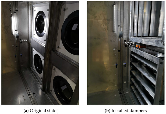
Figure 2.
Parallelly mounted fans within the AHU with and without the individual air dampers.
As Ostmann et al. [8] showed, representing the experimental data by dimensionless metrics allows a better prediction when applying polynomial models. The flow coefficient relates the average axial velocity to the circumferential velocity at the impeller diameter according to Equation (1) [15]. The circumferential velocity is calculated by the fan speed (in rev/s/s) and the impeller diameter using Equation (2).
The static-to-static pressure rise is measured across the supply air fans as shown in Figure 1. The pressure coefficient relates the static-to-static pressure rise to the dynamic pressure at the impeller exit according to Equation (3) [15].
To analyse the fan performance, the electric power consumption of each fan is measured individually. The total electric power consumption represents the sum of the electric power consumption of all active fans. The power coefficient relates the fan power to the product of the total fan casing area, circumferential velocity, and dynamic pressure at the impeller exit according to Equation (5) [15].
The static-to-static efficiency can be expressed by these three coefficients according to Equation (6), leading to the widely known definition of fan efficiency [15].
A summary of the relevant geometric parameters of the fan impeller and the assumption regarding the air state used for nondimensionalisation is given in Table 1.

Table 1.
Fan data and assumptions.
Due to physical and design limitations of the air handling unit, the fan system’s operation range is limited to the following:
- A total of 2000 m3/h 10,000 m3/h (limited by the volume flow measurement device).
- (design specification of the air handling unit).
- A total of (design specification of the fans).
By shutting off individual fans, various combinations of active fans are possible. This study focuses on the configurations of two active fans () and four active fans (). There are six possible combinations of how to select the active fans in the case of two fans. Figure 3 shows the experimentally captured performance maps for one, instead of all six, two-fan and the four-fan configuration according to Ostmann et al. [8]. The solid lines show the pressure rise, and the dashed lines represent the efficiency. Each speed line consists of eight operating points that are equally distributed over the volume flow range. From here on we will refer to an operating point as “sample” to be consistent throughout the article. A dataset is comprised of multiple samples. Our datasets consist of 240 samples for the two-fan configuration and 48 samples for the four-fan configuration. Given the respective data reduction level, we use the whole available dataset for training the polynomial model.
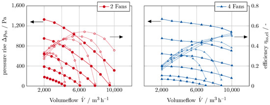
Figure 3.
Recorded performance maps of the investigated fan configurations acquired by Ostmann et al. [8]. For the two-fan configuration only a single combination is shown.
To assess the sensitivity of both models for less available data, we apply a two-stage reduction of the dataset. Therefore, the measured data are sorted randomly. In the next step, the number of samples is reduced by cutting the randomly sorted dataset from the lower end. In the first stage, the dataset is reduced by 25%, and in the second stage, it is further reduced to 50%. The same datasets are then used to fit the polynomial and machine learning models, respectively.
2.2. Polynomial Description
The polynomial model is described in detail by Ostmann et al. [8], but a short explanation is also given here. When representing fan performance data by their respective, dimensionless coefficients, the resulting performance maps are less curved. This allows for a more obvious derivation of polynomial functions to approximate fan performance [8]. Another advantage is the possibility of scaling the description to other fan diameters or fan speeds.
To approximate the pressure rise, the formulation according to Equation (7) is used. It produces good results for datasets with smaller flow coefficients, which is true for both investigated datasets. It can be reformulated to yield the pressure rise according to Equation (8) [8].
The power coefficient is approximated similarly to the pressure coefficient according to Equation (9). The efficiency is calculated according to Equation (10) using the relationship from Equation (6) and inserting the expressions for , , and . We use the approximated pressure-rise from Equation (8) to calculate the electric fan power consumption according to Equation (11).
The electric fan power is computed from the predicted pressure rise and efficiency by using the relation in Equation (6). In the above equations, the volume flow is expressed in m3/s and the fan speed is expressed in rev/s.
We compute the polynomial coefficients by solving the minimisation problem formulated in Equation (12). Here is the quantity that is to be approximated. We employ the non-linear implementation of a Generalised Reduced Gradient (GRG) solver as proposed by Lasdon et al. [16].
2.3. Machine Learning
In our machine learning approach, we employ the ADDMo tool as our primary resource [17]. ADDMo stands as an automated machine learning pipeline that seamlessly guides through various stages, starting from raw input data and proceeding through data refinement, model optimisation, evaluation, documentation, and visualization. ADDMo encompasses a range of advanced machine learning algorithms, including Artificial Neural Networks (ANN), Support Vector Regression (SVR), Gradient Tree Boosting (GB), Random Forest (RF), and the linear model Lasso. For a more comprehensive understanding of ADDMo, we direct readers to its original exposition in the referenced article [17].
Within the model optimisation phase of the pipeline, ADDMo leverages hyper-parameter optimisation through Bayesian optimisation for each machine learning algorithm. This optimisation process includes cross-validation to avoid overfitting. In our specific study, we opted for 300 iterations for the Bayesian optimisation and employed a five-fold cross-validation strategy.
The input features for each model calibration process are the fans’ speed and volume flow, while the targets are the fan power and total static pressure rise. We train separate machine learning models for each target variable and use case.
Upon conducting initial assessments, it becomes evident that SVR, as described by Vapnik [18], outperforms other machine learning algorithms for our specific task. SVR not only demonstrates remarkable accuracy but also exhibits strong interpolation capabilities within the input space, as well as reasonable extrapolation performance at the boundaries of the input space. SVR accomplishes this by mapping the input data to a higher-dimensional space, where it can effectively represent the data using linear functions or hyperplanes. Consequently, our analysis focuses on SVR, as implemented and described in LibSVM [19].
2.4. KPIs for Model Quality Evaluation
We define the mean relative error (MRE) and the absolute relative error (ARE) as quality metrics by introducing the auxiliary quantity , which represents either the pressure rise or the efficiency, according to Equations (13) and (14).
The reference values used for normalisation are and , respectively. A lower quality metric value indicates a lower error between the predicted and measured value and, therefore, a better model quality. To evaluate the quality, we compare the models’ predictions against the full available dataset instead of only the reduced data sets used to develop or train the models.
2.5. Performance Evaluation in the Scope of an Office Building
To compare the performance of the polynomial and SVR models, we define a simulation use case consisting of a simplified office building shown in Figure 4 that is supplied by an AHU with the fan configuration as used in the experimental investigations. The office building comprises nine zones ventilated by a central AHU. The AHU supplies air for up to 190 occupants with a required volume flow rate of per person with a demand-controlled ventilation strategy. We neglect the energy demand required for the extraction of the air out of the building to simplify the calculations. Each zone is modelled with a constant pressure loss coefficient representing a flow resistance that is the sum of the central duct system and a zone-specific resistance. The goal is to compute the AHU’s electric energy demand for building ventilation and use it to compare the performance of our models.
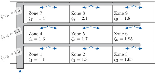
Figure 4.
Structure of the simplified office building.
We calculate the required pressure rise the AHU has to provide according to Equation (15) and the supply air volume flow according to Equation (16).
Here, the air density is kept constant at , and the AHU’s channel cross-section is simplified to . The model assumes a constant flow velocity in the whole duct system, leading to decreasing cross-sectional area when moving downstream the duct system. The AHU provides a basic supply regardless of occupancy of , which leads to . Since we assume a varying occupancy for each zone during daily operation, the required total volume flow varies as well. Furthermore, the unoccupied zones are not ventilated and, therefore, do not contribute to the required pressure rise. Depending on the occupied zones, we calculate the maximum required pressure rise to ventilate the zone with the most significant resistance. For example, assuming only zone 3 and zone 8 are occupied, the resulting flow resistance is calculated according to Equation (17).
We compute the electric energy demand over a whole year, consisting of 52 weeks, with a resolution of . During all weekends (Saturday and Sunday), the AHU supplies the minimum volume flow only. We develop five occupancy profiles assuming different occupancies of the zones with varying periods where the zones are occupied. Furthermore, we randomise the occurrence of the five profiles within each week to generate the occurring operating points of the AHU as shown in Figure 5a. The time history of the supply volume flow and the required pressure rise for one example week is shown in Figure 5b, with the respective occupancy profiles of the different zones shown in Figure 6.
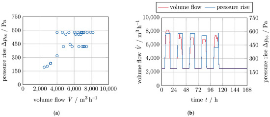
Figure 5.
Overview of the operating points based on the building demand. (a) Operating points occurring across the whole year. (b) Time history of one week with all five reference days.
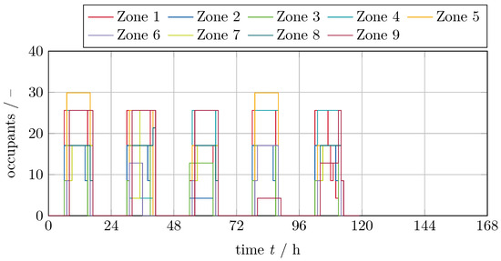
Figure 6.
Overview of the occupancy for all five reference days.
We compute the electric energy demand for every timestep by evaluating the developed models with the respective operating points according to the building demand. The models compute the pressure rise and the electric power according to Equations (18) and (19).
Since an operating point is defined by we determine the required fan speed to match the required pressure rise by evaluating the model from Equation (18) iteratively. By applying a Newton scheme, the fan speed is found within 10 iterations with a residual of the pressure rise below . Once the fan speed is determined, we compute the electric power demand and integrate it to the energy demand for the whole year according to Equation (20).
To evaluate the ability of our models to extrapolate, we increase the required volume flow rate to but keep all other assumptions such as , and the pressure loss coefficients constant. Consequently, the amount of supply air increases, which further increases the necessary pressure rise (see Equation (18)). This resembles the case where an increased amount of fresh air is required without the possibility of adapting the ventilation system, assuming the fans can provide the necessary power.
3. Results
The results are presented in the same fashion for both investigated configurations. To give an impression of the fitted models’ quality and shape, carpet plots are used. Each set consists of the pressure rise and the fan power, where the range is extended over the measured spectrum to demonstrate the extrapolation behaviour. The carpet plots are sampled with a regular grid. The volume flow is bounded by [0, 20,000] m3/h with a step size of , while the fan speed is bounded by [0, 4000] min−1 with a step size of 100 min−1. These limits enforce a rather extreme extrapolation towards higher volume flows by a factor of 2 and a moderate extrapolation towards higher fan speeds by a factor of about 1.43. For a better visualisation, values below zero are filtered out.
In addition to the carpet plot, the samples used to fit the respective model are represented by small dots  . Depending on whether the carpet plot is below or above the data point, the point is visible or partially hidden by the semi-transparent carpet plot. The used colourmaps are taken from Smith and van der Walt [20].
 . Depending on whether the carpet plot is below or above the data point, the point is visible or partially hidden by the semi-transparent carpet plot. The used colourmaps are taken from Smith and van der Walt [20].
3.1. Model Quality Metrics
The computed model quality metrics are summarised in Table 2 with the corresponding polynomial fit coefficients given in Table A1. For the two-fan configuration, more samples are available since in total six active fan arrangements are available, whereas the four-fan configuration consists of a single data set with 48 samples. This leads to clusters of comparable operating points scattered near each other [8]. Even for the most reduced dataset, there are enough samples available to cover all operating points.

Table 2.
Overview of quality metrics for the two-fan configuration.
Following the approach described by Ostmann et al. [8], the characteristic performance maps for the two-fan configuration and the four-fan configuration are shown in Figure 7. The polynomial fit is represented by the solid lines, while the underlying experimental data are indicated by the dashed lines. Regarding the two-fan configuration, the polynomial model represents the average of all these combinations. The different fan arrangements are close to each other and, therefore, allow this simplification. The four-fan configuration consists of only one data set, which is well captured by the polynomial prediction.
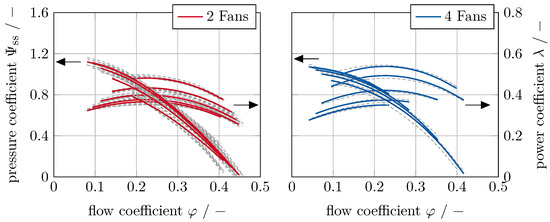
Figure 7.
Characteristic performance maps for the two-fan and four-fan configurations according to Ostmann et al. [8].
Regarding the two-fan configuration, the SVR prediction yields better quality metrics for all datasets, although the quality metrics are within the same magnitude (see Table 2). When reducing the dataset, the prediction of the pressure rise of the polynomial model improves slightly, presumably because of the reduced scatter at comparable operating points. The SVR prediction is negatively impacted by the reduced available data, although the effect is small compared with the overall quality. When the dataset is reduced, the fan power prediction is improved for all models, but the SVR model benefits more from the reduction than the polynomial model.
For the four-fan configuration, the computed model quality metrics are summarised in Table 3 with the corresponding polynomial fit coefficients given in Table A2. Due to the reduced scatter, the overall model quality is improved compared with the two-fan models. Our SVR model achieves better quality metrics than the polynomial prediction in nearly all aspects. However, the polynomial model yields a better MRE of the pressure rise for both reduced datasets. We observe an increase of the MRE of the pressure rise SVR prediction by a factor of nearly 3 when halving the training data. For the polynomial prediction, we achieve a slight decrease in the MRE when reducing the dataset.

Table 3.
Overview of quality metrics for the four-fan configuration.
3.2. Prediction of the Fan Performance Maps
In Figure 8, the carpet plots of the polynomial prediction of the two-fan configuration with full input data are shown. The carpet plots for both available data reduction levels are given in Figure A1. The prediction of the SVR model of the same configuration is shown in Figure 9, while the other data reduction levels are shown in Figure A2.
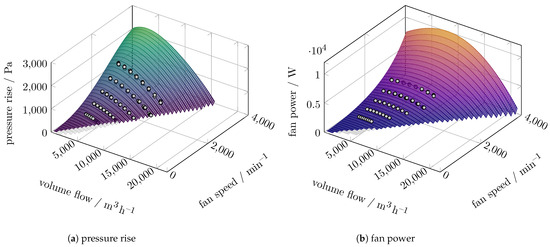
Figure 8.
Carpet plots for the pressure increase and power polynomial prediction of the two-fan configuration with 100% data.
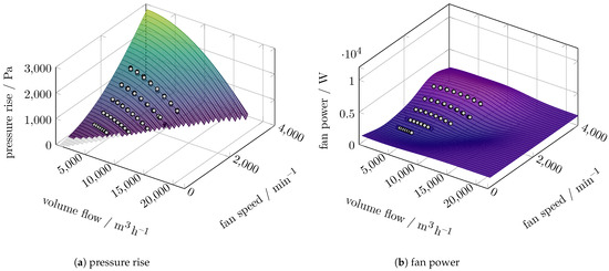
Figure 9.
Carpet plots of the SVR prediction for the pressure increase and power of the two-fan configuration with 100% data.
Both models can predict the pressure rise qualitatively well when extrapolating towards higher fan speeds or volume flows. The quality of the prediction within the extrapolation range is based on the theoretically expected dependency of the pressure rise on the fan speed (, see Equation (3)). Only the polynomial model can predict the fan power within the expected limits, as the fan power is not expected to decrease with increasing fan speed (, see Equation (5)). Although we do not explicitly show the efficiency (see Equation (6)), we investigate the representative operating point at (7500 m3/h, 4000 min−1) within the extrapolating range of both models. The polynomial models predict fan efficiencies in the range 37.7–40.8%. The SVR model underpredicts the fan power when leaving the area where measured data are available. This leads to overpredicted fan efficiencies above 100% at (7500 m3/h, 4000 min−1) for all data reduction levels.
Figure A2c showcases the impact of a reduction of the available data points. We observe that the general behaviour of both the polynomial and the SVR models does not change significantly. However, if the SVR model is trained with only 75% of the available data, it underpredicts the pressure rise towards higher fan speeds, leading to an unphysical local maximum near medium fan speeds.
The carpet plots of the four-fan configuration can be found in Figure A3 and Figure A4. For all four-fan configurations, both the polynomial and the SVR predict the pressure rise well, even in the extrapolation range. Only the utilisation of the dataset with 50% reduction leads to an unprediction in maximum pressure rise when applying the SVR model. The fan power is underpredicted for all SVR models, although in contrast to the two-fan configuration, they do not feature a decrease towards increasing fan speeds. Choosing (1500 m3/h, 4000 min−1) as the operating point in the extrapolation range, the fan efficiency is evaluated to 34.2–38.8% according to the polynomial prediction. At the same operating point, the SVR models predict the fan efficiency to 51.0–83.5% depending on the data reduction level.
3.3. Electric Energy Demand for the Reference Office Building
The resulting electric energy demand from applying the models to the reference office building is shown in Figure 10. For the two-fan configuration, the polynomial models predict a slightly higher energy demand of roughly 7480 MWh/a when compared with roughly 7370 MWh/a as predicted by the SVR models. While the energy demand predicted by the polynomial does not significantly change between the data reduction levels (), the demand predicted by the SVR model varies by roughly 1.8%. The two-fan configurations are all predicted to require a maximum fan speed of 2700 min−1 to satisfy the building demand, which is close to the edge of the measured domain.
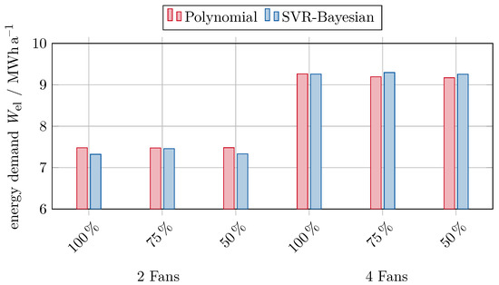
Figure 10.
Energy demand as predicted by all models for the reference office building with .
The four-fan configurations require roughly 24% more energy than their two-fan counterparts. The required maximum fan speed of roughly 2100 min−1 is lower than for the two-fan configurations since the load is spread between more fans and the operating point for each individual fan is shifted (see [8]). In the case of the four-fan configurations, the polynomial models are more sensitive to a reduction of the available data, as the results vary by close to 1%. In contrast, the SVR results only differ by about 0.4%.
Overall, the results are very close together within the respective fan configurations, as the building demand is well within the domain captured by the datasets used for fitting or training the models.
When increasing the person-specific volume flow rate to , the two-fan configuration is not able to deliver the necessary volume flow rate and pressure rise anymore. Therefore, only the four-fan configuration is evaluated, and the respective results for the energy demand are shown in Figure 11.
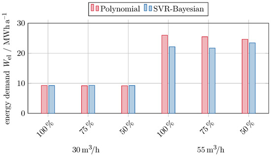
Figure 11.
Comparison of the energy demand as predicted by the four-fan models with increased required volume flow rate per person.
When increasing the overall required volume flow rate, the energy demand increases by more than 140% to roughly 22,400 MWh/a or 25,300 MWh/a for the SVR or polynomial prediction, respectively. Since the maximum required fan speed also increases to roughly 3300 min−1, all models are evaluated in areas where they are extrapolating the underlying data used for fitting or training. When we evaluate the SVR prediction based on the dataset reduced by 50% we observe a maximum fan speed of 3800 min−1, because the pressure rise is generally underpredicted (see Figure A4e) when compared with the other two data reduction levels (see Figure A4a,c).
The deviation between the data reduction levels does increase as well. While the energy demand predicted by the polynomial models decreases by 5.5% with decreasing data availability, the values predicted by the SVR models vary by 8% with no clear trend.
4. Discussion
All developed models yield consistent results for the electric energy demand if the occurring operating points for which the models are evaluated lie within the domain where samples are available for fitting and training of the models. All models benefit from including the low and high fan speed samples in particular. This information is crucial for the good performance of our models, as it is required for the adaptation of the fan speed-related behaviour. The samples at medium fan speeds are less important, although a good distribution across different fan speeds should be maintained. The polynomial model seems more capable of producing consistent results when one operating point consists of a cluster of multiple samples, as for the two-fan configuration. In these configurations, at least one sample is available for each operating point, even when reducing the input data set by 50%. If an operating point is entirely omitted by reducing the input data, as for the four-fan configuration, the SVR yields more consistent results featuring less scatter between the data reduction levels.
When extending the operating point range towards higher loads (increasing volume flow rate and pressure rise) and therefore leaving the area where training samples are available, the computed electric energy demands deviate apart. From theory, it is known that the aerodynamic power of a fan scales with the fan speed (, see Equation (5)). The SVR models fail to give a good prediction of the fan power in this regard, which is apparent when considering the presented predicted fan power within the extrapolation area. When evaluating the two-fan SVR prediction, the fan power features local maxima near the edge of the experimentally captured domain with decreasing fan power when stepping further into the extrapolating range. This leads to unphysical results for the two-fan configuration. In the case of the four-fan SVR prediction, the general trend is captured by the model, but still, the cubic dependency is not met. Therefore, the predicted efficiencies are too high to be within the typical range of about 50–65%. This renders the SVR models unfeasible to be utilised outside the domain captured experimentally.
The deviation of the computed electric energy demand is below 2% when investigating the lower specific volume flow rate. We deem this to be a good result showcasing the validity of the models. As soon as we increase the specific volume flow rate, the number of operating points residing within the extrapolation range is also increased. This leads to deviations of up to 13% between the two modelling approaches. As we already discussed, the polynomial model tends to better fit the expected cubic dependency on the fan speed. Therefore, we hold the polynomial prediction to be more trustworthy than the SVR prediction.
5. Conclusions
This paper presents polynomial and SVR models to predict fan performance. In the scope of parallelly operated fans, we used two sets of possible fan arrangements. We fitted and trained the models based on experimental data available in various data densities. We applied the models to a simplified office building to rate the quality of their predictions for a wide range of operating points both inside and outside of the experimentally captured domain.
When evaluating the models inside the experimentally captured domain, both approaches yield results that are in close agreement with each other. As soon as the evaluation is conducted on operating points outside the experimentally captured domain, the deviation between the results increases the further away the operating points are from the original data set. This is mainly due to the SVR failing to properly predict the fan power towards higher fan speeds. While the polynomial models compute fan efficiencies within a plausible range, the SVR yields unphysically high efficiencies. Extrapolation is a difficult task for any statistical model. However, in our investigated case, polynomial models seem more robust for that task than the here-tested SVR.
In upcoming studies, a physics-informed approach could be investigated to improve the extrapolation capability of the models. The physical information would need to be extremely simple and well generalisable to maintain the advantage of fast and easy modelling through machine learning algorithms. Such an explicit analysis of the extrapolation domain would also require an extension of the experimentally captured domain towards higher fan speed to generate a ground truth. Additionally, further demand scenarios could be analysed.
Author Contributions
Conceptualization, P.O. and M.R.; methodology, P.O. and M.R.; validation, P.O., M.R. and M.K.; formal analysis, P.O. and M.R.; investigation, P.O.; resources, P.O.; data curation, P.O. and M.R.; writing—original draft preparation, P.O. and M.R.; writing—review and editing, P.O., M.R. and M.K.; visualization, P.O.; supervision, M.K. and D.M.; project administration, M.K. and D.M.; funding acquisition, D.M. All authors have read and agreed to the published version of the manuscript.
Funding
This research was funded by BMWK (Federal Ministry for Economic Affairs and Climate Action), grant number 03ET1606B.
Institutional Review Board Statement
Not applicable.
Informed Consent Statement
Not applicable.
Data Availability Statement
Data are contained within the article.
Conflicts of Interest
The authors declare no conflicts of interest. The funders had no role in the design of the study; in the collection, analyses, or interpretation of data; in the writing of the manuscript; or in the decision to publish the results.
Abbreviations
The following abbreviations are used in this manuscript:
| AHU | Air handling unit |
| ETA | Extract air |
| EXH | Exhaust air |
| ODA | Outdoor air |
| SUP | Supply air |
| SVR | Support vector regression |
Appendix A
Appendix A.1. Polynomial Coefficients for the Developed Models

Table A1.
Coefficients of the two-fan polynomial models.
Table A1.
Coefficients of the two-fan polynomial models.
| Dataset | / | / | ||||||
|---|---|---|---|---|---|---|---|---|
| 0 | 1 | 2 | 3 | 4 | 0 | 1 | 2 | |
| 100% | −1.79 | −3.67 × 101 | 1.99 × 10³ | −2.48 × 10⁴ | 1.41 × 10⁵ | −1.09 × 10⁻¹ | −9.52 × 10⁻³ | 1.11 × 10⁻⁴ |
| 1.70 × 10⁻¹ | 3.31 | −2.94 × 101 | −5.14 × 10² | 2.33 × 10³ | 2.48 × 10⁻¹ | 4.87 × 10⁻³ | 5.02 × 10⁻⁵ | |
| 75% | 7.37 × 10⁻¹ | 1.52 × 101 | −7.99 × 10² | 9.53 × 10³ | −5.27 × 10⁴ | 2.94 × 10⁻¹ | 2.09 × 10⁻² | −2.32 × 10⁻⁴ |
| 3.57 × 10⁻² | 8.10 × 10⁻¹ | −1.04 × 101 | −3.88 × 101 | 2.11 × 101 | 1.19 | −2.48 × 10⁻² | 2.66 × 10⁻⁴ | |
| 50% | 9.27 × 10⁻¹ | 4.87 | −3.34 × 10² | 2.23 × 10² | 8.35 × 10³ | 2.26 × 10⁻¹ | 2.06 × 10⁻² | −2.41 × 10⁻⁴ |
| 3.26 × 10⁻² | 7.74 × 10⁻¹ | −1.01 × 101 | −3.50 × 101 | 6.16 × 101 | 1.25 | −2.45 × 10⁻² | 2.53 × 10⁻⁴ | |

Table A2.
Coefficients of the four-fan polynomial models.
Table A2.
Coefficients of the four-fan polynomial models.
| Dataset | / | / | ||||||
|---|---|---|---|---|---|---|---|---|
| 0 | 1 | 2 | 3 | 4 | 0 | 1 | 2 | |
| 100% | 9.12 × 10⁻¹ | −1.42 × 10⁻¹ | −3.26 × 101 | −1.65 × 10² | −3.34 × 10² | 4.50 × 10⁻¹ | 9.51 × 10⁻³ | −1.06 × 10⁻⁴ |
| 1.56 × 10⁻¹ | 2.10 | −1.47 × 101 | −1.40 × 101 | 2.22 × 101 | 6.19 × 10⁻¹ | −1.70 × 10⁻² | 1.96 × 10⁻⁴ | |
| 75% | 9.23 × 10⁻¹ | −7.18 × 10⁻¹ | −2.08 × 101 | −2.17 × 10² | −5.29 × 10² | 4.62 × 10⁻¹ | 8.63 × 10⁻³ | −9.34 × 10⁻⁵ |
| 1.58 × 10⁻¹ | 2.19 | −1.54 × 101 | −1.20 × 101 | 3.33 × 101 | 5.87 × 10⁻¹ | −1.57 × 10⁻² | 1.80 × 10⁻⁴ | |
| 50% | 1.21 | −3.73 × 10⁻¹ | −3.65 × 101 | −2.55 × 10² | −4.88 × 10² | 3.68 × 10⁻¹ | 5.26 × 10⁻³ | −5.20 × 10⁻⁵ |
| 1.58 × 10⁻¹ | 1.93 | −1.22 × 101 | −2.19 × 101 | −1.20 × 101 | 5.97 × 10⁻¹ | −1.57 × 10⁻² | 1.77 × 10⁻⁴ | |
Appendix A.2. Predicted Data for Two Fan Configuration
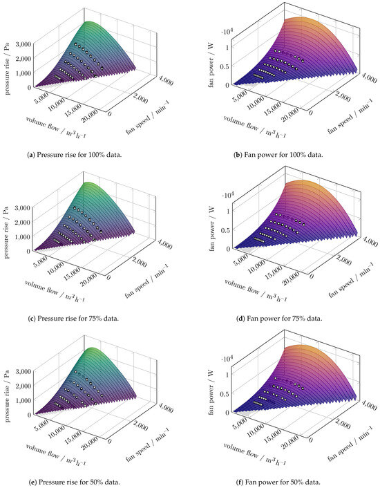
Figure A1.
Carpet plots for the pressure increase and power polynomial prediction of the two-fan configuration.
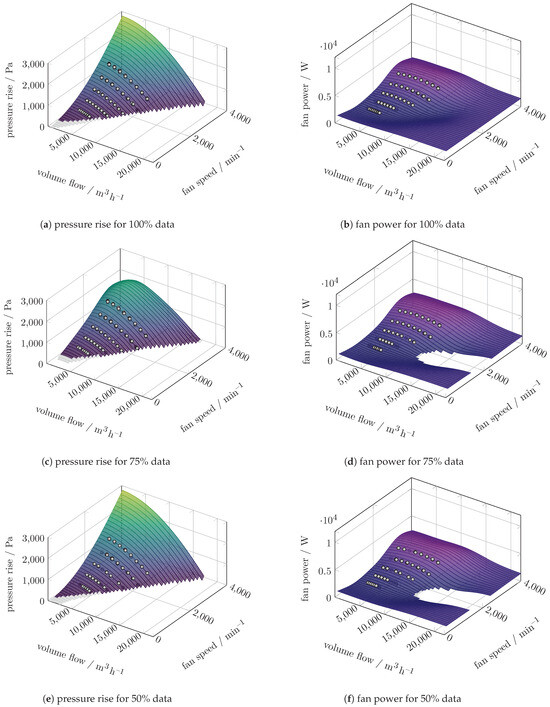
Figure A2.
Carpet plots for the pressure increase and power SVR prediction of the two fans configuration.
Appendix A.3. Predicted Data for Four Fan Configuration
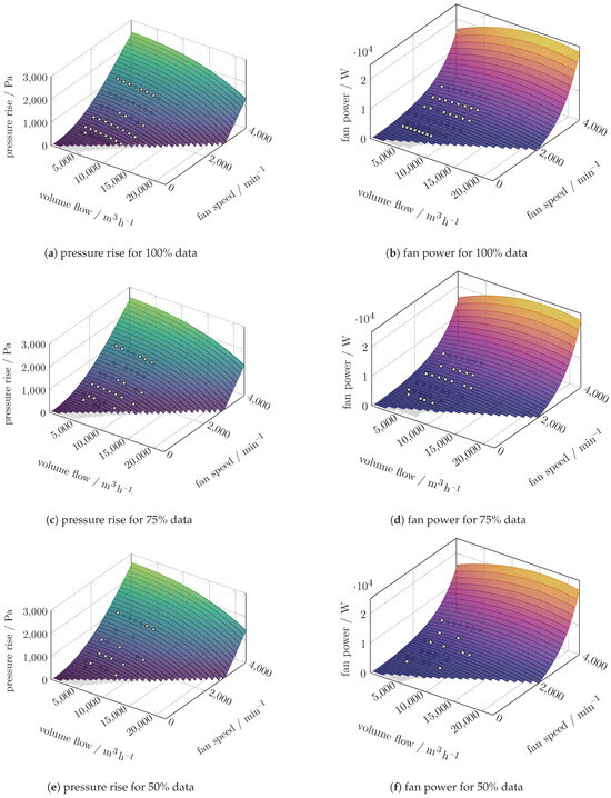
Figure A3.
Carpet plots for the pressure increase and power polynomial prediction of the four-fan configuration.
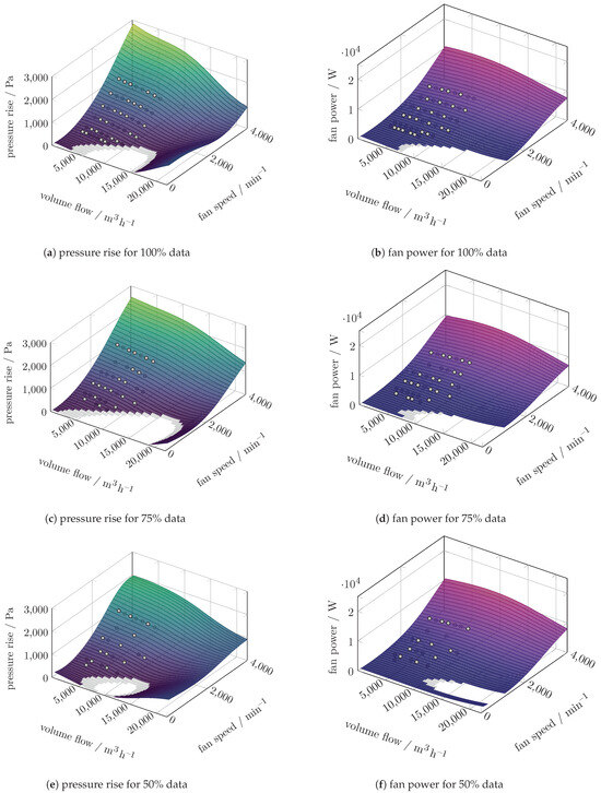
Figure A4.
Carpet plots for the pressure increase and power SVR prediction of the four fans configuration.
References
- Klepeis, N.E.; Nelson, W.C.; Ott, W.R.; Robinson, J.P.; Tsang, A.M.; Switzer, P.; Behar, J.V.; Hern, S.C.; Engelmann, W.H. The National Human Activity Pattern Survey (NHAPS): A Resource for Assessing Exposure to Environmental Pollutants. J. Expo. Anal. Environ. Epidemiol. 2001, 11, 231–252. [Google Scholar] [CrossRef] [PubMed]
- Diffey, B.L. An Overview Analysis of the Time People Spend Outdoors. Br. J. Dermatol. 2011, 164, 848–854. [Google Scholar] [CrossRef] [PubMed]
- Schiller, H.; Mai, R.; Händel, C. Chancen der Energetischen Inspektion für Gesetzgeber, Anlagenbetreiber und die Branche—Abschlussbericht zum Forschungsvorhaben; Technical Report; Forschungsinitiative Zukunft Bau: Salzburg, Austria, 2014. [Google Scholar]
- Jones, D.A.; Eckert, C.M. Empowering Decision Makers to Avoid the Oversizing of Building Service Systems. In Proceedings of the 22nd International Conference on Engineering Design (ICED19), Delft, The Netherlands, 5–8 August 2019; pp. 1135–1144. [Google Scholar] [CrossRef]
- Merema, B.; Delwati, M.D.; Sourbron, M.; Breesch, H. Demand Controlled Ventilation (DCV) in School and Office Buildings: Lessons Learnt from Case Studies. Energy Build. 2018, 172, 349–360. [Google Scholar] [CrossRef]
- Rätz, M.; Kalliomäki, P.; Mathis, P.; Koskela, H.; Müller, D. Analyzing the Energy-Saving Potential of Demand-Controlled Ventilation in Hospitals via Dynamic Building Simulations. In Proceedings of the 16th International Conference on Indoor Air Quality and Climate (Indoor Air 2020), Seoul, Republic of Korea, 20–24 July 2020. [Google Scholar]
- Breuer, J.; Müller, T.M.; Pelz, P.F. How to Save Energy in Ventilation Systems through Distributed Fans. In Proceedings of the Fan 2022—International Conference on Fan Noise, Aerodynamics, Applications and Systems, Senlis, France, 27–29 June 2022. [Google Scholar] [CrossRef]
- Ostmann, P.; Kremer, M.; Müller, D. Efficiency Increase of Air Handling Units by Parallely Operated Fans. In Proceedings of the Ventilation 2022: 13th International Industrial Ventilation Conference for Contaminant Control, Toronto, ON, Canada, 15–18 August 2021; pp. 298–306. [Google Scholar] [CrossRef]
- Conrad, D.; Mayer, J.; Reichert, E. Optimization, Control and Design of Arbitrarily Shaped Fan Arrays. In Proceedings of the Fan 2022—International Conference on Fan Noise, Aerodynamics, Applications and Systems, Senlis, France, 27–29 June 2022. [Google Scholar] [CrossRef]
- Maier, L.; Jansen, D.; Wüllhorst, F.; Kremer, M.; Kümpel, A.; Blacha, T.; Müller, D. AixLib: An Open-Source Modelica Library for Compound Building Energy Systems from Component to District Level with Automated Quality Management. J. Build. Perform. Simul. 2023, 17, 196–219. [Google Scholar] [CrossRef]
- Wetter, M.; van Treeck, C.; Helsen, L.; Maccarini, A.; Saelens, D.; Robinson, D.; Schweiger, G. IBPSA Project 1: BIM/GIS and Modelica Framework for Building and Community Energy System Design and Operation—Ongoing Developments, Lessons Learned and Challenges. IOP Conf. Ser. Earth Environ. Sci. 2019, 323, 012114. [Google Scholar] [CrossRef]
- Stein, J.; Hydemann, M.M. Development and Testing of the Characteristic Curve Fan Model. ASHRAE Trans. 2004, 110, 347–356. [Google Scholar]
- Singh, M.; Jradi, M.; Shaker, H.R. Monitoring and Evaluation of Building Ventilation System Fans Operation Using Performance Curves. Energy Built Environ. 2020, 1, 307–318. [Google Scholar] [CrossRef]
- Fu, H.; Blum, D.; Wetter, M. Fan and Pump Efficiency in Modelica Based on the Euler Number. In Proceedings of the American Modelica Conference 2022, Dallas, TX, USA, 26–28 October 2022. [Google Scholar] [CrossRef]
- Carolus, T. Ventilatoren: Aerodynamischer Entwurf, Schallvorhersage, Konstruktion, 3rd ed.; Vieweg+Teubner Verlag Imprint: Wiesbaden, Germany, 2013. [Google Scholar]
- Lasdon, L.; Fox, R.; Ratner, M. Nonlinear Optimization Using the Generalized Reduced Gradient Method. Rev. Franç. d’Autom. Inform. Rech. Opérat. Série Verte 1973, 8, 63. [Google Scholar] [CrossRef]
- Rätz, M.; Javadi, A.P.; Baranski, M.; Finkbeiner, K.; Müller, D. Automated Data-Driven Modeling of Building Energy Systems via Machine Learning Algorithms. Energy Build. 2019, 202, 109384. [Google Scholar] [CrossRef]
- Vapnik, V.N. Statistical Learning Theory; A Wiley-Interscience Publication; Wiley: New York, NY, USA; Weinheim, Germany, 1998. [Google Scholar]
- Chang, C.C.; Lin, C.J. LIBSVM: A Library for Support Vector Machines. ACM Trans. Intell. Syst. Technol. 2011, 2, 27. [Google Scholar] [CrossRef]
- Smith, N.; van der Walt, S. A Better Default Colormap for Matplotlib. In Proceedings of the SciPy2015—Scientific Computing with Python, Austin, TX, USA, 6–12 July 2015; Enthought Inc.: Austin, TX, USA, 2015. [Google Scholar]
Disclaimer/Publisher’s Note: The statements, opinions and data contained in all publications are solely those of the individual author(s) and contributor(s) and not of MDPI and/or the editor(s). MDPI and/or the editor(s) disclaim responsibility for any injury to people or property resulting from any ideas, methods, instructions or products referred to in the content. |
© 2024 by the authors. Published by MDPI on behalf of the EUROTURBO. Licensee MDPI, Basel, Switzerland. This article is an open access article distributed under the terms and conditions of the Creative Commons Attribution (CC BY-NC-ND) license (https://creativecommons.org/licenses/by-nc-nd/4.0/).