Predictive Modeling of NOx Emissions from Lean Direct Injection of Hydrogen and Hydrogen/Natural Gas Blends Using Flame Imaging and Machine Learning

Abstract

This research paper explores the use of machine learning to relate images of flame structure and luminosity to measured NOx emissions. Images of reactions produced by 16 aero-engine derived injectors for a ground-based turbine operated on a range of fuel compositions, air pressure drops, preheat temperatures and adiabatic flame temperatures were captured and postprocessed. The experimental investigations were conducted under atmospheric conditions, capturing CO, NO and NOx emissions data and OH* chemiluminescence images from 27 test conditions. The injector geometry and test conditions were based on a statistically designed test plan. These results were first analyzed using the traditional analysis approach of analysis of variance (ANOVA). The statistically based test plan yielded 432 data points, leading to a correlation for NOx emissions as a function of injector geometry, test conditions and imaging responses, with 70.2% accuracy. As an alternative approach to predicting emissions using imaging diagnostics as well as injector geometry and test conditions, a random forest machine learning algorithm was also applied to the data and was able to achieve an accuracy of 82.6%. This study offers insights into the factors influencing emissions in ground-based turbines while emphasizing the potential of machine learning algorithms in constructing predictive models for complex systems.

1. Introduction

Combustion involves complex non-linear physical and chemical processes both on time and space scales. However, because of its wide use of energy, it is crucial to study its efficiency associated with the reduction in pollutant emissions. An extensive set of information has been established in the literature using the traditional approach of performing experimental studies, building combustion models to help explain the phenomena observed, and using these results to evolve designs for improved performance. It is likely that the data available could be further processed via machine learning techniques to gain further insight into the improvement of performance. One of the main goals of machine learning is to optimize predictive models; therefore, researchers have been using these algorithms in the field of combustion. Machine learning algorithms have a variety of applications, from chemical kinetics calculation acceleration to model uncertainty quantification and research of unknown reaction pathways [1]. However, limitations and challenges remain, typically related to the lack of generalizability and interpretability of models designed for specific applications, as well as the preprocessing of the data requirement.

Seeking carbon neutralization of gas turbines, hydrogen has an increasing role as an alternative fuel. Apart from the challenges inferred by its higher flame speeds compared to traditional natural gas fuels (flashback, autoignition and instabilities [2]), some of the literature has reported higher NOx emissions [3], but it has also been proven that lean premixed systems could reduce such pollutants [4]. Hence, to facilitate hydrogen’s optimal integration into the market, further research must be conducted. Historically, NOx emissions have been quantified using extractive sampling and gas analyzers, systems that are generally complex and expensive. For combustion system design direction, time-efficient alternatives are of great interest to speed up the process. Of course, computational fluid dynamics (CFD) can assist in the process by generating results relatively quickly. However, the analysis of results from CFD is also critical to consider in terms of providing guidance on design optimization. This guidance could be improved using artificial intelligence techniques. In the present effort, the potential of using artificial intelligence applications on relatively time-efficient data obtained via flame images is explored. Golgiyaz et al. [5] established a relationship between coal flame visible images and NOx emissions, with an accuracy of 95.22%, feeding the AI (artificial intelligence) model with 3780 measurements. Qin et al. [6] demonstrated a NOx predictive deep learning model with an error lower than 3% for oxy-biomass combustions based on two-color pyrometry for computing the flame temperature. The correlation between flame temperature and NOx is well established [7], so such a model has a physical basis.

A relationship between NOx emissions and OH* flame radicals has also been established by several authors. Flame radicals are generally active within the flame reaction, so they are markers of the heat release. Liu et al. [8] showed a linear increasing trend of NOx emissions in a lean premixed dual-swirl flame as a function of the OH* chemiluminescence. The authors of the current effort [9] also confirmed the linear regression of NOx with OH*. Therefore, the prediction of NOx emissions through flame radicals presents an avenue worthy of future research lines, as shown by Li et al. [10].

The objective of the current work is to construct a predictive model for NOx emissions from lean direct injection of hydrogen and hydrogen/natural gas blends, using flame imaging diagnostics and statistical or machine learning models. In this way, the current effort aims to consolidate and build upon previous findings relating NOx prediction with OH* chemiluminescence. The complexity added to the present study lies in the integration of multiple factors that may affect the NOx emissions. Not only are the combustion conditions varied, but so is the injector geometry. Hence, a versatile model is sought that is able to handle diverse variables to predict emissions based on the imaging characterization.

To help provide context for the current machine learning (ML) approach, more traditional analysis methods (in this case, analysis of variance) are used to complement and compare with ML analysis. A comparison of the two approaches is implemented since both are distinct in the way they establish the resulting model. The statistical method (e.g., ANOVA) is typically “top-down”, meaning that the model is assumed and its parameters are estimated, thus pre-assuming the type of relationship between the input variables and the output response. Statistical models typically consider linear relationships between variables (linear regression), whereas polynomial regressions can include non-linearities but might not capture the complexity of the relationships. On the other hand, machine learning algorithms are “bottom-up”, where no model is pre-assumed, but the algorithm develops it to predict the response [11], and so the non-linear patterns are aggregated. The latter can handle larger data sets, and since they are data-driven, the accuracy is not limited by the user choosing the relationship. However, the drawback of machine learning algorithms could be the interpretability of the resulting model and, therefore, the importance of performing such a comparison.

Despite the aforementioned disadvantages of machine learning methods, there is still some work to be done to exploit its potential when dealing with emissions prediction with flame diagnostics. As presented in [12], flame monitoring is dependent on the burner, so techniques of automatic recognition might be used to extract characteristic features and solve image classification problems, as well as the strong capabilities of machine learning algorithms. Different authors have already presented their work on NOx prediction by means of artificial intelligence algorithms, such as Gluĉina et al. [13]. Authors like Xinli Li et al. [10] and Golgiyaz et al. [5] used flame image characterization as an additional input of the model.

2. Materials and Methods

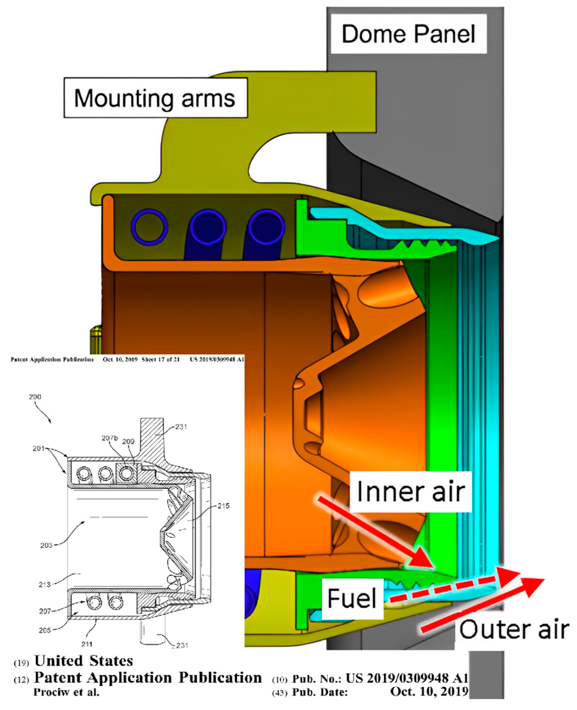
As discussed in [14], the experimental testing was conducted on a set of 16 gas-fueled injectors that were derived from liquid-fueled aero-engine injectors [15]. (For more details on the liquid injectors from which these were derived, please consult the United States Patent Application Publication number: US 2019/0309948 Al.) Thirteen of these were designed according to a statistical three-level Box–Behnken design [16], and three extra configurations were built to validate any model developed. The hardware developed resulted in a design space with varying air split (i.e., the percentage of air bypassing the air injection ports—“outer air” in Figure 1—over the total “inner air” and “outer air”), fuel swirl (i.e., the inclination with respect to the streamwise direction of the fuel injection ports), and air swirl (i.e., the inclination with respect to the streamwise direction of the air injection ports). The geometric parameters are illustrated in Figure 1 and Figure 2. The values for these three parameters were normalized from −1 to 1 for the current work, as the actual values used are proprietary.

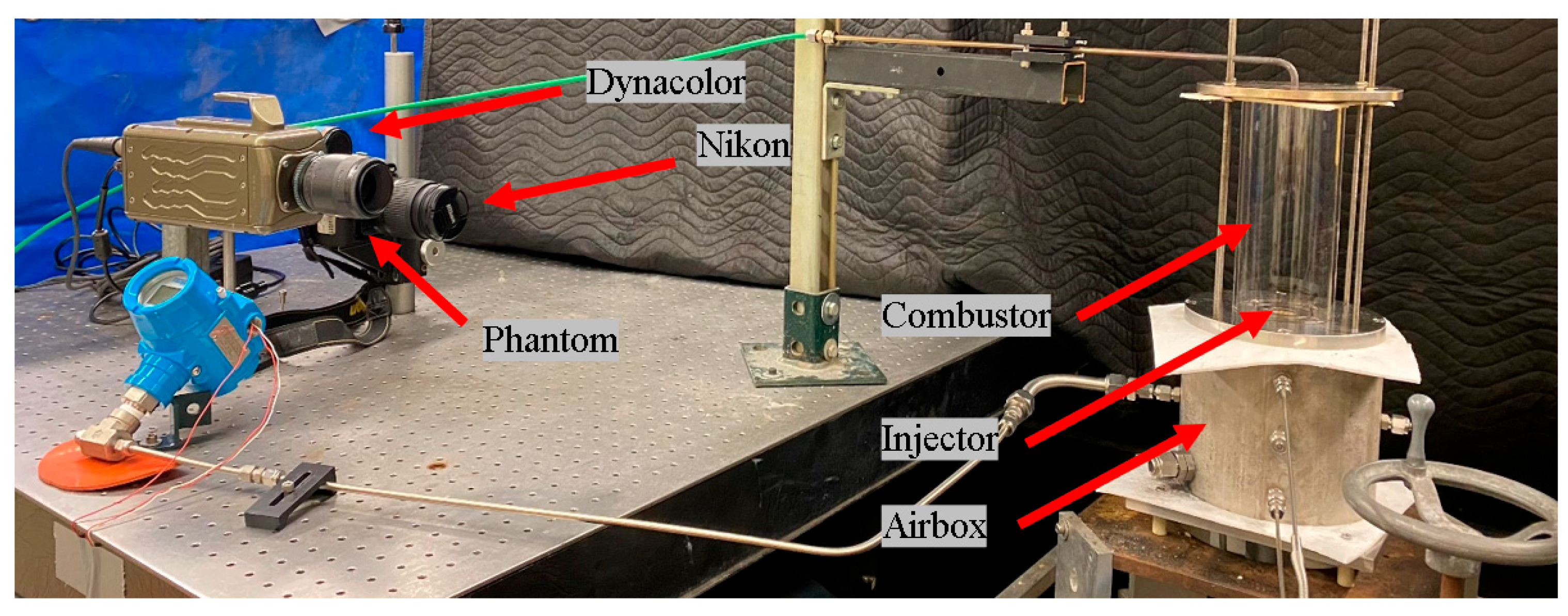
As shown in Figure 3, the injector was mounted inside an airbox (152.4 mm long, 146.3 mm inner diameter) and injected into a quartz tube (200 mm long, 80 mm inner diameter) used as a combustor liner. The injector was fed by the fuel line coming from the hydrogen and natural gas mass flow controllers, and the airbox was fed with air coming from the electric preheater. Each injector was tested under the same flow conditions, resulting from a three-level Box–Behnken design with four factors and three repeat points [9]: pressure drop of the air flow across the airbox (ranging from 2% to 6%), preheat temperature of the air flow (ranging from 465 K to 675 K), fuel composition (ranging from 0% hydrogen to 100% hydrogen, which is the mid-point of a 50% blend in the volume of both hydrogen and natural gas), and adiabatic flame temperature (ranging from 1500 K to 1850 K). This resulted in a 27-point matrix for each of the 16 injectors, so a total of 432 data points. It is noted that with this approach, each air pressure drop resulted in a difference in overall residence time. However, as shown in [9], the NOx emissions measured were not strongly influenced by residence time: pressure drop was insignificant to the model describing the NOx emissions.

2.1. Data Collection

For each condition, emissions were measured with a Horiba PG 350 (Horiba, Ltd.—Kyoto, Japan) gas analyzer: a 30 s moving average sample was collected at the center of the exhaust exit plate, pulled at a rate of 0.4 L/min. The sample was dried before being read by the analyzer, and the following measurements were recorded: percentages of O₂ and CO₂ and parts per million by volume dry corrected at 15% O₂ of CO, NO and NOx. Then, the latter data in ppmvd were converted into an ng/J basis using EPA Method 19, as reported in [9].

Additionally, two imaging approaches were operated for each test point simultaneously, as shown in Figure 3. A monochrome Dynacolor FB-N9-U (Dynacolor, Inc.–Taipei, Taiwan) was used to record the OH* chemiluminescence, keeping its exposure time constant at 999,900 μs and a digital gain of 6 dB, and the rest of settings at their default values as they were not observed to be critical for the recordings; a single frame was extracted from each recording. A visible-spectrum snapshot was taken with a Nikon D90 (Nikon Corporation—Tokyo, Japan) for each configuration, setting the manual mode to 2.5 shutter speed and F4 aperture.

2.2. Imaging Features Extraction

The main imaging features were extracted from the UV-spectrum recordings based on the direct correlation between the OH* and the flame front [18]. Each image was postprocessed with Matlab R2023b. First, Otsu’s method [19] was applied to determine the brightness intensity threshold from which pixels were considered as part of the flame. With the threshold defined, the monochromatic picture was binarized into flame and background segments so the flame contour could be extracted. A kernel neighbor averaging strategy was finally applied to overcome the influence of minor sources of random noise [20].

The flame area was quantified as the number of pixels from the binarized image, converted into area units with a known conversion factor based on the combustor’s outer diameter. Three main locations were then quantified: the top point of the flame, defining the flame length with respect to the injector outlet, and the points furthest to the left and right, defining the flame width. The last two points were also characterized by their height and horizontal location with respect to the injector base and center, respectively.

The OH* spectrum is typically characterized by its intensity or average grey level, as performed in [10]. As Liu et al. [8] concluded experimentally, there is a linear relationship between NOx emissions and OH* intensity (results corroborated by the authors’ team in [9]), so therefore it is an essential feature to be computed. For this study, the OH* intensity was mapped by its average value throughout the flame and its maximum value. The maximum value is used to define the heat release area: in this study, it was considered as the portion of the flame area with pixel intensities over 90% of the maximum brightness. This subsection was linked to the region where the majority of the heat release occurs [18], and it was characterized by its center of gravity (or geometric center) and its leading edge (the height of its bottom) with respect to the injector base. The location of the center of gravity was also quantified relative to the radial direction (see Figure 4 for a visual representation of the responses on a sample image). 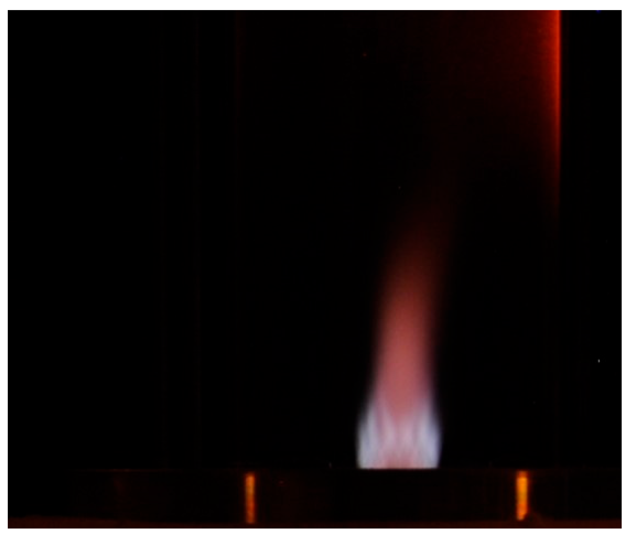The heat release area and its three characteristic distances were used by the authors in [9] to explain the increased emissions with lower mixing time (bigger region and closer to the injector). For context, Figure 5 shows the visible spectrum of this flame condition: 2% pressure drop, 650 K preheat temperature, 100% hydrogen, 1675 K adiabatic flame temperature.

2.3. Uncertainty

To contextualize the accuracy of the resulting algorithms, the uncertainty of the test result is needed. As summarized in [9], the cumulative uncertainty of the flow metering elements and the PG 350 gas analyzer yielded an average uncertainty of 11.1% in the NOx measurements. The uncertainty is based on the complete reaction of either methane, hydrogen, or a 50% blend in volume with air at the known flow rates of reactants (oxidizer and fuel). The expected values for O₂ and/or CO₂ from the combustion calculation were then compared to the measured values by the analyzer, and the difference was noted. The accuracy of each element in the setup was taken into account to draw the worst-case scenario from the computed emissions prior to the comparison with the measured values.

3. Results

Of the resulting 432 experimental measurements (27-point matrix for each of the 16 injectors), 34 were removed from the data set because of high CO levels that were recorded (in this case, taken as being levels above 500 ppmvd). These cases involved incomplete combustion and, therefore, resulted in a reduction in the total image intensity. In the current effort, as a first step, analysis without the possible bias associated with incomplete combustion was carried out. This is an admitted weakness in the use of imaging results because a priori knowledge of the combustion efficiency may not be known. In some systems, the O₂ measurement may be a routine measurement (e.g., in water heaters or boilers with O₂ trim capability), in which case some information may be available. Likewise, if CFD is used to generate results, more information about the overall combustion process will be available. But, in the case of imaging results in the present effort, cases with near 100% combustion efficiency were initially used. As a result, a total of 398 data points were used to construct the NOx predictive models based on the OH* images using the factors studied (injector geometry and combustion flow conditions). The following two approaches were taken: (1) a multivariate statistical analysis of variance (ANOVA) and (2) a machine learning algorithm. The former comes from the Box–Behnken testing design that was adopted, a model to map the design space. On the other hand, the machine learning algorithm allows the incorporation of additional non-linearities to the analysis, which has the potential to improve the accuracy of the data-driven model [11].

Both approaches are based on the same set of factors or features to obtain NOx emissions as the response: the three parameters of the injector geometry (air split, fuel swirl, air swirl), the four combustion conditions (pressure drop, preheat temperature, fuel composition, adiabatic flame temperature), and 13 responses from the OH* chemiluminescence recordings (flame height and width, horizontal and vertical location of the points furthest to the right and to the left, average and maximum brightness, flame and heat release areas, vertical and horizontal location of the center of gravity of the heat release area, and height of the leading edge of this area). The experimental measurements recorded an average NOx of 11.11 ng/J, with a standard deviation of 5.45 ng/J.

3.1. Statistical Model (ANOVA)

With the statistical design of the test matrix already constructed using the software Design Expert 13, the data set was imported and analyzed. The factors, or factor interactions, were taken as significant to the model when yielding p-values < 0.05. Terms up to the third order were considered. Because of the wide range of NOx values measured, the Box–Cox analysis indicated that a square root transform should be applied to the data to allow a third-order model to adequately represent the measured results. With these constraints, the ANOVA presented a standard deviation of 0.10, a coefficient of variance of 3.12%, R² = 0.9894, adjusted R² = 0.9827, predicted R² = 0.9660, and adequate precision of 68.73. The predicted and adjusted R² values were within reasonable agreement (difference less than 0.2), and the adequate precision showed an adequate signal-to-noise ratio.

The ANOVA showed that the five most significant factors based on their corresponding statistical F-values were the air split and air swirl interaction (F-value of 119.87), quadratic term of air split (F-value of 103.83), air split and air swirl interaction with a quadratic component of air swirl (F-value of 70.41), quadratic term of pressure drop (F-value of 64.65), and interaction between air split, fuel swirl and adiabatic flame temperature (F-value of 36.04). In a regression analysis, a large F-value suggests a significant improvement in explaining the variability of the dependent variable (NOx emissions, in this case) compared to a model with no predictors and, therefore, quantifies how important the term is to the overall model.

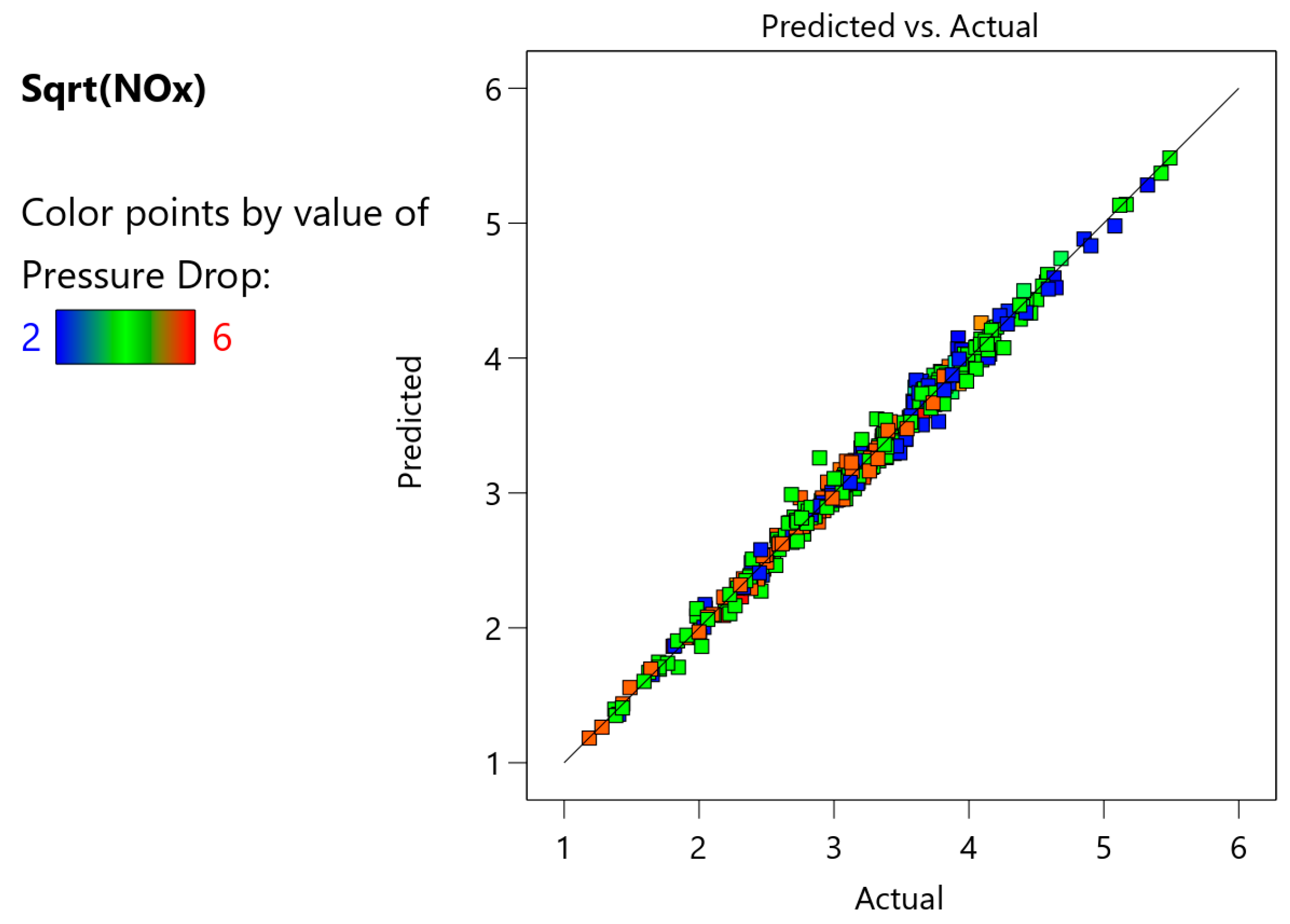
The resulting coded equation from the model, i.e., NOx prediction in terms of the factor levels coded between −1 and 1, was used to compute the NOx emissions for the 398 data points from the study, and these predictions were compared against the experimental measurements for a final assessment of the model (see Figure 6). To provide an understanding of the form of the correlation developed by ANOVA, the five most influential terms based on their F-values are shown in Equation (1). To carry out the ANOVA, the full version of the equation (159 terms) was used. The NOx predicted values have units of ng/J.

$$\sqrt{NOx}=-26.04-0.35 AC-0.25 A^2-0.28 A{C}^2+0.22 D^2-0.11 ABG+[\dots ]$$

(1)

where $A$ stands for the air split, $C$ for the air swirl, $D$ for the pressure drop, $B$ for the fuel swirl and $G$ for the adiabatic flame temperature.

An average deviation of 3.07 ng/J was obtained between the predicted and the measured emissions, corresponding to an error of 29.8% or an average accuracy of 70.2%.

3.2. Machine Learning Algorithm

Neural networks are widely used in combustion [1]; however, deep artificial neural networks typically work for larger data sets than the present. As a result, supervised machine learning models like random forest or AdaBoost are more appropriate with the current data set. In the present work, a random forest algorithm based on Python’s machine learning library, scikit-learn, was used. This supervised learning approach combines a series of tree predictors (or decision trees), each built from a subset of the total data set and making an independent prediction, and outputs a weighted average of the predictions from all of them. For a more detailed mathematical background on the random forest algorithm for prediction, check [21] as a reference.

The number of estimators was kept at 100; 80% of the data was used to train the model, and the remaining 20% was used for testing. The random forest regressor presented an R² training score of 0.97, an out-of-the-bag (OOB) error of 0.8, and an R² validation score of 0.75. The feature importance reflects the relative significance of each input variable in the training data (see Figure 7). In the following, features from the images are discussed. As expected with the previously established NOx and OH* intensity correlations (see Figure 4 from [9], where the research group displays a positive linear trend between the OH* chemiluminescence intensity and the measured NOx emissions), the average and maximum brightness presented importance values of 0.3153 and 0.1791, respectively, reflecting their relative impact on the model’s NOx predictions. These relative importance values are computed based on the decrease in model accuracy when the feature is used for splitting the data in the decision tree. These image features were followed in importance by the following: (1) the center of gravity downstream location (throughout [9], the authors used the concept of the location of the center of gravity as a way of representing the available time for mixing air and fuel: the farther from the injector plate, the greater time for mixing and therefore the lower the NOx emissions); (2) the pressure drop; (3) the heat release area and flame height, with importance values of 0.1319, 0.0962 and around 0.0346 the latter two, respectively. Of course, pressure drop is not an imaging-based feature and is discussed more below. A larger heat release area with high OH* chemiluminescence levels is consistent with higher NOx. The connection between the flame height and NOx is similar to that for the flame area. The influence of pressure drop is associated with the fact that these are not fully premixed reactions. Higher pressure drops result in higher mixing rates, which tend to reduce emissions from such non-premixed flames. The lack of significance of adiabatic flame temperature is again related to the non-premixed nature of these reactions. Non-premixed reactions have peak local flame temperatures at near stoichiometric conditions. The NOx emissions depend mainly on the peak local temperatures, which change so much depending on the conditions studied. Hence, the imaging-based features have more significance than the estimated adiabatic flame temperature. Regardless, the results illustrate the strong dependency on image-based features, which underscores the potential for using images to infer NOx behavior.

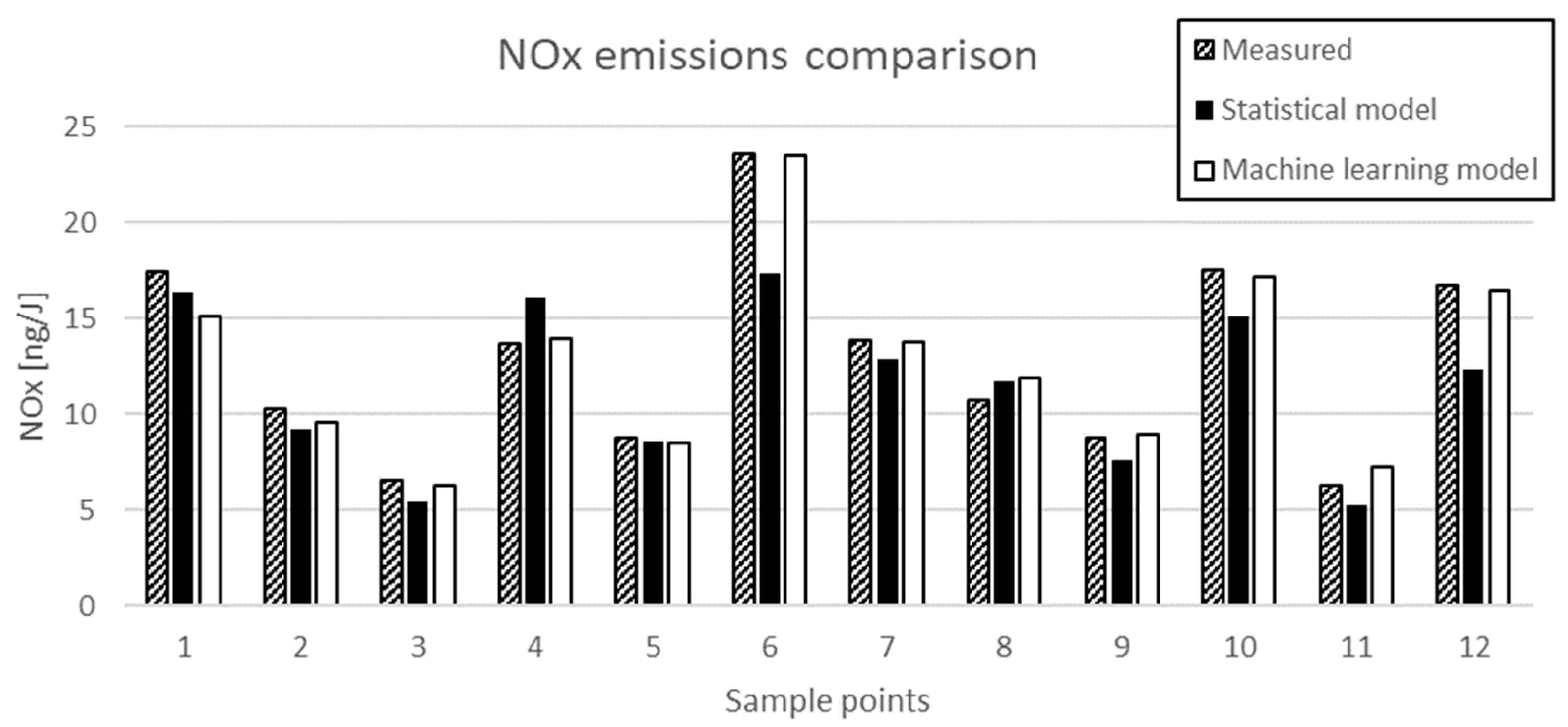
By comparing the predicted values of the test data against the experimental measurements, the average accuracy of the random forest model was 82.60%, representing an increase of 12.4% compared to the statistical approach. Figure 8 shows 12 data points from one of the sixteen injectors with comparisons between the measured NOx emissions and the two predictive models.

The resulting model was also used to estimate the best injector configuration to reduce the NOx emissions. This process is equivalent to the optimization exercise described in [9] in which the geometric configurations that minimized NOx while targeting minimum air pressure drops were sought. The ability of the ML model to indicate the preferred configuration to attain this optimization gas was therefore used as another way to validate the ML model. Therefore, the contribution of each of the three injector factors was averaged for each of their three levels (low, mid, high), and it was found that with high air split, low fuel swirl and high air swirl, the NOx emissions are diminished. This preferred combination of factors precisely aligned with the conclusions of the statistical model. An extra injector with these conditions was designed, manufactured and tested in a continuation work, and the predicted trend was confirmed [22].

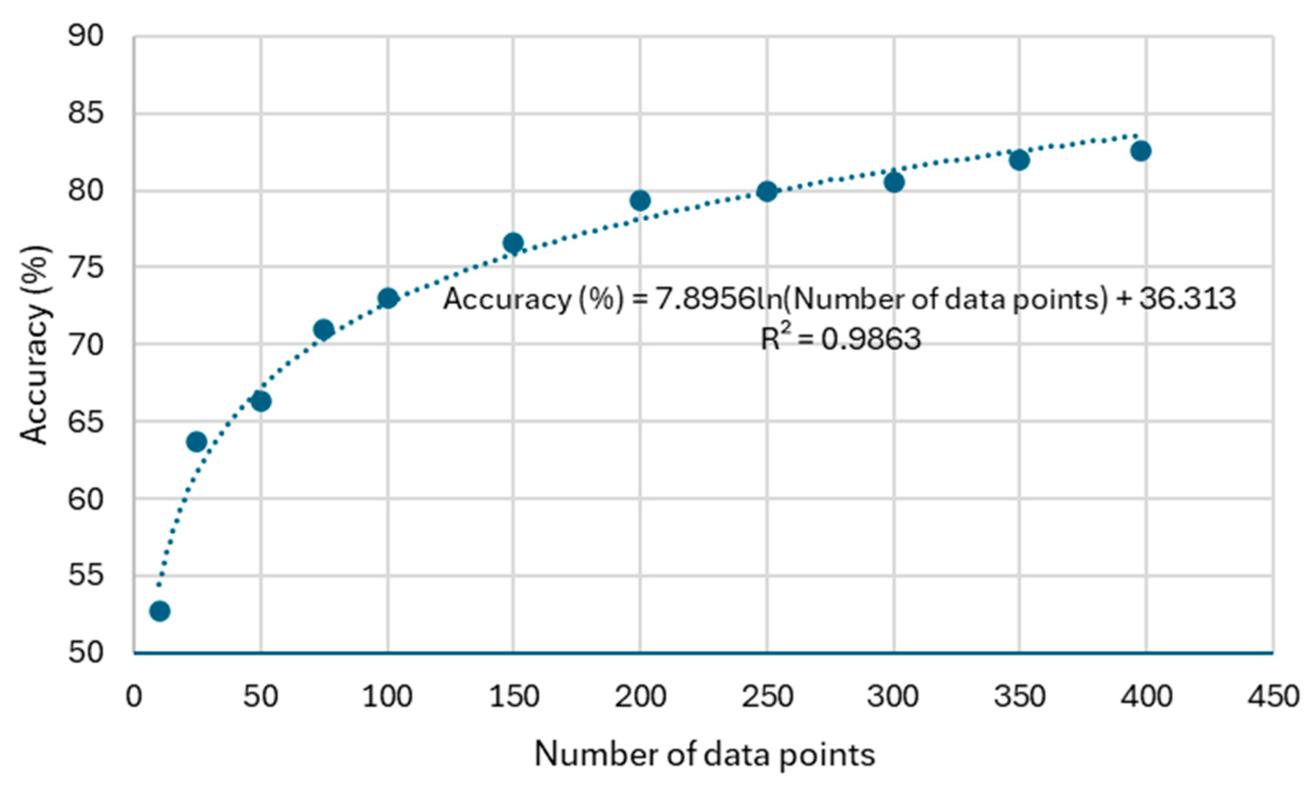
A divergence assessment of the model was conducted to assess its accuracy as a function of the number of used data points. The accuracy of each testing point was computed by subtracting the relative error from 100%, which is the relative error of the difference between the predicted and the measured NOx emissions over the measurement. The accuracy of the model is computed as the average of all data points.

The maximum number of data points was given by the available data points (398). Then, a randomly selected subset from the original data set was taken. Models with 350, 300, 250, 200, 150, 100, 75, 50, 25 and 10 points were analyzed. As expected, Figure 9 shows a logarithmic dependence between the accuracy of the model and the size of the data set.

3.3. Statistical Model and Machine Learning Algorithm Comparison

With the model results from each approach introduced, this section summarizes the main differences between the standard statistical model and the machine learning model. At a high level, a major differentiator is that the statistical model is based on a field of mathematics focused on the formalization of relationships between variables in the form of equations, whereas the ML model is based on a field of computer science building algorithms that learn from data for predictions or classifications.

Table 1. Key features comparison.

Factor	Statistical Model	Machine Learning
Preplanning	For statistical models to be successful, preplanning regarding reduction in colinear factors, balanced design space and range of factors is important. A wide range of strategies have been developed that account for these features but also provide an inherently efficient test matrix, as one of the goals of these methods is to allow the acquisition of maximum information with a minimum number of tests. In the present study, the Box–Behnken design allowed 13 hardware parts to be built instead of 27.	Minimal planning is required as long as an extensive amount of data is obtained. This makes ML analysis well suited for “after the fact” data. This is very attractive for the analysis of historical data, in which statistical methods were not used to set up the testing plan originally.
Data complexity and dimensionality	Suitable for simpler and low-dimensional data sets, establishing straightforward relationships.	Suitable for more complex models with high-dimensional data.
Feature engineering	Top-to-bottom approach, where assumptions of the data distribution need to be made. The current effort assumes the applicability of normal statistics, relying on a model with terms with statistical p-values lower than 0.05 and up to third order.	Bottom-to-top approach, where no particular models are assumed. Automatically handles the interactions and patterns that perform best (also referred to as data-driven). Machine learning can handle a larger number of variables, resulting in complex models.
Model interpretability	The model provides interpretable coefficients or parameters. In this case, the NOx emissions were described using an equation. The resulting terms of the model indicate whether the variables contribute positively or negatively to the overall result and allow a direct reading of the relative impact of the variables. From the 159 terms of the NOx equation (simplified in Section 3.1), the five most significant factors were the interaction between the air split and air swirl; the quadratic term of air split; the interaction between air split and quadratic term of air swirl; the quadratic term of pressure drop; and the interaction between the air split, fuel swirl and adiabatic flame temperature.	Machine learning models are typically referred to as “black boxes”, because of their lack of interpretability. Since the user does not build the model itself, one must rely on the resulting network and representative graphs of the features’ importance. In the current effort, the weights of each variable of the random forest algorithm are yielded in Figure 7. According to their feature importance or relative contribution to the predictive accuracy of the model, these are the top five most significant variables: average brightness, maximum brightness, center of gravity of the heat release area, pressure drop and preheat temperature. However, the main drawback of this approach is that the user does not have a direct sense of how each of them affects the model.
Generalization	When dealing with mid-to-large data sets, the resulting model is complex and often difficult to interpret because of the large number of factors and interactions. Moreover, it might be prone to overfitting, so the generalization process would be negatively affected.	For properly regularized and validated models, the algorithm can perform well on new, unseen data. This is well reflected in the accuracy obtained with the test data set, a subset that was not part of the training set used to build the model.
Training time	For the current effort, Design Expert was used to perform the statistical analysis. The data were already prepared in a table format, so the input process was immediate. The statistical computations were instantly performed by the software, so the training time relied on the adjustment of the model parameters.	Equivalently to the statistical analysis, the training time for this particular work was not critical since the Python code and libraries that were used performed all the calculations in minimal time.
Prediction accuracy	The statistical model yielded an accuracy of 70.2%.	The machine learning algorithm yielded an accuracy of 82.6%.
Overall performance	Because of the complexity of the resulting non-linear model, the interpretability of factors is limited. The scalability for large-scale applications and generalization are critical limitations of the system.	The model adapts to complex non-linear relationships and high-dimensional data coming from imaging diagnostics. Despite the lack of interpretability, the features’ importance can be used to obtain a basic understanding of the relevance of each variable.

compares the key features of each approach as directly applied to this specific study.

4. Conclusions

The present work compares predictive models for NOx derived from images of flames, injector geometry and test conditions. A set of 16 injectors was designed according to a statistically distributed space with varying air split, fuel swirl and air swirl. These were tested for different air flows, fuel flows, fuel compositions and flame temperatures. This yielded 398 data points, which were used to generate both statistical and random forest models.

Regardless of the originally intended statistical approach, it was found that the machine learning algorithm could predict the NOx emissions with higher accuracy (82.63%) compared to the analysis of variance approach (16.33% improvement). As opposed to the statement from [1], even with a small amount of data, it was observed that the machine learning approach performed better than the classical, multivariate statistical model. The average relative error of 17.37% is promising compared to the uncertainty of the system itself, stated at 11.1%, and emphasizes the need for further research and development in this field. It is noted that the data set used for ML analysis was small compared to the typical sizes used to train machine learning algorithms. Considerable improvement would be expected by enlarging the number of data points to train and test the models. Yet, ironically, the acquisition of these additional data would require considerably more time and cost.

In summary, both modeling approaches yielded similar conclusions relative to the preferred injector configurations to minimize NOx. One observation is that the statistical model approach relies more on preplanning than the ML method. It is also noted that the results here, while demonstrated using experimental test results, could also be relevant to data generated by CFD methods.