Article

Numerical and Experimental Investigations on the Acoustic Characteristics of a Single-Stage Centrifugal Pump †

1
Department of Mechanical Engineering, TU Dortmund University, 44227 Dortmund, Germany
2
Department of Mechanical Engineering, Ruhr University Bochum, 44801 Bochum, Germany
*
Author to whom correspondence should be addressed.
This paper is an extended version of a conference paper published in the Proceedings of the 15th European Turbomachinery Conference, Budapest, Hungary, 24–28 April 2023; paper n. ETC2023-325.
These authors contributed equally to this work.
Int. J. Turbomach. Propuls. Power 2024, 9(1), 8; https://doi.org/10.3390/ijtpp9010008
Submission received: 6 December 2023 / Revised: 17 December 2023 / Accepted: 3 January 2024 / Published: 1 March 2024

Abstract

:
The acoustic properties of a single-stage centrifugal pump with low specific speed are investigated by means of compressible 3D CFD simulations (URANS) and experiments. In order to determine the pump’s acoustic transmission and excitation characteristics, a four-pole approach in the frequency domain is used. The transmission parameters determined by simulation are compared to experiments in water and air as functions of the Helmholtz number. The results indicate that the acoustic transmission characteristics within the experiments are significantly influenced by the structural compliance of the volute casing in terms of a fluid–structure interaction (FSI). A modelling approach for a one-dimensional representation of the centrifugal pump’s acoustic transmission characteristics in the time and frequency domains is applied to the current pump. As one model parameter, the effective speed of sound in the 1D model needs to be reduced to 607 m s 1 to account for the FSI. The agreement of the simulation results and the experiments underlines the above statement about the influence of the FSI. In a last step, the acoustic excitation parameter, depicted as monopole and dipole amplitudes, at two different blade-passing frequencies ( f B P [ 111 ; 169 ] Hz) are determined for several operating points. Especially for dipole amplitudes, a good agreement between experiments and simulations can be seen. The monopole amplitudes are also of similar orders of magnitude, but show stronger deviations. The cause of discrepancies between the 3D CFD simulations and experiments is believed to be the neglected influence of the FSI and surface roughness as well as the inaccurate reproduction of flow separation at the volute’s tongue due to the use of wall functions. A final important observation made during the numerical investigations is that the excitation mechanisms at the blade-passing frequency are probably independent of the piping system’s acoustic impedance.

1. Introduction

A centrifugal pump has two main acoustic characteristics [1,2]. One is the active generation of pressure pulsations. The other one is the passive transmission and reflection of sound waves propagating from the connected piping system into the pump’s suction or discharge flange opening, respectively. Excited pressure pulsations can have broadband and tonal characteristics. Broadband excitation mechanisms are, e.g., turbulence or cavitation [3]. Tonal pressure pulsations appear as sharp peaks in the spectrum, mainly at the rotational frequency and the blade-passing frequency f B P and their higher harmonics. Especially in radial centrifugal pumps with volute casings, the pulsations at the f B P are of the highest amplitudes [4]. The occurrence of pressure pulsations at the f B P is due to two basic effects. Both result from the fact that an impeller rotates in a fixed casing. For an observer inside the housing right next to the impeller outlet, pressure and velocity alternate at f B P . Because of that, the circulating pressure [5] and velocity fields [3,6] within the impeller are primary sources which represent the two basic effects mentioned above. Furthermore, the fluctuating velocity field interacts in particular with the volute’s tongue [7]. This rotor–stator interaction (RSI) results in an equivalent acoustic dipole source [8]. In the first instance, the sources’ strengths depend on the operation point and rotational speed. Apart from this knowledge about sound generation mechanisms, the question of whether the acoustic sources in a centrifugal pump are independent of the acoustic impedance of the system to which the pump is connected remains partially unanswered so far.
As indicated at the beginning, another important acoustic characteristic of centrifugal pumps is the transmission and reflection of incoming acoustic pressure waves. This passive behaviour is, in general, pump-specific and frequency-dependent. It is partly influenced by the pump’s inner geometry, i.e., the inner fluid volumes or rather cross-section jumps and corresponding lengths. As another influencing parameter, the structural compliance of the casing is supposed to have a significant impact on the transmission behaviour. This is justified by the fact that the effective speed of sound within the pump’s casing is reduced in comparison to the effective speed of sound in the connected piping system. An abrupt change in the speed of sound leads to a proportional change in the acoustic impedance, which, finally, leads to a higher reflective pump transmission behaviour [8,9].
The measurable pressure amplitudes in the piping system on the suction and discharge side of the pump are always an outcome of the pump’s acoustic behaviour and the acoustic impedance of the piping system. In order to determine the acoustic transmission and excitation characteristics, a special measurement procedure is necessary. Since the range of frequencies considered in this investigation is far below the frequencies of higher-order modes, pipeline acoustics can be considered as one-dimensional. With this assumption, it is possible to evaluate the acoustic pressure fields on both sides of the pump by means of pressure measurements in the piping system [10]. At least two probes on each side are needed to decompose the measured information in up- and downstream-propagating acoustic pressure waves. Based on this pressure field decomposition, the pump’s acoustic characteristics can be quantified. Therefore, the pump is considered as a black box, or rather an acoustic four-pole, which connects the up- and downstream-propagating pressure waves from both sides. Based on this system-theoretic approach, the acoustic transmission parameters are determined first. In a following step, the pump’s excitation parameters can be quantified in the form of complex monopole and dipole amplitudes. Under the assumption that these parameters are independent of the connected piping system’s acoustic impedance, (this assumption was investigated experimentally for a comparable single-stage centrifugal pump in [8] by investigating the influence of a connected Helmholtz resonator on the monopole and dipole sources of the pump for selected operation points. While the dipole sources were hardly affected by the change in system impedance caused by the resonator, the monopole sources were more strongly influenced. The reason for the changed monopole source strengths as a result of the impedance change has not yet been clarified. Accordingly, the assumption of system-independent excitation parameters has not yet been confirmed experimentally. It is possible to compare, for example, the acoustic characteristics of a pump based on CFD simulations and experiments. To the authors knowledge, no such comparison has been made so far. If it is feasible to achieve quantitatively comparable acoustic excitation parameters by means of CFD simulations, the four-pole method used in this work could help to acoustically validate CFD pump models in the future. This is particularly important as the current validation technique of such models in the literature has so far been limited to the comparison of steady state experimental characteristics. Even if these models are to be used to investigate acoustic variables and correlations in the pump.
In previous works, a one-dimensional model was developed which is capable of representing the acoustic characteristics of single-stage centrifugal pumps with volute casings in the time domain [8,9]. To model the pump’s acoustic transmission behaviour, both the pump-specific inner geometry and the compliance of the casing, in the sense of a reduced effective speed of sound, are taken into account. It was highlighted that the reduction in sound speed depends in particular on the casing’s geometric shape and, therefore, to a certain extent on the pump’s specific speed [9]. Even if the capability of this one-dimensional approach was used for different pumps successfully, an experimental verification of the influence of the fluid–structure interaction (FSI) is still missing.
The present study is based on a combined experimental–numerical approach to analyse the acoustic transmission and excitation behaviour of a single-stage centrifugal pump with a volute-type casing and represents an extension of the conference paper [11]. The focus can be divided into two main questions, which are unanswered to the authors’ best knowledge. First question: To what extent does the FSI, i.e., the coupling between fluid pressure pulsations and structural compliance of the pump’s casing, influence the pump acoustics? Second question: Are the pump excitation parameters, determined by means of the measurement procedure, and concomitantly the underlying source mechanisms, independent of the connected pipeline system? To analyse the first question, experimentally assessed transmission parameters in water and air are compared to simulated ones (CFD). Furthermore, in order to determine how the inner geometry and effective speed of sound in the pump influence its transmission parameters, a one-dimensional model, by means of the approach used by [8], is developed in the time and frequency domains (MOC and TMM). For CFD simulations, no FSI is taken into account. This provides a model which includes all the effects of three-dimensional pressure wave reflection and transmission in the pump, without the simultaneous influence by structural effects. The same applies to measurements in air. For validation, the one-dimensional model is first compared to CFD simulations and experiments in air to check the geometric approximation. Afterwards, the effective speeds of sound within the pump are calculated based on static mechanical FEM simulations. The results are used as input parameters for the ”compliant” one-dimensional pump model. The transfer parameters are calculated and compared to experiments in water. In the next step, excitation parameters for experiments in water and CFD simulations are determined based on the known particular transmission behaviour, normalised and compared for varying flow rates and two rotational speeds. Further, CFD simulations of several operating points are recalculated with modified acoustic system impedances to study the second question.
The paper is structured as follows. First, a brief fundamental introduction to the determination of acoustic pump parameters is given. Thereupon, the experimental, numerical, and 1D model approaches are introduced. In the following section, the results for the acoustic quantities are discussed in detail, with an emphasis on the defined research questions, before the paper is concluded with a summary of insights gained.

2. Methods and Approaches

2.1. Determination of Acoustic Pump Parameters

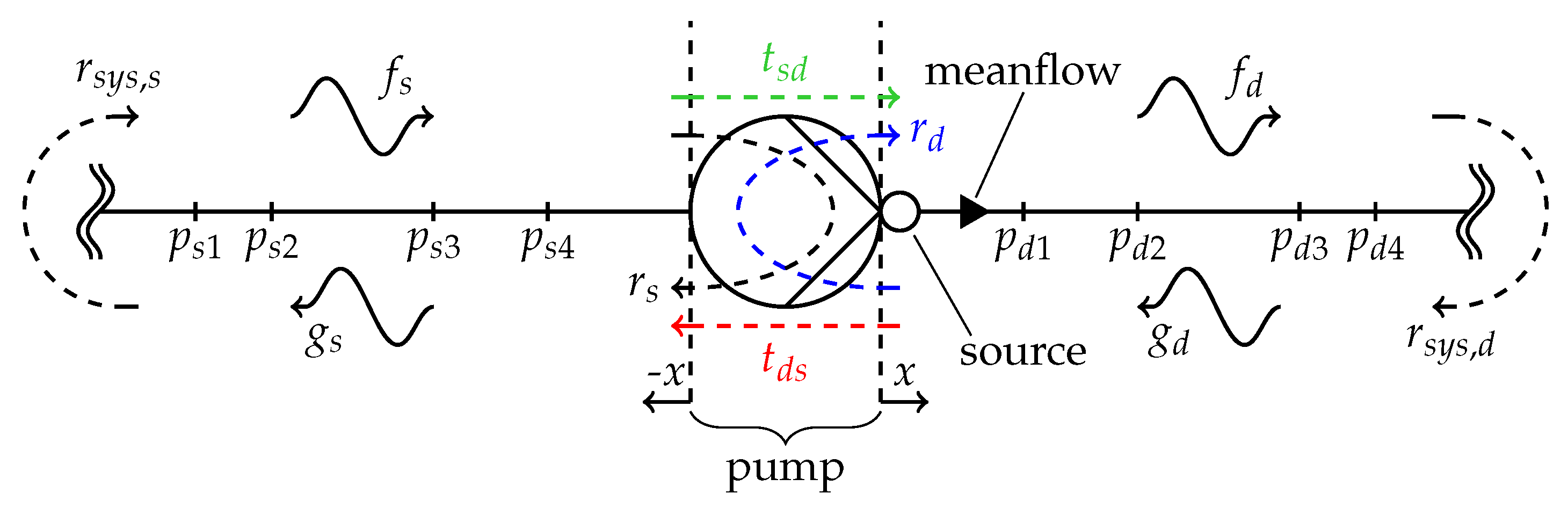
In order to quantify the transmission and excitation parameters, the pump is interpreted as an acoustic four-pole in the frequency domain. This system-theoretic approach is applied to the experiments and CFD simulations within this study. In Figure 1, a schematic representation of the pump’s acoustic surrounding is shown. By means of the linear equation
f ^ ̲ d g ^ ̲ s = t ^ ̲ s d r ^ ̲ d r ^ ̲ s t ^ ̲ d s S ̲ ̲ f g f ^ ̲ s g ^ ̲ d + f ^ ̲ s r c . + r ^ ̲ d g ^ ̲ s r c . t ^ ̲ d s g ^ ̲ s r c . ,
the following parameters are connected:
  • f ^ ̲ s , g ^ ̲ s and f ^ ̲ d , g ^ ̲ d : up- and downstream-propagating pressure waves, with f ^ ̲ and g ^ ̲ quantifying the acoustic pressure fields on the suction (s) and discharge (d) side of the pump,
  • S ̲ ̲ f g : the pump’s scattering matrix, which contains the four transmission parameters r ^ ̲ s , t ^ ̲ s d , r ^ ̲ d , and t ^ ̲ d s ,
  • f ^ ̲ s r c . and g ^ ̲ s r c . : the pump’s source (src.) parameters in the form of up- and downstream-propagating pressure waves.
Generally, if the acoustic pressure fields in the pump’s suction and discharge piping are known, the requested pump parameters can be inferred. To decompose a one-dimensional acoustic pressure field in up- and downstream-propagating waves f ^ ̲ and g ^ ̲ , the complex pressure amplitudes p ^ ̲ ( x ) at a minimum of two different locations along the direction of propagation x must be known [12]:
p ^ ̲ ( x 1 ) p ^ ̲ ( x m ) y = e i k x 1 e i k x 1 e i k x m e i k x m A ̲ ̲ f ^ ̲ g ^ ̲ x with k = 2 π f a e f f , t
where k is the frequency (f)-dependent wave number. Wave propagation is assumed to be lossless, without convective components, and linear. The fluid is considered single-phase. The effective speed of sound in the piping a e f f , t is assumed to be frequency-independent. A first and good (based on our experience in measuring the propagation of sound waves in thin-walled, water-filled steel pipes) estimation of a e f f , t in an elastic, axially fixed pipe can be calculated according to [13] by means of
a e f f , t = a f 1 + E f ( 1 ν 2 ) E t × d s .
where E t and ν are the Young’s modulus and Poisson’s ratio of the pipe material, s is the wall thickness, d the inner pipe diameter, and a f and E f are the fluid’s specific speed of sound and Young’s modulus. For compressible single-phase CFD simulations without taking FSI into account, a e f f , t equals the fluid specific speed of sound a f . If the number of measuring points is m > 2 , Equation (2) becomes overdetermined. Especially for experiments, this is desirable to compensate for measurement errors. In this case, f ^ ̲ and g ^ ̲ need to be determined by means of a least squares method. For this, both sides of Equation (2) are multiplied by the complex conjugate transposed (adjoint) matrix A ̲ ̲ H to obtain the Gaussian normal equation
A ̲ ̲ H y = A ̲ ̲ H A ̲ ̲ x
and, therefore, a solvable linear system of equations [14]. In order to evaluate the quality of the solution found, a relative error ϵ r e l , based on the residuum f ^ ̲ e i k x + g ^ ̲ e i k x p ^ ̲ ( x ) , is determined
ϵ r e l = n = 1 m | f ^ ̲ e i k x n + g ^ ̲ e i k x n p ^ ̲ ( x n ) | 2 m × p ^ m a x 2 × 100 % with p ^ m a x = | f ^ ̲ | + | g ^ ̲ |
Since the effective speed of sound a e f f , t should be a result of the procedure as well, a superior golden-section search algorithm [14] is prepended to the least squares method described above to find the value of a e f f , t within a defined range which minimises the residuum. By means of this optimisation procedure it is now possible to evaluate a e f f , t , f ^ ̲ and g ^ ̲ and, therefore, the requested acoustic pressure field parameters in the pump’s suction and discharge piping. Note that the system’s reflection coefficients r ^ ̲ s y s , s and r ^ ̲ s y s , d can be calculated by means of
r ^ ̲ s y s , s = f ^ ̲ s g ^ ̲ s and r ^ ̲ s y s , d = g ^ ̲ d f ^ ̲ d
Based on the known in- and output parameters f ^ ̲ s , g ^ ̲ s , f ^ ̲ d , and g ^ ̲ d , the four-pole’s unknown transmission parameters r ^ ̲ s , t ^ ̲ s d , r ^ ̲ d , and t ^ ̲ d s can be determined. It can be assumed that the transmission behaviour of the pump in standstill corresponds in a good approximation to that of the pump in operation [15]. Since in standstill f ^ ̲ s r c . = g ^ ̲ s r c . = 0 , Equation (1) is simplified. It is then possible to estimate S ̲ ̲ f g using at least two different sound configurations m 2 on each side of the system:
f ^ ̲ d 1 f ^ ̲ d m g ^ ̲ s 1 g ^ ̲ s m = t ^ ̲ s d r ^ ̲ d r ^ ̲ s t ^ ̲ d s f ^ ̲ s 1 f ^ ̲ s m g ^ ̲ d 1 g ^ ̲ d m
The two-source method is the most effective way to create different sound configurations. By means of alternating the sources’ amplitudes and phases relative to each other it is theoretically possible to generate an infinite number of linear independent configurations [16]. If Equation (7) is overdetermined ( m > 2 ), the transmission parameters can be evaluated by means of the same least squares method approach used to solve Equation (2) for m > 2 .
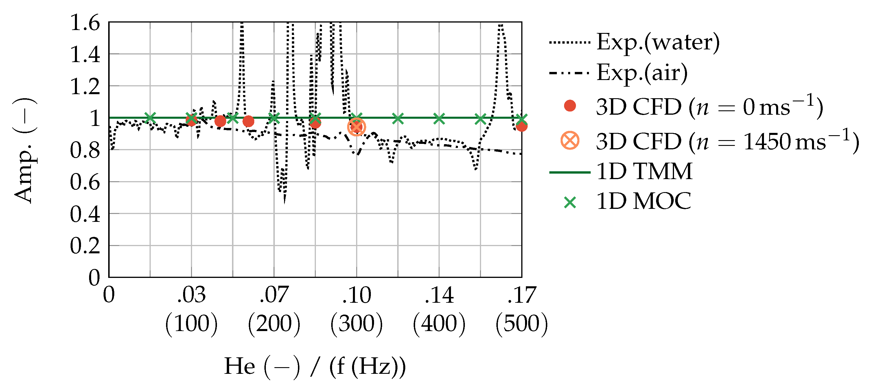
If it is additionally to be investigated whether a four-pole tends to have dissipative, passive, or active properties, the acoustic power ratio ζ can be calculated. ζ is the ratio of outgoing and incoming time-averaged acoustic powers and can be determined from the transmission parameters:
ζ = P ¯ o u t P ¯ i n = r ^ s 2 + Z t , s Z t , d t ^ s d 2 + r ^ d 2 + Z t , d Z t , s t ^ d s 2 2
Z t , s and Z t , d are the acoustic impedances within the pipes connected to the suction and discharge flange of the pump. The derivation of Equation (8) is shown in Appendix A. Based on the amount of ζ compared to one, the following conclusions can be drawn:
  • ζ < 1 : the part different to one is dissipated (or transformed) within the four-pole;
  • ζ = 1 : the four-pole is a purely passive acoustic element;
  • ζ > 1 : the part different to one is generated (or transformed) within the four-pole.
Ideally, the acoustic transmission behaviour of the pump should be purely passive. This is the special case for a pump in standstill in the absence of dissipative and FSI effects. Therefore, the evaluation of ζ is used herein to analyse the quality of the CFD simulations regarding numerical dissipation of acoustic pressure waves and the effect of the FSI on the experimentally determined transmission parameters.
Looking back on Equation (1), the only unknown parameters left are the up- and downstream-propagating source waves f ^ ̲ s r c . and g ^ ̲ s r c . . In order to estimate a set of source parameters, f ^ ̲ s , g ^ ̲ s , f ^ ̲ d , and g ^ ̲ d need to be determined while the pump works in a specific operation point. By means of the following Equation f ^ ̲ s r c . and g ^ ̲ s r c . can be transformed into the native acoustic sources monopole p ^ ̲ s r c . and dipole c ^ ̲ s r c . to allow a better physical interpretation:
p ^ ̲ s r c . = f ^ ̲ s r c . + g ^ ̲ s r c .
c ^ ̲ s r c . = ( f ^ ̲ s r c . g ^ ̲ s r c . ) 1 z s r c . with z s r c . = ρ f · a e f f , s r c . .
where z s r c . represents the specific acoustic impedance in the source region and is calculated using the corresponding effective speed of sound a e f f , s r c . .

2.2. Experimental Approach
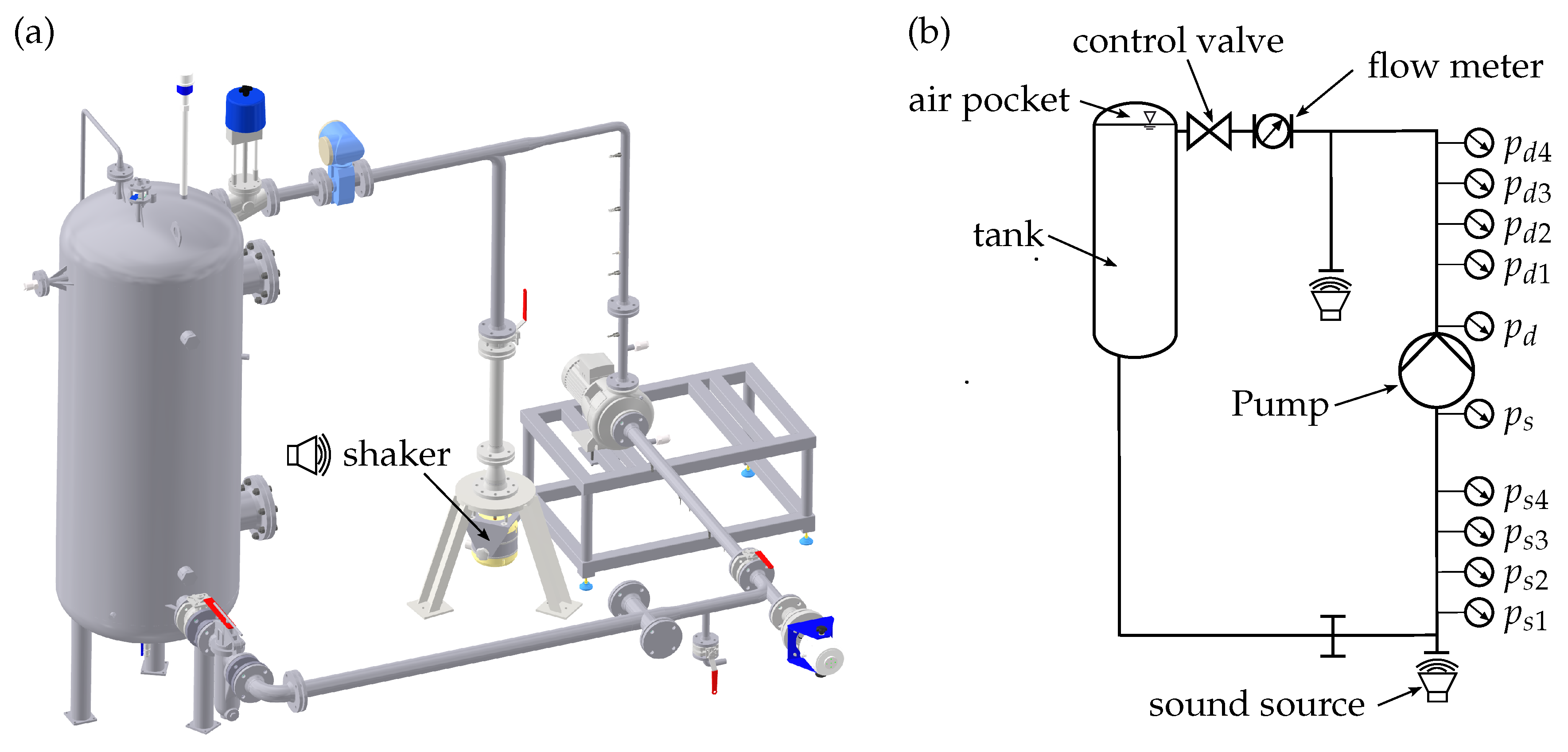
In Figure 2, the experimental setup is illustrated. The pump under test is a radial, single-stage centrifugal pump with a volute-type casing. The pump is speed-regulated and the specifications are listed in Table 1. For high-resolution pressure measurements in water, piezoelectric (PE) transducers Kistler™ (Winterthur, Switzerland) 7061 B/C are flush-mounted to the pipes’ inner walls on the suction ( p s 1 p s 4 ) and discharge ( p d 1 p d 4 ) sides of the pump.
The charge signal outputs of the PE sensors are amplified by means of Kistler™ (Winterthur, Switzerland) 5018A and 5011B charge amplifiers. For equivalent measurements in air, condenser microphones PCB™ (Depew, NY, USA) 130A23 are used. Sensor locations relative to each other are non-equidistant and optimised to the range of frequencies investigated in this study. In Table 2, measurement positions relative to the pump’s flanges are catalogued (flow direction = positive x-direction). Two capacitive pressure sensors STS™ (Sirnach, Switzerland) ATM 1st ( p s , p d ) and a magnetic inductive flow meter E+H™ (Reinach, Switzerland) Promag W are used to measure the pump’s head curve. A control valve is applied to adjust the pump’s operation point. An air pocket within the tank can be pressurised to regulate the system’s net positive suction head N P S H A . The value of N P S H A was set to 50 m to prevent cavitation in the pump as far as possible. Electromagnetic shakers (TIRA™ (Schalkau, Germany) TV 51110 and 51140-M) connected to a flexible membrane construction (water) or common loudspeakers (air) are used as optional sources of sound. All signals are further processed by means of the data acquisition devise imc™ (Berlin, Germany) Cronos Flex. Signals of PE sensors are sampled at 20 kHz and further post-processed by a flat-top windowed discrete Fourier transformation (DFT) with a uniform signal length of 16 s . The resulting frequency resolution is 0.0625 Hz . The useful frequency range of PE transducers and charge amplifiers is not limited to small frequencies, as they can also be used for quasi-static measurements. The microphones are calibrated for frequencies within 20 Hz f 20 kHz. The relative error ϵ r e l (Equation (5)) is used for a quality check of the measurement results since all further acoustic parameters are calculated based on the results for the pressure field decompositions.
The two-source method is used to evaluate the pump’s acoustic transmission characteristics (Equation (7)). The external sound sources (shakers or loudspeakers) are fed with a white-noise signal designed for the frequency range 10 Hz f 500 Hz . An attempt was made to generate as many different sound configurations as possible in order to minimise the influence of statistic measurement errors on the requested parameters.
Therefore, the sources’ amplitudes and the correlation of signals are varied to generate a number of m = 8 different cases. The evaluated results ( r ^ ̲ s , t ^ ̲ s d , r ^ ̲ d , t ^ ̲ d s ) are filtered by means of a weighted averaging function over five data points to statistically smooth the curves. Except for a few outliers ( 5 % < ϵ r e l < 10 % for frequencies around the system’s mechanical resonances) the relative error in decomposition applies ϵ r e l < 5 % for a e f f = 1350 10 + 10 m s 1 , which indicates good quality.
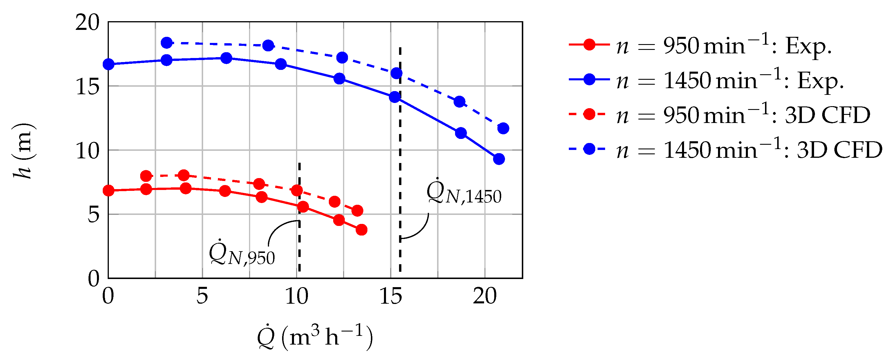
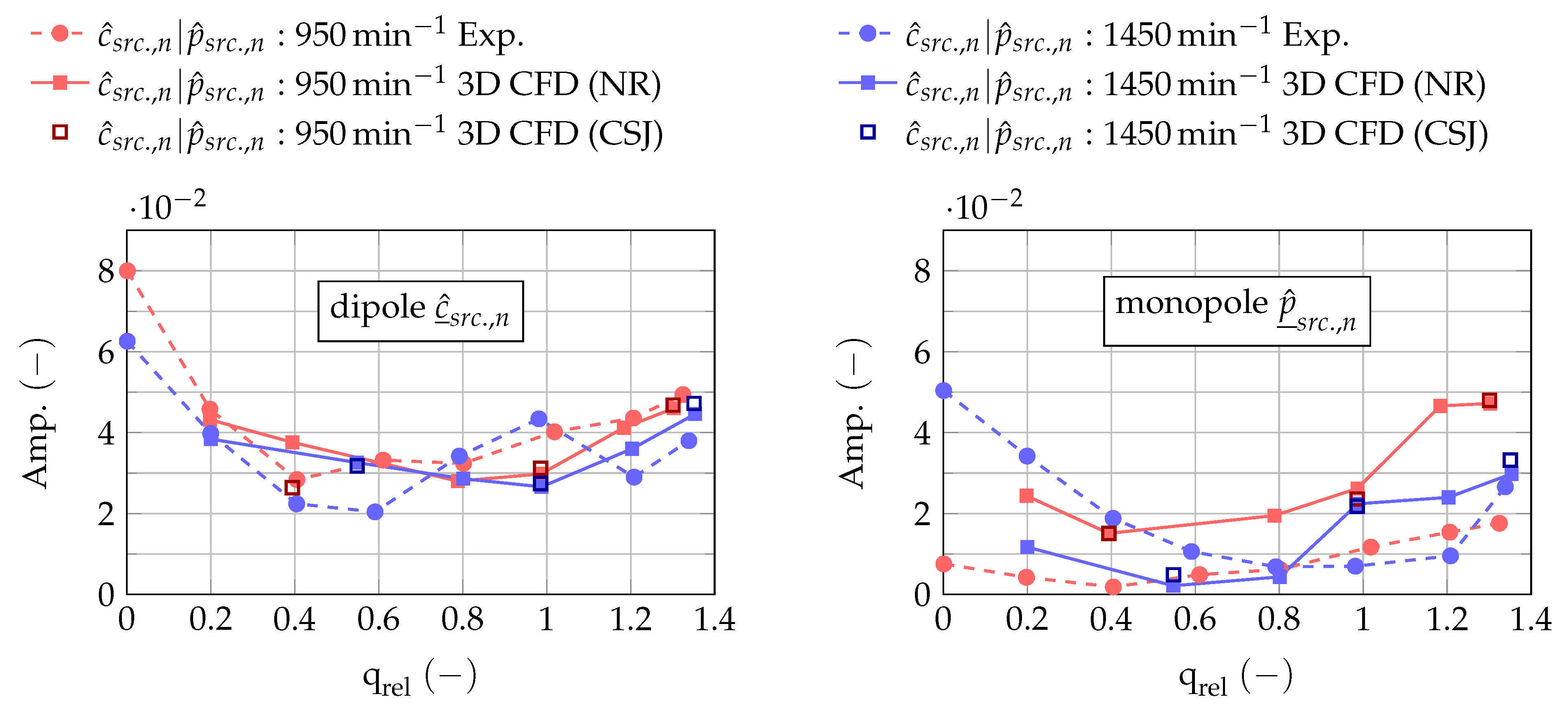
Finally, the source parameters are evaluated. The relative flow rate q r e l = Q ˙ Q ˙ N is varied in equal steps Δ q r e l = 0.2 from q r e l = 0 to the highest overload operation point of q r e l = 1.4 for two different rotational speeds ( n = 950 and 1450 m i n 1 ). For every single operation point the pressure field parameters f ^ ̲ s , g ^ ̲ s , f ^ ̲ d , and g ^ ̲ d are determined. The relative error in decomposition is again ϵ r e l < 5 % for a e f f = 1350 10 + 10 m s 1 . Based on that, as well as on the known transmission parameters, the up- and downstream-running source waves f ^ ̲ s r c . and g ^ ̲ s r c . are calculated (Equation (1)) and further transformed into complex monopole p ^ ̲ s r c . and dipole c ^ ̲ s r c . amplitudes (Equations (9) and (10)).

2.3. 3D CFD Approach

An in-house CFD solver named solver3D is used to calculate the pump’s flow-acoustic behaviour. It is described in detail by [17,18] and is summarised here only very briefly. The unsteady Reynolds-averaged Navier–Stokes (URANS) equations are solved by a cell-centred unstructured finite volume (FV) scheme. The extended SIMPLE (semi-implicit method for pressure-linked equations) algorithm for compressible flow is used. The accuracy of the interpolation approaches used is second-order in space. An implicit three-level time discretization scheme is employed, which is second-order accurate as well. The flow is further assumed to be isothermal. Single-phase flow is applied, which means that cavitation effects are omitted. The Tait equation for liquid water is applied as a barotropic equation of state (EOS). The speed of sound is assumed to be a f = 1482 m s 1 for ambient temperature T f = 293 K and density ρ f = 998 k g m 3 .
The simulation setup is adopted from [19]. The statistical shear stress transport (SST) turbulence model with automatic wall treatment is used.
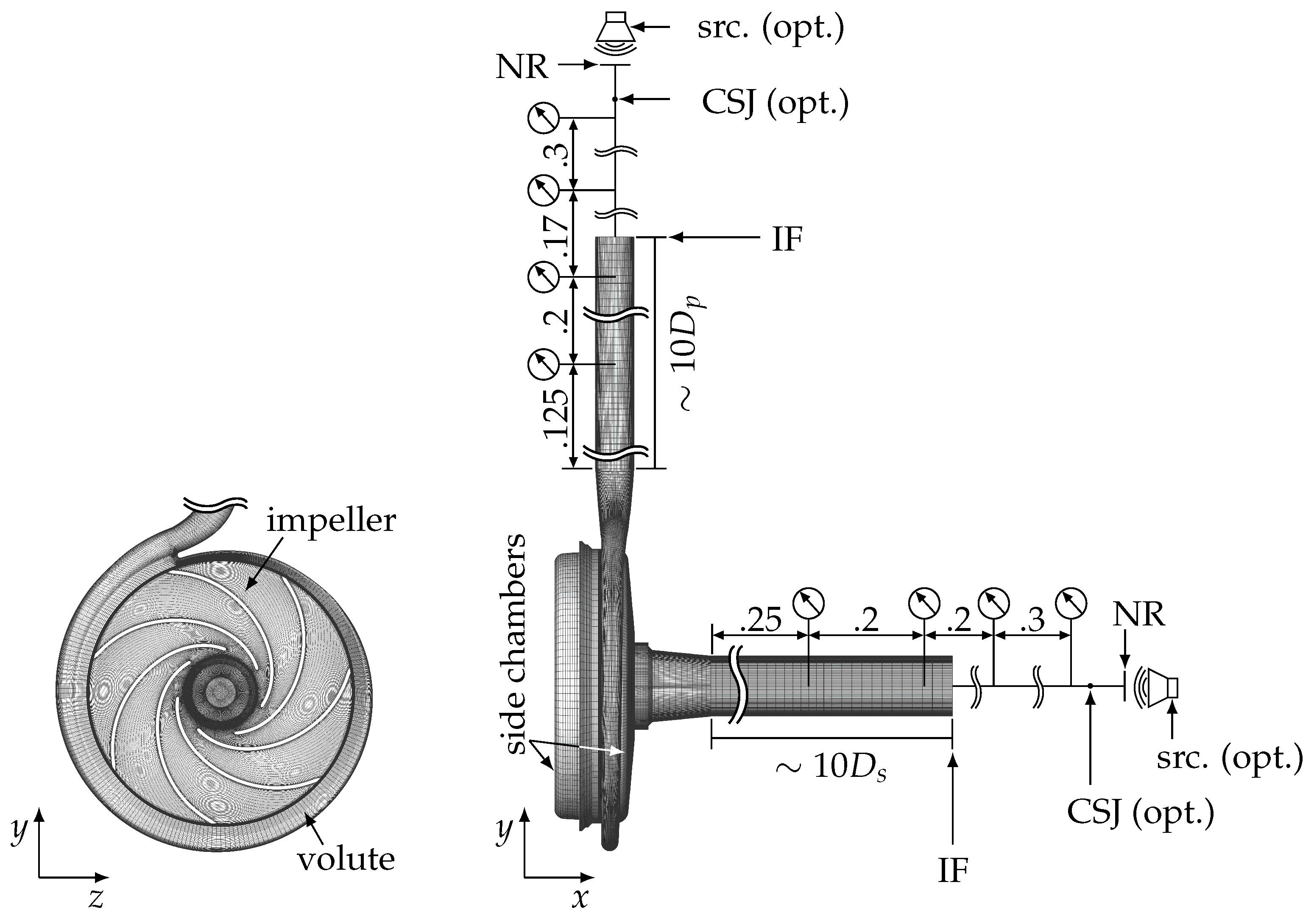
The 3D domain is illustrated in Figure 3 and consists of impeller, volute casing, side chambers on the suction and pressure sides, as well as pipe sections beyond the pump’s suction and discharge flanges. The structure surrounding the fluid is considered rigid, namely, no FSI is taken into account. According to previous investigations, the pump’s head is grid-independent for a grid with about 2 million hexahedral cells when wall functions are used. The latter simplification leads to an over-prediction of the pump’s head, especially in overload operation, which can be attributed to an inaccurate reproduction of flow separations at the volute’s tongue [19,20]. However, the computational effort for the resolution of a viscous boundary layer ( y + 1 ) combined with high time resolution requirements would be exceptionally high and is, therefore, out of this research’s scope. A sliding mesh interface is used to connect the rotating impeller with the stationary casing part. A time resolution of about 0.1 ° impeller rotation is prescribed to ensure a proper resolution of the acoustic pressure wave propagation. This corresponds to a time step of Δ t = 1.6 × 10 5 s for n = 1450 m i n 1 . For the lower rotational speed n = 950 m i n 1 , the same time-step size is adopted, leading to a time resolution of 0.066 ° impeller rotation. The acoustic Courant–Friedrichs–Lewy (CFL) number, calculated by means of
C F L a c = ( a f ± c ) Δ t Δ x ,
where c is the mean velocity of the fluid, is about C F L ¯ a c 10 on average and has a maximum value of C F L a c , m a x 200 . As depicted in Figure 3, the 3D-FV area is coupled to a 1D finite difference (FD) domain at the interface (IF). The coupling is employed since a non-reflecting (NR) boundary condition (BC) is integrated within the 1D code. The NRBC is prescribed at both ends of the 1D domain. This makes it possible to selectively adjust the system impedance by an optional cross-section jump (CSJ) before the NRBC. The numerical scheme is based on the one-dimensional conservation equations for mass and momentum in characteristic form (method of characteristics (MOC)). It is implemented in the in-house solver FLOAT [8]. The 3D/1D coupling in terms of the pump model used is set and analysed in detail by [18] according to the procedure in [21].
The method for evaluation of the acoustic parameters is adapted from experiments:
(i)
the pump is left at standstill and treated with sound from external sources (src.) to evaluate the transmission parameters;
(ii)
several operation points are adjusted to calculate the monopole and dipole amplitudes from the CFD simulations.
In both cases, monitor points in the 3D domain are used to record the high-resolution pressure–time signals, which are further flat-top windowed and transformed by a DFT for the acoustic pressure wave decomposition (Equation (2) with m = 2 ). Only time intervals with constant pressure amplitudes, are used for further evaluation. Each time interval has a length of 28 periods minimum. For case (i) a sinusoidal pressure signal is prescribed at one boundary while the other one is kept solely non-reflective and vice versa. It follows that for each frequency of interest two independent configurations are generated to evaluate the related transmission parameters (Equation (7) with m = 2 ). In case (ii), the pump operates either in a fully non-reflective system (no CSJ, r ^ s , s y s = r ^ d , s y s = 0 ) or for equivalent operation conditions in a partly reflecting system (with CSJ, r ^ s , s y s = r ^ d , s y s = 0.6 ) to analyse the influence of varying the system impedance. The operating points are adjusted by means of prescribed mean flow at the inlet and mean pressure at the system’s outlet. Both boundary conditions are set in addition to the NRBC. Note that the decisive criterion for the length of the signal time intervals in case (ii) is the respective blade-passing frequency f B P , which is f B P = 111 Hz for n = 950 m i n 1 and f B P = 169 Hz for n = 1450 m i n 1 . As described above, a minimum of 28 periods of the signal is used for post-processing.

2.4. 1D Modelling

The approach described by [9] is used to develop a 1D model which represents the pump’s acoustic transmission characteristics in a frequency range of 0 Hz < f 500 Hz . Therefore, the geometry of the pump is simplified as a series connection of three one-dimensional elements: namely, suction port (SP), a middle part called chamber (CH), and discharge port (DP). Every element is geometrically defined via its diameter d and length l. The latter is to be understood as an effective acoustic length which corresponds to the average distance that pressure waves travel through the respective pump part. In the cases of the suction and discharge ports, the determination of the acoustic lengths l S P and l D P is straightforward since there is only a single path for plane pressure wave propagation. In order to calculate the acoustic length for the middle part, including the impeller and volute l C H , an effective acoustic length is determined. This corresponds to the average of the longest and shortest paths through the pump sections involved. The diameters of each model part d S P , d C H , and d D P are estimated by means of the respective fluid volumes V and the known acoustic length:
d = 4 V π l
In addition to the geometric model parameters, the effective speed of sound within the respective elements a e f f can be adjusted to consider the compliance of the casing or the connected piping system and, therefore, the FSI. The effective speed of sound in the connected pipes a e f f , t , calculated either by means of Equation (3) or by decompositions based on experiments (see Section 2.2), is approximately a e f f , t = a e f f , t , s = a e f f , t , d 1350 m s 1 . The effective speeds of sound within the casing, i.e., a e f f , S P , a e f f , C H , and a e f f , D P , can be evaluated based on static-mechanical FEM simulations. This approach was successfully used in [8] to determine a e f f , C H for centrifugal pumps with volute casings with three different specific rotational speeds. The goal, analogous to Equation (3), is to take into account the mechanical elasticity of the pump’s casing and include this as an additional compliance in an equation for a e f f . The consideration is exclusively quasi-static. This means that structural dynamic effects are not taken into account. According to the explanations in [13], the following equation can be derived from the one-dimensional equation of mass conservation and the definition of the speed of sound in the fluid a f 2 = d p d ρ :
a e f f , A = 1 1 a f + ρ A d A d p .
The expression ρ A d A d p represents an additional compliance. If ρ A d A d p is extended by a characteristic length l, this results in the following relationship:
a e f f , V = 1 1 a f + ρ V d V d p .
Equation (14) holds if l λ and provides the possibility to calculate the effective speed of sound in fluids surrounded by elastic mechanical structures that are not as simple and regular as cylindrical tubes, for example. Therefore, the undeformed inner fluid volume V and the change in volume d V due to a change in fluid pressure d p must be known, which can be calculated using static FEM simulations, for example.
For the current pump under investigation a procedure according to [8] is adopted and extended to determine, in addition to a e f f , C H , the effective speeds of sound in the suction and discharge ports, a e f f , S P and a e f f , D P . The commercial software Ansys™ (with Ansys Workbench and 
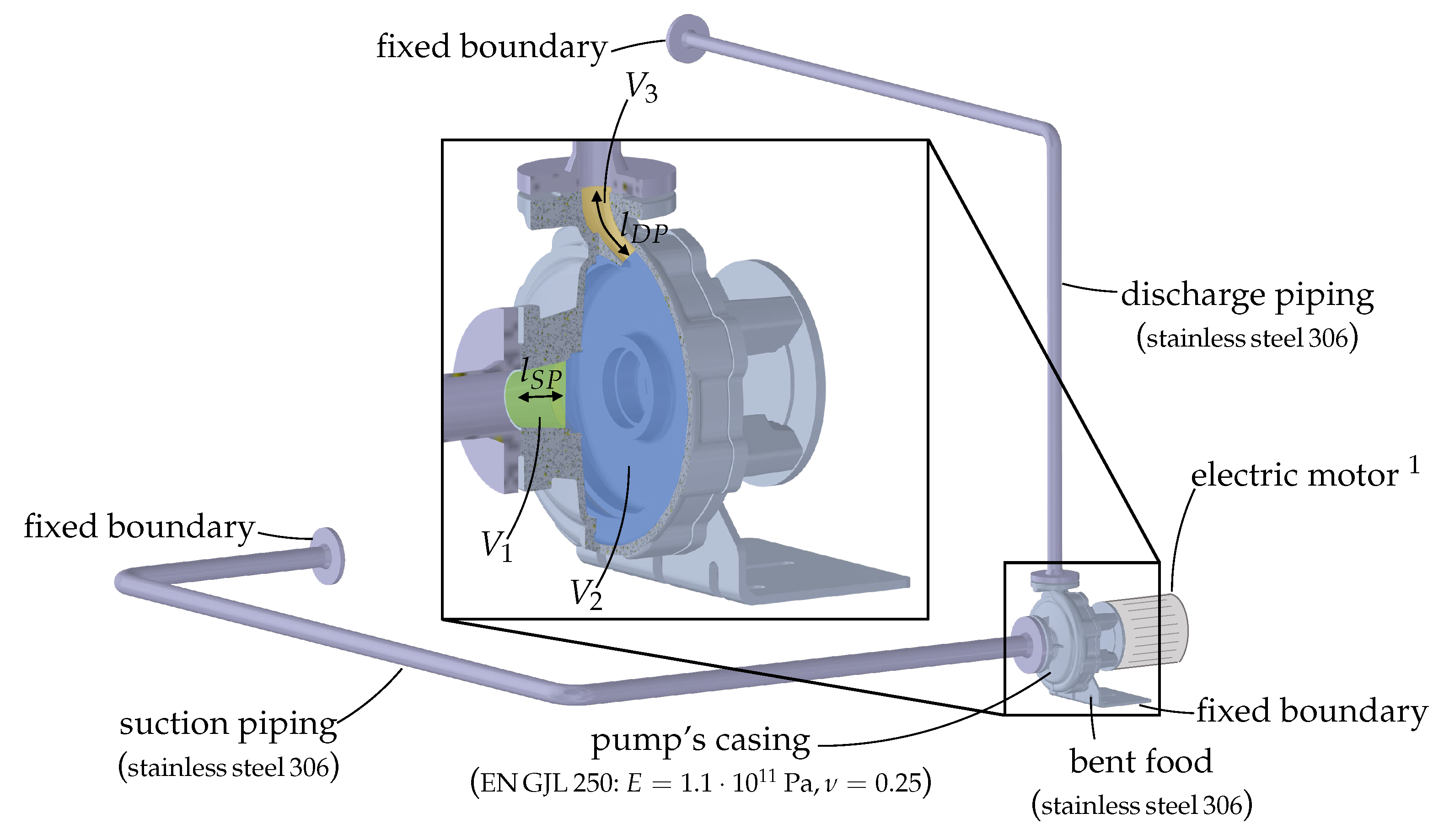
Ansys Mechanical 2023R1) is used to prepare the model, perform the simulation, and post-process the results. The setup used for the FEM is depicted in
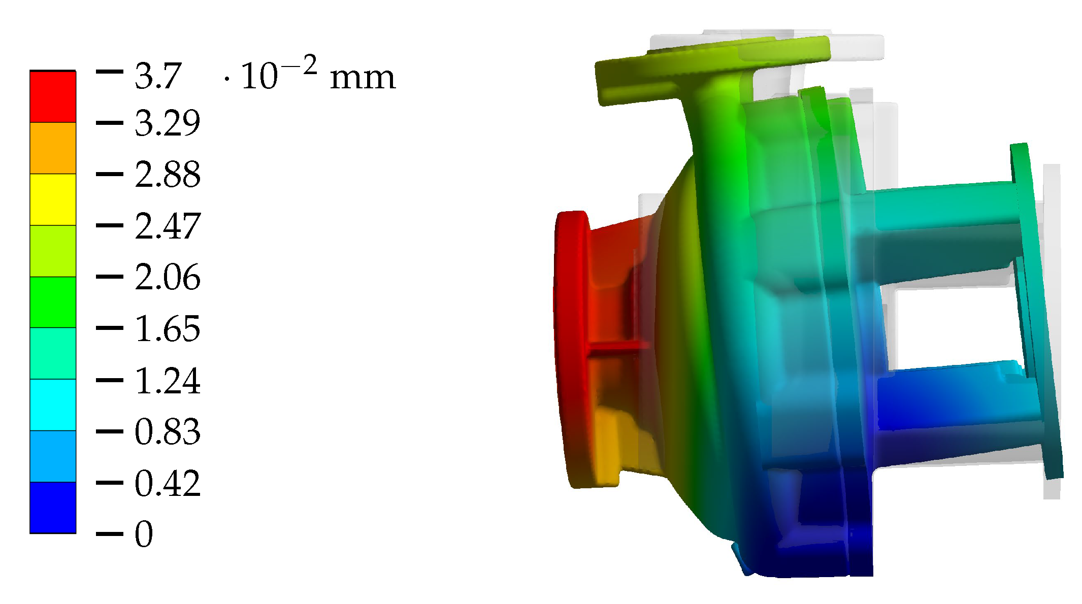
 Figure 4.
The rotor (impeller, shaft, and mechanical seal) and electric motor are not considered for simplification. The pump is connected to a simplified piping system. The flanges of the piping system and the bent foot of the pump are fixed by boundary conditions. The contact elements between the respective bodies are handled as bonded. No gravity is taken into account. According to experiments, the components’ materials are chosen. The stainless steel is of type 306 ( ν = 0.3 , Young’s modulus = 1.95 × 10 11 Pa ). The Young’s modulus of cast iron EN GJL 250 is set to 1.1 × 10 11 Pa and, therefore, to a mean value within the range of manufacturer’s specifications. The native Ansys Mechanical mesh generator is used. The overall element size is prescribed as 10 mm . An additional refinement to 5 mm element size for the pump’s casing is considered. The calculated mesh has about 444,000 tetrahedral elements with quadratic shape functions. To effect a linear elastic deformation of the casing and, therefore, a measurable volume change, the fluid pressure in the pump is varied up to one bar gauge pressure. The total differentials are d V and d p (according to Equation (14)), and so d V d p can be linearised to Δ V Δ p within this range of inner pressure load (this assumption was checked and confirmed within the relevant range of gauge pressure 0 < p 1 bar ). The resulting total displacements of the pump’s casing due to a change in fluid pressure of Δ p = 1 bar are illustrated in Figure 5. The two main causes of displacements are a tilting movement around the pump’s foot and a deformation of the casing, mainly in the areas of the sloping walls between the suction port and spiral contour. The effective speed of sound is influenced in particular by the last mentioned deformation of the casing.
To evaluate the necessary parameters V and Δ V from the FEM results, the fluid volumes V 1 , V 2 , and V 3 within the pump are determined in the undeformed (index 0) and deformed (index Δ p ) cases. In both cases, it is important to use the discretized model to avoid the influence of discretization errors on the target parameters. This kind of error would have a great impact since Δ V is small and of a similar order of magnitude. The values of V 0 and V Δ p for the middle part (volume 2) are both reduced by the rotor’s volume V r o t o r = V i m p e l l e r + V s h a f t + V s e a l . Thus, the rotor neglected for the FEM can be considered again for the calculation of a e f f . However, the compressibility of the rotor, which is made out of cast iron, is disregarded. This simplification is legitimate since the compressibility of cast iron is K 76.4 GPa , which is almost 35 times higher compared to water ( K 2.2 GPa ). The volume change Δ V for all volume parts is calculated by means of Δ V = V Δ p V 0 . The resulting parameters are listed in Table 3. The largest Δ V due to Δ p = 1 bar is calculated for volume 2. The value of Δ V 517 m m 3 is comparable to the volume of an averaged-sized rain drop and seems, thus, rather small compared to V 0 . However, the effective speed of sound is significantly reduced to a e f f = 607 m s 1 , and thus, the effect of the resulting additional compliance is very high. The pump’s suction and discharge ports are stiffer. Δ V even becomes negative in volume 3, which leads to an effective speed of sound which is higher compared to a f = 1482 m s 1 .
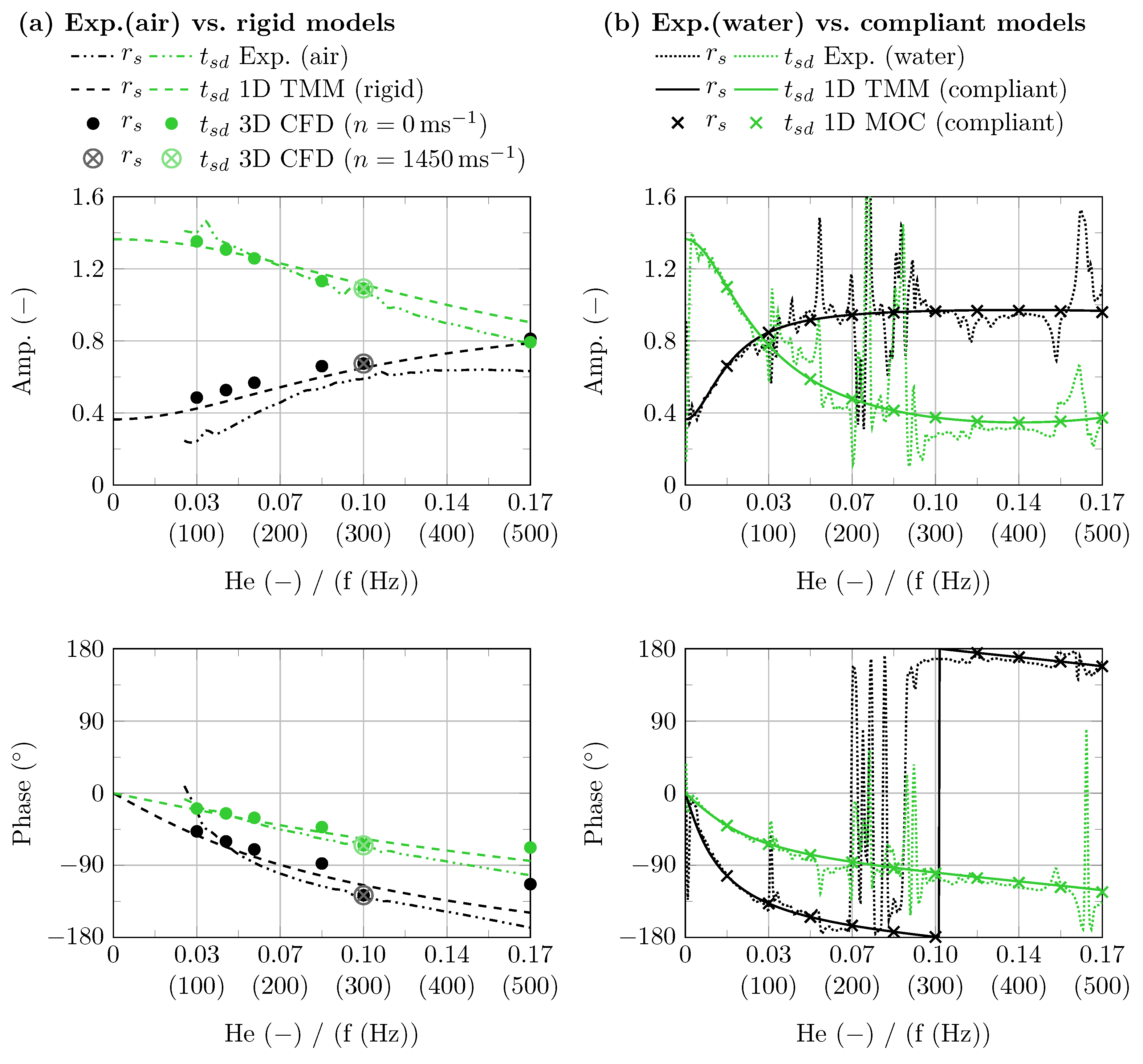
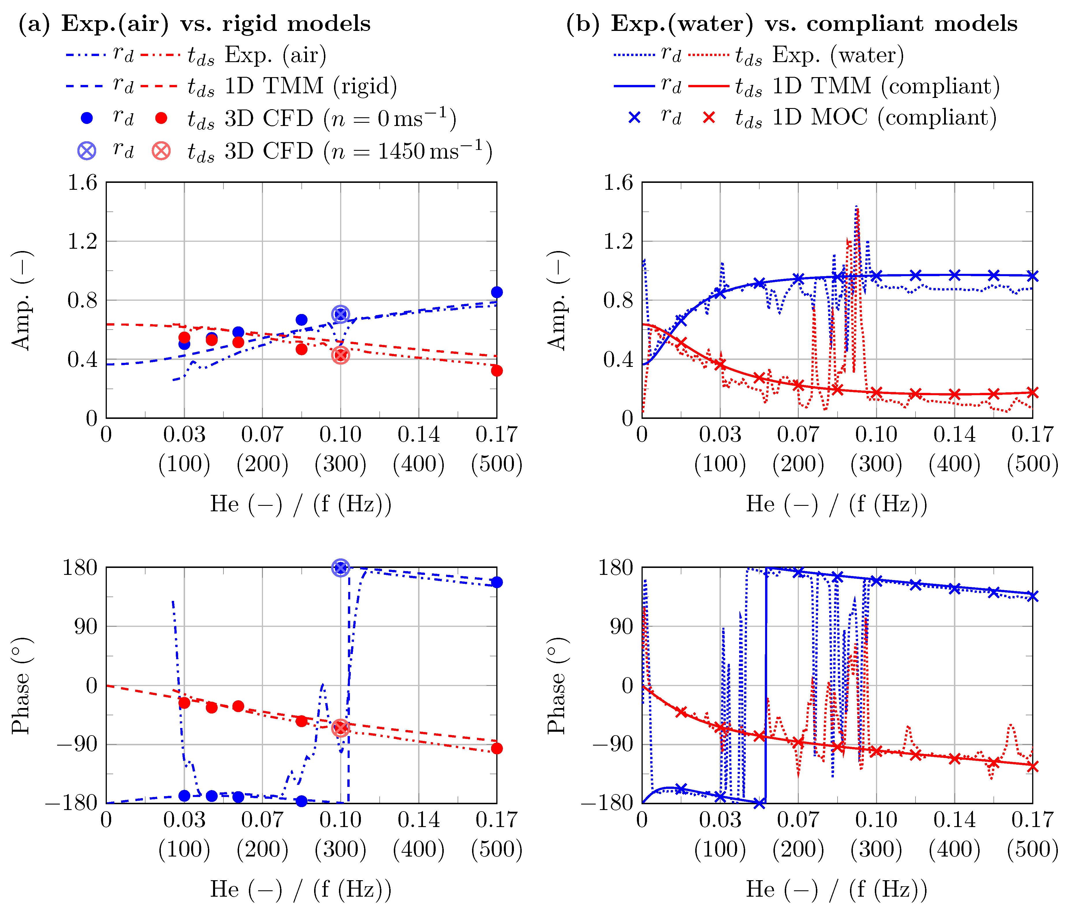
The resulting parameters for the compliant 1D model are listed in Table 4. The transmission coefficients of a rigid model that is geometrically similar to the compliant one are calculated as well. In this case, no additional compliances are considered and, therefore, the speed of sound within the 1D elements equates to the speed of sound in water a e f f = a f = 1482 m s 1 . The wave propagation within the 1D pump model is assumed to be lossless.
The transmission parameters of the compliant model are calculated according to the two-source method based on time-domain simulations by means of the MOC in-house solver FLOAT, as described by [9]. Since only harmonic wave propagation is considered, it is possible to calculate the model’s acoustic transmission behaviour based on the transfer matrix method (TMM) in the frequency domain as well [22]. The transfer matrix T ̲ ̲ p q , e l . for one element (el.) of constant area A connects the sound pressure p ^ ̲ and the sound flux q ^ ̲ = A c ^ ̲ at the element’s inlet and outlet, and is defined as
p ^ ̲ q ^ ̲ d , e l . = c o s ( k l ) i z A s i n ( k l ) i A z s i n ( k l ) c o s ( k l ) T ̲ ̲ p q , e l . p ^ ̲ q ^ ̲ s , e l .
As lossless wave propagation is considered, the wave number k is calculated as a function of frequency f and the effective speed of sound in the respective element a e f f , e l . :
k = 2 π f a e f f , e l .
The specific acoustic impedance is also a function of a e f f , e l . :
z = ρ f a e f f , e l .
Multiplication of the elementary transfer matrices gives the whole model’s functional T ̲ ̲ p q :
T ̲ ̲ p q = T ̲ ̲ p q , p i p e ( d ) × T ̲ ̲ p q , D P × T ̲ ̲ p q , C H × T ̲ ̲ p q , S P × T ̲ ̲ p q , p i p e ( s )
Finally, a change in the acoustic variables from p ^ ̲ and q ^ ̲ to f ^ ̲ and g ^ ̲ is needed to obtain the transmission parameters in the form of the scattering matrix S ̲ ̲ f g . The necessary conversion rules can be found in [23]. Note that the lengths for pipes (s) and (d) are set to a negligible value of 1 mm to consider the cross-section jumps between piping and pump ports within the TMM calculations.

3. Results and Discussion

In Figure 6, the pump’s characteristic head curves evaluated from experiments and 3D CFD simulations for two different rotational speeds are shown. The head h is calculated by means of averaged steady-state values of pressure p and velocity c near the pump’s suction and discharge flanges. The simulated head is higher compared to the experimental results. One reason is the inaccurate reproduction of flow separation at the volute’s tongue due to the use of wall functions. A second reason could be the neglect of surface roughness.
According to [19,20], both simplifications could lead to less pressure loss and, therefore, to an over-prediction of head, which increases with flow rate. However, these possible sources of errors are known and accepted within the scope of this investigation.
In Figure 7, the amplitudes and phases of the transmission parameters related to the pump’s suction side r ^ ̲ s and t ^ ̲ s d determined from experiments (water and air), 3D CFD, and 1D simulations as functions of Helmholtz number H e = f · l a are depicted. As the characteristic length l, the pump’s total acoustic length l = l S P + l C H + l D P = 507 mm is inserted. For the experiments in air, a = 343 m s 1 is used to determine H e . All cases with water are scaled according to a = 1482 m s 1 . The corresponding frequencies f for water are displayed in brackets below the abscissa. The parameters r ^ ̲ d and t ^ ̲ d s related to the pumps pressure side are separately shown in Figure A1 for the benefit of better readability. However, the statements and conclusions made below are the same for both figures. Starting with the configurations declared as rigid (Figure 7a), it can be seen that for both amplitudes and phases the match between 3D CFD, experiments in air, and the 1D TMM model is good. This indicates that the geometric approximation of the 1D approach is valid and sufficient in the requested range of frequencies. Regarding the 3D CFD model, it was further checked if a rotating impeller affects the transmission parameters. Therefore, the nominal operation point at n = 1450 m i n 1 was chosen as an example. Since sound generation at the blade-passing frequency is f 169 Hz in this case, the pump was treated with a sound of f 300 Hz from external sources to determine the transmission parameters. This is performed as usual by means of Equation (7) under the assumption that no pump internal sound sources exist at f 300 Hz . The results clearly indicate that the rotating impeller is not affecting the pump’s passive transmission behaviour. Two statements can be derived from this. Firstly, the assumption that the transmission behaviour of the stationary pump corresponds to that in operation can also be confirmed within the framework of 3D CFD simulations. Secondly, it can be deduced that the numerical interface between the rotating impeller and the stationary mesh parts (“sliding mesh”) does not cause any significant reflections and, therefore, has no influence on the sound transmission.
If the rigid and compliant configurations (Figure 7b) are compared, there is a similar trend for the amplitudes of reflection to increase with higher H e and the reverse trend for the amplitudes of transmission. However, the decisive difference lies in the initial gradients of rigid and compliant cases in a range of 0 < H e 0.07 . Due to the abrupt change in acoustic impedance caused by the compliant casing, incoming sound waves are much more strongly reflected compared to the rigid case. This statement is underlined with respect to the very good approximation of the experiments in water by the 1D TMM and likewise the 1D MOC (compliant) calculations. Nevertheless, it can be seen that the curves determined from experiments in water (Figure 7b) show partly erratic deflections which are not reproduced by the 1D model. It is assumed that this is caused by structural resonances of the entire system, consisting of pump, pipelines, tank, and other attachments. To summarise, this first part of the analysis conducted comparative analyses between rigid simulations and air-based experiments, as well as compliant simulations and water-based experiments, in order to isolate the effect of the fluid–structure interaction on the pump’s acoustic transmission characteristics. The results clearly prove the influence of a reduced effective speed of sound as a result of the casing’s structural compliance on the phase and magnitude of the transmission parameters in the frequency range of interest.
In the next step, the acoustic power ratio ζ , evaluated from the transmission parameters (Equation (8)) for experiments, 3D CFD, and 1D simulations is discussed based on Figure 8. As expected, the results for the 1D models are exactly one. Due to numerical diffusion, the power ratio based on the 3D CFD parameters differs slightly from one as a function of frequency. At 111 Hz , 1.6 % , and at 169 Hz , 2.2 % of the incoming acoustic power dissipates due to the chosen local and temporal discretization (see CFL numbers in Section 2.3). This numerical error is accepted. The experimental values for ζ measured in water and air are both functions of frequency. While the curve calculated from the experimental transmission parameters in water is partly disrupted and unsteady, the one from the experiments in air is smoother. This may be due to the differing influence of the FSI. Apart from this major difference, the trends in both curves are comparably decreasing. This could be coincidental, as the reasons are probably completely different in nature. It is assumed that one main damping effect in water actually comes from friction in mechanical joints [24]. Relative motion between mechanical parts is excited by the strong coupling between the fluid and the structure. In this sense, acoustic power is transmitted from fluid to structure and partially dissipated in non-usable thermal power. The same is unlikely for air, where the FSI influences are much less present. In this case, it is rather to be suspected that thermo-viscous effects in the acoustic boundary layer at structural surfaces within the pump lead to a measurable dissipation of acoustic energy. To compare the orders of magnitude, a size estimation of ζ in water and air due to the acoustic boundary layer is performed in the following. In the textbook [25], an analytical solution for the attenuation coefficient α due to the thermo-viscous boundary layer in a wide cylindrical tube is given (within the framework of boundary layer theory, tubes are declared as wide when their diameter is much larger than the boundary layer thickness [25]). If attenuation is considered, the wave number k becomes
k = 2 π f a + ( 1 + i ) α
The actual geometry of the pump is complex and three-dimensional. In order to, nevertheless, obtain a rough comparison of the size of ζ in water and air, a simple tube with a diameter of d = 17 mm and a length corresponding to the pump’s total acoustic length l = 507 mm is used. Thus, the tube’s inner surface coincides with the middle streamline surface of one single blade channel which is, apart from gaps, the narrowest geometry within the pump. This estimation is to some extent the worst case with respect to the influence of the thermo-viscous acoustic boundary layers, but does not take into account the additional dissipation due to cross-section jumps within the pump. By using Equation (A17) and the quantities given in Appendix B, α is calculated as a function of frequency for water and air. The transfer matrix parameters of the damped tube are calculated by means of Equations (15) and (19) for each medium. The resulting frequency-dependent transfer matrices T ̲ ̲ p q are transformed to scattering matrices S ̲ ̲ f g to calculate the ζ -functions by means of Equation (8). It is found that the minimum values of ζ (at largest H e = 0.17 ) in air are 0.96 and in water 0.99. This little excursus demonstrates that acoustic damping due to thermo-viscous effects is measurable in air and probably negligible in water within the frequency range of interest. Returning to ζ for experiments in water, it is striking that ζ becomes partially greater than one. This type of event seems to occur due to mechanical resonances. According to the definition of ζ , a value greater than one is synonymous with a generation of acoustic energy within the four-pole. Since the pump is at standstill, no fluid dynamic sources should exist. One possible explanation is again the coupling between fluid and structure. In this case, the sound energy would be transferred from the mechanical structures back to the liquid. In order to check this assumption, the power ratio should be extended in future studies to include mechanical–acoustic power components, as, for example, carried our in [1] for simple piping.
In a last step of this study, the source parameters evaluated from the experiments and 3D CFD simulations are analysed and compared. The up- and downstream-propagating source waves f ^ ̲ s r c . and g ^ ̲ s r c . resulting from Equation (1) are further transformed in monopole and dipole amplitudes p ^ ̲ s r c . and c ^ ̲ s r c . by means of Equations (9) and (10). It is important to note that for the transformation of f ^ ̲ s r c . and g ^ ̲ s r c . to a corresponding dipole amplitude, the acoustic impedance in the source region z s r c . is needed. While the acoustic impedance in the whole 3D CFD domain is uniform, it was shown based on the 1D model discussed earlier that the impedance in the experimental pump is significantly changed compared to the pipe. Even if the source determined by means of four-pole theory is located at the discharge flange, the source impedance is calculated based on a e f f , s r c . = 607 m s 1 because the actual dipole source is assumed to be around the volute’s tongue. Based on the static-mechanical FEM simulations (see Section 2.4), it could be shown that deformations of the casing are greatest in this region. In order to obtain dimensionless amplitudes of the monopole and dipole, they are uniformly normalised by means of the circumferential speed at the impeller outlet u 2 and a f = 1482 m s 1 as follows:
p ^ ̲ s r c . , n = p ^ ̲ s r c . 0.5 ρ f u 2 2
c ^ ̲ s r c . , n = c ^ ̲ s r c . × z f 0.5 ρ f u 2 2 with z f = ρ f a f
In Figure 9, the amplitudes of the normalised source term parameters are shown as functions of the relative flow rate for experiments and 3D CFD simulations in a non- and partly reflecting system (NR and CSJ). It can be stated that, especially for the dipole amplitudes, the agreement between simulations and experiments is good. The monopole amplitudes are in the same order of magnitude but the deviations are generally stronger. Due to the normalisation, the dipole amplitudes for different rotational speeds lie close together. The curves of the dipole amplitudes show, for both experiments and simulations, a characteristic increasing trend for part- and overload. The discernible differences between the simulations and measurements are believed to be caused by the neglected influence of the FSI and surface roughness as well as the simplified reproduction of flow separation at the volute’s tongue due to the use of wall functions. The variation in the system impedance (NR and CSJ) has only a negligible influence on the amplitudes of the monopole and dipole. It can be concluded from simulations that the influence of the system’s acoustic impedance on the source mechanisms at the blade-passing frequency is probably small.

4. Conclusions

Based on a combined experimental–numerical approach, it can be shown that the acoustic characteristics of a single-stage centrifugal pump with a volute casing is significantly influenced by fluid–structure interaction. With the help of a 1D model approach, the effective speed of sound within the pump’s casing can be identified as a e f f , c h = 607 m s 1 . The strong reduction in the effective speed of sound leads to an abrupt change in the acoustic impedance. This causes significantly higher sound wave reflections compared to rigid 3D CFD simulations. If the acoustic impedance is further used to evaluate the acoustic dipole source from measurements, the results show good agreement with 3D CFD simulations. Moreover, the system impedance was varied for several 3D CFD simulated operation points. The results indicate that the influence of the system’s impedance on the source mechanisms at the blade-passing frequency is small and predominantly negligible.
Future studies should provide a deeper understanding of the physical causes of pulsation excitation at the blade-passing frequency and how it is linked to the one-dimensional monopole and dipole sources. Another open question is what physical mechanisms lead to a measurable attenuation of sound power in centrifugal pumps. Furthermore, the influence of cavitation on the acoustics of centrifugal pumps should be taken into account. In particular, the knowledge about the acoustic properties of cavitating pumps at the blade-passing frequency seems to be limited. It is, therefore, planned to transfer the presented method to cavitating pumps.

Supplementary Materials

The corresponding data tables for Figure 6, Figure 7, Figure 8 and Figure 9 (Supplementary Files S1–S24) and Figure A1 can be downloaded at: https://www.mdpi.com/article/10.3390/ijtpp9010008/s1.

Author Contributions

Conceptualisation, methodology, project administration, validation, A.B., C.L., P.M. and R.S.; funding acquisition, resources, supervision, A.B. and R.S.; software, formal analysis, investigation, visualisation, C.L. and P.M.; writing—original draft, C.L.; writing—review and editing, A.B., P.M. and R.S. All authors have read and agreed to the published version of the manuscript.

Funding

The presented results were obtained within the research project “Hydroakustik in Kreiselpumpensystemen”. The authors wish to gratefully acknowledge the financial support by the Verband Deutscher Maschinen- und Anlagenbau e.V. (VDMA). Grant number: FKM-Nr. 7051620.

Institutional Review Board Statement

Not applicable.

Informed Consent Statement

Not applicable.

Data Availability Statement

Data is included in the article and the corresponding data tables for the figures can be downloaded as Supplementary Files.

Acknowledgments

We would like to thank Artem Tukalov and Elias Borowski for technical support in the experiments and Jan Phillip Detke, who provided significant support for the evaluations and analyses.

Conflicts of Interest

The authors declare no conflicts of interest.

5. Nomenclature and Abbreviations

The following nomenclature is used in this manuscript:
aSpeed of sound m s 1
ACross-sectional area m 2
cMean velocity m s 1
c p Specific heat at constant pressure J k g 1 K 1
c ^ ̲ Sound particle velocity (complex amplitude) m s 1
dDiameter m
EYoung’s modulus P a
fFrequency H z
f ^ ̲ Downstream pressure wave (complex amplitude) P a
gGravitational acceleration m s 2
g ^ ̲ Upstream pressure wave (complex amplitude) P a
hDischarge head m
H e Helmholtz number
kWave number m 1
lLength m
LPerimeter m
nRotational speed m i n 1
pMean pressure P a
p ^ ̲ Sound pressure (complex amplitude) P a
q r e l Relative flow rate
q ^ ̲ Sound flux (complex amplitude) m 3 s 1
Q ˙ Flow rate m 3 h 1
r ^ ̲ Sound reflection parameter (complex amplitude)
sWall thickness m
S ̲ ̲ Scattering matrix
tTime s
t ^ ̲ Sound transmission parameter (complex amplitude)
TTemperature K
T ̲ ̲ Transfer matrix
uCircumferential speed m s 1
VFluid volume m 3
xLocal coordinate relative to the pump’s flanges m
y + Dimensionless wall distance
zSpecific acoustic impedance k g m 2 s 1
ZAcoustic impedance k g m 4 s 1
α Attenuation coefficient m 1
γ Ratio of specific heats
ϵ Relative error%
ζ Acoustic power ratio
κ Thermal conductivity W m 1 K 1
λ Acoustic wave length m
μ Dynamic viscosity k g m 1 s 1
ν Poisson’s ratio
ρ Mean density k g m 3
The following abbreviations are used in this manuscript:
Amp.Amplitude
BCBoundary condition
BPBlade-passing
CFDComputational fluid dynamics
CHChannel
compl.Compliant
CSJCross-section jump
DFTDiscrete Fourier transformation
DPDischarge port
EOSEquation of state
FEMFinite element method
FDFinite difference
FSIFluid–structure interaction
FVFinite volume
IFInterface
MOCMethod of characteristics
no.Number of
NRBCNon-reflective boundary condition
opt.Optional
PEPiezoelectric
URANSUnsteady Reynolds-averaged Navier–Stokes
RSIRotor–stator interaction
SIMPLESemi-implicit method for pressure linked equations
SPSuction port
src.Source
SSTShear stress transport
TMMTransfer matrix method
1DOne-dimensional
3DThree-dimensional
The following indices are used in this manuscript:
acAcoustic
dDischarge
CHChamber
DPDischarge port
effEffective
el.Element
fFluid
nNormalised
NNominal
pPump
sSuction
SPSuction port
relRelative
src.Source
sys(piping) System (connected to the pump)
tTube
0Undeformed
ΔpDeformed

Appendix A

The power ratio ζ of a four-pole can be calculated by means of the ratio of outgoing and incoming time-averaged acoustic powers P ¯ o u t and P ¯ i n (see Equation (8)). Since the pump’s transfer function is represented as a scattering matrix, it is useful to find formulations for P ¯ o u t and P ¯ i n as functions of outgoing ( g ^ ̲ s , f ^ ̲ d ) and incoming pressure waves ( f ^ ̲ s , g ^ ̲ d ), respectively. The time-averaged acoustic power at a specific location x in a tube can be calculated by means of the following relation [26]:
P ¯ = 1 2 A t p ^ ( x ) c ^ ( x )
A t is the internal cross-sectional area of the pipe; p ^ ( x ) and c ^ ( x ) are the amplitudes of the pressure and sound particle velocity. If Equation (A1) is extended by
p ^ = | f ^ ̲ e i k x + g ^ ̲ e i k x |
and
c ^ = | f ^ ̲ e i k x g ^ ̲ e i k x | 1 ρ f a e f f , t
at x = 0 , it follows that
P ¯ = 1 2 Z t | f ^ ̲ 2 g ^ ̲ 2 | .
Herein, Z t is the acoustic impedance within the pipe and is generally defined as follows:
Z t = ρ f a e f f , t A t
where ρ f is the density of the fluid. If Equation (A4) is applied to the pump’s suction and discharge ports and further split into parts of power going in and out of the four-pole (since the power components associated with f ^ ̲ and g ^ ̲ are split in the next step, the absolute value function in | f ^ ̲ 2 g ^ ̲ 2 | is applied separately to subtrahend and minuend: | ^ ̲ 2 | = ^ 2 ), it results in
P ¯ i n = 1 2 Z t , s f ^ s 2 + 1 2 Z t , d g ^ d 2
and
P ¯ o u t = 1 2 Z t , s g ^ s 2 + 1 2 Z t , d f ^ d 2 .
The acoustic power ratio ζ of P ¯ o u t and P ¯ i n can, therefore, be calculated as a function of outgoing ( g ^ ̲ s , f ^ ̲ d ) and incoming ( f ^ ̲ s , g ^ ̲ d ) pressure waves:
ζ = Z t , d Z t , s g ^ s 2 + f ^ d 2 Z t , d Z t , s f ^ s 2 + g ^ d 2 .
Furthermore, a formulation for ζ as a function of the transmission parameters is to be developed. If the acoustic source parameters in the pump are assumed to be zero, Equation (1) simplifies to
f ^ ̲ d g ^ ̲ s = t ^ ̲ s d r ^ ̲ d r ^ ̲ s t ^ ̲ d s S ̲ ̲ f g f ^ ̲ s g ^ ̲ d
It is possible to analyse the scattering of the incoming pressure waves and their acoustic power separately [23]. For f ^ s this is achieved by setting g ^ d = 0 . It follows from Equation (A6)
P ¯ i n , f s = 1 2 Z t , s f ^ s 2 ,
and from Equation (A9) for the absolute values of
g ^ s = r ^ s f ^ s
as well as
f ^ d = t ^ s d f ^ s
Substituting Equations (A11) and (A12) into Equation (A7) gives
P ¯ o u t , f s = 1 2 Z t , s r ^ s 2 f ^ s 2 + 1 2 Z t , d t ^ s d 2 f ^ s 2
By means of Equations (A10) and (A13) the power ratio ζ f s (i.e., for g ^ d = 0 ) can be determined by
ζ f s = P ¯ o u t , f s P ¯ i n , f s = r ^ s 2 + Z t , s Z t , d t ^ s d 2
In order to evaluate ζ g d , the analogue procedure by setting f ^ s = 0 gives
ζ g d = P ¯ o u t , g d P ¯ i n , g d = r ^ d 2 + Z t , d Z t , s t ^ d s 2
Finally, the power ratio of the four-pole ζ can be determined by the mean value of the two power ratios ζ f s and ζ g d and, therefore, as a function of the pump’s transmission parameters:
ζ = ζ f s + ζ g d 2 = r ^ s 2 + Z t , s Z t , d t ^ s d 2 + r ^ d 2 + Z t , d Z t , s t ^ d s 2 2 .

Appendix B

The attenuation of sound in wide cylindrical tubes due to the effect of a thermo-viscous boundary layer can be calculated by means of the following equation given by [25]:
α = 2 3 / 2 2 π f μ ρ a 2 1 / 2 1 + γ 1 ( Pr ) 1 / 2 L A ,
where μ , γ , and Pr are the fluid specific dynamic viscosity, the ratio of specific heats and the Prandtl number. The latter is defined as
Pr = μ c p κ
κ and c p are the thermal conductivity and the specific heat at constant pressure. L and A are the inner perimeter and cross-sectional area of the tube. The speed of sound in air is assumed to be a = 343 m s 1 . For water, the lowest effective speed of sound in the pump is used, a = a e f f = 607 m s 1 . The remaining quantities used to calculate α in a water- or air-filled tube at ambient conditions ( T = 20 ° , atmospheric pressure) are listed in Table A1.
Table A1. Quantities used to determine α at ambient conditions ( T = 20 ° , atmospheric pressure), taken from [25].
ParameterUnitAirWater
μ k g m 1 s 1 18.2 × 10 6 1.002 × 10 3
γ 1.41
κ W m 1 K 1 0.06260.597
c p J k g 1 K 1 1.005 × 10 3 4.18 × 10 3
Figure A1. Amplitude and phase of transmission parameters r ^ ̲ d and t ^ ̲ d s evaluated from experiments (water and air), CFD, and 1D simulations as functions of Helmholtz number. Corresponding frequencies f for water are displayed in brackets below the abscissa. (Data: Supplementary Files S5–S12).
Ijtpp 09 00008 g0a1

References

  1. De Jong, C. Analysis of Pulsations and Vibrations in Fluid-Filled Pipe Systems. Ph.D. Thesis, Eindhoven University of Technologie, Eindhoven, The Netherlands, 1994. [Google Scholar]
  2. Rzentkowski, G.; Zbroja, S. Experimental Characerization of Centrifugal Pumps as an Acoustic Source at the Blade-Passing Frequency. J. Fluids Struct. 2000, 14, 529–558. [Google Scholar] [CrossRef]
  3. Gülich, J. Centrifugal Pumps, 4th ed.; Springer: Berlin/Heidelberg, Germany, 2020. [Google Scholar]
  4. Parrondo, J.; Pérez, J.; Fernández, J. The Effect of the Operation Point on the Pressure Fluctuations at the Blade-Passing Frequency in the Volute of a Centrifugal Pump. J. Fluids Eng. 2002, 124, 784–790. [Google Scholar] [CrossRef]
  5. Grieb, H. Verdichter für Turbo- und Flugtriebwerke; Springer: Berlin/Heidelberg, Germany, 2009. [Google Scholar]
  6. Brennen, C.E. Hydrodynamics of Pumps, 2nd ed.; Cambridge University Press: Cambridge, UK, 2011. [Google Scholar]
  7. Gülich, J.; Bolleter, U. Pressure Pulsations in Centrifugal Pumps. J. Vib. Acoust. 1992, 114, 272–279. [Google Scholar] [CrossRef]
  8. Lehr, C.; Linkamp, A.; Brümmer, A. Druckpulsationen in Instationär Betriebenen Hydraulischen Systemen; Technical Report; TU Dortmund University, Chair of Fluidics: Dortmund, Germany, 2019. [Google Scholar]
  9. Lehr, C.; Linkamp, A.; Aurich, D.; Brümmer, A. Simulations and experimental investigations on the acoustic characterization of centrifugal pumps of different specific speed. Int. J. Turbomach. Propuls. Power 2019, 4, 16. [Google Scholar] [CrossRef]
  10. Johnston, N. High-precision in situ measurement of speed of sound in hydraulic systems. J. Syst. Control. Eng. 2020, 234, 299–313. [Google Scholar] [CrossRef]
  11. Lehr, C.; Munsch, P.; Skoda, R.; Brümmer, A. Numerical and experimental investigations on the acoustic characteristics of a single-stage centrifugal pump. In Proceedings of the European Conference on Turbomachinery Fluid dynamics & Thermodynamics, Budapest, Hungary, 24–28 April 2023; Paper n. ETC2023-325. Available online: https://www.euroturbo.eu/publications/conference-proceedings-repository/etc15-2023/ (accessed on 15 November 2023).
  12. Chung, D.A.; Blaser, J.Y. Transfer function method of measuring in-duct acoustic properties. I. Theory. J. Acoustic Soc. Am. 1980, 68, 907–913. [Google Scholar] [CrossRef]
  13. Horlacher, H.B.; Lüdecke, H.J. Strömungsberechnung für Rohrsysteme, 2nd ed.; Expert Verlag: Renningen, Germany, 2006. [Google Scholar]
  14. Schwarz, H.; Köckler, N. Numerische Mathematik, 8th ed.; Vieweg + Teubner: Wiesbaden, Germany, 2011. [Google Scholar]
  15. Bardeleben, M. Acoustic Characterization of a Centrifugal Pump Using a Two-Port Model. Ph.D. Thesis, McMaster University Hamilton, Hamilton, ON, Canada, 2005. [Google Scholar]
  16. Åbom, M. A Note on the Experimental Determination of Acoustical Two-Port Matrices. J. Sound Vib. 1992, 155, 185–188. [Google Scholar] [CrossRef]
  17. Kiermeier, J. Numerische Simulation einphasiger sowie kavitierender Strömungen in oszillierenden Verdrängerpumpen. Ph.D. Thesis, Technische Universität München, München, Germany, 2015. [Google Scholar]
  18. Munsch, P.; Lehr, C.; Brümmer, A.; Skoda, R. A Compressible, Coupled Three-Dimensional/One-Dimensional Flow Solution Method for the Seamless Simulation of Centrifugal Pumps and Their Piping. J. Fluids Eng. 2023, 145, 091203. [Google Scholar] [CrossRef]
  19. Limbach, P.; Skoda, R. Numerical and experimental analysis of cavitating flow in a low specific speed centrifugal pump with different surface roughness. J. Fluids Eng. 2017, 139, 101201. [Google Scholar] [CrossRef]
  20. Juckelandt, K.; Wurm, F.H. Applicability of Wall-Function Approach in Simulations of Turbomachines. In Proceedings of the ASME Turbo Expo: Turbine Technical Conference and Exposition, Montreal, QB, Canada, 15–19 June 2015. [Google Scholar]
  21. Linkamp, A.; Deimel, C.; Brümmer, A.; Skoda, R. Non-reflecting coupling method for one-dimensional finite difference/finite volume schemes based on spectral error analysis. Comput. Fluids 2016, 140, 334–346. [Google Scholar] [CrossRef]
  22. Munjal, M. Acoustics of Ducts and Mufflers, 2nd ed.; John Wiley & Sons: Hoboken, NJ, USA, 2014. [Google Scholar]
  23. Gentemann, A.M.G. Identifikation von Akustischen Transfermatrizen und Flammenfrequenzgängen Mittels Strömungssimulation. Ph.D. Thesis, Technischen Universität München, München, Germany, 2006. [Google Scholar]
  24. Niehus, K.K. Identifikation linearer Dämpfungsmodelle für Werkzeugmaschinenstrukturen. Ph.D. Thesis, Technische Univeristät München, München, Germany, 2015. [Google Scholar]
  25. Pierce, A.D. Acoustics: An Introduction to Its Physical Principles and Applications, 3rd ed.; Springer: Cham, Switzerland, 2019. [Google Scholar]
  26. Meyer, E.; Neumann, E.G. Physikalische und Technische Akustik; Springer: Wiesbaden, Germany, 1979. [Google Scholar]
Figure 1. Four−pole representation of the pump connected to a piping system.
Ijtpp 09 00008 g001
Figure 2. (a) Closed−circuit centrifugal pump test rig and (b) schematic representation with measurement positions and named components.
Ijtpp 09 00008 g002
Figure 3. Structure of the simulation area with position information on used monitor points (CSJ = cross-section jump, NR = non-reflective boundary condition, IF = interface, src. = source, opt. = optional).
Ijtpp 09 00008 g003
Figure 4. FEM model setup and subdivision of fluid volumes in the pump. 1 Not considered for the simulation.
Ijtpp 09 00008 g004
Figure 5. Total displacements of the pump’s casing calculated by means of static mechanical FEM simulations (the colour code corresponds to the original displacements whereas the moving patterns in the picture are scaled by 1300 × true scale”).
Ijtpp 09 00008 g005
Figure 6. Pump’s characteristic head curves evaluated from experiments and 3D CFD simulations for two different rotational speeds. (Data: Supplementary Files S1–S4).
Ijtpp 09 00008 g006
Figure 7. Amplitude and phase of transmission parameters r ^ ̲ s and t ^ ̲ s d evaluated from experiments (water and air), 3D CFD, and 1D simulations as functions of Helmholtz number. Corresponding frequencies f for water are displayed in brackets below the abscissa. (Data: Supplementary Files S5–S12).
Ijtpp 09 00008 g007
Figure 8. Acoustic power ratio ζ evaluated from transmission parameters for experiments, 3D CFD, and 1D simulations as functions of Helmholtz number H e . (Data: Supplementary Files S13–S18).
Ijtpp 09 00008 g008
Figure 9. Amplitudes of normalised source term parameters for monopole and dipole at blade-passing frequency ( f B P [ 111 ; 169 ] Hz) as functions of the relative flow rate evaluated from experiments and 3D CFD simulations for two different rotational speeds. (Data: Supplementary Files S19–S24).
Ijtpp 09 00008 g009
Table 1. Specifications of the pump under investigation ( n s = specific speed (according to n s = n N Q ˙ N h N 0.75 with n N in m i n 1 , Q ˙ N in m 3 s 1 , and h N in m), d 2 = impeller outlet diameter; abbreviations: N = nominal, no. = number of).
n s ( min 1 ) d 2 ( mm ) d 2 d tongue 2 ( mm ) No. Blades ( ) n N ( min 1 ) h N ( m ) Q ˙ N ( m 3 h 1 ) N P S H 3 % ( m )
122227.5714501515.51.57
Table 2. Sensor positions relative to the pump’s flanges.
Sensor p s 1 p s 2 p s 3 p s 4 p s p d p d 1 p d 2 p d 3 p d 4
Distance Δ x (m)−1.16−0.89−0.57−0.26−0.1450.1750.260.570.891.16
Table 3. Fluid volumes based on the FEM model and resulting a e f f .
ParameterUnitVolume 1Volume 2Volume 3
Δ p ( Pa ) 1 × 10 5 1 × 10 5 1 × 10 5
V 0 ( m m 3 ) 114,648.022,287,892.89 *40,854.596
V Δ p ( m m 3 ) 114,651.322,288,409.65 *40,854.540
Δ V ( m m 3 ) 3.3516.76−0.056
a e f f ( m s 1 ) 11586071500
* Determined by V = V 2 V r o t o r with V 2 from FEM-simulation (with indices 0 for undeformed and Δ p for deformed structure) and V r o t o r = V i m p e l l e r + V s h a f t + V s e a l from the pump’s CAD model. Determined by Δ V = V Δ p V 0 . Determined using Equation (14).
Table 4. 1D model parameters (d, l, and a e f f ) for the pump under investigation.
ParameterUnitPipe (s)SPCHDPPipe (d)
d ( mm ) 54.556862637.2
l ( mm ) 149388701
a e f f ( m s 1 ) 1350115860715001350
Disclaimer/Publisher’s Note: The statements, opinions and data contained in all publications are solely those of the individual author(s) and contributor(s) and not of MDPI and/or the editor(s). MDPI and/or the editor(s) disclaim responsibility for any injury to people or property resulting from any ideas, methods, instructions or products referred to in the content.

