
Low-Noise Airfoils for Turbomachinery Applications: Two Examples of Optimization †


Abstract
1. Introduction
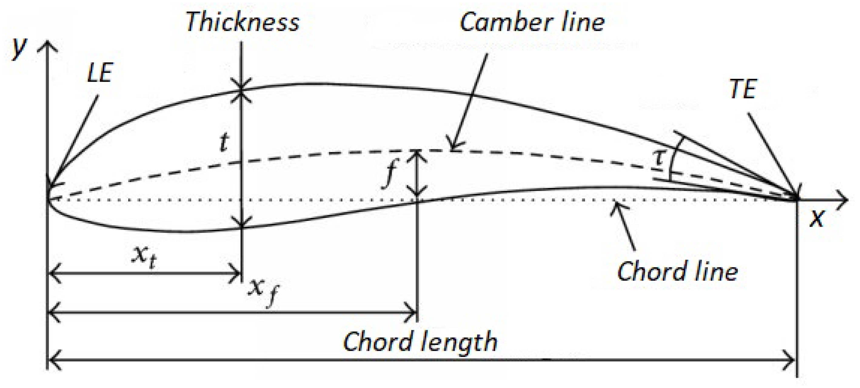
2. Methodology
2.1. Low-Fidelity Approach
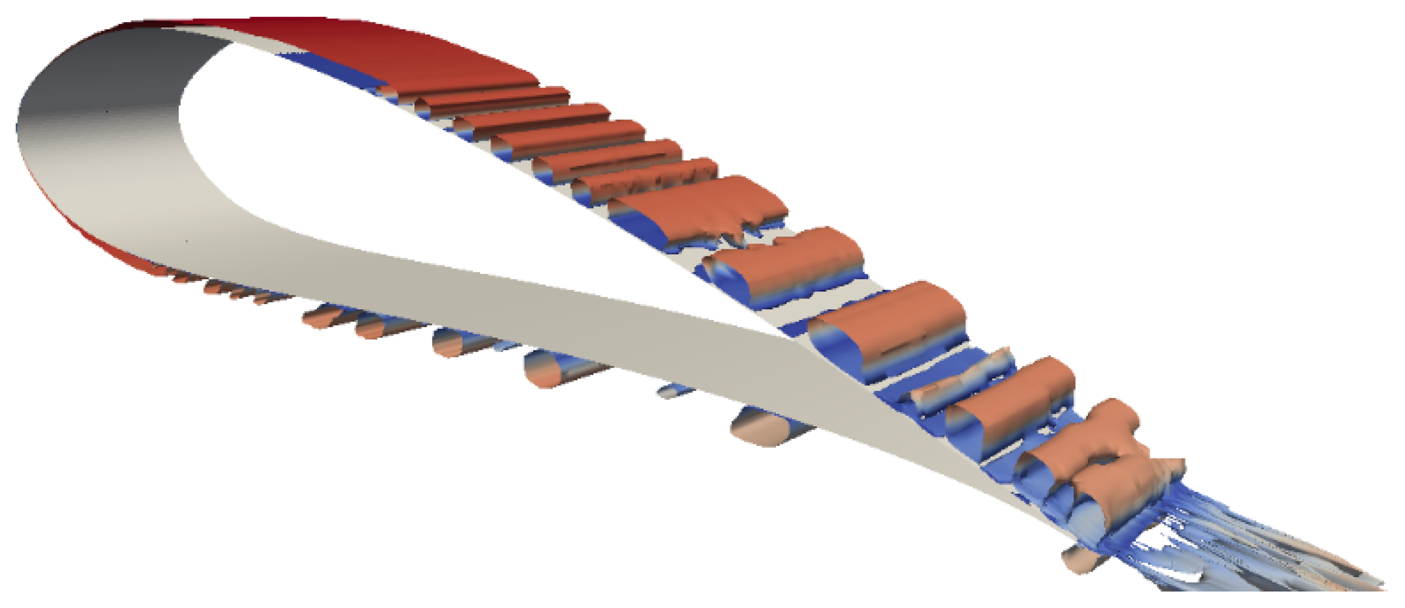
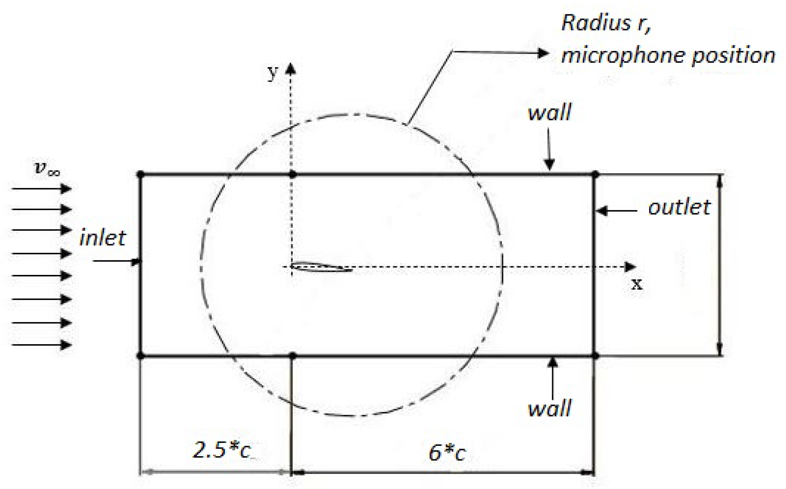
2.2. High-Fidelity Approach
2.3. Optimization
3. Results
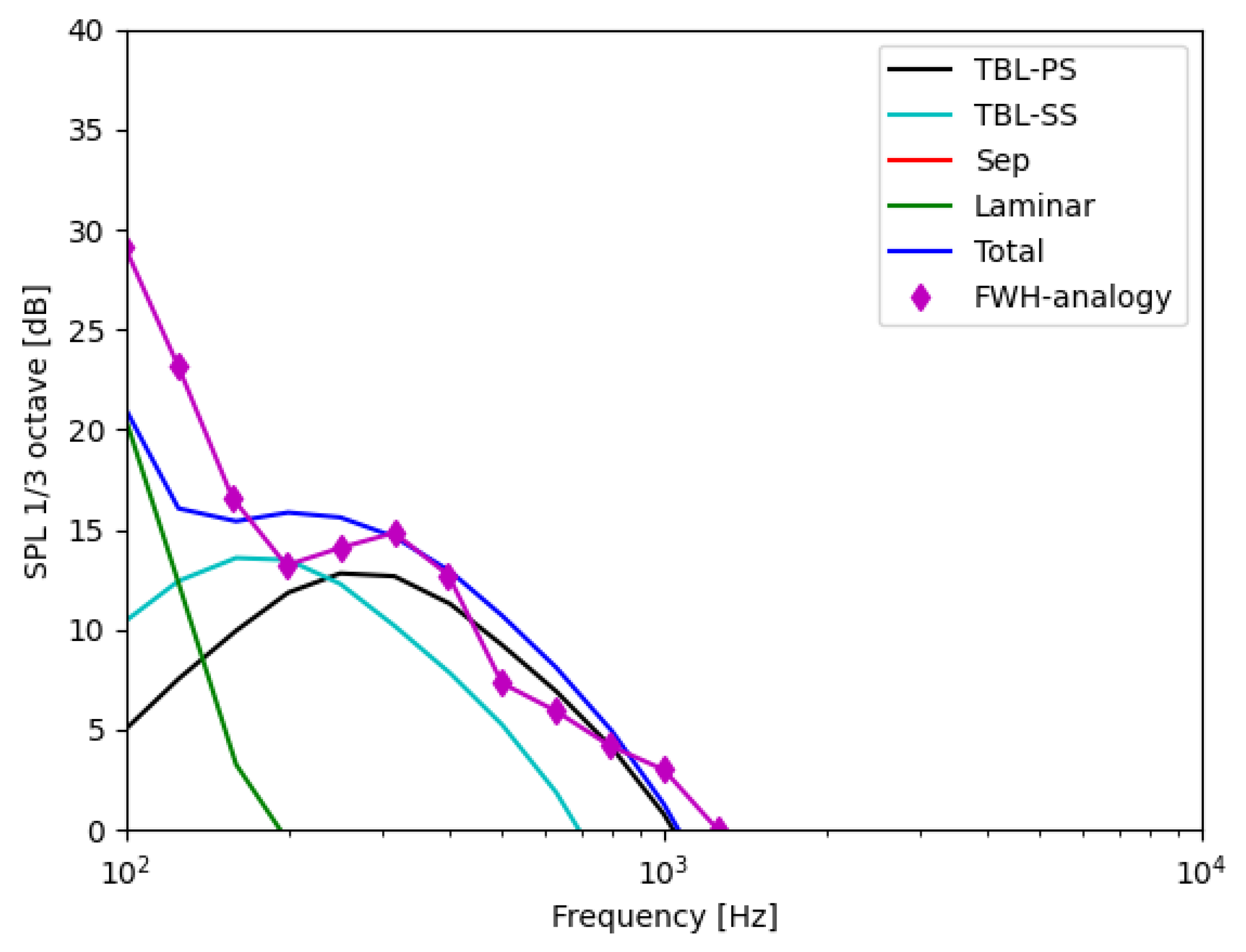
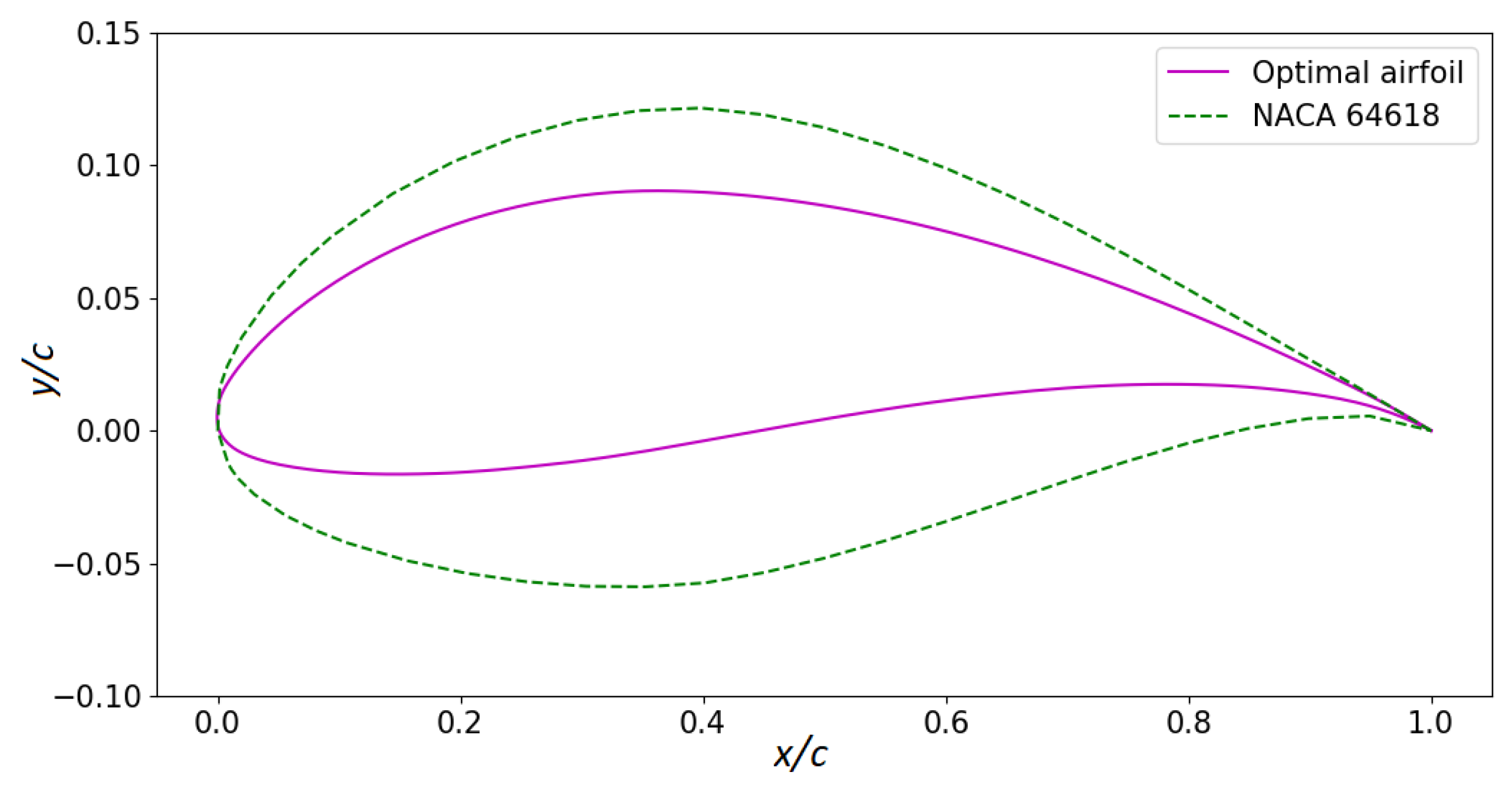
3.1. NACA 64618 Validation Case
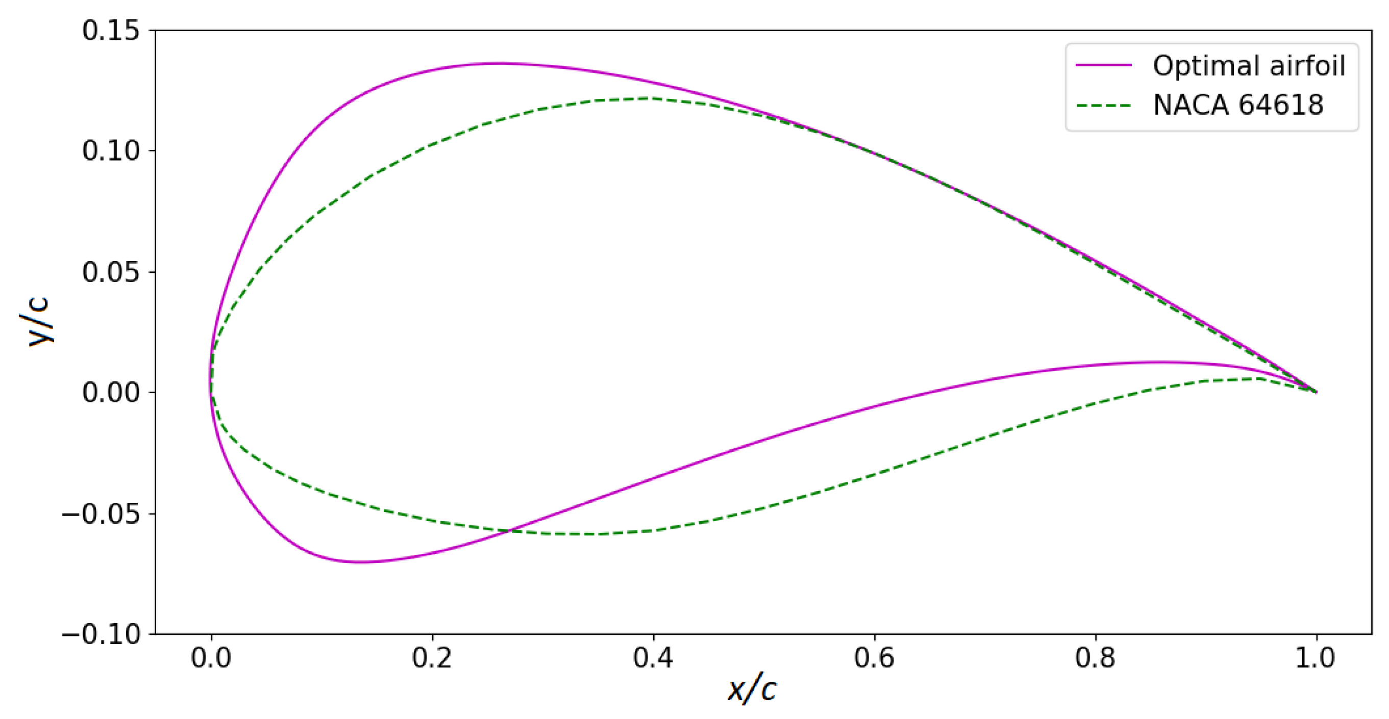
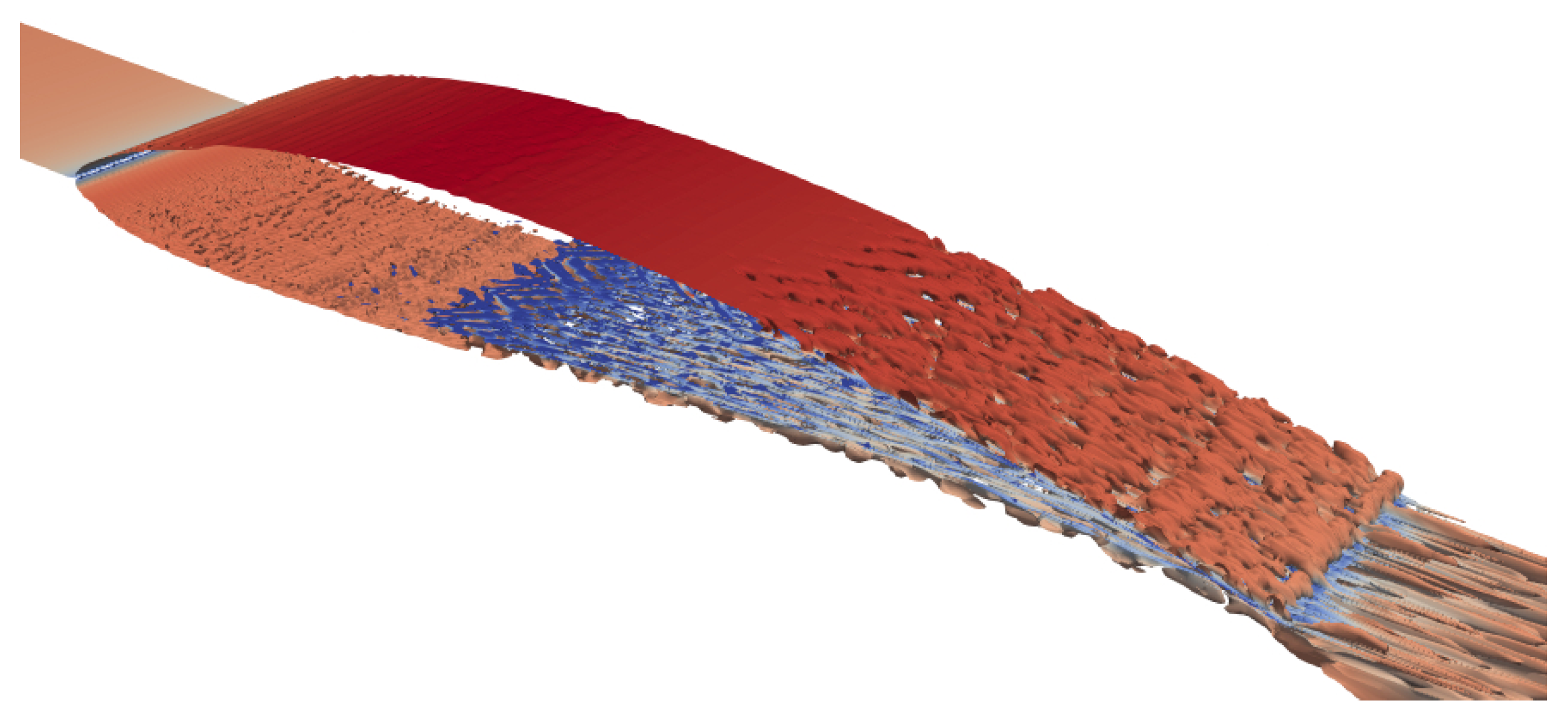
3.2. High-Reynolds Optimization
- Thickness: Both the T-PS and the T-SS contribution had a higher value, and the maximum value was reached for a lower frequency.
- Position of maximum thickness: Similar effects as the thickness contribution—increased noise emissions and shift towards lower frequencies. In this case, increasing the parameters translated into displacing the maximum thickness position towards the TE.
- Maximum camber value: Both T-PS and T-SS contributions had a higher maximum value, but in this case, the frequencies at which these values are reached remain unchanged.
- Position of maximum camber: The same effects as the maximum camber contribution.
3.3. NACA 64618 Low-Reynolds Number Case
3.4. Low-Reynolds Optimization
- Thickness: Both T-PS and T-SS contributions had a higher value, and the maximum value was reached for a lower frequency. Instead, the Laminar contribution had a lower value and the frequency corresponding to the maximum value remains unchanged.
- Position of maximum thickness: Similar effects as the thickness contribution.
- Maximum camber value: The T-PS and T-SS contributions had a higher maximum value, but in this case, the frequencies at which these values were reached remain unchanged. As regards the laminar contribution, it had a lower value, and the frequency corresponding to the maximum value was lower.
- Position of maximum camber: The same effects as the maximum camber contribution.
4. Conclusions
Author Contributions
Funding
Institutional Review Board Statement
Informed Consent Statement
Data Availability Statement
Conflicts of Interest
Abbreviations
| AoA | Angle of Attack |
| BEM | Boundary Element Method |
| BPM | Brooks Pope and Marcolini Method |
| c | Chord |
| CFL | Courant–Friedrichs–Lewy number |
| FWH | Ffowcs Williams Hawkings Analogy |
| LDR | Lift-to-Drag Ratio |
| LE | Leading Edge |
| OSPL | Overall Sound Pressure Level |
| PS | Pressure Side |
| SHG | Simplicial Homology Global |
| SPL | Sound Pressure Level |
| SS | Suction Side |
| TE | Trailing Edge |
References
- Qin, Y.; Tang, X.; Jia, T.; Duan, Z.; Zhang, J.; Li, Y.; Zheng, L. Noise and vibration suppression in hybrid electric vehicles: State of the art and challenges. Renew. Sustain. Energy Rev. 2020, 124, 109782. [Google Scholar] [CrossRef]
- Rogers, A.L.; Manwell, J.F.; Wright, S. Wind turbine acoustic noise. In Renewable Energy Research Laboratory; University of Massachusetts: Amherst, MA, USA, 2006. [Google Scholar]
- Wright, S. The acoustic spectrum of axial flow machines. J. Sound Vib. 1976, 45, 165–223. [Google Scholar] [CrossRef]
- Moreau, S.; Roger, M. Competing broadband noise mechanisms in low-speed axial fans. AIAA J. 2007, 45, 48–57. [Google Scholar] [CrossRef]
- Casari, N.; Fadiga, E.; Oliani, S.; Pinelli, M.; Piovan, M. A Low-Noise Airfoil for Low Reynolds Applications: A Multi-Fidelity Optimization. In Proceedings of the 15th European Turbomachinery Conference, Paper n. ETC2023-181, Budapest, Hungary, 24–28 April 2023; Available online: https://www.euroturbo.eu/publications/proceedings-papers/etc2023-181/ (accessed on 1 July 2023).
- Lacagnina, G.; Chaitanya, P.; Kim, J.H.; Berk, T.; Joseph, P.; Choi, K.S.; Ganapathisubramani, B.; Hasheminejad, S.M.; Chong, T.P.; Stalnov, O.; et al. Leading edge serrations for the reduction of aerofoil self-noise at low angle of attack, pre-stall and post-stall conditions. Int. J. Aeroacoustics 2021, 20, 130–156. [Google Scholar] [CrossRef]
- Zhong, Y.; Li, Y.; Li, P.; Chen, J.; Xia, T.; Kuang, X. Blade Structure Design Based on Multi-objective Optimization of Automotive Fan. In Proceedings of the Journal of Physics: Conference Series; IOP Publishing: Bristol, UK, 2021; Volume 1952, p. 032022. [Google Scholar]
- Ffowcs Williams, J.E.; Hawkings, D.L. Sound generation by turbulence and surfaces in arbitrary motion. Philos. Trans. R. Soc. Lond. Ser. A Math. Phys. Sci. 1969, 264, 321–342. [Google Scholar]
- Brooks, T.F.; Pope, D.S.; Marcolini, M.A. Airfoil Self-Noise and Prediction; NASA Reference Publication 1208; National Technical Information Service: Springfield, VA, USA, 1989. [Google Scholar]
- Shen, W.Z.; Zhu, W.J.; Fischer, A.; García, N.R.; Cheng, J.; Chen, J.; Madsen, J. Validation of the CQU-DTU-LN1 series of airfoils. In Proceedings of the Journal of Physics: Conference Series; IOP Publishing: Bristol, UK, 2014; Volume 555, p. 012093. [Google Scholar]
- Casari, N.; Oliani, S.; Pinelli, M.; Piovan, M.; de Paola, E.; Stoica, L.G.; Marco, A.D.; Mollica, E. Towards a low-noise axial fan for automotive applications. Proc. J. Phys. Conf. Ser. 2022, 2385, 012137. [Google Scholar] [CrossRef]
- Drela, M. XFOIL: An analysis and design system for low Reynolds number airfoils. In Low Reynolds Number Aerodynamics; Springer: Berlin/Heidelberg, Germany, 1989; pp. 1–12. [Google Scholar]
- Nicoud, F.; Ducros, F. Subgrid-scale stress modelling based on the square of the velocity gradient tensor. Flow Turbul. Combust. 1999, 62, 183–200. [Google Scholar] [CrossRef]
- Langtry, R.B.; Menter, F.R. Correlation-based transition modeling for unstructured parallelized computational fluid dynamics codes. AIAA J. 2009, 47, 2894–2906. [Google Scholar] [CrossRef]
- Wagner, C.; Hüttl, T.; Sagaut, P. Large-Eddy Simulation for Acoustics; Cambridge University Press: Cambridge, UK, 2007; Volume 20. [Google Scholar]
- Celik, I.B.; Cehreli, Z.N.; Yavuz, I. Index of Resolution Quality for Large Eddy Simulations. J. Fluids Eng. 2005, 127, 949–958. [Google Scholar] [CrossRef]
- Epikhin, A.; Evdokimov, I.; Kraposhin, M.; Kalugin, M.; Strijhak, S. Development of a dynamic library for computational aeroacoustics applications using the OpenFOAM open source package. Procedia Comput. Sci. 2015, 66, 150–157. [Google Scholar] [CrossRef]
- Liang, Y.; Zhang, L.; Li, E.; Liu, X.; Yang, Y. Design considerations of rotor configuration for straight-bladed vertical axis wind turbines. Adv. Mech. Eng. 2014, 2014, 1–15. [Google Scholar] [CrossRef]
- Abdessemed, C.; Bouferrouk, A.; Yao, Y. Aerodynamic and aeroacoustic analysis of a harmonically morphing airfoil using dynamic meshing. Acoustics 2021, 3, 177–199. [Google Scholar] [CrossRef]
- Jeong, J.; Hussain, F. On the identification of a vortex. J. Fluid Mech. 1995, 285, 69–94. [Google Scholar] [CrossRef]


| Airfoil | AoA | LDR | OSPL | ||
|---|---|---|---|---|---|
| NACA 64618 | −0.268 | 0.52 | 0.0061 | 85.24 | 62.5 |
| Optimal | −1.310 | 0.537 | 0.0045 | 119.3 | 61.2 |
| Airfoil | AoA | LDR | OSPL | ||
|---|---|---|---|---|---|
| NACA 64618 | −0.268 | 0.465 | 0.0168 | 27.6 | 21.2 |
| Optimal | −1.413 | 0.473 | 0.0196 | 24.5 | 15.1 |
Disclaimer/Publisher’s Note: The statements, opinions and data contained in all publications are solely those of the individual author(s) and contributor(s) and not of MDPI and/or the editor(s). MDPI and/or the editor(s) disclaim responsibility for any injury to people or property resulting from any ideas, methods, instructions or products referred to in the content. |
© 2024 by the authors. Licensee MDPI, Basel, Switzerland. This article is an open access article distributed under the terms and conditions of the Creative Commons Attribution (CC BY-NC-ND) license (https://creativecommons.org/licenses/by-nc-nd/4.0/).
Share and Cite
Casari, N.; Fadiga, E.; Oliani, S.; Piovan, M.; Pinelli, M.; Suman, A. Low-Noise Airfoils for Turbomachinery Applications: Two Examples of Optimization. Int. J. Turbomach. Propuls. Power 2024, 9, 9. https://doi.org/10.3390/ijtpp9010009
Casari N, Fadiga E, Oliani S, Piovan M, Pinelli M, Suman A. Low-Noise Airfoils for Turbomachinery Applications: Two Examples of Optimization. International Journal of Turbomachinery, Propulsion and Power. 2024; 9(1):9. https://doi.org/10.3390/ijtpp9010009
Chicago/Turabian StyleCasari, Nicola, Ettore Fadiga, Stefano Oliani, Mattia Piovan, Michele Pinelli, and Alessio Suman. 2024. "Low-Noise Airfoils for Turbomachinery Applications: Two Examples of Optimization" International Journal of Turbomachinery, Propulsion and Power 9, no. 1: 9. https://doi.org/10.3390/ijtpp9010009
APA StyleCasari, N., Fadiga, E., Oliani, S., Piovan, M., Pinelli, M., & Suman, A. (2024). Low-Noise Airfoils for Turbomachinery Applications: Two Examples of Optimization. International Journal of Turbomachinery, Propulsion and Power, 9(1), 9. https://doi.org/10.3390/ijtpp9010009