Article

A Machine Learning Approach to Improve Turbulence Modelling from DNS Data Using Neural Networks †

by
Yuri Frey Marioni
1,2,*,
Enrique Alvarez de Toledo Ortiz
1,
Andrea Cassinelli
1,
Francesco Montomoli
1,
Paolo Adami
3 and
Raul Vazquez
2
1
Aeronautical Engineering Department, Imperial College London, London SW7 2AZ, UK
2
Rolls-Royce Plc, Derby DE24 8ZF, UK
3
Rolls-Royce Deutschland, 15827 Dahlewitz, Germany
*
Author to whom correspondence should be addressed.
This manuscript is an extended version of our meeting paper published in the Proceedings of the 14th European Turbomachinery Conference, Gdansk, Poland, 12–16 April 2021.
Int. J. Turbomach. Propuls. Power 2021, 6(2), 17; https://doi.org/10.3390/ijtpp6020017
Submission received: 5 May 2021 / Revised: 26 May 2021 / Accepted: 26 May 2021 / Published: 4 June 2021

Abstract

:
In this paper, we investigate the feasibility of using DNS data and machine learning algorithms to assist RANS turbulence model development. High-fidelity DNS data are generated with the incompressible Navier–Stokes solver implemented in the spectral/hp element software framework Nektar++. Two test cases are considered: a turbulent channel flow and a stationary serpentine passage, representative of internal turbo-machinery cooling flow. The Python framework TensorFlow is chosen to train neural networks in order to address the known limitations of the Boussinesq approximation and a clustering based on flow features is run upfront to enable training on selected areas. The resulting models are implemented in the Rolls-Royce solver HYDRA and a posteriori predictions of velocity field and wall shear stress are compared to baseline RANS. The paper presents the fundamental elements of procedure applied, including a brief description of the tools and methods and improvements achieved.

1. Introduction

Turbulence modelling is the element of Computational Fluid Dynamics (CFD) that captures the complexity of the physics of turbulent flows using a mathematical model, with the aim of accurately describing the effect of the chaotic behaviour of turbulence on the mean flow. The overall picture has not had any significant changes in the last few decades, with k ϵ [1] and the k ω [2] models still being widely used in the industry, despite the known limitations in complex flow configurations, strong secondary flows and separated regions. In recent years an unprecedented growth in computing power has allowed the proliferation of high fidelity CFD calculations. Despite being still too expensive to be carried out at design stage, even a very small number of them contains a large amount of data that can be used to inform Reynolds-averaged Navier–Stokes (RANS) models. Together with the development of Machine Learning (ML) algorithms, able to make predictions based on large amounts of data, a new opportunity in turbulence modelling is offered: extract data from high fidelity CFD and use ML to relate turbulence behaviour to geometric and mean flow features. The final aim is to develop a process to derive adaptive turbulence models, having as a primary objective not the generality of each of them, but rather high prediction capability for a set of similar cases in a specific application. The scientific community has been exploring data-driven methods in the last few years as an alternative to traditional approaches following different paths. In particular, Weatheritt and Sandberg [3] developed a novel approach to model tensor expressions: it uses Gene Expression Programming (GEP) to symbolically regress a functional form, represented as string chromosomes, that was not previously imposed or known. The target of it is the anisotropy of the Reynolds stress tensor, which is modelled with a non-linear constitutive stress-strain relationship, following the approach in [4]. The application of the GEP algorithm to high pressure turbine cascades [5] is of particular interest in turbo-machinery.

2. Aims and Objectives

The purpose of this paper is to explore the use of clustering algorithms and Artificial Neural Networks (ANN) to modify the Boussinesq approximation, recognised as a primary source of uncertainty in RANS predictions. It states that the anisotropic component of the Reynolds stress tensor is proportional to the trace-less mean strain rate tensor:
τ i j = τ i j i s + a i j = 2 3 ρ k δ i j 2 ρ ν t ( S i j 2 3 u k x k δ i j )
This expression is replaced with a more general expression [4] that includes a linear combination of the elements of the tensor basis V i j q built from the non-dimensional velocity gradient tensor, with coefficients c q that are function of mean flow features and are learnt from high-fidelity data:
τ i j = 2 ρ k 1 3 δ i j + q c q V i j q
In this paper, only the first term of the expansion is considered, resulting in an anisotropy formulation that still verifies the Boussinesq approximation, with an additional degree of freedom in the coefficient c 1 :
V i j I = s i j ; s i j = 1 2 ω ( u ) i j + ( u ) i j 2 3 ( u ) k k δ i j
Once the functional form of the coefficient has been determined by the ANN, this is exported in the form of a look-up table to be read by the Rolls-Royce CFD solver HYDRA. A RANS calculation can then be run with the updated model and a posteriori results compared to DNS predictions and baseline RANS calculations.

3. The Test Cases

Two test cases are considered: a turbulent channel flow and a stationary serpentine passage, representative of internal turbo-machinery cooling flow (Figure 1). Both cases are run at a bulk Reynolds number of 5600, based on channel height and mean velocity. For the channel case this corresponds to Re τ = 180 .
For both cases, DNS data are generated at Imperial College with the incompressible Navier–Stokes solver implemented in the spectral/hp element software framework Nektar++ [6]. The baseline RANS, referred to as k ω SST, is run in HYDRA with an implementation of the model from Wilcox [2] that incorporates a Low-Reynolds number correction in the form of a damping coefficient. Since the k ω SST also includes a limiter on the eddy-viscosity and this is not accounted for in any model built from (2), a second baseline RANS is considered, where we set c 1 = 1 and all other coefficients equal to 0. This corresponds to (1) with ν t = k / ω and it computes the eddy-viscosity from the same equations as the k ω SST, but without the limiter. Finally, as the flow is incompressible for both cases, all calculations are run with ρ = 1 .

3.1. Turbulent Channel Flow

The first test case is a straight channel with stationary y-normal viscous walls [7]; turbulence is introduced in the initialisation and then self-sustained by the flow, periodicity is enforced along x and z and velocities at the outlet are rescaled and recycled at the inlet at each time-step. Periodicity in the span-wise direction is applied by means of a Fourier expansion, as detailed in [8]. The flow results in a 1D profile of all variables and y u is the only non-zero velocity gradient term. The DNS computational domain has a non-dimensional height of 2, a length of 4 π , a width of 2 π and consists of a structured 2D grid with 29 equispaced points along the x direction, 26 points clustered towards the wall along the y direction and is extended in the z direction with 168 Fourier planes. Choosing a polynomial order p = 8 results in 9.53 M degrees of freedom. Since a recycling feature is not available for the RANS calculation, the RANS domain consists instead of a duct 400 non-dimensional units long, to ensure that a fully developed flow can be extracted at the end of it, and 0.2 wide. The mesh is structured and has 400, 81, and 5 points along x, y, and z, respectively.

3.2. Serpentine Passage

This test case is illustrated in Figure 2 and is inspired by [9], although different in many aspects. We adopt synthetic turbulence at the inlet, following the approach described in [10]. The first two non-dimensional units of the duct have inviscid walls, after which they are set to viscous. As with the channel, the domain is periodic with a Fourier expansion in the spanwise direction. The flow goes through two 180-degree bends sequentially: it approaches the first with a relatively low turbulence intensity and a symmetric profile, undergoes separation at the exit of the bend, reaches the second bend with much higher turbulence and a skewed profile and separates again before exiting the domain.
Figure 2 shows Q-Criterion iso-contours ( Q = 100 ), highlighting the regions of high turbulence downstream of the bends (left), as well as the time average velocity along the second bend (right). Compared to the turbulent channel, this case introduces more complex physics (turning, acceleration and separation) and, being 2D as opposed to 1D, makes it possible to extract more and diverse points for training. The computational domain has a non-dimensional height of the duct of 2, a total length along the centerline of 16 π + 2 and a width of 2 π . It consists of a 2D grid made of unstructured triangular elements with planar refinements in the high mixing regions and separation bubbles and quadrilateral elements near the wall. It is then extended with 168 Fourier planes in the z direction. Choosing a polynomial order p = 7 results in 206 M degrees of freedom. The RANS domain is limited to a width of 0.2 and the mesh is structured with 1236, 101 and 5 points along the streamwise, pitchwise, and spanwise directions, respectively.

4. The DNS-ML Framework

In this section, the main steps of the DNS-Machine Learning framework are summarised:
1.
High fidelity CFD calculations are run until statistical convergence is reached. Average velocities and Reynolds stresses are sampled at the RANS mesh nodes and exported.
2.
These variables are then frozen at each point of the domain and the k and ω equations [2] are solved in isolation. The purpose of this step is to generate an ω field that is used to compute (2) consistent with the DNS flow field and Reynolds stresses.
3.
At each node of the RANS mesh, velocity components and their gradients from the DNS calculation, as well as k and ω from the frozen field, are used to compute non-dimensional input features, including the first two velocity gradient invariants, the viscosity ratio, a local turbulent Reynolds number based on the distance from the wall and the turbulence intensity:
I 1 = s m n s m n ; I 2 = w m n w m n ; V R = k ω ν ; R T = d w k ν ; T I = 1 | u | 2 k 3 ;
4.
These features form the input layer of the ANN, whose outputs are the coefficients c q . During training, predicted Reynolds stresses τ i j pred are computed applying (2) and their difference to the DNS values summed over all points defines the loss function for the ANN. At each iteration the ANN weights and biases are updated to reduce the loss function, until a minimum is stably reached. The comparison between τ i j pred and τ i j DNS is referred to as the a priori assessment.
5.
The functional mapping between input features and coefficients c q is exported as a look-up table of equispaced points, whose range is based on the maximum and minimum input features for the training points.
6.
A RANS calculation with the new model using the Rolls-Royce code HYDRA is performed. At each point of the mesh it computes the flow features, performs a bilinear interpolation on the look-up table and estimates the coefficients. Outside of the table the value at last point within the range is returned, in order to avoid extrapolations that could easily result in RANS instabilities. These are then used to compute the Reynolds stresses that enter the RANS equations.
7.
Results are compared a posteriori to the DNS and the baseline RANS, by looking at the velocity field and other key flow features. This is a central aspect of the process: we can easily check that solving the RANS after imposing the DNS values of τ i j results in very accurate predictions of the flow field, but once τ i j are approximated by the constitutive relationship (2), it is hard to provide a quantitative estimate of how Reynolds stress errors lead to flow field inaccuracies without running the calculation.

Flow Classification and Model Training

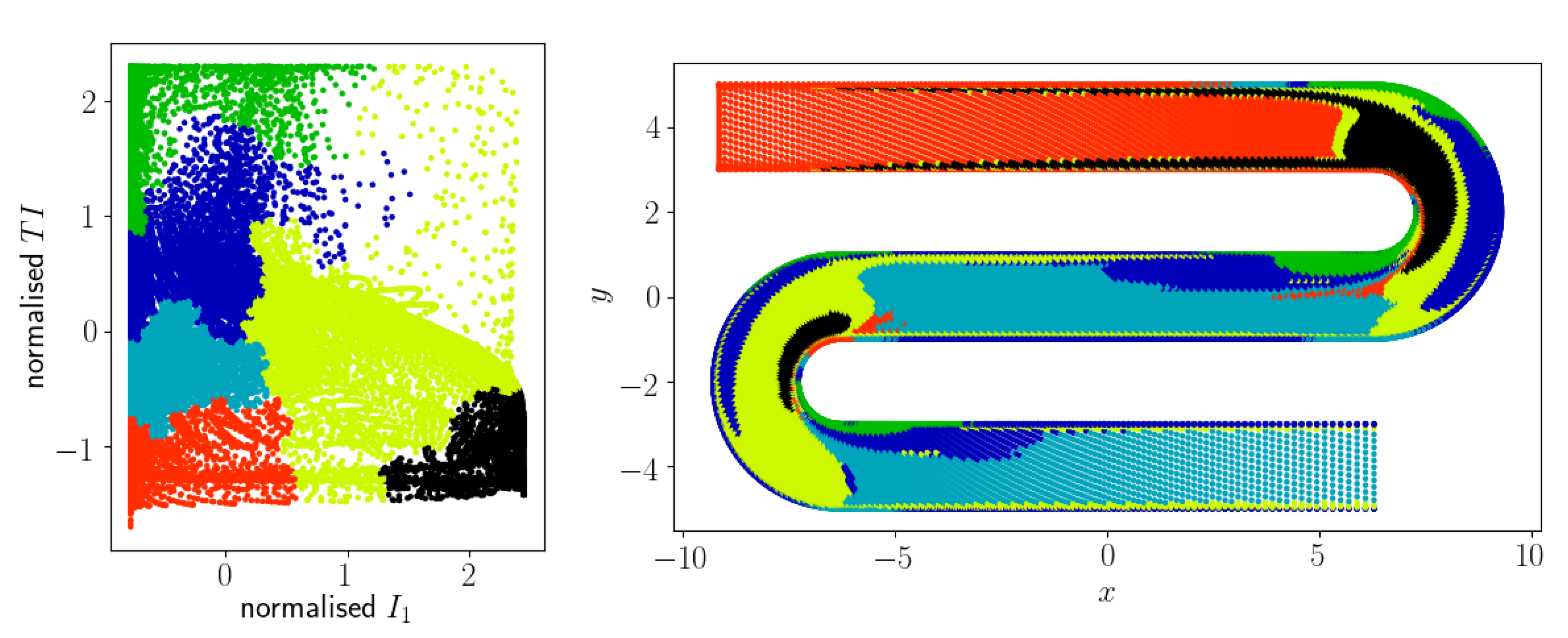
Clustering is an unsupervised learning classification technique, used in this context to identify and isolate regions of the flow characterised by the presence of specific phenomena, such as separation, curvature or high turbulence. This enables selectively training the ANN on areas that are more relevant, only using one or a combination of clusters. The features used in this process are the ones listed above and Hierarchical Agglomerative clustering algorithms are considered here, being a good compromise between complexity and ability to capture clusters of various shapes: high acceleration, curvature, high and very high mixing. The best results were found using I 1 and T I as input features and 6 clusters. The resulting classification is shown in Figure 3.
Having defined the clusters, the ANN was created using the Python library TensorFlow with the following structure: one input, two hidden layers and one output coefficient, c 1 , resulting in a formulation for the anisotropy that only includes the first term of the tensorial expansion. This very simple structure is used to define the work-flow, keeping in mind that it is very easy within TensorFlow to make the structure more complex at a later time. Despite this apparent simplicity, when building the ANN a significant number of hyperparameters need to be specified: (a) number of neurons in the hidden layers, (b) activation function for each layer, (c) number of training points, (d) optimisation algorithm, (e) hyperparameters associated to the optimisation algorithm, (f) coefficient of regularisation to ensure smoothness in the functional mapping, (g) number of iterations, (h) fraction of the feature range captured by the look-up table (to avoid that a few extreme values could deteriorate the resolution of the table in the region where most points are), (i) fraction of training points taken within the boundary layer (to avoid bias towards the wall), (j) weights assigned to the discrepancy between true values and predictions in each term of the Reynolds stress tensor, (k) input features, (l) cluster or clusters where training points are randomly selected. The choice of all these hyperparameters are made by performing a series of random searches. This is a widely used technique in Machine Learning, where a large number of models are generated by randomly picking each of these hyperparameters, either from a specified range or from a set of possible values. The loss metrics, which are a measure of how well the model is able to predict Reynolds stresses a priori, are then compared and only the most promising models are selected to be run and assessed a posteriori. Guidance is also offered by the requirement of having a smooth profile, as the RANS calculation tends to easily become unstable when strong gradients are present in the c 1 function. Further insight and understanding is then offered by the results of the RANS calculations in terms of how well these models are able to capture important aspects of the flow, such as length of the separation bubble and ability to mix the flow downstream of it. This can limit the ranges and the choice of hyperparameters and a second random search can be performed to fine tune the process. A new batch of models is reassessed a posteriori and the process can be repeated until results tend to stabilise to a performance plateau. The process not only generates a model that improves RANS predictions for the metrics of interest, but also sheds some light on the underlying physics, e.g., which clusters provide the right information for the model to perform well everywhere in the domain.

5. Results

5.1. Turbulent Channel Flow

In a straight channel the only non-negligible velocity component is the one aligned with the direction of the flow, u. In addition, as y u is the only non-zero velocity gradient, the flow is steady and ρ = 1 , most of the terms in the RANS equation and the τ i j expansion cancel out, leaving:
p x + ν 2 u y 2 τ 12 y = 0
τ 12 = 2 c 1 k s 12
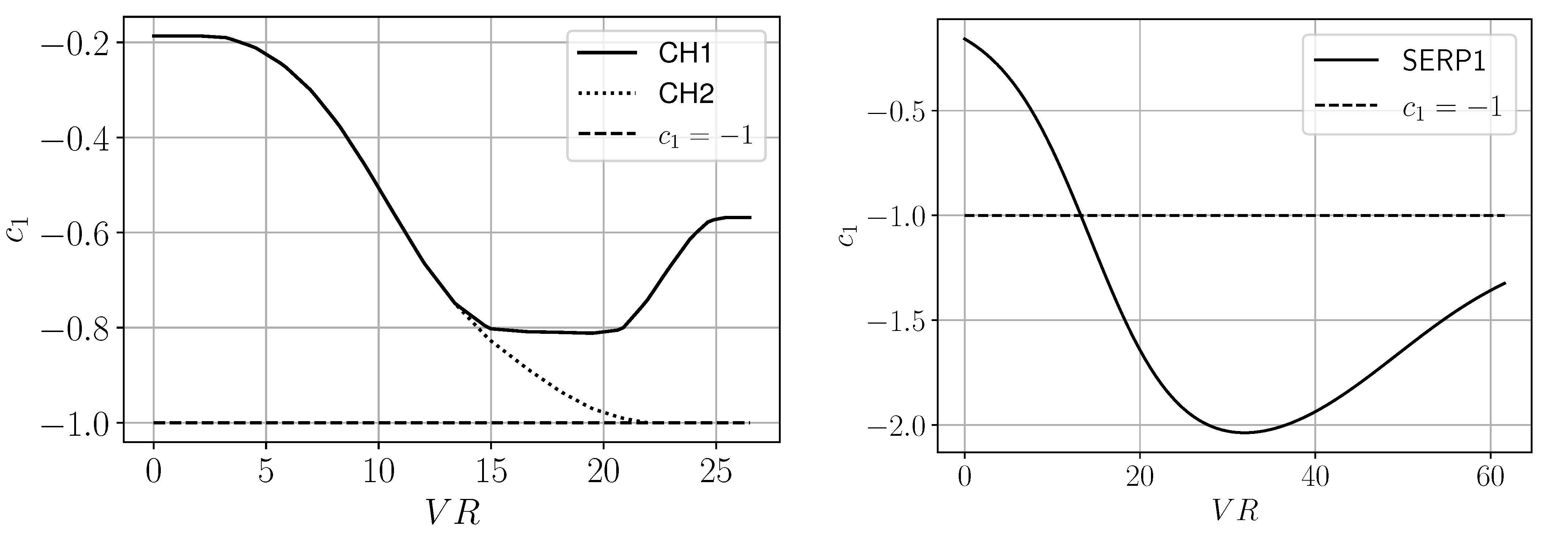
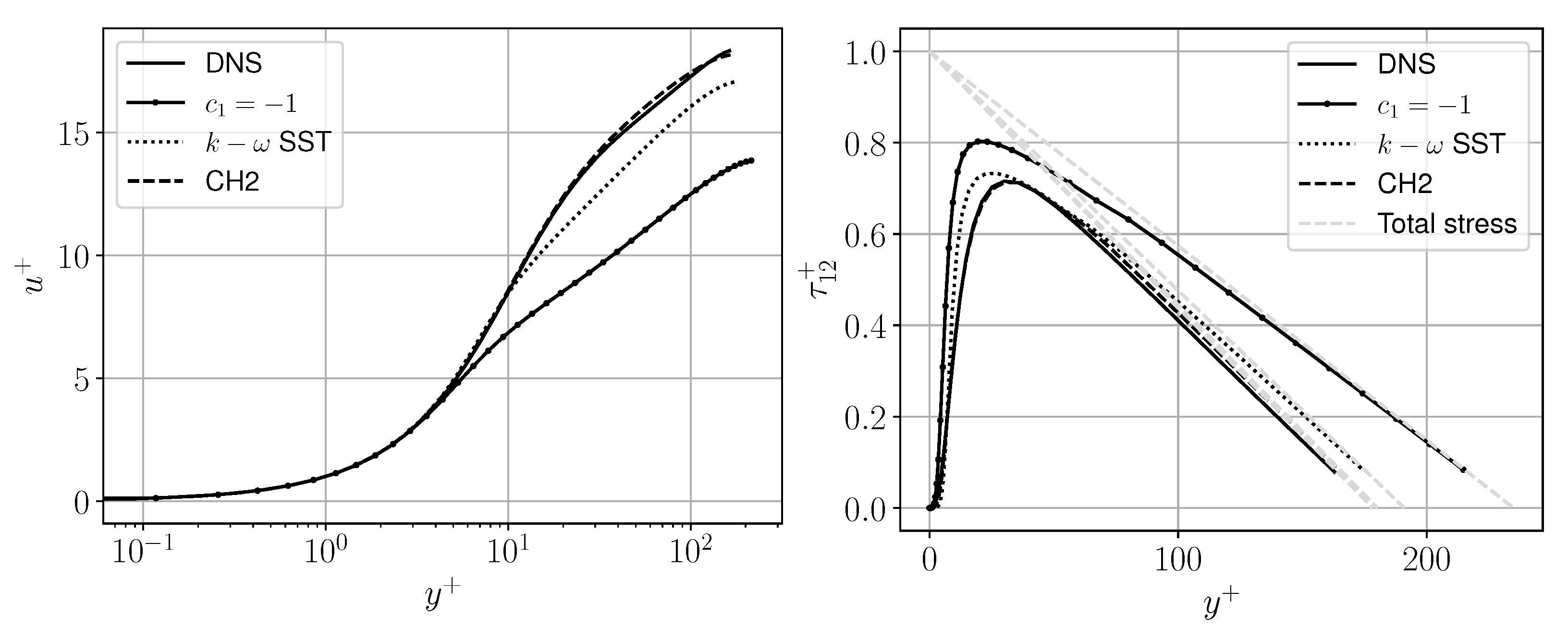
As τ 12 , k and s 12 are available from the DNS data, it is possible to infer the distribution of c 1 that would make (4) hold to any degree of accuracy. In this simple case, applying the ML process we described is equivalent to look for a non-linear best fit to a specified smoothness (tuned through the regularisation hyper-parameter) of the point-wise mapping c 1 i ( f 1 i ) for all points in the training set, with f 1 being the flow feature chosen to train the ANN. Due to the very limited amount of data available, clustering was not applied to this test case. The flow feature that showed the best ability to predict τ 12 and quite straightforwardly u from (4) is the viscosity ratio V R . In particular two models have been selected, the one coming directly out of the ANN (referred to as CH1), and one where c 1 is blended to 1 for high values of V R , in order to recover the Boussinesq approximation (CH2). Figure 4 (left) shows the graphical representation of the two models, while Figure 5 shows the comparison between DNS, ML models and baseline RANS in terms of u + (left) and τ 12 + (right). The RANS calculations were run imposing a pressure gradient along the duct, adjusting the molecular viscosity for c 1 = 1 and k ω SST in order to keep the same Reynolds number, as the bulk mean velocity differed more than 2% from the DNS. The difference between CH1 and CH2 in the velocity and τ 12 profiles is small and only CH2 is shown in Figure 5. To have a quantitative metric for the improvement achieved, the following parameter is defined:
Δ = D | ϕ m o d e l ϕ D N S | d D D | ϕ D N S | d D
where D is the domain and ϕ a flow variable of interest. Table 1 summarises how this metric compares for the different models for u and τ 12 .

5.2. Serpentine Passage

For the serpentine passage the abundance of potential training points compared to the channel made it possible to (a) take advantage of clustering to further explore training options and (b) train (within the selected clusters) on the first half of the geometry only to see if the constitutive relationship is able to improve the flow predictions also in a region of the domain not used for training. From the a posteriori results of the random search it was observed that:
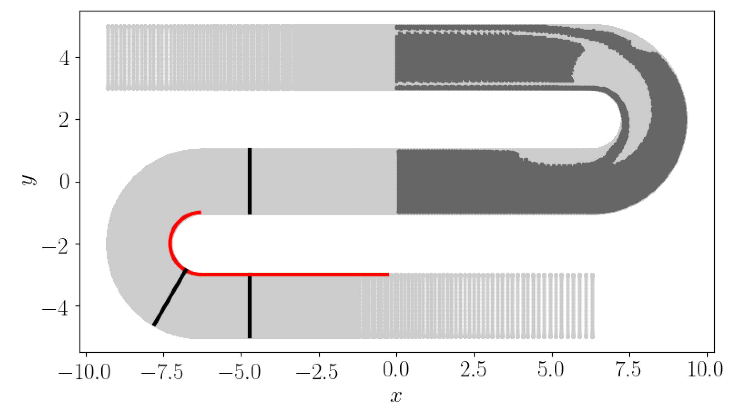
  • The best results are achieved excluding the high strain and separation clusters (black and dark green respectively in Figure 3) from the training set. This finding is further detailed in the Discussion section. The corresponding training set is shown in Figure 6.
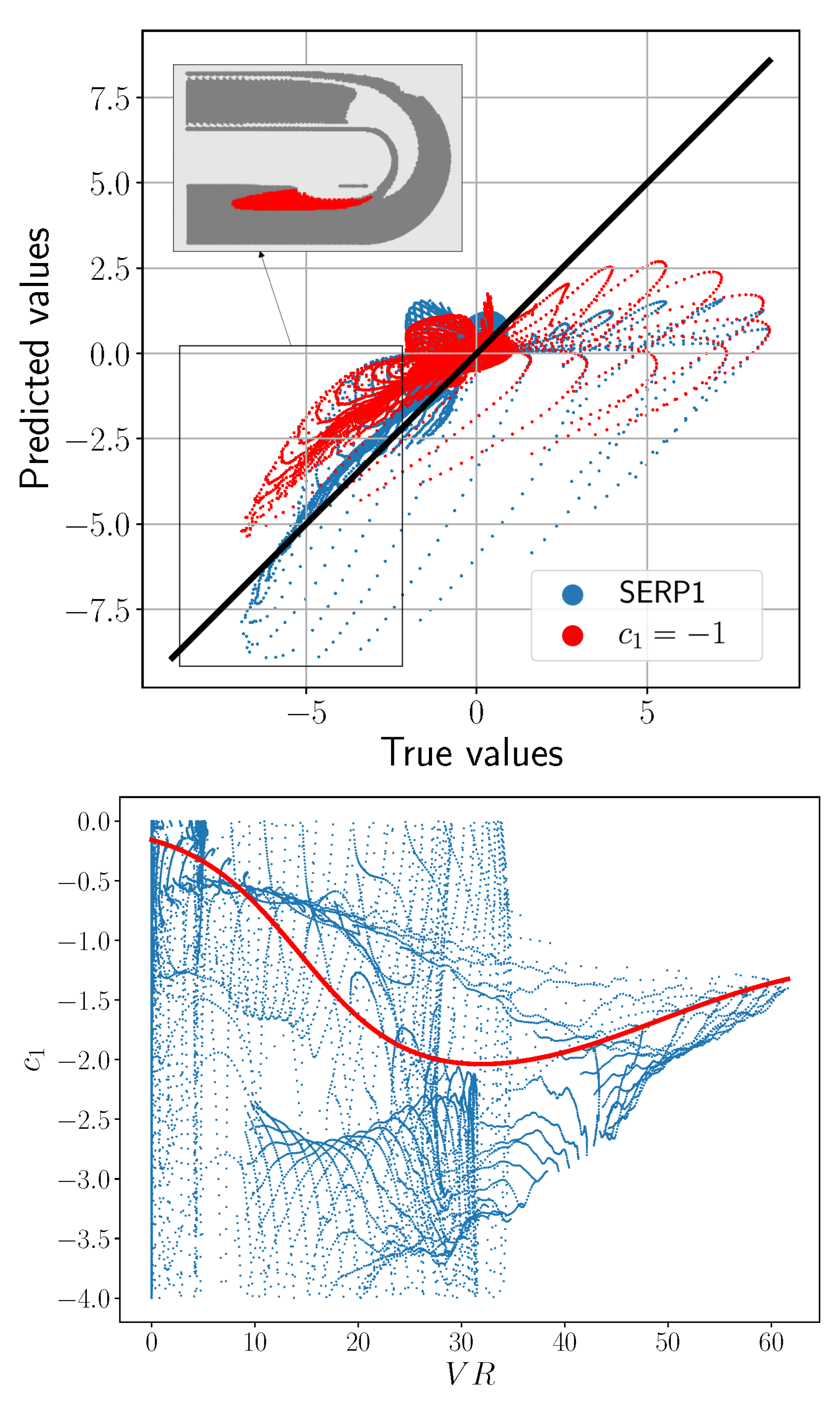
  • The input flow feature that performed best is again V R , as seen for the channel. Up to V R 15 the qualitative behaviour of the best serpentine model, referred to as SERP1, is similar to CH1; however, after that, the coefficient becomes even stronger ( c 1 = 2 ) before settling at around 1.3 (Figure 4, right).
  • Regularisation is essential to guarantee sufficient smoothing; less regularised models that seem to have a good performance a priori failed to meet expectations when assessed a posteriori.
  • The best results were found with two hidden layers, with 4 and 5 neurons, respectively. This illustrates that significant improvements can be achieved even with relatively simple ANN structures.
Figure 7 (bottom) illustrates for each point of the training region how the chosen feature, V R , correlates with the ideal value of c 1 , the one that would make the predicted τ 12 , the most impactful Reynolds stress term, match the DNS value. Overlapped in red is the SERP1 model. It can be seen how the scatter is significant, especially in the mid-range, where we can also expect more model uncertainty. Figure 7 (top) shows how in the a priori analysis the true to predicted values of τ 12 redistribute when going from a uniform coefficient c 1 = 1 to the SERP1 predictions. The difference can be quantified in terms of the R 2 score going from 0.44 to 0.51, with a noticeable effect at the separation bubble interface (highlighted in the figure). Albeit this can be seen as a relatively modest improvement, it is sufficient to strongly influence the a posteriori performance, which is ultimately the goal of the study. This can be seen in Figure 8, where SERP1 is compared to DNS, baseline RANS and CH2 in terms of velocity magnitude traverses at different locations and wall shear stress on the separation region after the second bend. The predicted separation bubble length, as well as velocity and τ 12 at these locations is summarised in Table 2.

6. Discussion

The best ML model for both test cases presents a c 1 that is reduced to ≈ 0.15 when V R approaches zero. This is equivalent to saying that the Reynolds stress predictions are not proportional to ν t , but tend to zero faster, particularly near the wall. For the channel this has a similar role to the one played by the limiter on ν t in the k ω SST. The results described in the previous section show that flow field predictions can significantly be improved by a relatively small modification in the way turbulence is modelled. This can be noticed particularly for the serpentine test case on the separation bubble, in terms of shape and length, although the ANN training did not see any point within that region. More surprisingly, a posteriori model performance degraded when including separation in the training set. The following line of reasoning provides an interpretation for this phenomenon: the ability to predict the shape of the separation bubble mainly relies on having a good estimate of the turbulent mixing in the flow reaching the separation point and, more importantly, just outside the rear part of the bubble, as this strongly influences the reattachment point. However, adding points within the separation region in the training does not provide any benefit and has instead the effect of forcing a less than optimum c 1 in the most influencing areas of the domain. The possibility of training different models for attached and separated regions and applying them zonally has not been investigated in this study. In using k ω as the underlying turbulence model, an important assumption is that the k field obtained by solving the steady k equation:
u j k x j = P k β * k ω + x j ν + σ k ν t k x j
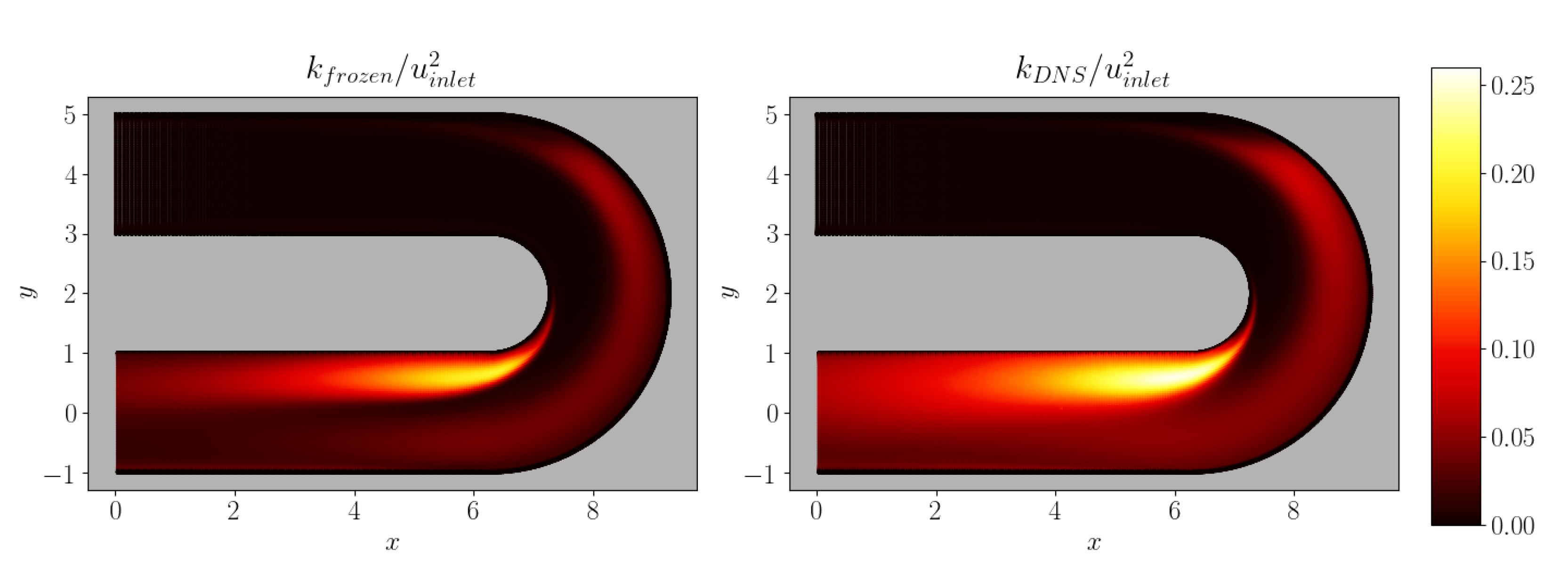
with u i , x j u i and τ i j from the DNS calculation (referred to as the frozen field), converges to a distribution that is close to the DNS one (for which k = 1 2 ( u u ¯ + v v ¯ + w w ¯ ) is known). While for the channel this assumption is verified, for the serpentine there are some significant quantitative and qualitative differences (Figure 9):
The levels of k are lower for the frozen field by a factor of approximately 1.7 on average and the diffusion does not seem to allow enough mixing after the bend. The root cause for this can be identified in a wrong prediction of the k budget P k β * k ω and a poor level of k turbulent mixing. However, it would not be consistent to use the DNS distribution of k, ω and turbulent transport in the training phase, as this is not what is available to the RANS solver, which computes k and ω from the transport equations. The ANN converges to a stronger c 1 , in order to compensate for the lower values of k and still achieves a good approximation of the target τ i j . When compared to k ω SST, this has the effect of enhancing the mixing outside of the separation bubble, along the second straight and on the second bend, all regions where baseline RANS predictions were particularly weak. An attempt was made to apply the SERP1 model back to the turbulent channel. Having a similar trend at the low end of the V R range, the near wall behaviour is still captured well. However, as the k predictions from the frozen field for this case were already close to the DNS, the overcompensation at high V R results in the detrimental effect of flattening the u profile towards the centreline.

7. Conclusions

In this paper, we demonstrated how we can use high fidelity DNS data and a TensorFlow Machine Learning framework to generate alternative Reynolds stress anisotropy formulations that replace the standard Boussinesq approximation. It is observed that this is not a blind process, as the many hyperparameters required to set up the ANN have a strong influence on the outcome, and not carefully considering the regularisation, the relative importance of training areas and the choice of input flow features can have a strong detrimental effect on a posteriori performance. Clustering has been identified as a particularly useful tool to selectively train the ANN on limited portions of the domain. It is also emphasised how a priori assessment can provide only a partial view, as the propagation of the error from τ i j to velocity components is non-linear and often erratic. In selecting the final model it is, therefore, critical to perform subsequent random searches, testing the most promising ones by running a RANS and looking at flow fields predictions. This method achieved significant progresses for the two test cases examined in this paper:
  • The channel flow velocity profile predictions reached a discrepancy (based on Equation (5)) to the DNS of 0.026 for CH1 and 0.019 for CH2 from a value of 0.041 for the k ω SST and 0.213 for the k ω SST without the limiter on ν t .
  • For the serpentine the difference to the DNS in the length of the second separation bubble went from 2.95 for the k ω SST to 0.47 for SERP1. The velocity discrepancy (based on Equation (5)) for three representative traverses (Figure 6) was also reduced by 65.2%, 74.1% and 88.4%, respectively.
These results show the vast potential of this method, which is targeted to specific applications. In contrast, the poor performance of SERP1 on the turbulent channel case highlights how the user should be conscious of the limitations of a model from a physics perspective, such as overcompensation. Future work will aim at including more than one input feature and other terms in the tensorial expansion, as well as expanding the work-flow to additional flow phenomena, e.g., mixing and 3D corner vortices.

Author Contributions

Conceptualization, Y.F.M., F.M., R.V., P.A.; methodology, Y.F.M., F.M., P.A.; software, Y.F.M., A.C., P.A.; validation, Y.F.M.; formal analysis, Y.F.M.; investigation, Y.F.M., E.A.d.T.O.; resources, R.V., F.M., P.A.; data curation, Y.F.M.; writing—original draft preparation, Y.F.M.; writing—review and editing, Y.F.M.; visualization, Y.F.M., E.A.d.T.O.; supervision, R.V., F.M., P.A.; project administration, R.V., F.M., P.A.; funding acquisition, R.V. All authors have read and agreed to the published version of the manuscript.

Funding

This research received funding from the Aerospace Technology Institute (ATI)/Innovate UK programme “FANFARE”.

Institutional Review Board Statement

Not applicable.

Informed Consent Statement

Not applicable.

Conflicts of Interest

The authors declare no conflict of interest.

Abbreviations

The following abbreviations are used in this manuscript:
DNSDirect Numerical Simulation
RANSReynolds-Averaged Navier–Stokes
CFDComputational Fluid Dynamics
MLMachine Learning
GEPGene Expression Programming
ANNArtificial Neural Network
Nomenclature
kturbulent kinetic energy
ω turbulent specific dissipation
ρ density
ϵ turbulent dissipation
τ i j Reynolds stress tensor: u i u j ¯
τ i j i s isotropic Reynolds stress
a i j anisotropy tensor
ν t turbulent viscosity
S i j strain rate tensor
c q tensor expansion coefficients
V i j q tensor basis
s i j non dimensional strain rate tensor
w i j non dimensional rotation rate tensor
x j u i velocity gradient tensor
u , v , w velocity fluctuations
ν laminar viscosity
d w distance from the wall
u i velocity components
I 1 , I 2 velocity gradient invariants
V R viscosity ratio
R T local turbulent Reynolds number
T I turbulence intensity
P k k production
β * , σ k k ω SST model constants

References

  1. Launder, B.; Spalding, D.B. The Numerical Computation of Turbulent Flows. Comput. Methods Appl. Mech. Eng. 1974, 3, 269–289. [Google Scholar] [CrossRef]
  2. Wilcox, D. Turbulence Modeling for CFD; Number v. 1 in Turbulence Modeling for CFD; DCW Industries: La Canada, CA, USA, 2006. [Google Scholar]
  3. Weatheritt, J.; Sandberg, R. A novel evolutionary algorithm applied to algebraic modifications of the RANS stress-strain relationship. J. Comput. Phys. 2016, 325, 22–37. [Google Scholar] [CrossRef]
  4. Pope, S.B. A more general effective-viscosity hypothesis. J. Fluid Mech. 1975, 72, 331–340. [Google Scholar] [CrossRef] [Green Version]
  5. Weatheritt, J.; Pichler, R.; Sandberg, R.; Laskowski, G.; Michelassi, V. Machine learning for turbulence model development using a high-fidelity HPT cascade simulation. In Proceedings of the ASME Turbo Expo, Charlotte, NC, USA, 26–30 June 2017. [Google Scholar]
  6. Moxey, D.; Cantwell, C.; Bao, Y.; Cassinelli, A.; Castiglioni, G.; Chun, S.; Juda, E.; Kazemi, E.; Lackhove, K.; Marcon, J.; et al. Nektar++: Enhancing the capability and application of high-fidelity spectral/hp element methods. Comput. Phys. Commun. 2020, 249, 107110. [Google Scholar] [CrossRef]
  7. Mansour, N.N.; Kim, J.; Moin, P. Reynolds-stress and dissipation-rate budgets in a turbulent channel flow. J. Fluid Mech. 1988, 194, 15–44. [Google Scholar] [CrossRef] [Green Version]
  8. Cassinelli, A.; Montomoli, F.; Adami, P.; Sherwin, S.J. High Fidelity Spectral Hp Element Methods For Turbomachinery. In Proceedings of the ASME Turbo Expo, Oslo, Norway, 11–15 June 2018. [Google Scholar]
  9. Laskowski, G.; Durbin, P.A. Direct numerical simulations of turbulent flow through a stationary and rotating infinite serpentine passage. Phys. Fluids 2007, 19, 015101. [Google Scholar] [CrossRef] [Green Version]
  10. Cassinelli, A.; Xu, H.; Montomoli, F.; Adami, P.; Vazquez Diaz, R.; Sherwin, S.J. On the Effect of Inflow Disturbances on the Flow Past a Linear LPT Vane Using Spectral/hp Element Methods. In Proceedings of the ASME Turbo Expo 2019, Phoenix, AZ, USA, 17–21 June 2019. [Google Scholar]
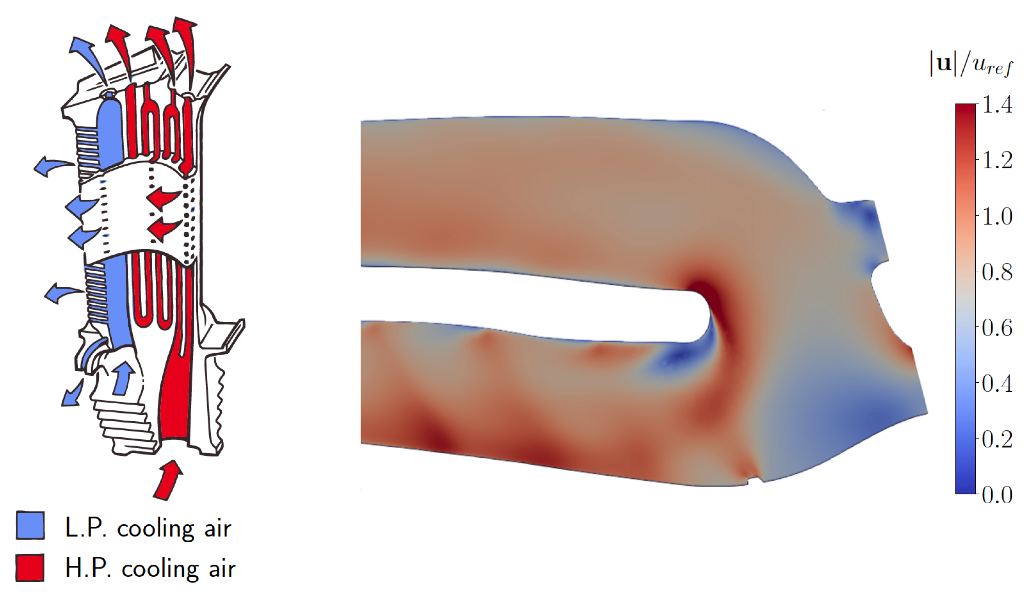
Figure 1. High pressure turbine cooling system (left) and CFD of internal passage (right).
Ijtpp 06 00017 g001
Figure 2. Q-Criterion iso-contours ( Q = 100 ) and time average velocity along second bend.
Ijtpp 06 00017 g002
Figure 3. Cluster classification in feature space (left) and physical space (right).
Ijtpp 06 00017 g003
Figure 4. c 1 models: CH1, CH2 for the channel (left) and SERP1 for the serpentine (right).
Ijtpp 06 00017 g004
Figure 5. Channel model comparison in terms of u (left) and τ 12 (right).
Ijtpp 06 00017 g005
Figure 6. Training regions highlighted in dark grey and location of velocity (black lines) and wall shear stress (red line) comparisons.
Ijtpp 06 00017 g006
Figure 7. SERP1 a priori assessment: true to predicted τ 12 with comparison to Boussinesq approximation (top) and SERP1 best fit of ideal c 1 (bottom).
Ijtpp 06 00017 g007
Figure 8. Velocity magnitude comparison at 3 different locations from upstream: top left, bottom left, top right (cfr. Figure 6) and wall shear stress along the second bend: bottom right.
Ijtpp 06 00017 g008
Figure 9. Comparison between DNS and frozen k field.
Ijtpp 06 00017 g009
Table 1. Discrepancy Δ between DNS and different models for the channel test case.
DNS c 1 = 1 k ω SSTCH1CH2
u-0.2130.0410.0260.019
τ 12 -0.2140.1060.0250.038
Table 2. Length of the separation bubble in non-dimensional units and discrepancy Δ between DNS and different models for the serpentine test case.
DNS c 1 = 1 k ω SSTSERP1CH2
Sep. bubble length2.373.165.322.844.67
| u | 1st traverse Δ -0.08040.10750.03750.1014
| u | 2nd traverse Δ -0.08560.12620.03270.1066
| u | 3rd traverse Δ -0.09040.24450.02840.1893
Publisher’s Note: MDPI stays neutral with regard to jurisdictional claims in published maps and institutional affiliations.