
Centrifugal Compressor Polytropic Performance—Improved Rapid Calculation Results—Cubic Polynomial Methods


Abstract
1. Introduction
1.1. Polytropic History
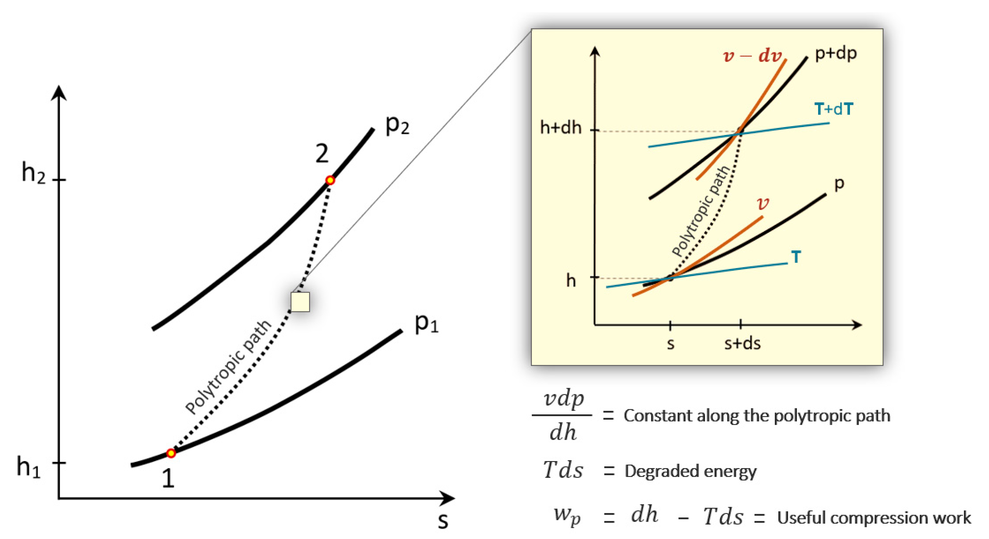
1.2. Polytropic Process
2. Polytropic Path: Polynomial Approximation Methods
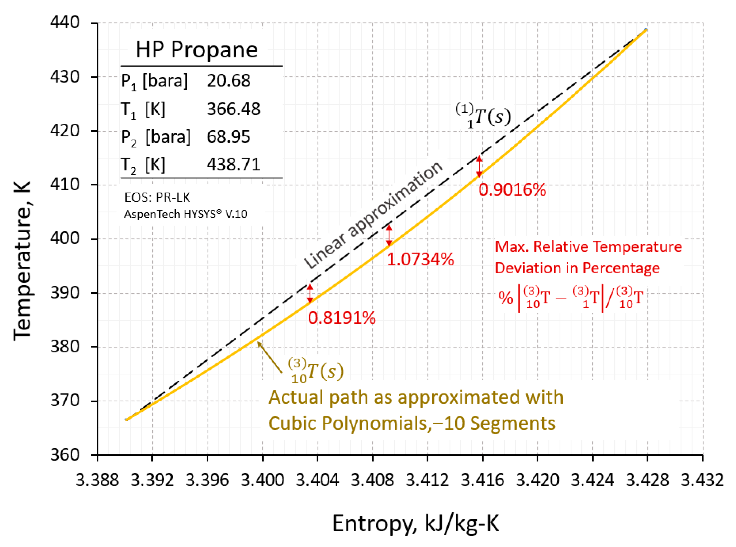
2.1. Temperature-Entropy Polytropic Path Approximation: Linear Polynomial Endpoint Method
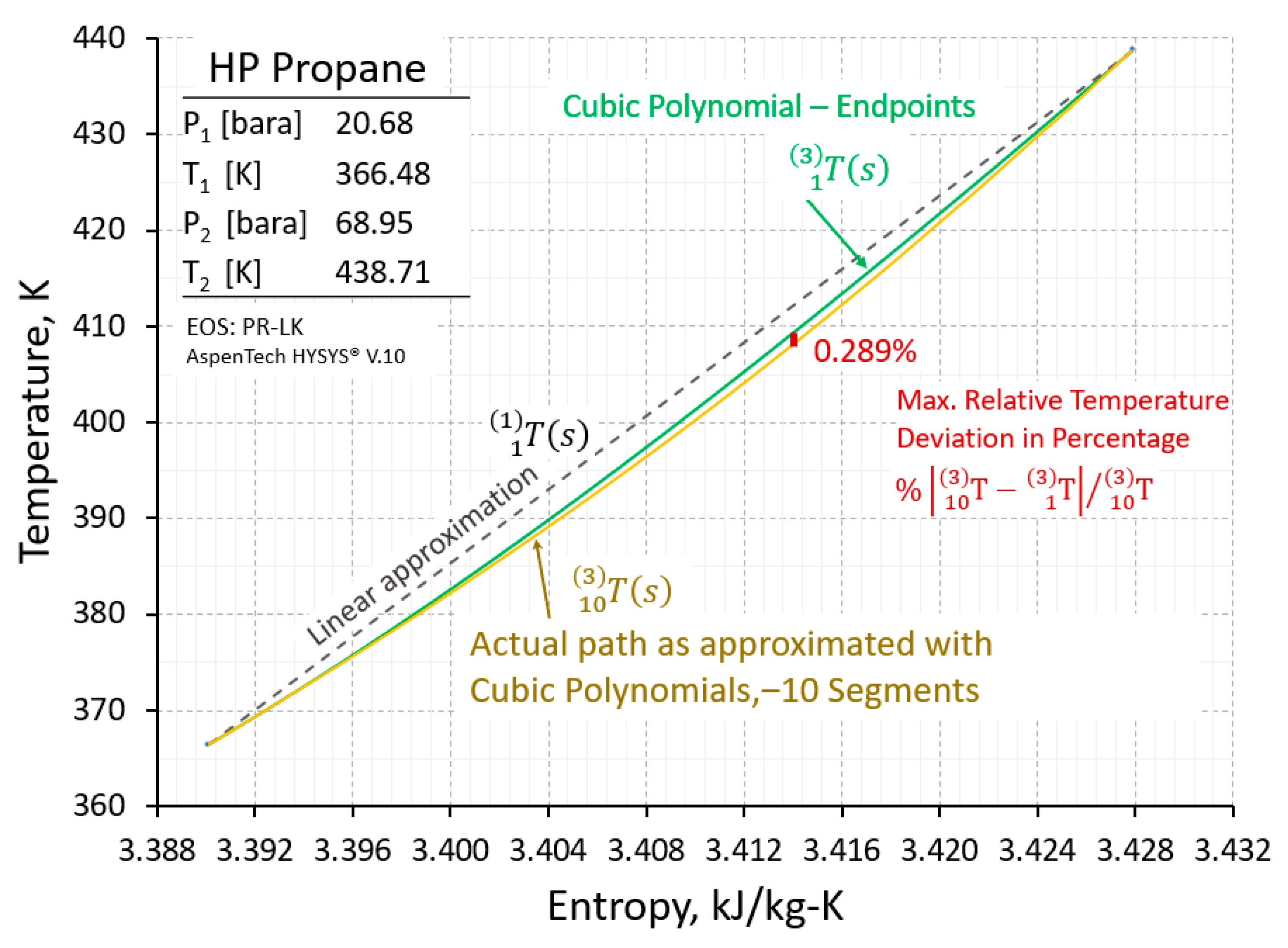
2.2. Temperature-Entropy Polytropic Path Approximation: Cubic Polynomial Endpoint Method
3. Polytropic Efficiency Calculation
3.1. Polytropic Efficiency Calculation: Linear Polynomial Endpoint Method
3.2. Polytropic Efficiency Calculation: Taher–Evans Cubic Polynomial Endpoint Method
3.3. Polytropic Efficiency Calculation: Linear Multistep Method
3.4. Polytropic Efficiency Calculation: Taher–Evans Cubic Polynomial Multi-Segment Method
3.4.1. Polytropic Efficiency Calculation Procedure: Taher–Evans Cubic Polynomial Multi-Segment Method
- (1)
- Determine an initial estimate of polytropic efficiency by assuming in the relationship (45) for the cubic polynomial endpoint method.Note: for the purpose of compressor performance testing, the initial value of the efficiency is the expected efficiency provided by the compressor manufacturer.
- (2)
- Select the number of segments ().There are different ways to select intermediate knots. In this paper, the overall pressure ratio is divided across the number of segments () to determine equal pressure ratio steps as shown in the next step.
- (3)
- Use “” number of equal pressure ratio segments..
- (4)
- Use Equation (29) to estimate the initial value of segment outlet temperature. (This requires a solution to the cubic polynomial endpoint method).Note: steps 1 through 4 are only required for the initialization of the solution algorithm.
- (5)
- Calculate segment temperature rise,
- (6)
- Calculate the segment polytropic efficiency using the relationship (45).
- (7)
- Calculate efficiency deviation from the initially estimated polytropic efficiency from step 1.
- (8)
- Iterate segment outlet temperature to match assumed efficiency.Note: different root finding algorithms may be used to optimize iterations for segment outlet temperature.Note: the acceptable efficiency convergence should be set less than
- (9)
- Move to next segment using outlet conditions of previous segment as inlet conditions.
- (10)
- Repeat steps 5 through 9 for each segment.
- (11)
- Compare final discharge temperature with the given value,
- (12)
- If step 11 result is not within a small tolerance, iterate efficiency and determine new values for coefficients A, B, C and D.
- (13)
- Repeat steps 5 through 11 until agreement is reached within the tolerance.Note: the acceptable convergence from the given discharge temperature should be set less than
3.4.2. Distinction between Cubic Interpolation and Approximation
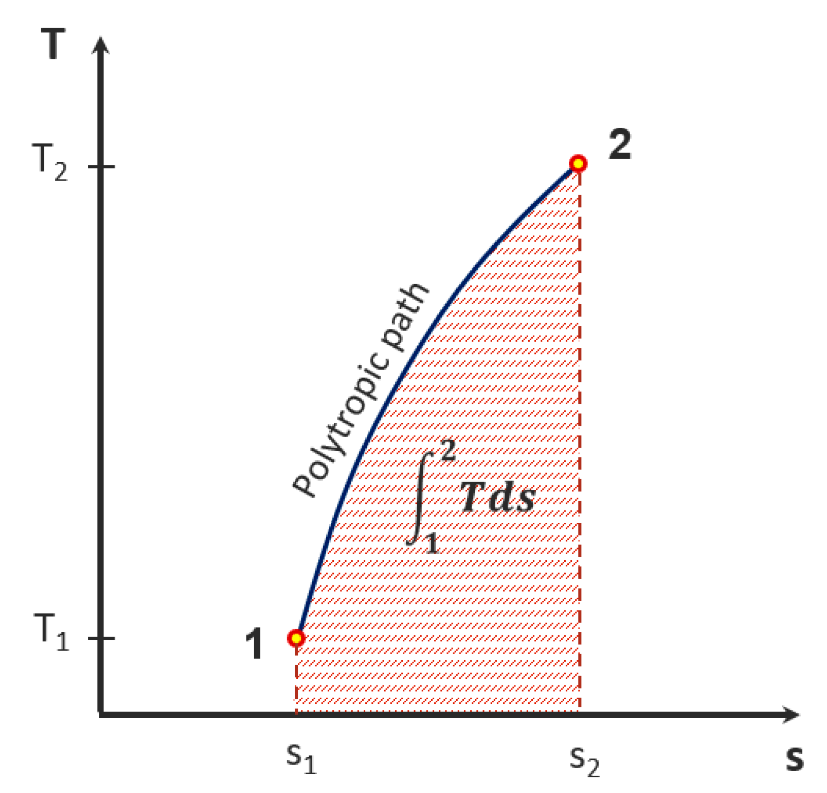
4. Polytropic Path on Temperature-Entropy Diagram
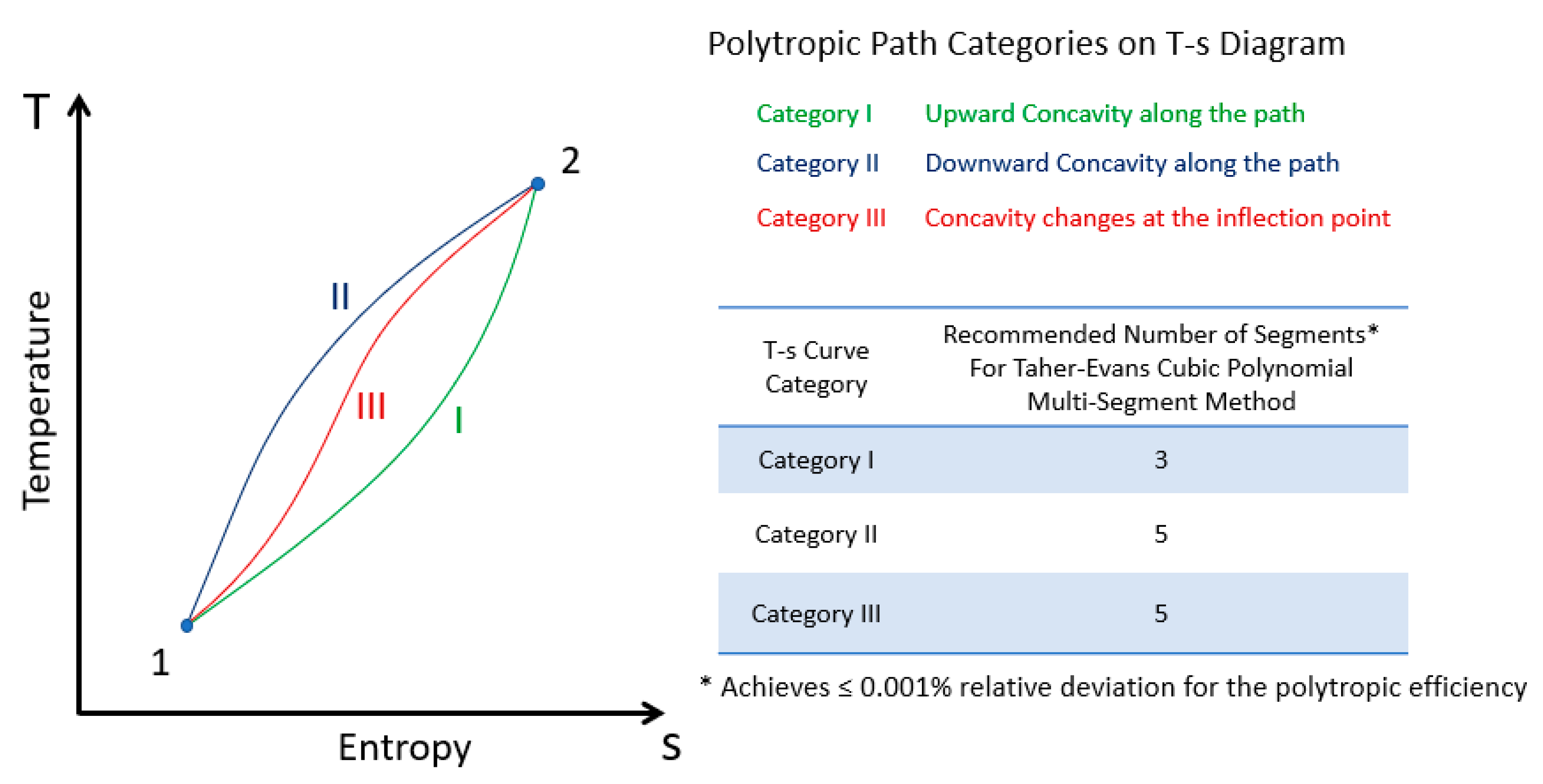
- If is out of the range of and the upward concavity of the cubic polynomial approximant, is unchanged along the path. See Figure 10 curve I.
- If is out of the range of and the downward concavity of the cubic polytropic approximant, is unchanged along the path. See Figure 10 curve II.
- If the concavity of the cubic polytropic approximant, changes at the inflection point . See Figure 10 curve III.
5. Enthalpy Change with Entropy along the Polytropic Path
6. Comparison of Cubic and Linear Polynomial Results
7. Conclusions
- The Taher–Evans Cubic Polynomial method (TE-CP), defined, described and tested herein, illustrates that a highly accurate calculation method for real gas centrifugal compressor polytropic performance efficiency has been developed and implemented that employs a temperature—entropy cubic polynomial path function.
- ○
- Both endpoint and sequential segment versions are described and tested.
- ○
- Previously published polytropic efficiency calculation methods including first degree linear polynomial methods are shown to be less accurate and/or slower to achieve a solution than Taher–Evans Cubic Polynomial methods.
- ○
- The TE-CP methods’ superior results are due to the cubic polynomial path having additional thermodynamic constraints applied to more accurately approximate the actual path slope at any point along the path. Determination of path slope at the compression endpoints is independent of performance calculation method.
- ○
- T-s polytropic path curve shapes can be determined from derivatives of the cubic polynomial path equation and are indicative of calculation relative difficulty. The curve shape is used as a criterion to select the required number of cubic segments. No other polytropic method can provide such a mathematical and thermodynamic insight into the fluid compression process.
- ○
- The number of T-s path cubic polynomial segments required to achieve an acceptable relative deviation ≤0.001% for polytropic efficiency is three segments for category I and five segments for categories II and III curve shapes.
- ○
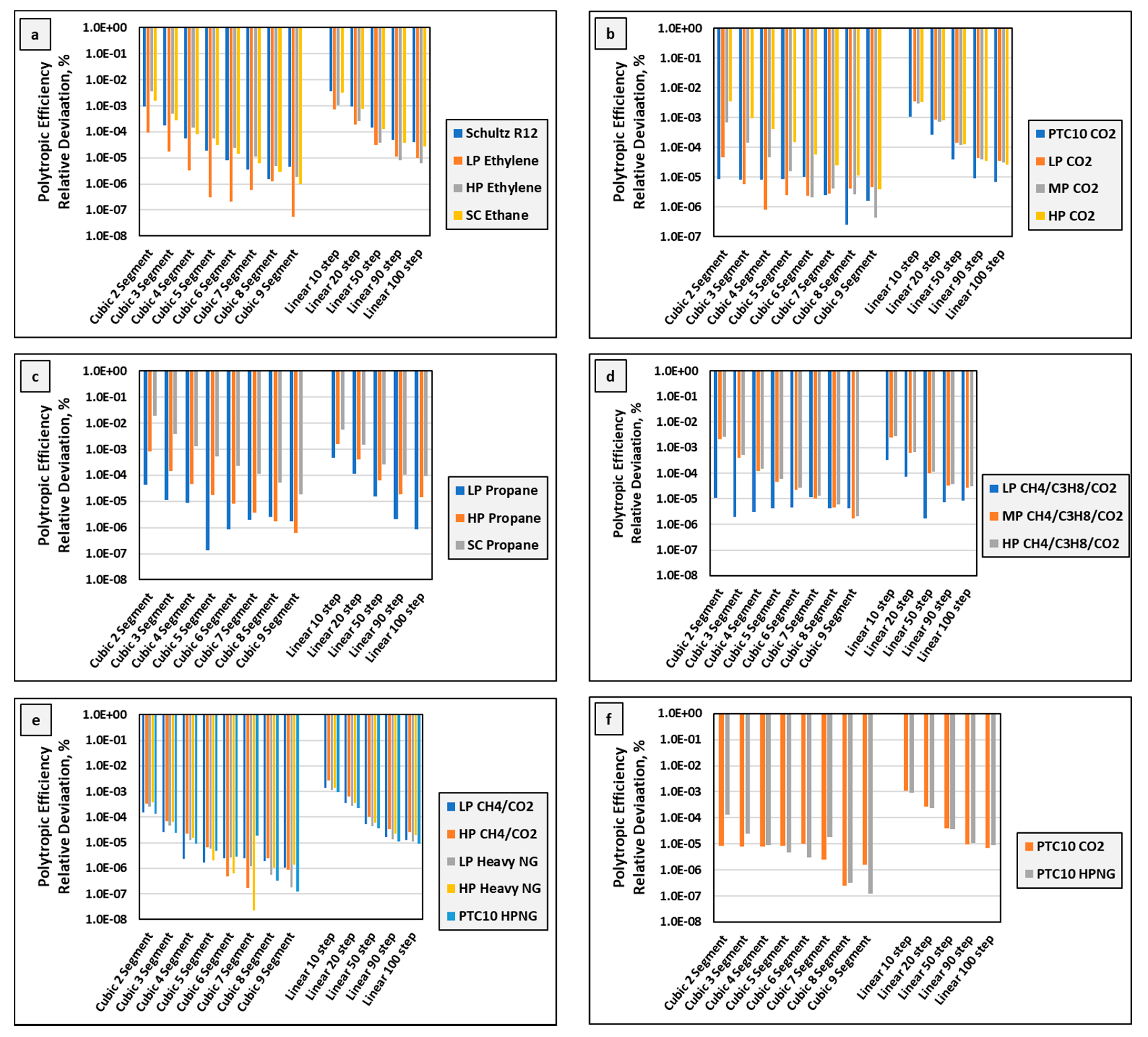
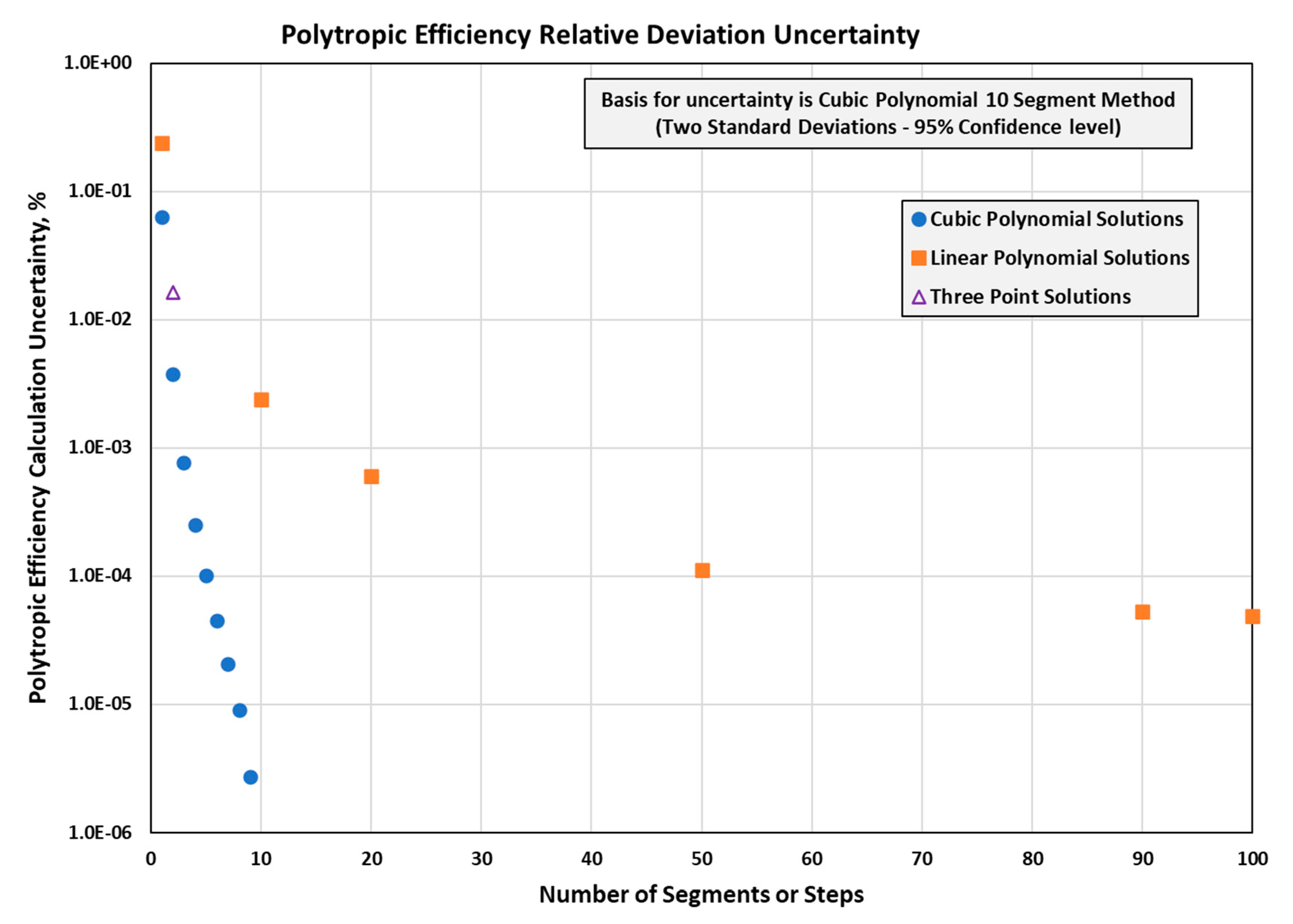
- As shown in Figure A10, the cubic polynomial methods provide low uncertainty with only a few cubic segments. Uncertainty is based upon polytropic efficiency relative deviation, and its magnitude is related to the size of the statistical population.
- ○
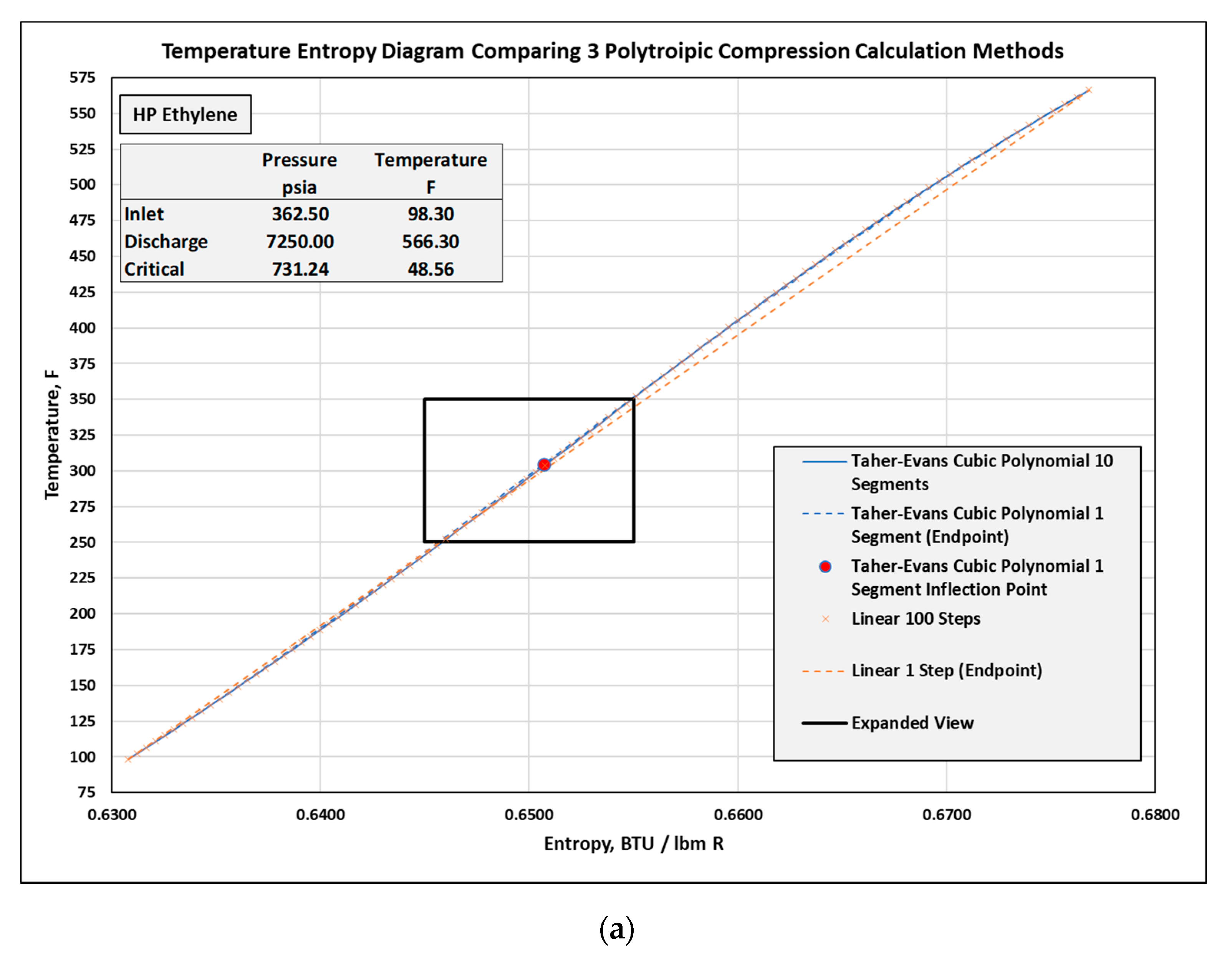
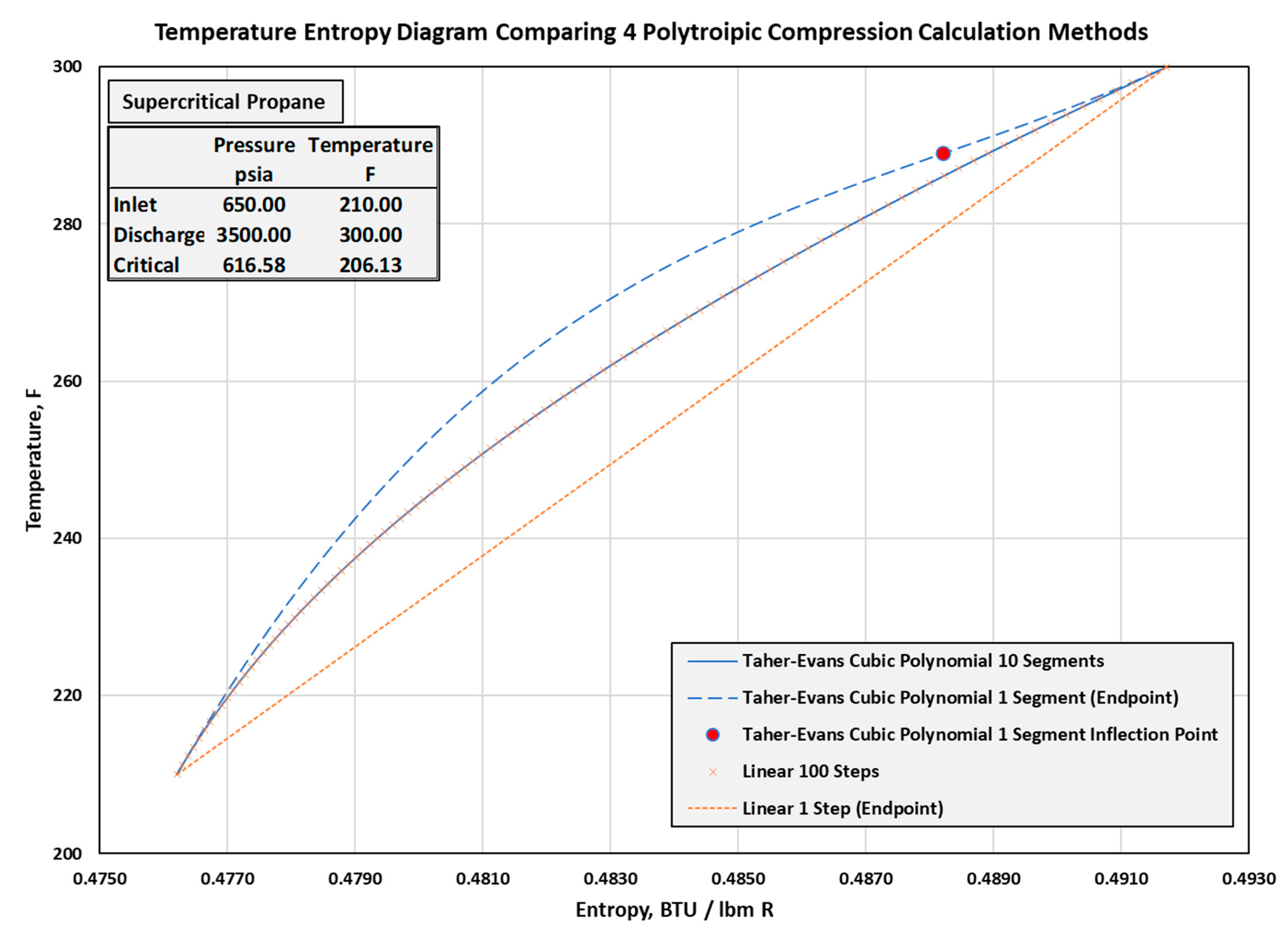
- Cubic polynomial methods provide continuous equations to plot the polytropic path on T-s and h-s diagrams. This is a very unique feature of the cubic polynomial method that enables visualizing the polytropic path.
- ○
- The cubic path coefficients (A, B, C, and D) in Equation (12) provide meaningful insights about the behavior of the polytropic path on the temperature-entropy diagram.
- ○
- The Taher–Evans Cubic Polynomial methods are highly suitable for application to compressor performance testing according to ASME PTC 10 [4].
- Cubic and linear polynomial calculation methods have been extensively documented and compared.
- ○
- Polytropic efficiency calculations have been reviewed for 17 methods across 115 example cases yielding a total of 1955 independent calculations that validate superior results are achieved when using both endpoint and sequential segment Taher–Evans Cubic Polynomial (TE-CP) polytropic path methods. A total of 22 fluids were employed including seven pure fluids and 15 fluid mixtures to cover wide ranges of mole weight and critical pressures and temperatures.
- ○
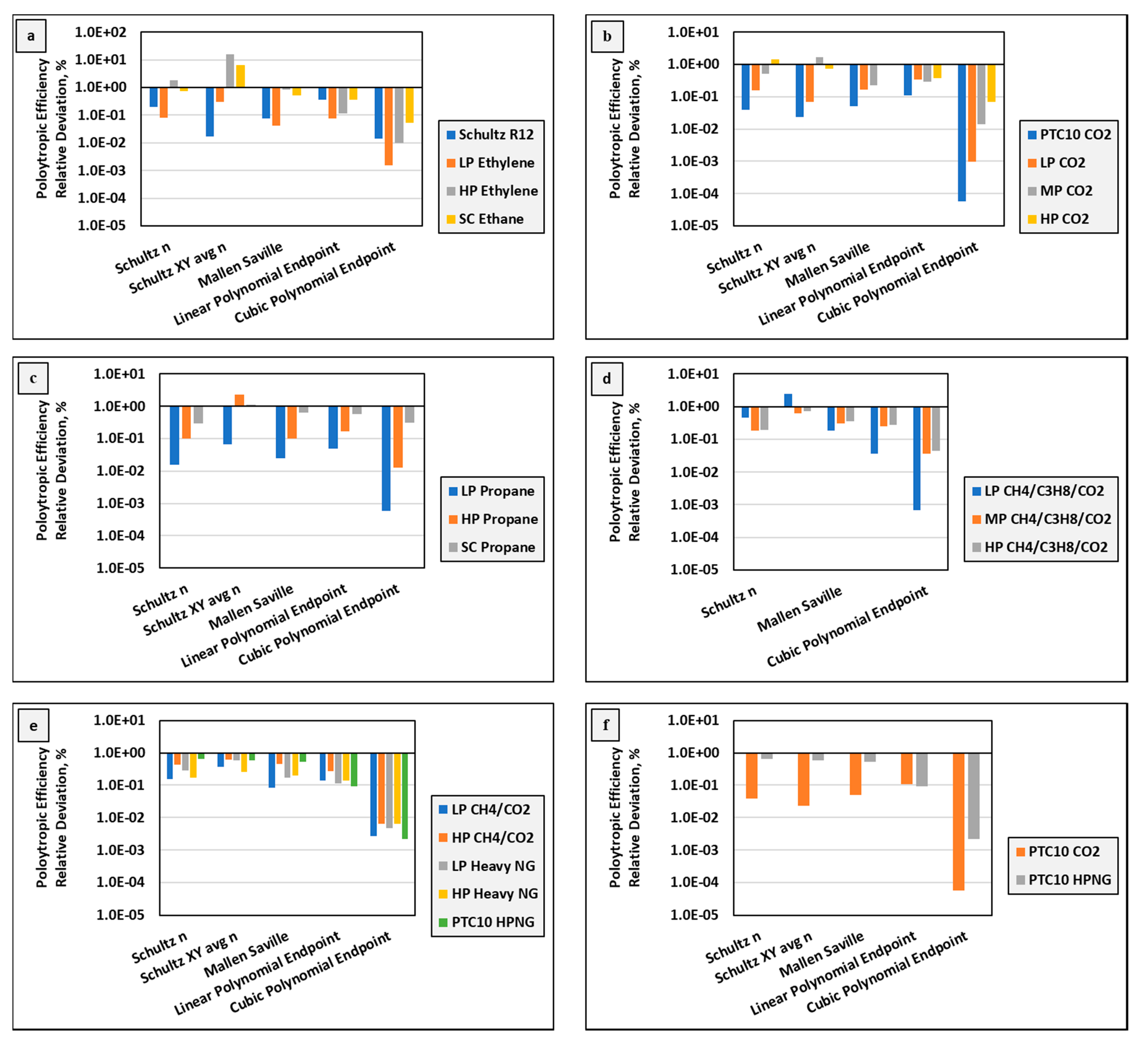
- Cubic polynomial endpoint path methods were demonstrated to achieve better accuracy than any other endpoint polytropic efficiency calculation method.
- ○
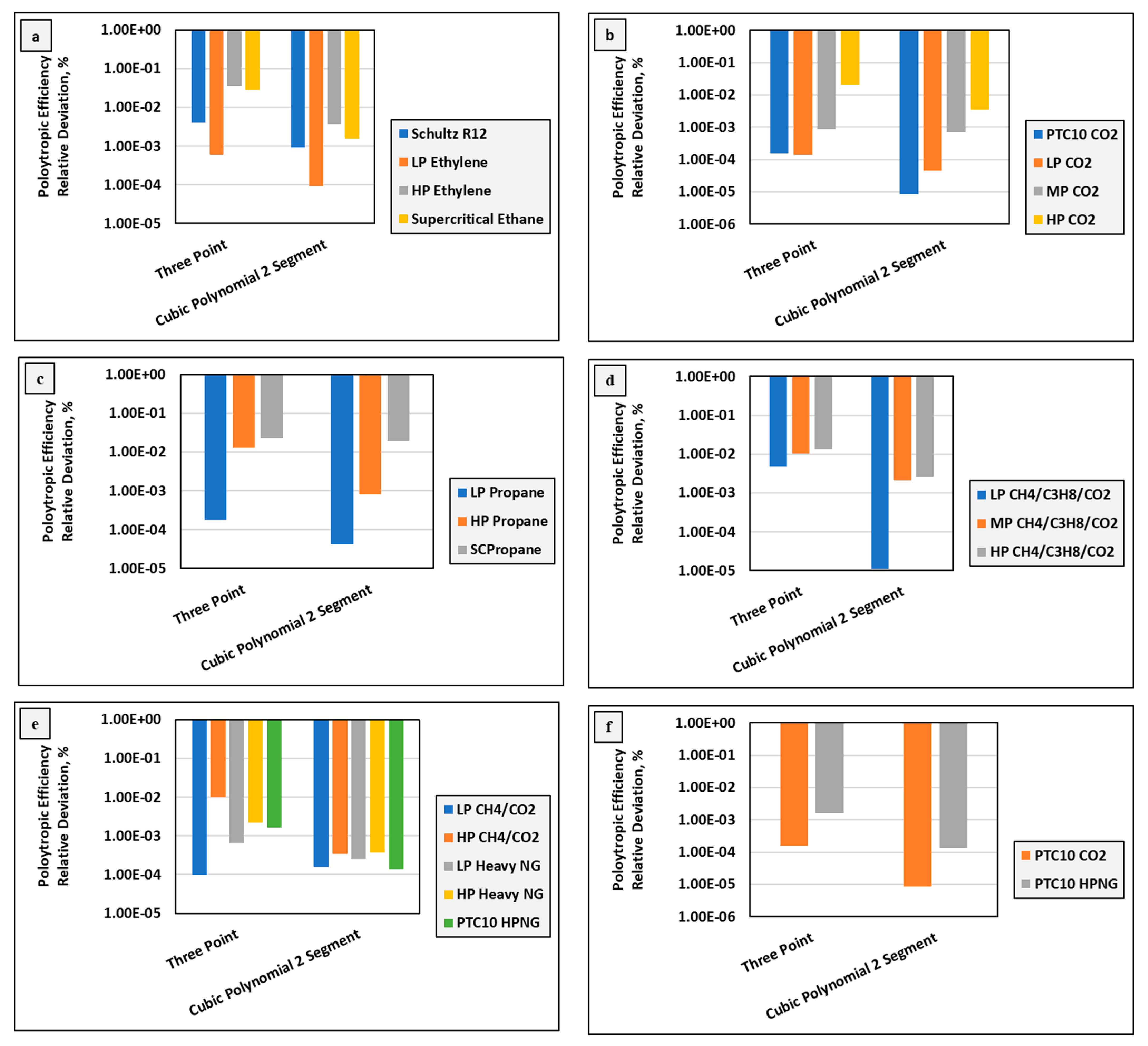
- Cubic polynomial sequential segment path methods were demonstrated to achieve high accuracy acceptable polytropic efficiency results significantly faster with fewer segments required than linear polynomial path methods based upon 115 compression example cases.
- ○
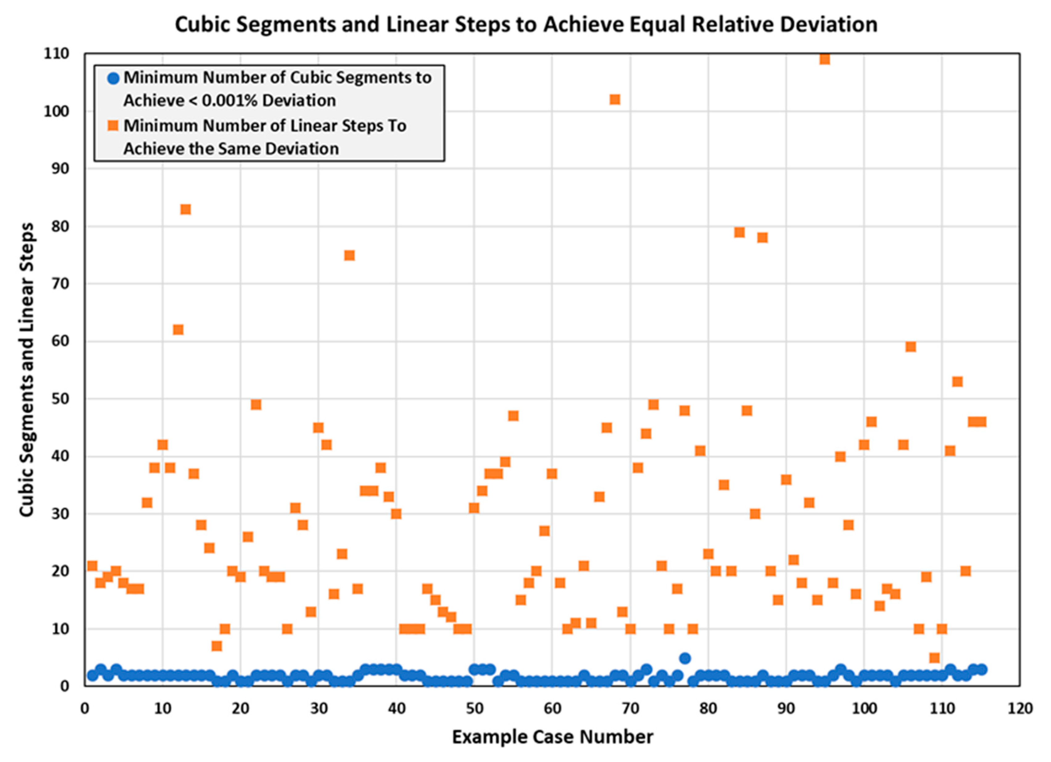
- For all 115 example cases, T-s polytropic paths agreed between 10 cubic segments and 100 linear steps which confirmed the validity of using the result of 10-segment cubic polynomial approximants as the standard for comparison for polytropic efficiency relative deviation and uncertainty.
- ○
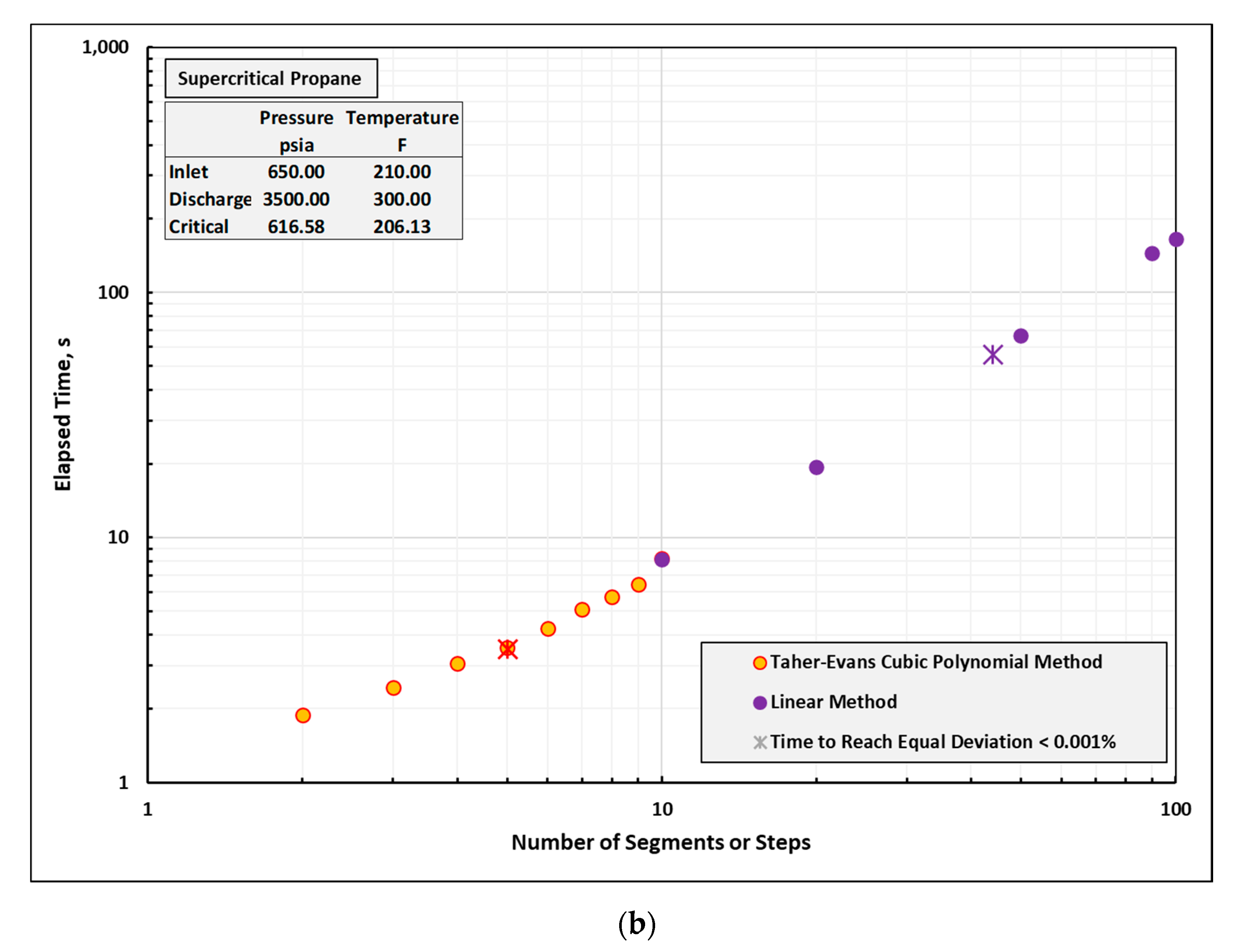
- Cubic polynomial path methods show that the required number of segments to achieve an acceptable result remains within a maximum of five segments or less for all the cases studied. For the linear polynomial path method, the required number of steps did not follow a regular pattern as shown in Figure 11. No rule or algorithm can be determined for the required number of linear polynomial steps to achieve an acceptable result.
- ○
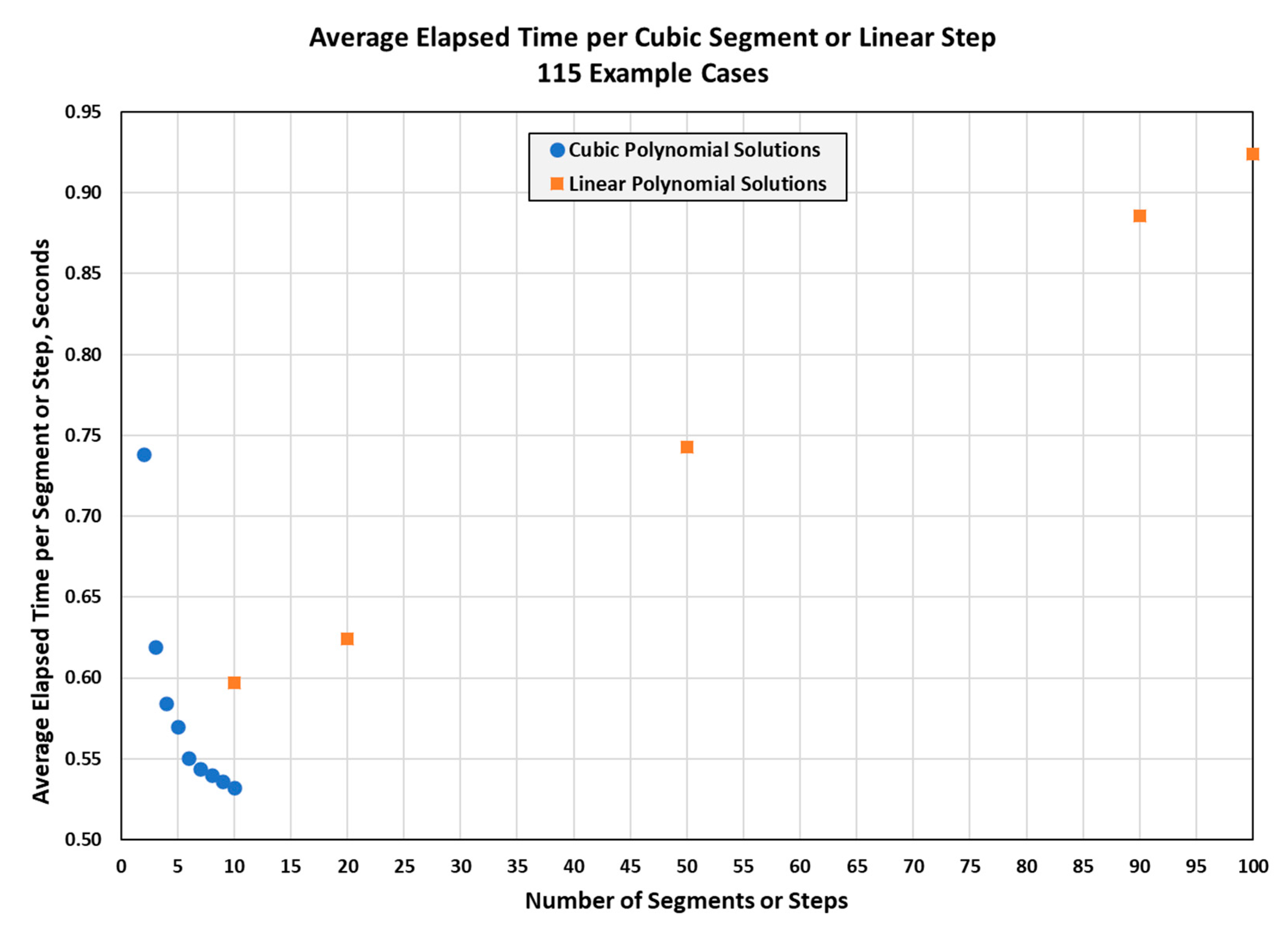
- While both cubic and linear polynomial methods can reach acceptable results, the cubic methods require fewer repetitive iterations and are completed much faster. Sequential segment cubic polynomial method calculations are typically at least an order of magnitude faster than sequential step linear polynomial methods. This is a clear advantage for cubic methods when processing compressor performance test data in real time.
- ○
- The cubic polynomial methods provide an order of magnitude lower uncertainty with significantly fewer cubic segments than linear polynomial methods. (See Figure A10).
- ○
- The cubic polynomial methods’ uncertainty rapidly decreases as the number of segments increases while the linear polynomial methods illustrate a much more gradual decrease in uncertainty as they approach an asymptote. The linear polynomial methods uncertainty asymptote appears to be more than an order of magnitude greater than the cubic methods.
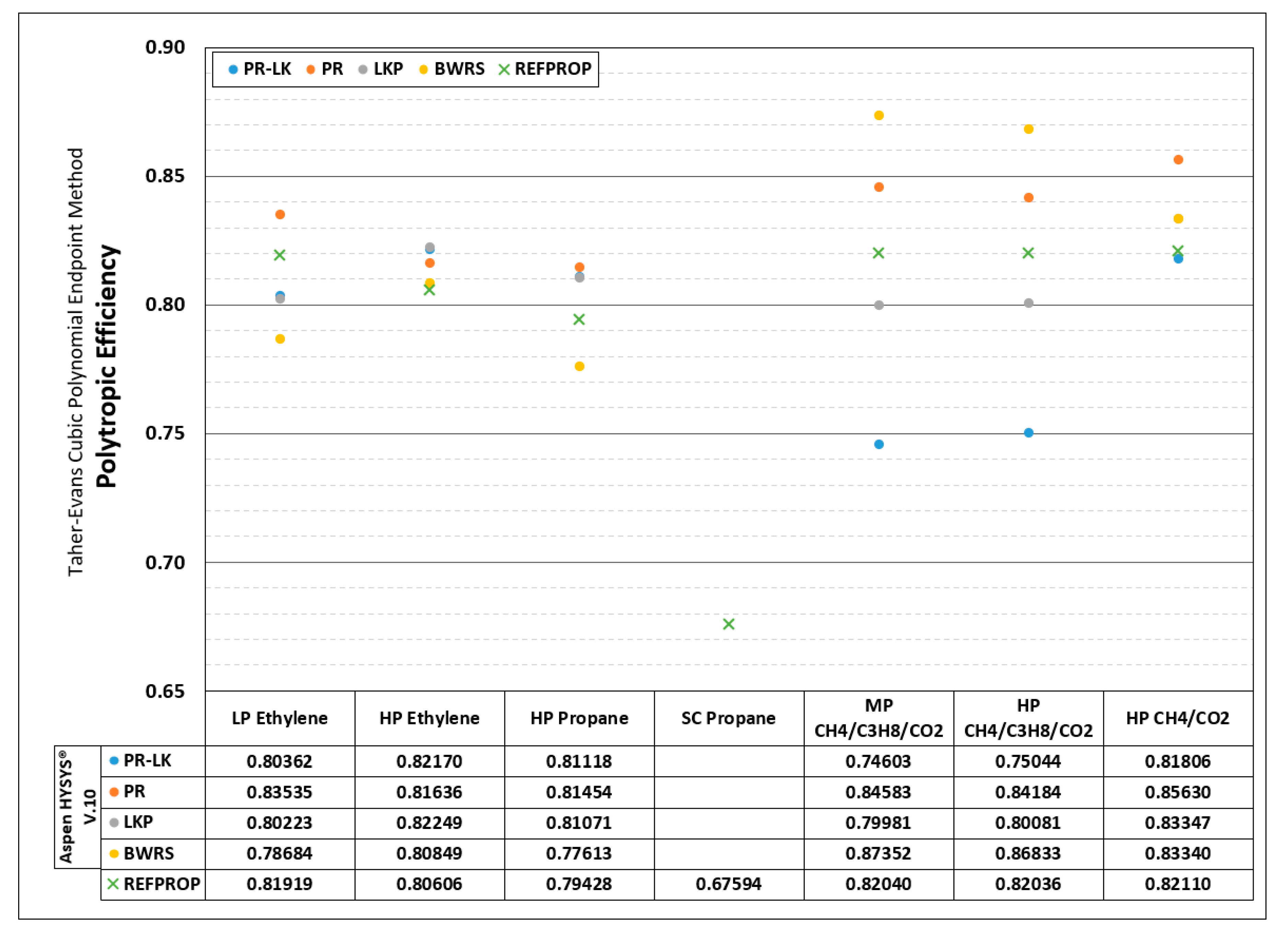
- Identical calculations for selected example cases using several different equations of state to obtain thermodynamic state point data for application of cubic and linear polynomial methods revealed significant differences in results for efficiency can occur based upon the chosen EOS. See Appendix D for selective examples.
- When rapid, highly accurate, low uncertainty, centrifugal compressor polytropic efficiency calculations are required, the Taher–Evans Cubic Polynomial methods (TE-CP) should be used.
- Due to significant differences found between results when employing various equations of state, it is recommended that a project use the same equation of state throughout the project timeline to avoid potential discrepancies.
Author Contributions
Funding
Institutional Review Board Statement
Informed Consent Statement
Data Availability Statement
Conflicts of Interest
Nomenclature
| A | Polynomial approximant coefficient |
| B | Polynomial approximant coefficient |
| b | Linear approximant coefficient |
| Isobaric expansivity, | |
| BWRS | Benedict–Webb–Rubin EOS as modified by K. E. Starling |
| C | Polynomial approximant coefficient |
| CH4 | Methane |
| CO2 | Carbon Dioxide |
| C3H8 | Propane |
| CP | Cubic Polynomial |
| Cp | heat capacity at constant pressure |
| D | Polynomial approximant coefficient |
| E | Slope of the polytropic path on the T-s diagram, |
| EOS | Equation of State |
| Deviation of polytropic efficiency | |
| Deviation of approximated temperature | |
| Deviation of approximated | |
| EOS | Equation of State |
| h | Specific enthalpy |
| HP | High pressure |
| OEM | Original Equipment Manufacturer |
| PR | Peng-Robinson EOS |
| PR-LKP | Peng-Robinson EOS and the Lee-Kesler EOS for the calculation of enthalpies |
| LP | Linear Polynomial, or Low Pressure |
| LKP | Lee-Kesler-Plöcker EOS |
| m | Linear approximant coefficient |
| MP | Medium Pressure |
| Schultz [6] polytropic volume exponent as applied in | |
| T | Temperature |
| TE-CP | Taher–Evans Cubic Polynomial |
| REFPROP | Reference properties EOS software |
| s | Specific entropy |
| SC | Supercritical |
| Specific volume | |
| Compressibility function, | |
| Schultz method using compressibility functions and | |
| Polytropic efficiency | |
| Subscripts and Superscripts | |
| indicates the ith segment | |
| total number of segments | |
| degree of the polynomial approximant Example: indicates the cubic polynomial approximant, which is used to approximate the segment number 6 of a polytropic path that is divided into 10 segments. This symbology provides a clear way to compare different methods discussed in this paper. | |
| inf | inflection |
| p | Polytropic, or pressure |
| r | ratio |
| d | compressor section discharge (measured) |
| 1 | compressor section inlet |
| 2 | compressor section discharge |
Appendix A. Temperature Change with Entropy along the Polytropic Path
Appendix B. Comparative Numeric Examples of Application of the Taher–Evans Cubic Polynomial Methods
- Endpoint methods
- Three point methods
- ○
- Cubic Polynomial two segment;
- ○
- Huntington’s three point [13].
- Multi-step and multi-segment methods
- ○
- Cubic Polynomial—sequential segments (2 through 10 segments);
- ○
- Linear Polynomial—sequential steps (10, 20, 50, 90 and 100 steps).

| Case Number | 1 | 2 | 3 | 4 | 5 | 6 | 7 | 8 | 9 | 10 | 11 | |
| Case Name | Schultz R12 | LP Ethylene | HP Ethylene | SC Ethane | PTC10 CO2 | LP CO2 | MP CO2 | HP CO2 | LP Propane | HP Propane | SC Propane | |
| Composition, mol % | Ethane | 1.0000 | ||||||||||
| Propane | 1.0000 | 1.0000 | 1.0000 | |||||||||
| Carbon Dioxide | 1.0000 | 1.0000 | 1.0000 | 1.0000 | ||||||||
| Ethylene | 1.0000 | 1.0000 | ||||||||||
| R12 | 1.0000 | |||||||||||
| Compression Conditions | , psia | 10 | 360 | 362.5 | 750 | 300.01 | 400 | 500 | 1100.1 | 17.99 | 300 | 650 |
| , bara | 0.689 | 24.821 | 24.993 | 51.710 | 20.685 | 27.579 | 34.474 | 75.849 | 1.240 | 20.684 | 44.816 | |
| , °F | −10 | 50 | 98.3 | 110 | 100 | 100 | 75 | 98.3 | −31.36 | 200 | 210 | |
| , °C | −23.33 | 10 | 36.833 | 43.333 | 37.778 | 37.778 | 23.88 | 36.833 | −35.2 | 93.333 | 98.889 | |
| , psia | 130 | 1000 | 7250 | 3500 | 487.76 | 1200 | 3000 | 6000.3 | 60 | 1000 | 3500 | |
| , bara | 8.963 | 68.948 | 499.870 | 241.316 | 33.630 | 82.737 | 206.843 | 413.706 | 4.137 | 68.948 | 241.316 | |
| , °F | 210 | 195 | 566.3 | 285 | 201.59 | 325 | 400 | 368.3 | 60 | 330 | 300 | |
| , °C | 98.889 | 90.556 | 296.833 | 140.556 | 94.217 | 162.778 | 204.444 | 186.833 | 15.556 | 165.556 | 148.889 | |
| Case Number | 12 | 13 | 14 | 15 | 16 | 17 | 18 | 19 | ||||
| Case Name | LP CH4/C3H8/CO2 | MP CH4/C3H8/CO2 | HP CH4/C3H8/CO2 | LP CH4/CO2 | HP CH4/CO2 | LP Heavy NG | HP Heavy NG | PTC10 HPNG | ||||
| Composition, mol % | Methane | 0.30294 | 0.30294 | 0.30294 | 0.256274 | 0.256274 | 0.688671 | 0.688671 | 0.8600 | |||
| Ethane | 0.03748 | 0.03748 | 0.03748 | 0.022871 | 0.022871 | 0.119957 | 0.119957 | 0.1125 | ||||
| Propane | 0.43533 | 0.43533 | 0.43533 | 0.005691 | 0.005691 | 0.102964 | 0.102964 | 0.0075 | ||||
| isoButane | 0.00222 | 0.00222 | 0.00222 | 0.000001 | 0.000001 | 0.031432 | 0.031432 | |||||
| Butane | 0.00218 | 0.00218 | 0.00218 | 0.000001 | 0.000001 | 0.027541 | 0.027541 | |||||
| isoPentane | 0.000001 | 0.000001 | 0.008927 | 0.008927 | ||||||||
| Pentane | 0.000001 | 0.000001 | 0.005563 | 0.005563 | ||||||||
| Hexane | 0.000175 | 0.000175 | ||||||||||
| Nitrogen | 0.00399 | 0.00399 | 0.00399 | 0.002629 | 0.002629 | 0.002477 | 0.002477 | 0.0040 | ||||
| Carbon Dioxide | 0.21586 | 0.21586 | 0.21586 | 0.712356 | 0.712356 | 0.012468 | 0.012468 | 0.0160 | ||||
| Compression Conditions | , psia | 650 | 2071 | 2071 | 500 | 1649.7 | 500 | 1750 | 2520.6 | |||
| , bara | 44.816 | 142.790 | 142.790 | 34.474 | 113.743 | 34.474 | 120.658 | 173.789 | ||||
| , °F | 115 | 160 | 160 | 50 | 101.2 | 100 | 50 | 100 | ||||
| , °C | 46.111 | 71.111 | 71.111 | 10 | 38.444 | 37.778 | 10 | 37.778 | ||||
| , psia | 2200 | 10,025.70 | 11,010.80 | 1700 | 8189.70 | 1800 | 4375 | 6500 | ||||
| , bara | 151.685 | 691.248 | 759.168 | 117.211 | 564.660 | 124.106 | 301.646 | 448.159 | ||||
| , °F | 270 | 291.9 | 301.5 | 250 | 316.2 | 295 | 125 | 280 | ||||
Appendix B.1. Endpoint Methods
- Schulz—with based upon the endpoints of compression
- ○
- Schultz average n—with averaged based upon individual calculations at inlet and discharge
- ○
- ○
- HP ethylene; Mallen and Saville [9] highlighted their improvements over Schultz’s method for high pressure, but still have an approximate 1% deviation;
- ○
- LP and HP ethylene; typical and expected patterns for cubic and linear polynomials.
- Figure A1b,c
- ○
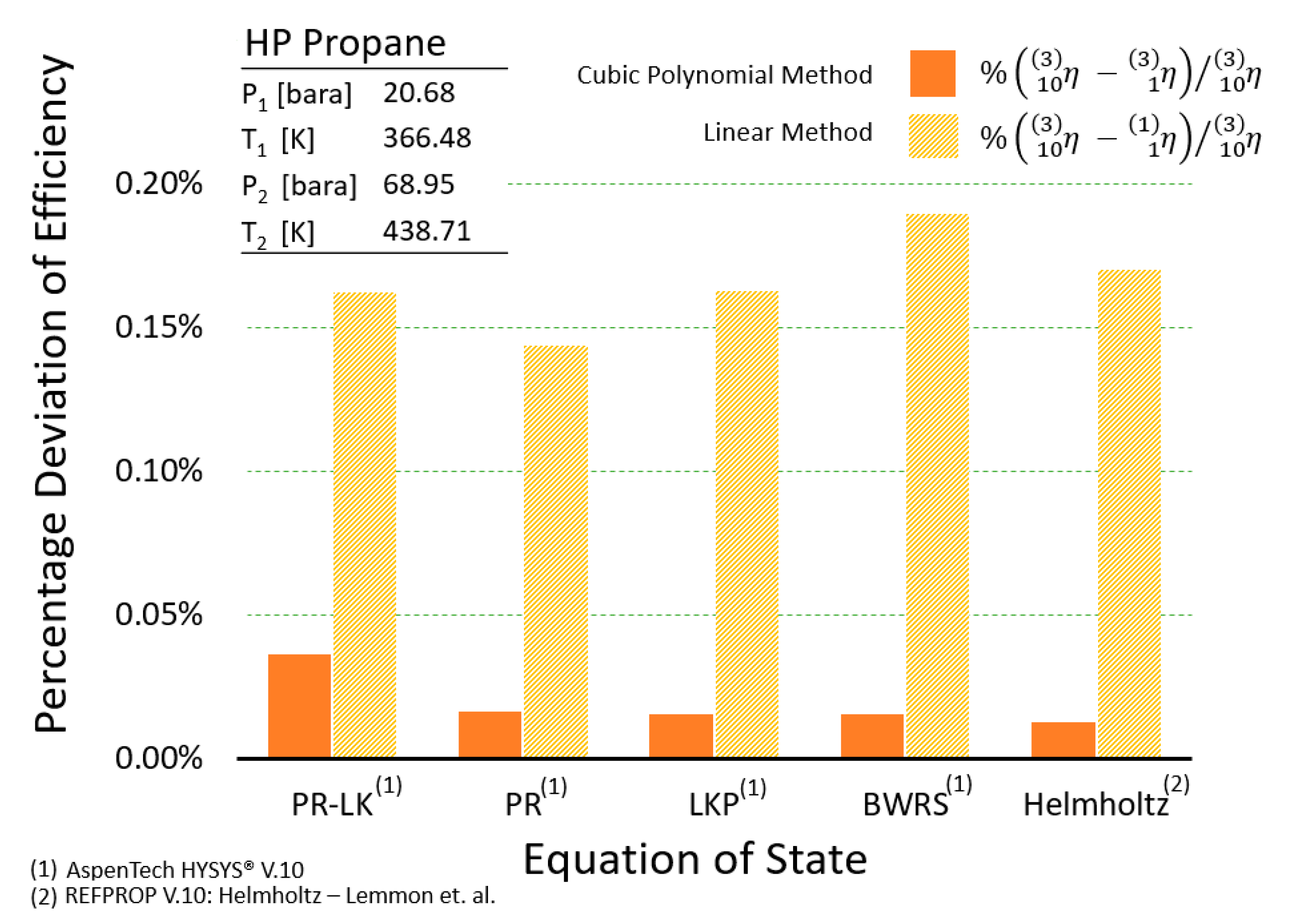
- CO2 and propane; as pressure increases accuracy decreases is a typical pattern
- ○
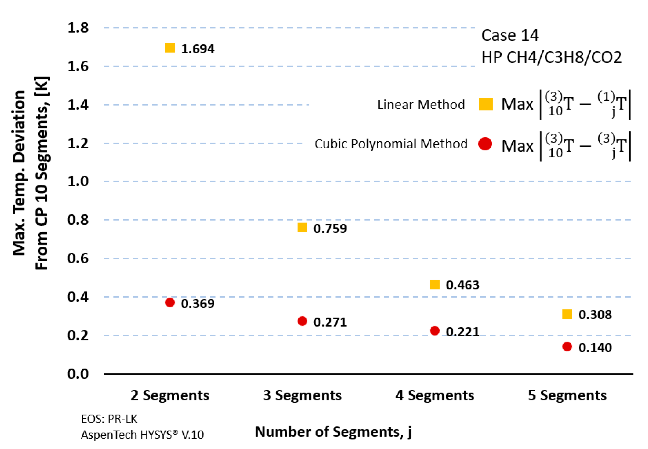
- CH4/C3H8/CO2; medium and high pressure cases are very similar since discharge conditions are close
- ○
- PTC10; the HPNG case will require more cubic segments to achieve sufficient accuracy than the Type 2 test design using CO2

| Case Number | Case 1 | Case 2 | Case 3 | Case 4 | Case 5 |
| T-s Slope at Inlet, , lbm.R2/BTU | 14,168 | 10,442 | 9383 | 14,537 | 7026 |
| T-s Slope at Discharge, , lbm.R2/BTU | 19,822 | 12,253 | 8302 | 7946 | 7881 |
| T-s Slope Change, % | 39.90 | 17.34 | −11.52 | −45.34 | 12.17 |
| T-s Curve Shape Category | I | I | III | II | I |
| Entropy at Inflection Point, BTU/lbm.R | - | - | 0.65070 | - | - |
| Temperature at Inflection Point, °F | - | - | 304.71 | - | - |
| Case Number | Case 6 | Case 7 | Case 8 | Case 9 | Case 10 |
| T-s Slope at Inlet, , lbm.R2/BTU | 8551 | 15,181 | 10,553 | 7178 | 10,330 |
| T-s Slope at Discharge, , lbm.R2/BTU | 10,744 | 19,708 | 8887 | 8151 | 15,523 |
| T-s Slope Change, % | 25.66 | 29.82 | −15.79 | 13.57 | 50.28 |
| T-s Curve Shape Category | I | I | II | I | I |
| Entropy at Inflection Point, BTU/lbm.R | - | - | - | - | - |
| Temperature at Inflection Point, °F | - | - | - | - | - |
| Case Number | Case 11 | Case 12 | Case 13 | Case 14 | Case 15 |
| T-s Slope at Inlet, , lbm.R2/BTU | 14,053 | 10,664 | 11,513 | 11,509 | 13,135 |
| T-s Slope at Discharge, , lbm.R2/BTU | 3773 | 9986 | 5526 | 5352 | 16,183 |
| T-s Slope Change, % | −73.15 | −6.36 | −52.01 | −53.50 | 23.20 |
| T-s Curve Shape Category | III | III | III | III | I |
| Entropy at Inflection Point, BTU/lbm.R | 0.48820 | 0.64410 | 0.55540 | 0.55670 | - |
| Temperature at Inflection Point, °F | 288.95 | 176.68 | 286.75 | 294.07 | - |
| Case Number | Case 16 | Case 17 | Case 18 | Case 19 | |
| T-s Slope at Inlet, , lbm.R2/BTU | 18,783 | 5147 | 4601 | 2786 | |
| T-s Slope at Discharge, , lbm.R2/BTU | 12,049 | 5762 | 3362 | 2632 | |
| T-s Slope Change, % | −35.85 | 11.94 | −26.94 | −5.53 | |
| T-s Curve Shape Category | II | I | II | II | |
| Entropy at Inflection Point, BTU/lbm.R | - | - | - | - | |
| Temperature at Inflection Point, °F | - | - | - | - |
Appendix B.2. Three Point Methods

Appendix B.3. Multi-Step and Multi-Segment Methods
| Case Number | Case 1 | Case 2 | Case 3 | Case 4 | Case 5 | Case 6 | Case 7 |
|---|---|---|---|---|---|---|---|
| Cubic Polynomial 2 Segment | 75.0442 | 81.9199 | 80.6174 | 79.9531 | 59.4118 | 65.2211 | 78.4933 |
| Cubic Polynomial 3 Segment | 75.0437 | 81.9200 | 80.6148 | 79.9521 | 59.4118 | 65.2211 | 78.4938 |
| Cubic Polynomial 4 Segment | 75.0436 | 81.9200 | 80.6146 | 79.9519 | 59.4118 | 65.2211 | 78.4939 |
| Cubic Polynomial 5 Segment | 75.0435 | 81.9200 | 80.6145 | 79.9519 | 59.4118 | 65.2211 | 78.4939 |
| Cubic Polynomial 6 Segment | 75.0435 | 81.9200 | 80.6145 | 79.9519 | 59.4118 | 65.2211 | 78.4939 |
| Cubic Polynomial 7 Segment | 75.0435 | 81.9200 | 80.6145 | 79.9519 | 59.4118 | 65.2211 | 78.4939 |
| Cubic Polynomial 8 Segment | 75.0435 | 81.9200 | 80.6145 | 79.9519 | 59.4118 | 65.2211 | 78.4939 |
| Cubic Polynomial 9 Segment | 75.0435 | 81.9200 | 80.6145 | 79.9519 | 59.4118 | 65.2211 | 78.4939 |
| Cubic Polynomial 10 Segment | 75.0435 | 81.9200 | 80.6145 | 79.9519 | 59.4118 | 65.2211 | 78.4939 |
| Linear Polynomial 10 step | 75.0408 | 81.9194 | 80.6153 | 79.9544 | 59.4111 | 65.2189 | 78.4916 |
| Linear Polynomial 20 step | 75.0428 | 81.9198 | 80.6147 | 79.9525 | 59.4116 | 65.2205 | 78.4933 |
| Linear Polynomial 50 step | 75.0434 | 81.9200 | 80.6145 | 79.9520 | 59.4118 | 65.2210 | 78.4938 |
| Linear Polynomial 90 step | 75.0435 | 81.9200 | 80.6145 | 79.9519 | 59.4118 | 65.2211 | 78.4939 |
| Linear Polynomial 100 step | 75.0435 | 81.9200 | 80.6145 | 79.9519 | 59.4118 | 65.2211 | 78.4939 |
| Case Number | Case 8 | Case 9 | Case 10 | Case 11 | Case 12 | Case 13 | Case 14 |
| Cubic Polynomial 2 Segment | 64.3513 | 81.0248 | 79.4381 | 67.7882 | 76.7610 | 82.0678 | 82.0695 |
| Cubic Polynomial 3 Segment | 64.3497 | 81.0247 | 79.4386 | 67.7984 | 76.7610 | 82.0692 | 82.0712 |
| Cubic Polynomial 4 Segment | 64.3493 | 81.0247 | 79.4387 | 67.8002 | 76.7610 | 82.0694 | 82.0714 |
| Cubic Polynomial 5 Segment | 64.3492 | 81.0247 | 79.4387 | 67.8007 | 76.7610 | 82.0695 | 82.0715 |
| Cubic Polynomial 6 Segment | 64.3491 | 81.0247 | 79.4387 | 67.8009 | 76.7610 | 82.0695 | 82.0715 |
| Cubic Polynomial 7 Segment | 64.3491 | 81.0247 | 79.4387 | 67.8010 | 76.7610 | 82.0695 | 82.0716 |
| Cubic Polynomial 8 Segment | 64.3491 | 81.0247 | 79.4387 | 67.8010 | 76.7610 | 82.0695 | 82.0716 |
| Cubic Polynomial 9 Segment | 64.3491 | 81.0247 | 79.4387 | 67.8011 | 76.7610 | 82.0695 | 82.0716 |
| Cubic Polynomial 10 Segment | 64.3491 | 81.0247 | 79.4387 | 67.8011 | 76.7610 | 82.0695 | 82.0716 |
| Linear Polynomial 10 step | 64.3512 | 81.0243 | 79.4375 | 67.8050 | 76.7612 | 82.0715 | 82.0738 |
| Linear Polynomial 20 step | 64.3496 | 81.0246 | 79.4384 | 67.8021 | 76.7610 | 82.0700 | 82.0721 |
| Linear Polynomial 50 step | 64.3491 | 81.0247 | 79.4387 | 67.8013 | 76.7610 | 82.0696 | 82.0717 |
| Linear Polynomial 90 step | 64.3491 | 81.0247 | 79.4387 | 67.8012 | 76.7610 | 82.0695 | 82.0716 |
| Linear Polynomial 100 step | 64.3491 | 81.0247 | 79.4387 | 67.8011 | 76.7610 | 82.0695 | 82.0716 |
| Case Number | Case 15 | Case 16 | Case 17 | Case 18 | Case 19 | ||
| Cubic Polynomial 2 Segment | 80.3316 | 82.1055 | 72.1215 | 71.3151 | 59.2985 | ||
| Cubic Polynomial 3 Segment | 80.3317 | 82.1052 | 72.1216 | 71.3153 | 59.2984 | ||
| Cubic Polynomial 4 Segment | 80.3317 | 82.1052 | 72.1217 | 71.3154 | 59.2984 | ||
| Cubic Polynomial 5 Segment | 80.3317 | 82.1052 | 72.1217 | 71.3154 | 59.2984 | ||
| Cubic Polynomial 6 Segment | 80.3317 | 82.1052 | 72.1217 | 71.3154 | 59.2984 | ||
| Cubic Polynomial 7 Segment | 80.3317 | 82.1052 | 72.1217 | 71.3154 | 59.2984 | ||
| Cubic Polynomial 8 Segment | 80.3317 | 82.1052 | 72.1217 | 71.3154 | 59.2984 | ||
| Cubic Polynomial 9 Segment | 80.3317 | 82.1052 | 72.1217 | 71.3154 | 59.2984 | ||
| Cubic Polynomial 10 Segment | 80.3317 | 82.1052 | 72.1217 | 71.3154 | 59.2984 | ||
| Linear Polynomial 10 step | 80.3306 | 82.1073 | 72.1209 | 71.3164 | 59.2990 | ||
| Linear Polynomial 20 step | 80.3315 | 82.1057 | 72.1215 | 71.3156 | 59.2986 | ||
| Linear Polynomial 50 step | 80.3317 | 82.1053 | 72.1216 | 71.3154 | 59.2984 | ||
| Linear Polynomial 90 step | 80.3317 | 82.1052 | 72.1217 | 71.3154 | 59.2984 | ||
| Linear Polynomial 100 step | 80.3317 | 82.1052 | 72.1217 | 71.3154 | 59.2984 |


Appendix B.4. High Pressure Ethylene Example


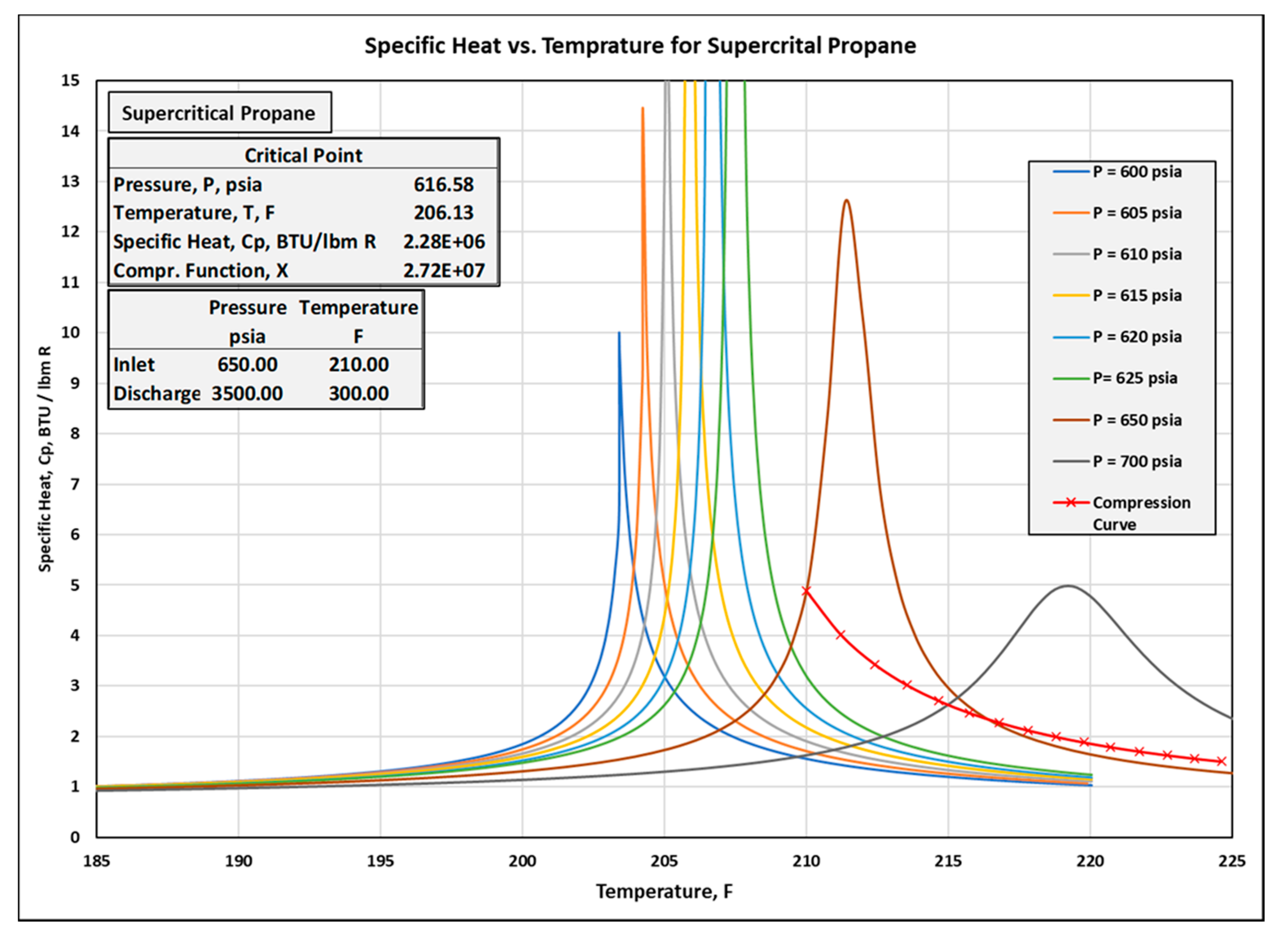
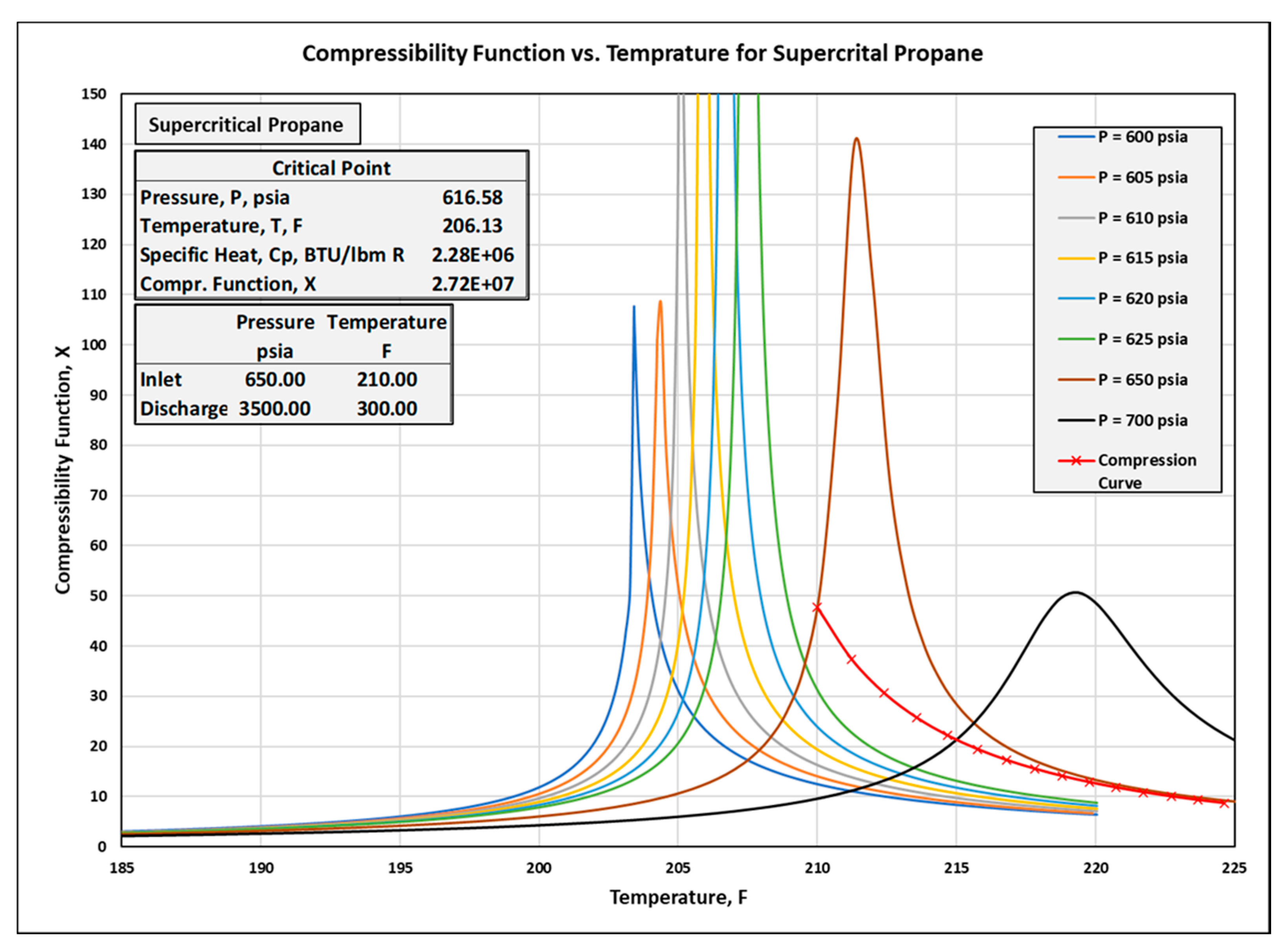
Appendix B.5. Supercritical Propane Example


Appendix C. Overview of 115 Example Case Results

- Category I: 3 cubic polynomial segments required;
- Category II: 5 cubic polynomial segments required;
- Category III: 5 cubic polynomial segments required.
| T-s Path Category | Number of Cubic Polynomial Segments Required | Totals | ||||
|---|---|---|---|---|---|---|
| 1 Segment | 2 Segments | 3 Segments | 4 Segments | 5 Segments | ||
| I | 28 | 16 | 44 | |||
| II | 10 | 28 | 8 | 1 | 47 | |
| III | 4 | 13 | 7 | 24 | ||
| Totals | 42 | 57 | 15 | 0 | 1 | 115 |


Appendix D. Equation of State Impact on Polytropic Efficiency
- Enthalpy, ;
- Entropy, ;
- Specific heat at constant pressure, ;
- Compressibility function, .
- PR, Peng–Robinson [30];
- PR-LK, Peng–Robinson with Lee–Kesler Enthalpy;
- ○
- Employs individual, reference quality EOS for each pure fluid;
- ○
- Applies mixing rules to the Helmholtz energy of the mixture components;
- ○
- REFPROP is a program, not a database of measurements.

References
- Taher, M. Mathematical Modeling of the Polytropic Process Using the Sequential Cubic Polynomial Approximation. In Proceedings of the ASME GT2021, ASME Turbo Expo 2021, Virtual, Online, 7–11 June 2021. Paper Number GT2021-59715. [Google Scholar]
- Taher, M.; Evans, B.F. Centrifugal Compressor Polytropic Performance Evaluation Using Cubic Polynomial Approximation for the Temperature-Entropy Polytropic Path. In Proceedings of the ASME GT2021, ASME Turbo Expo 2021, Virtual, Online, 7–11 June 2021. Paper Number GT2021-59678. [Google Scholar]
- Evans, B.F. Centrifugal Compressor Polytropic Efficiency—Cubic and Linear Polynomial Solution Methods Comparing 115 Example Case Calculations; Technology Report; ResearchGate: Berlin, Germany, 2020. [Google Scholar] [CrossRef]
- ASME PTC 10. Performance Test Code on Compressors and Exhausters; American Society of Mechanical Engineers: New York, NY, USA, 1997. [Google Scholar]
- Zeuner, G.A. Fundamental Laws of Thermodynamics Theory of Gases. In Technical Thermodynamics; D. Van Nostrand Company: New York, NY, USA, 1906; Volume 1. [Google Scholar]
- Schultz, J.M. The Polytropic Analysis of Centrifugal Compressors. ASME J. Eng. Power 1962, 84, 69–82. [Google Scholar] [CrossRef]
- ASME PTC 10. Compressors and Exhausters Power Test Code 10; American Society of Mechanical Engineers: New York, NY, USA, 1965. [Google Scholar]
- ASME PTC 10. Compressors and Exhausters Power Test Code 10; reaffirmed of the 1965 edition; American Society of Mechanical Engineers: New York, NY, USA, 1992. [Google Scholar]
- Mallen, M.; Saville, G. Polytropic Processes in the Performance Prediction of Centrifugal Compressors; Institution of Mechanical Engineers Conference Publications C183/77; Institution of Mechanical Engineers: London, UK, 1977; pp. 89–96. [Google Scholar]
- Kent, R.G. Application of Basic Thermodynamics to Compressor Cycle Analysis. In Proceedings of the International Compressor Engineering Conference, West Lafayette, IN, USA, 10–12 July 1974. Paper 135. [Google Scholar]
- Nathoo, N.S.; Gottenberg, W.G. Measuring the Thermodynamic Performance of Multistage Compressors Operating on Mixed Hydrocarbon Gases. In Proceedings of the Tenth Turbomachinery Symposium; Turbomachinery Laboratory, Texas A&M University: College Station, TX, USA, 1981; pp. 15–23. [Google Scholar]
- Nathoo, N.S.; Gottenberg, W.G. A New Look at Performance Analysis of Centrifugal Compressors Operating with Mixed Hydrocarbon Gases. ASME J. Eng. Power 1983, 105, 920–926. [Google Scholar] [CrossRef]
- Huntington, R.A. Evaluation of Polytropic Calculation Methods for Turbomachinery Performance. ASME Trans. J. Eng. Gas Turbines Power 1985, 107, 872–879. [Google Scholar] [CrossRef]
- Huntington, R. Limitations of the Schultz Calculation for Polytropic Head—A Proposal for Revision of PTC-10; Technology Report; ResearchGate: Berlin, Germany, 1997. [Google Scholar] [CrossRef]
- Hundseid, O.; Bakken, L.E.; Helde, T. A Revised Compressor Polytropic Performance Analysis. In Proceedings of the ASME GT2006, ASME Turbo Expo 2006, Barcelona, Spain, 8–11 May 2006. Paper Number 91033. [Google Scholar]
- Oldrich, J. Advanced Polytropic Calculation Method of Centrifugal Compressor. In Proceedings of the ASME IMECE2010, the ASME International Mechanical Engineering Congress and Exposition 2010, Vancouver, BC, Canada, 12–18 November 2010. Paper Number 40931. [Google Scholar]
- Sandberg, M.R.; Colby, G.M. Limitations of ASME PTC 10 in Accurately Evaluating Centrifugal Compressor Thermodynamic Performance. In Proceedings of the 42nd Turbomachinery Symposium, Houston, TX, USA, 1–3 October 2013; Turbomachinery Laboratory, Texas A&M University: College Station, TX, USA, 2013. [Google Scholar]
- Taher, M. ASME PTC-10 Performance Testing of Centrifugal Compressors—The Real Gas Calculation Method. In Proceedings of the ASME GT2014, ASME Turbo Expo 2014, Düsseldorf, Germany, 16–20 June 2014. Paper Number GT2014-26411. [Google Scholar]
- Wettstein, H.E. Polytropic Change of State Calculations. In Proceedings of the ASME IMECE2014, the ASME International Mechanical Engineering Congress and Exposition 2014, Montreal, QC, Canada, 14–20 November 2014. Paper Number 36202. [Google Scholar]
- Plano, M. Evaluation of Thermodynamic Models used for Wet Gas Compressor Design. Master’s Thesis, Innovative Sustainable Energy Engineering, Norwegian University of Science and Technology, Trondheim, Norway, June 2014. [Google Scholar]
- Evans, B.F.; Huble, S.R. Centrifugal Compressor Polytropic Performance: Consistently Accurate Results from Improved Real Gas Calculations. In Proceedings of the ASME GT2017, ASME Turbo Expo 2017, Charlotte, NC, USA, 26–30 June 2017. Paper Number GT2017-65235. [Google Scholar]
- Evans, B.F.; Huble, S.R. Tutorial, ‘Centrifugal Compressor Performance: Making Enlightened Analysis Decisions. In Proceedings of the 46th Turbomachinery Symposium, Houston, TX, USA, 11–14 December 2017; Turbomachinery Laboratory, Texas A&M University: College Station, TX, USA, 2017. [Google Scholar]
- Sandberg, M.R. A More Detailed Explanation of the Sandberg-Colby Method for the Evaluation of Centrifugal Compressor Thermodynamic Performance; ResearchGate: Berlin, Germany, 2020. [Google Scholar] [CrossRef]
- Box, G.E.; Draper, N.R. Empirical Model-Building and Response Surfaces; Wiley: Hoboken, NJ, USA, 1987. [Google Scholar]
- IEEE/ASTM SI 10-2016—American National Standard for Metric Practice; Institute of Electrical and Electronics Engineers: Washington, DC, USA, 2016.
- Stepanoff, A.J. Turboblowers: Theory, Design, and Application of Centrifugal and Axial Flow Compressors and Fans; John Wiley and Sons: New York, NY, USA, 1955. [Google Scholar]
- HYSYS; Aspentech: Bedford, MA, USA, 2020.
- Lemmon, E.W.; Bell, I.H.; Huber, M.L.; McLinden, M.O. NIST Standard Reference Database 23: Reference Fluid Thermodynamic and Transport Properties-REFPROP, Version 10.0; Standard Reference Data Program; National Institute of Standards and Technology: Gaithersburg, MD, USA, 2018.
- Brown, R.N. Compressors Selection and Sizing, 2nd ed.; Butterworth-Heinemann: Woburn, MA, USA, 1997. [Google Scholar]
- Peng, D.Y.; Robinson, D.B. A New Two-Constant Equation of State. Ind. Eng. Chem. Fundam. 1976, 15, 59–64. [Google Scholar] [CrossRef]
- Lee, B.I.; Kesler, M.G. A Generalized Thermodynamic Correlation Based on Three-Parameter Corresponding States. AIChE J. 1975, 21, 510–527. [Google Scholar] [CrossRef]
- Plöcker, U.; Knapp, H.; Prausnitz, J. Calculation of High-Pressure Vapor-Liquid Equilibria from a Corresponding States Correlation with Emphasis on Asymmetric Mixtures. Ind. Chem. Process Des. Dev. 1978, 17, 324–332. [Google Scholar] [CrossRef]
- Benedict, M.; Webb, G.B.; Rubin, L.C. An Empirical Equation for Thermodynamic Properties of Light Hydrocarbons and their Mixtures. J. Chem. Phys. 1940, 8, 334–345. [Google Scholar] [CrossRef]
- Benedict, M.; Webb, G.B.; Rubin, L.C. An Empirical Equation for Thermodynamic Properties of Light Hydrocarbons and their Mixtures II. Mixtures of Methane, Ethane, Propane, and n-Butane. J. Chem. Phys. 1942, 10, 757–758. [Google Scholar] [CrossRef]
- Starling, K.E. Fluid Thermodynamic Properties for Light Petroleum Systems; Gulf Publishing: Houston, TX, USA, 1973. [Google Scholar]
- Span, R. Multiparameter Equations of State: An Accurate Source of Thermodynamic Property Data; Springer: New York, NY, USA, 2000. [Google Scholar]
- Span, R.; Wagner, W. A New Equation of State for Carbon Dioxide Covering the Fluid Region from the Triple-Point Temperature to 1100 K at Pressures up to 800 MPa. J. Phys. Chem. Ref. Data 1996, 25, 1509–1596. [Google Scholar] [CrossRef]


| Segment Number | ||||||||||||||
|---|---|---|---|---|---|---|---|---|---|---|---|---|---|---|
| [K] | [bar] | [kj/kg-K] | [kj/kg] | - | - | - | - | [kg-K2/kj] | [kg-K2/kj] | - | [kj/kg] | [kj/kg] | ||
| 1 | Inlet | 366.483 | 3.390 | 20.684 | −2276.711 | −184,369 | 1,886,535 | −6,432,843 | 7,310,148 | 1499 | 1650 | 0.81147 | 13.28549 | 3.08654 |
| Outlet | 379.567 | 3.398 | 26.316 | −2260.339 | ||||||||||
| 2 | Inlet | 379.567 | 3.398 | 26.316 | −2260.339 | 151,457 | −1,534,519 | 5,183,886 | −5,838,652 | 1650 | 1831 | 0.81147 | 13.19405 | 3.06530 |
| Outlet | 393.341 | 3.406 | 33.480 | −2244.080 | ||||||||||
| 3 | Inlet | 393.341 | 3.406 | 33.480 | −2244.080 | 86,118 | −868,526 | 2,921,119 | −3,276,023 | 1831 | 2020 | 0.81147 | 13.03013 | 3.02721 |
| Outlet | 407.879 | 3.414 | 42.596 | −2228.022 | ||||||||||
| 4 | Inlet | 407.879 | 3.414 | 42.596 | −2228.022 | −1,407,357 | 14,438,426 | −49,373,634 | 56,277,303 | 2020 | 2158 | 0.81147 | 12.82697 | 2.98001 |
| Outlet | 423.124 | 3.421 | 54.193 | −2212.215 | ||||||||||
| 5 | Inlet | 423.124 | 3.421 | 54.193 | −2212.215 | −4,606,378 | 47,325,393 | −162,069,532 | 185,004,389 | 2158 | 2187 | 0.81147 | 12.67478 | 2.94466 |
| Outlet | 438.706 | 3.428 | 68.948 | −2196.596 | ||||||||||
| Summary of all 5 Segments | 0.81147 | 65.01143 | 15.10372 | |||||||||||
Publisher’s Note: MDPI stays neutral with regard to jurisdictional claims in published maps and institutional affiliations. |
© 2021 by the authors. Licensee MDPI, Basel, Switzerland. This article is an open access article distributed under the terms and conditions of the Creative Commons Attribution (CC BY-NC-ND) license (https://creativecommons.org/licenses/by-nc-nd/4.0/).
Share and Cite
Taher, M.; Evans, F. Centrifugal Compressor Polytropic Performance—Improved Rapid Calculation Results—Cubic Polynomial Methods. Int. J. Turbomach. Propuls. Power 2021, 6, 15. https://doi.org/10.3390/ijtpp6020015
Taher M, Evans F. Centrifugal Compressor Polytropic Performance—Improved Rapid Calculation Results—Cubic Polynomial Methods. International Journal of Turbomachinery, Propulsion and Power. 2021; 6(2):15. https://doi.org/10.3390/ijtpp6020015
Chicago/Turabian StyleTaher, Matt, and Fred Evans. 2021. "Centrifugal Compressor Polytropic Performance—Improved Rapid Calculation Results—Cubic Polynomial Methods" International Journal of Turbomachinery, Propulsion and Power 6, no. 2: 15. https://doi.org/10.3390/ijtpp6020015
APA StyleTaher, M., & Evans, F. (2021). Centrifugal Compressor Polytropic Performance—Improved Rapid Calculation Results—Cubic Polynomial Methods. International Journal of Turbomachinery, Propulsion and Power, 6(2), 15. https://doi.org/10.3390/ijtpp6020015