1. Introduction
Measuring the unsteady flow downstream of turbomachinery rotors evolved from being a ‘niche’ research activity in the nineties to becoming a common practice the scientific studies of present-day turbomachinery [
1,
2,
3,
4,
5], with also relevant examples of industrial applications [
6,
7,
8]. Such evolution was supported by the technical development of instrumentation technology, of novel data-reduction methods, and by the practical experience of the experimentalists. A key contribution to this development came from one specific measurement technology, i.e., the Fast Response Aerodynamic Pressure Probe (FRAPP), which has undoubted advantages with respect to other intrusive or non-intrusive techniques in terms of rigidity, reliability, promptness. Last but not least, it provides total and static pressure measurements, which can be used for the evaluation of the blade-row and stage performance. Thanks to the very high temporal resolution, these probes also allowed to investigate experimentally the complex flow phenomena connected to unsteady blade row interaction [
9,
10,
11,
12,
13].
The FRAPP concept comes from the combination of fast-response pressure transducers, typically of the piezoresistive kind, with aerodynamic directional pressure probes. The transducers can be flush-mounted on the probe head [
14], enhancing the frequency response despite fragility; in other examples [
6,
15,
16,
17], the researchers preferred to embed the transducers within the probe head to enhance the probe strength. Excellent reviews on the early stages of FRAPP development can be found in [
18,
19,
20]. However, since then, further relevant improvements were made on the basic technology and some of them are reported in the very recent review proposed in [
21].
A specific version of FRAPP technology has been the object of research and development at Politecnico di Milano since 1998. The probe concept, that is alternative to those presented by the authors listed above, was first proposed in [
22], and further elaborated in [
23]. With the aim of minimizing the probe blockage while maximizing the instrumentation reliability, an optimal configuration was identified by using single- or two-sensor probes operated as virtual three- of four-sensor probes, and by adopting commercial transducers that only need to be mounted and glued within the probe head. This design implies the adoption of a relatively large line-cavity system connecting the pressure tap on the probe head to the sensor, strongly influencing the probe dynamic response. However, dedicated computational studies and the set-up of a novel dynamic calibration facility [
24] has ultimately led to the development of FRAPPs featuring a dynamic response of the order of 100 kHz after digital compensation with the experimental transfer function.
This paper proposes a review of the most relevant advances in FRAPP technology conceived and applied at Politecnico di Milano in the last decade, in terms of high-temperature applications, dynamic identification and uncertainty quantification, analyzing systematically probes for two-dimensional and three-dimensional measurements.
2. FRAPP Description
Before discussing technological aspects and metrological issues, this section proposes a review of the current probes’ shape configurations and their implication on the measurement capability. Two probes were considered, one cylindrical for two-dimensional flow measurements and one spherical for three-dimensional flow measurements. Even though the probes share several technical features, they are discussed separately in the following section.
2.1. Cylindrical Probe
The cylindrical shape makes the probe inherently suitable for measuring the flow direction in a plane normal to the cylinder axis (called the “yaw” angle in this paper), along with the total and static pressure. Conversely, it has a low sensitivity to the flow components parallel to the axis and hence, to the related flow angle, called the “pitch” in this paper, so that it can be considered insensitive for pitch angle values within ±10°, as resulted from a dedicated test campaign. As the probe embeds a single sensor for miniaturization, it needs three pressure readings measured at different rotations around the probe axis to virtually simulate the operation of a three-sensor probe. This prevents real-time unsteady measurements to be performed; however, unless operation instabilities are of concern, in case of unsteady turbomachinery flows, this is not a severe limitation as one is typically interested in the periodic component of the flow unsteadiness. The unsteady periodic component can be extracted by means of ensemble averages locked on the rotor wheel, using a key-phasor signal. The virtual operation prevents from achieving direct turbulence measurements, even if an estimate of the turbulence intensity is possible considering the signal acquired by the probe at the angular position aligned to the phase-averaged flow direction when the unresolved flow angle fluctuations are sufficiently low (±9°), as discussed in [
25].
As well visible in
Figure 1, which reports a drawing of the cylindrical FRAPP, the probe size and shape are determined by the sensor characteristics. The cylindrical shape was selected to miniaturize as much as possible the probe, thus reducing the probe blockage. The probe is, in practice, manufactured around one of the smallest transducers commercially available, which simply needs to be inserted within the cylinder and glued with a proper material. In this way, the size of the probe can be minimized down to about 2 mm. The smooth shape of the probe, combined with its miniaturization, guarantees optimal probe aerodynamics in terms of dynamic errors, according to dedicated studies performed at the early stages of FRAPP technology development [
26].
The probe design concept allows to deal with a relatively high temperature. Present-day piezoelectric transducers can operate up to about 550 K and epoxy resins are commercially available for temperatures greater than 600 K. The combination of these two elements allows manufacturing high-temperature FRAPP in a straightforward way and without external cooling—a topic that, however, has been the object of dedicated investigations [
27] that proved to be successful at the cost of an increase of probe blockage.
A further specific aspect of the present design is related to the installation of the sensor inside the probe head and to the subsequent line-cavity system connecting the pressure tap on the probe head to the sensor. The topic is discussed in detail in [
23], in which several analytical and numerical techniques are applied and compared to optimize the shape of the internal cavities in order to maximize the probe promptness. By virtue of this study, the promptness of the FRAPP resulted of about 80 kHz. Such value was—and still is—sufficiently high to match the specifications of all the FRAPP applications considered by the authors in their experience.
2.2. Spherical Probe
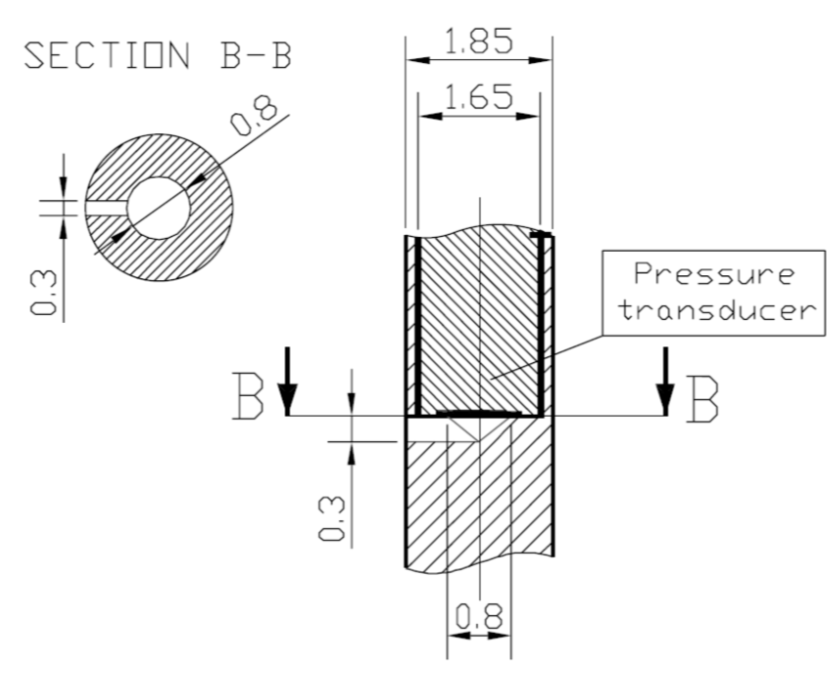
To overcome limitations in measurement capability of cylindrical probes, an alternative configuration suitable for unsteady 3D measurements was developed at Politecnico di Milano, featuring a spherical head shape and named sFRAPP.
In order to enhance the sensitivity to the flow components parallel to the probe axis, the probe head features a spherical shape with two pressure taps. The combination of the geometrical constraints imposed by the transducers as well as by the miniaturization of external and internal dimensions led to a head diameter of 3.8 mm and to a diameter of 0.3 mm for the two pneumatic lines feeding the cavities facing the sensors.
One pressure tap was drilled on the probe tip, with an inclination of 60° with respect to the probe axis, and it was employed only for measurement of the pitch angle. The second pressure tap was drilled on the equatorial plane with an inclination of 90° with respect to the probe axis: it can be aligned to the ‘pitch’ tap as shown in
Figure 2 or it can be rotated with respect to that by 180° around the probe stem.
A preliminary analysis of the sFRAPP is reported in [
28], and its first application downstream of a turbine stage is documented in [
29]. The probe operating mechanism is still based on multiple pressure readings taken at different rotations of the probe around its own stem: the combined use of four pressure readings allows to measure both the flow directions, alongside total and static pressure. The configuration shown in
Figure 2 allows reconstructing both the flow directions with just 3 rotations, while 4 rotations are required for the configuration with 2 opposed taps (a further rotation shifted by 180° with respect to the central one of the others). However, the use of opposed taps allows reducing the dimension of the internal cavities as, in this latter case, a shorter line connects the ‘pitch’ tap to the sensor. Theoretical estimates and experimental dynamic calibrations showed a reduction of promptness to 40 kHz, about half of the promptness of the sFRAPP with opposite taps, but still very high and fully suitable for typical turbomachinery applications.
3. Thermally Corrected Calibration of the Pressure Sensor
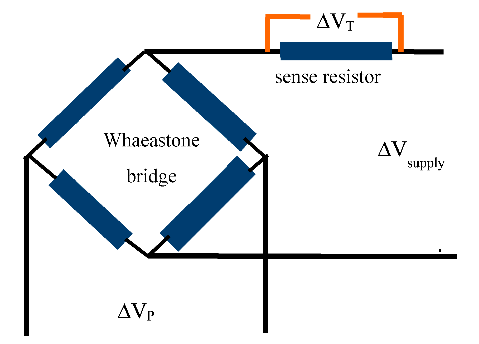
Due to the sensor sensitivity to the temperature, a sensor calibration in pressure and temperature is required before performing the aerodynamic and the dynamic ones. The sensor sensitivity to temperature is measured by applying an additional resistance (“sense resistor” in the following) on the bridge, as showed in
Figure 3. The voltage drop across the sense resistor (ΔV
T) is mainly a function of the current flowing across the bridge, which depends on the bridge temperature. Thus, by reading the voltage difference across the bridge (ΔV
P) and ΔV
T, the sensor behavior can be fully documented.
The probe temperature was set by inserting it in an oven: the insertion length was chosen to be representative of what is needed in the real application in order to minimize the effect of different thermal conductions along the stem.
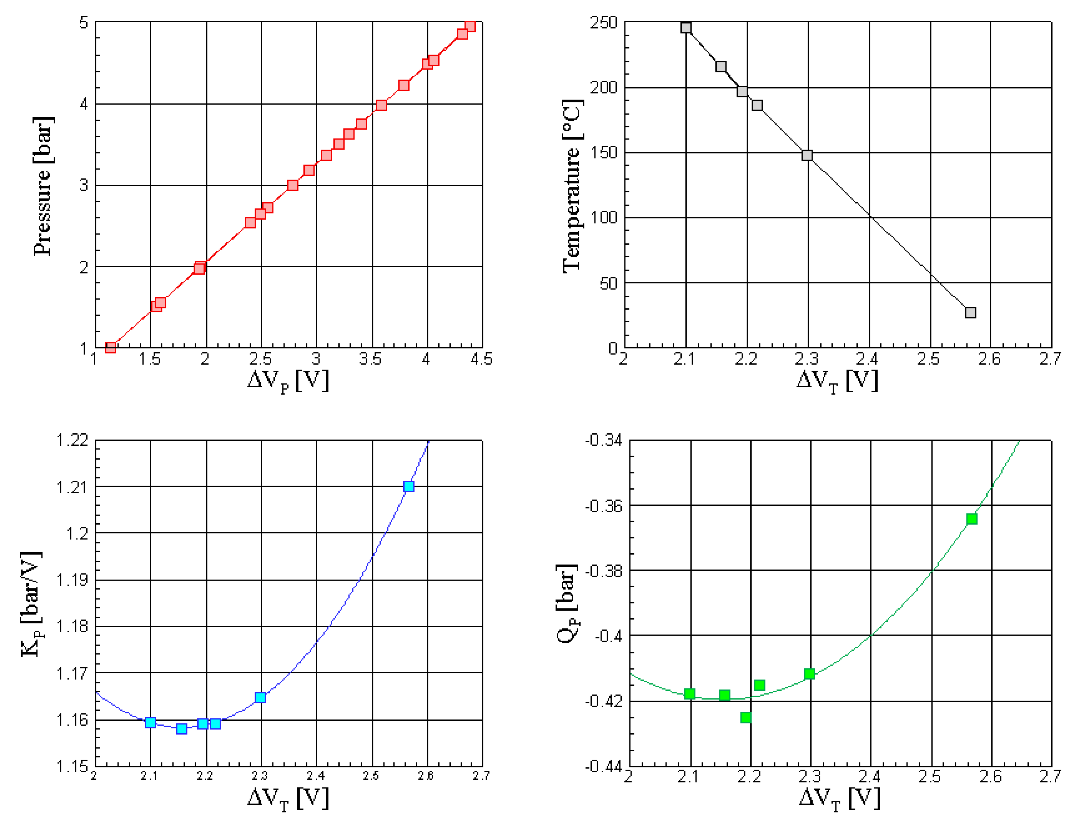
The calibration procedure was applied as follow: first, the oven temperature (Ti) was set and a consistent waiting time (typically 30 min) was scheduled to bring the probe to a steady thermal condition. Then, a pressure ramp was applied up to the calibration range foreseen for the tests. To include possible hysteretic behavior in the calibration coefficients and uncertainty, the pressure ramp had both positive and negative slopes. Then, the oven temperature was modified and the procedure repeated: also for the temperature ramp, positive and negative slopes could be applied.
For each temperature level (Ti), the pressure data were then fit by a linear function: the results show the slope (KP,i), intercept (QP,i) and uncertainty (UP,i).
K
P,i, Q
P,i, and U
P,i were then fit by polynomial functions (typically linear or parabolic, depending on the trend), to find the K
P and Q
P (as function of the ΔV
T). The sensor temperature Ti and ΔV
T,i could also be fitted to have K
T, Q
T.
Figure 4 shows typical calibration results.
The procedure is accurate and its only critical point is a random offset on QT,i due to the sensor thermal sensitivity while the KT,i is perfectly repeatable: this occurrence, whose magnitude unfortunately depends on the single transducer, requires an online check to measure it during tests.
Once K
T, Q
T, K
P, and Q
P are found, during the probe application, the sensor pressure (P) and temperature (T) can be calculated by
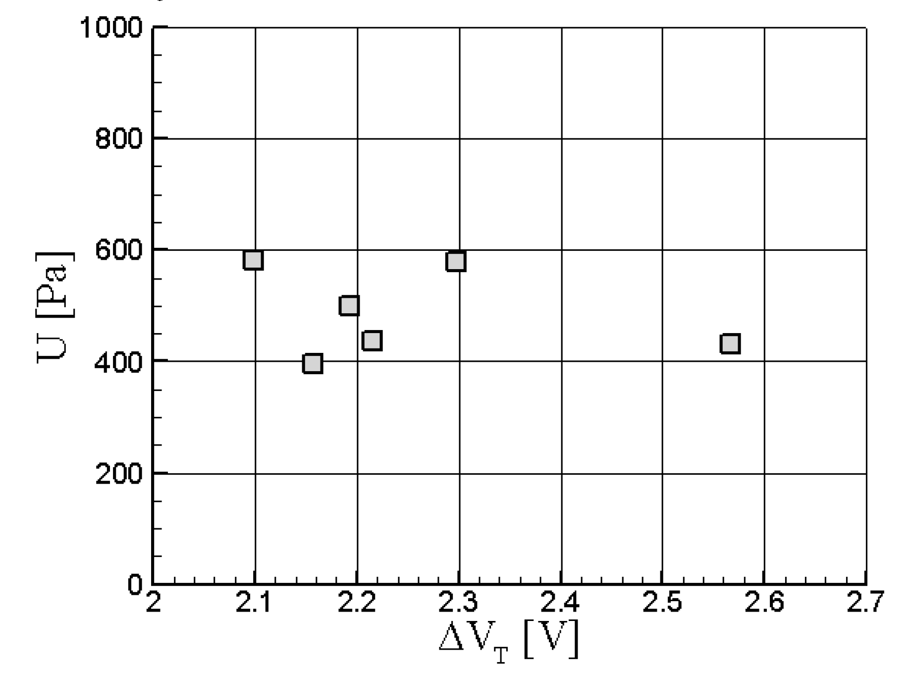
Uncertainty Quantification
The uncertainty evaluation was made by considering the uncertainty on each measured point in pressure for a given oven (probe) temperature and the contribution due to the least square interpolation among the pairs (Pi, ∆V
P,i). The contribution on the single measured point takes into account the standard deviation of the population, the reference transducer uncertainty, and the data acquisition board analog-digital converter specifications. Gaussian distribution was considered for the first two quantities while a rectangular distribution was applied to the AD converter. All these contributions are considered not cross correlated, are made homogeneous in terms of units, and are considered to include 95% of the Gaussian distribution data: finally, given the functional dependence f = f(x1, x2, …, xn), the uncertainty propagation approach is considered:
To couple the uncertainty on the single calibration point and the one due to the least square interpolation, the highest among the single points one is considered. Overall, for a 6-bara transducer, the following results were found (
Figure 5): no clear trends are visible and data less than 0.1% of the full range. These results are then applied during the aerodynamic calibration to get an estimation of the flow field detection uncertainty.
With the aim of comparing classical uncertainty analysis with an alternative systematic approach, the Montecarlo methodology was also applied and the same contributions to the uncertainty were considered. The data for each temperature level (Ti) were interpolated by a least square method by introducing N (a number high enough to get a statistical reliability) different pairs (P, ∆VP) chosen randomly into the populations characterized by the selected distributions. The results of the N calculations were N line constants and intercepts, statistically treated to obtain mean values (KPi, QPi) and their standard deviations. As a following step, M (a number high enough to get a statistical reliability) pairs of data belonging to the population (KPi, ∆VTi) were randomly chosen according to a Gaussian distribution, then averaged to get KP = KP (∆VT) and its standard deviation; the same methodology was applied to the intercept. In this way, P = P (∆VP, ∆VT), and its standard deviation were available for the application in the aerodynamic calibration.
To get a proper accuracy, the Montecarlo procedure requires a huge number of iterations: to make the procedure affordable, the Latin hypercube methodology was applied to support pairs choice, and a convergence criterion was also set on the standard deviation value. The results received by the two methodologies show a good consistency and were the basis for the determination of the uncertainty in the aerodynamic calibration.
Figure 6 shows the results of the uncertainty calculation when reported on the same chart of the probe pressure for a Mach = 0.5 test: the average uncertainty covering 95% of the samples is about 5 mbar (less than 0.1% of the transducer range), that is the same order of magnitude as the previous methodology.
4. FRAPP Dynamic Analysis
The manufacturing concept of the FRAPP developed at PoliMi implies a promptness reduction with respect to that of the sensor installed within the probe due to the line-cavity system between the pressure tap and the sensor’s sensitive element. However, a proper design of the internal cavities allows to obtain a promptness of 80 kHz, as shown in [
23].
To achieve such a promptness, the probe transfer function has to be experimentally determined and then applied in the data processing of measurements in test-rigs. However, the use of the transfer function for experiments downstream of turbomachinery rotors poses specific problems due to the inherent complexity of dynamic calibration tests since the operative conditions are often different between calibration and tests. These aspects are discussed in detail in the following.
4.1. Time- and Frequency-Domain Identification
The dynamic calibration of fast-response pressure instrumentation poses, at first, technical issues related to the generation of input signals featuring unsteady perturbations at sufficiently high frequency. Siren disks [
30] are used to generate periodic stimulus signals while shock tubes [
6,
24], are used to generate a transient non-periodic signal, as the travelling shock wave produces a step signal in very good approximation.
Shock tubes are preferred as, in a single test, the dynamic response of the probe can be achieved for the full frequency range typically of interest for turbomachinery applications (100 kHz). Considering air at ambient conditions, the dynamic content of a traveling shock involves frequencies up to the order of MHz. By setting proper diaphragm features, shock amplitude can be selected in the range of typical pressure fluctuations in turbomachinery (in the order of tenths of bars or even less as authors documented in [
7,
8,
11,
12]; such perturbations are normally small enough to not activate relevant non-linear effects in the dynamic evolution of the pressure field within the line-cavity system. By virtue of such physical linearity, the transfer function determined through the step-response is applicable for the measurement of the periodic fluctuations occurring within turbomachinery.
Since the beginning of this research 20 years ago, continuous improvements have been made on the low-pressure shock tube presented in [
24], in particular on the bursting diaphragm; by using the present-day plastic materials, shock strengths of the order of 0.2–0.3 bars were obtained. They exhibited incomplete opening whose effects were investigated in detail in [
31]; such effects can be properly handled in order to minimize their impact on the determination of the probe transfer function.
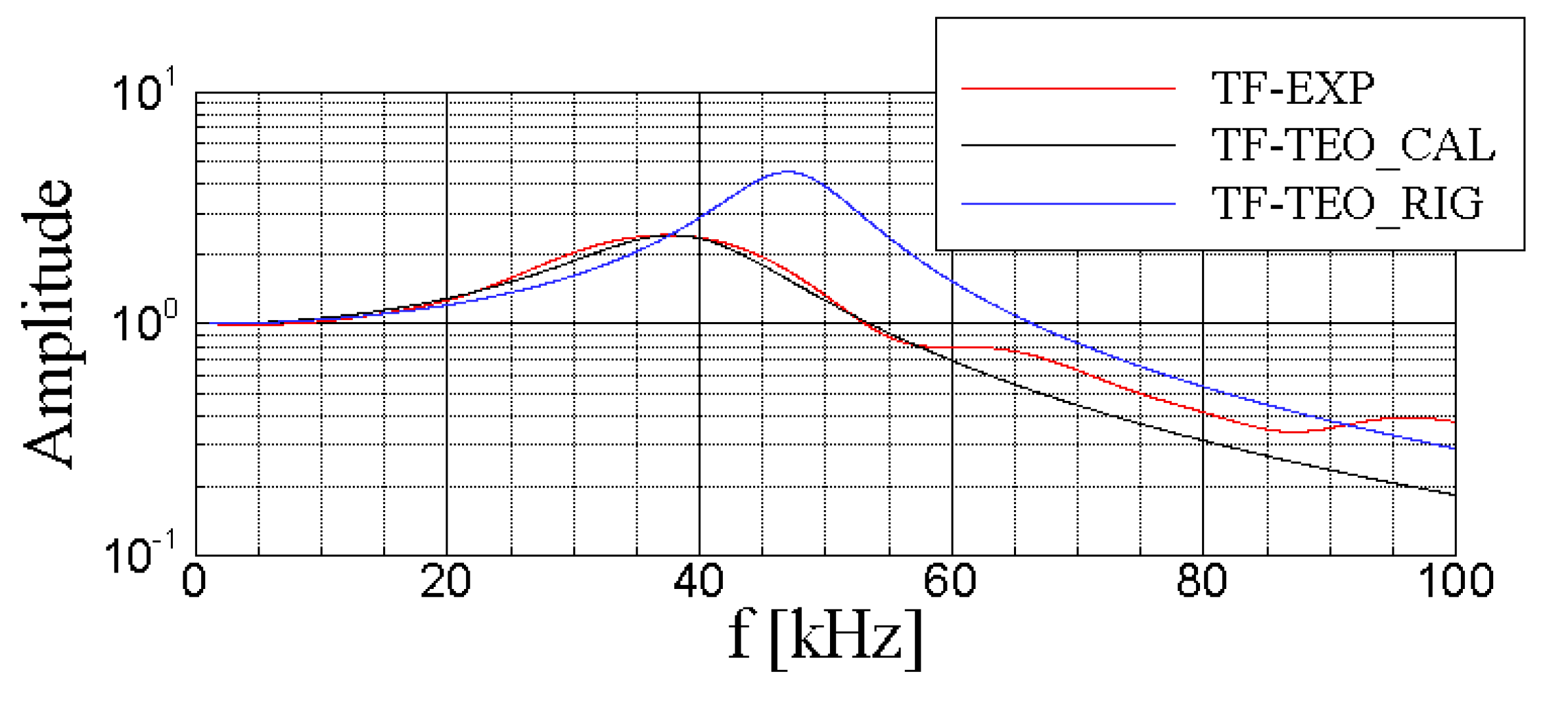
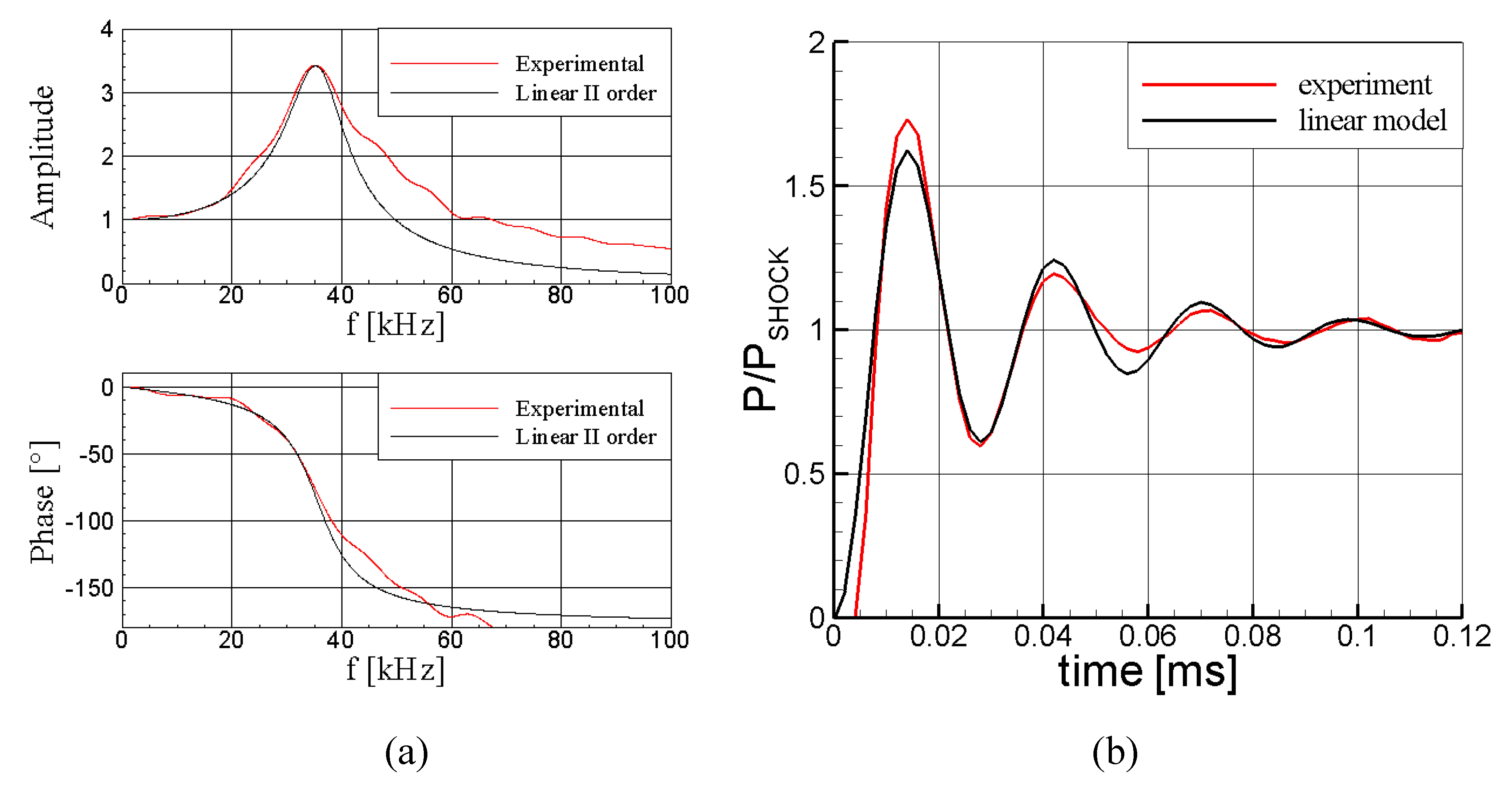
Figure 7a presents a typical experimental transfer function obtained with the method proposed in [
24]. The experimental trend recalls closely the one of a second-order linear system, with an evident peak at about 35 kHz representing the probe line-cavity system resonance. On the basis of the frequency and amplitude at resonance, the system identification can be done: the corresponding linear system is also plotted in comparison to the experimental one. Differences exist but occur at a high frequency (above 40 kHz). To provide a more intuitive idea of the observed non-linearity, the measured step response and the analytical response are plotted in
Figure 7b. The experimental trend reproduces well the one of the analytical model, suggesting that the modelling is reliable for the whole response. The largest difference is concentrated in the first overshoot in which the experiment exhibits a steeper pressure rise and a higher peak. The faster pressure rise at the beginning of the process is clearly responsible for the non-linearity observed in the frequency domain beyond 40 kHz. Since full linearity is not guaranteed a priori, experimental dynamic calibration is crucial to determine the transfer function of each FRAPP manufactured in order to properly compensate the measured signals.
4.2. Pressure and Temperature Correction
Thanks to the good linearity exhibited by the FRAPP, the use of the transfer function to dynamically compensate the pressure signals measured in turbomachinery test rigs is possible, at this stage. Notwithstanding that the thermodynamic conditions of the fluid in test rigs are often different from those occurring in the shock tube and considering that, in general, it is not possible toreproduce such conditions in the shock tube facility, relatively simple techniques can be proposed for correcting the transfer function identified in the dynamic calibration experiments. In [
23], the analytical model of [
32] was found to reproduce fairly well the resonance frequency of the FRAPP. This model, as well as the other ones available in literature, show that, apart from geometrical terms, the natural frequency and the non-dimensional damping of the line-cavity system exhibit the following dependencies:
Expression 4, which relates directly the natural frequency to the sound speed, is intuitively justified as the dynamic response of the line-cavity system depends on the pressure wave propagation within the probe internal cavities. In the context of perfect gases, this property provides a first straightforward correction to the transfer function for temperature differences between calibration and application. Expression 5 indicates that both temperature and pressure levels have an impact on the damping and, once again, it provides a tool for correcting the transfer function identified with experiments in the shock tube; also, the pressure level can have an effect and demands for corrections, even though its effect is quantitatively lower than that of the temperature.
Figure 8 shows the impact of combined temperature and pressure correction on the amplitude of the transfer function determined in the shock tube (TF-EXP). For this probe, a nearly perfect dynamic linearity is observed up to 60 kHz, with natural frequency at about 40 kHz, as shown by the comparison with the analytical second order transfer function (TF-TEO_CAL). By considering an application at the maximum temperature level technically available for the FRAPP (550 K), a correction to the analytical transfer function was applied to get the analytical transfer function in the real environment of the test rig (TF-TEO_RIG). The impact of the corrections is negligible up to 20 kHz, while a relevant deviation occurs for a frequency higher than 40 kHz.
An application at high pressure and high temperature (not reported extensively for confidentiality reasons) showed that the linearized temperature-pressure correction allowed properly compensating the pressure signals measured by the probe, thus recovering the typical power spectra of unsteady pressure measurements in high-speed flows.
5. FRAPP Aerodynamics
The aerodynamic calibration was performed on a convergent nozzle whose outlet section is 50 mm × 60 mm and typically allows for neglecting the blockage effects up to Mach = 0.95. Convergent –divergent nozzles are also available when supersonic calibrations are required. The Reynolds–Mach number effects decoupling can be also achieved by a nozzle inserted in a duct brought to a chocked condition by a downstream throat. The outlet pressure is usually set to be atmospheric and the Mach number is set by imposing the total pressure in the upstream reservoir.
When the aerodynamic calibration is of concern, different calibration coefficients can be taken into account. The advantages of different coefficient sets may arise from a pure aerodynamic behavior or from the uncertainty point of view.
5.1. Cylindrical FRAPP
For the 2D Frapp probe, the following is commonly applied:
where
PL = probe Left pressure reading,
PR = probe Right pressure reading,
PC = probe Central pressure reading,
PT = nozzle Total pressure, and P
S = nozzle Static pressure.
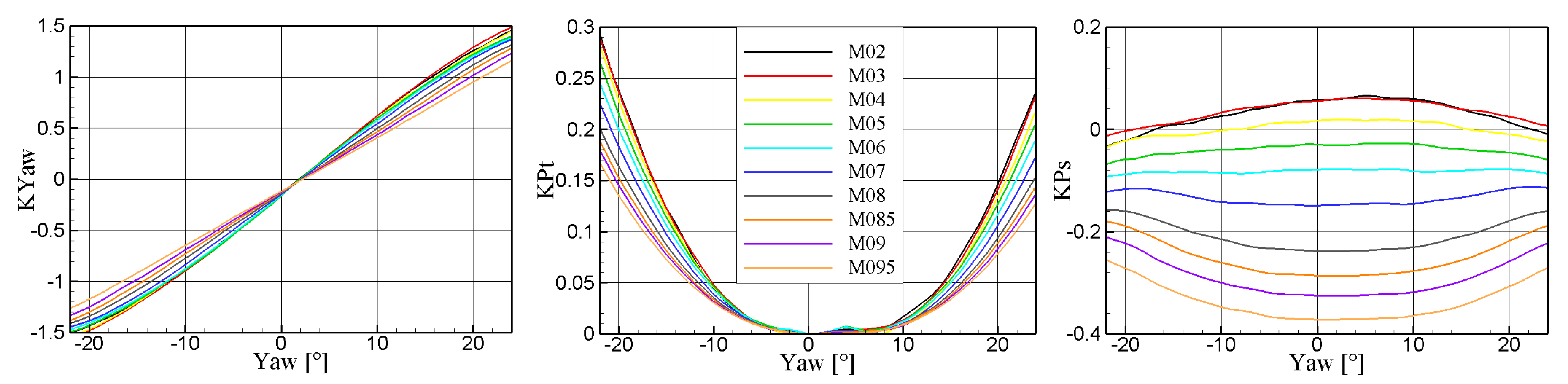
The experimental trends of the coefficients are reported in
Figure 9: when the Kyaw coefficient is zero, the aerodynamic reference direction is set. The range of monotonic trend is typically up to +/− 23°, due to the 45° of spacing between the three pressure readings (Left, Central, Right) and to the range in between the two flow separation points on a cylinder positioned in cross flow, that is around +/− 67° ÷ 70°. depending on the probe geometry, Reynolds and Mach numbers. The total pressure coefficient differs mainly for the compressibility effect over the probe cylindrical head, with the Reynolds number having a lower impact in this range.
In the application phase, the real Total and Static pressures (and by these the Mach number) and the flow angle are derived by an iterative procedure. First, the static pressure and the total pressure are chosen as the average between the left and right, and the central one, respectively; using these, the KYaw is a calculated and the yaw angle is derived. Using the yaw angle, the new KPt and KPs are calculated by making use of the calibration curves, properly interpolated in angles and Mach. At this point, the new Total and Static pressures are calculated and the second iteration can start.
In case of thermal drift, the KYaw is less sensitive than KPt and KPs because the numerator is almost insensitive to the drift, which typically occurs as an offset.
5.2. sFRAPP
For the 3D sFRAPP several sets of coefficients were considered and evaluated in calibration. Some of them are discussed separately in the following:
5.2.1. Set A
where
KYaw,
KPT and
KPS depend on the yaw tap (and its virtual readings) and on the flow total and static pressures, while the
KPitch depends on the Pitch tap (
PP) and on the flow total and static pressures. None of the coefficients are defined by mixing the pitch and the yaw taps and all include
PT and
Ps. The KPt is defined as usually found in the literature for multi-hole probes. KPs typically refer to the static pressure (
PS) and to the average of the lateral holes, whose value is close to the static pressure. In this probe, the lateral holes provide the pressure readings
PL,
PR, and
PP; however, these lateral holes are not symmetrical with respect to the probe head (as, instead, occurs for 5-hole probes of conical/prismatic head shape), and for this reason, the average of the corresponding pressure readings is always very different with respect to the actual static pressure of the flow, making the KPs coefficient not null in any condition. For this reason, only
PL and
PR are considered in the proposed KPs definition. As a further technical consideration, the
PP is measured with a different transducer with respect to
PL and
PR and thus, retaining
PP in the KPs definition would make the coefficient sensitive to the different potential thermal drift of the two transducers.
As for KYaw and KPitch, they have a definition consistent with multi-hole geometries, with KPitch being defined with only one tap (PT is a constant given the Mach number).
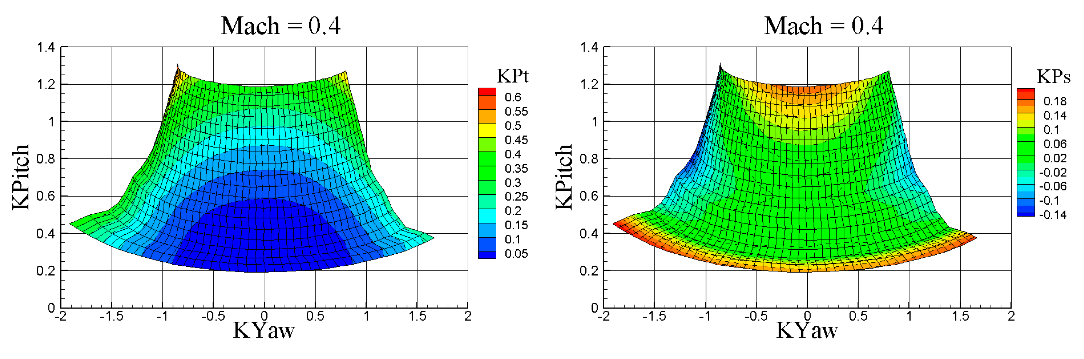
As reported in
Figure 10, the KPt and KPs coefficients are regular over the grid KYaw-KPitch and for this, they seem easily applicable. However, they exhibit an overlapping zone at the boundary of the matrix that leads to non-unique solutions during the interpolation procedure.
5.2.2. Set B
It differs from Set A only for:
, where
Pmax is the maximum value of the parabola passing by the three points
PC,
PL,
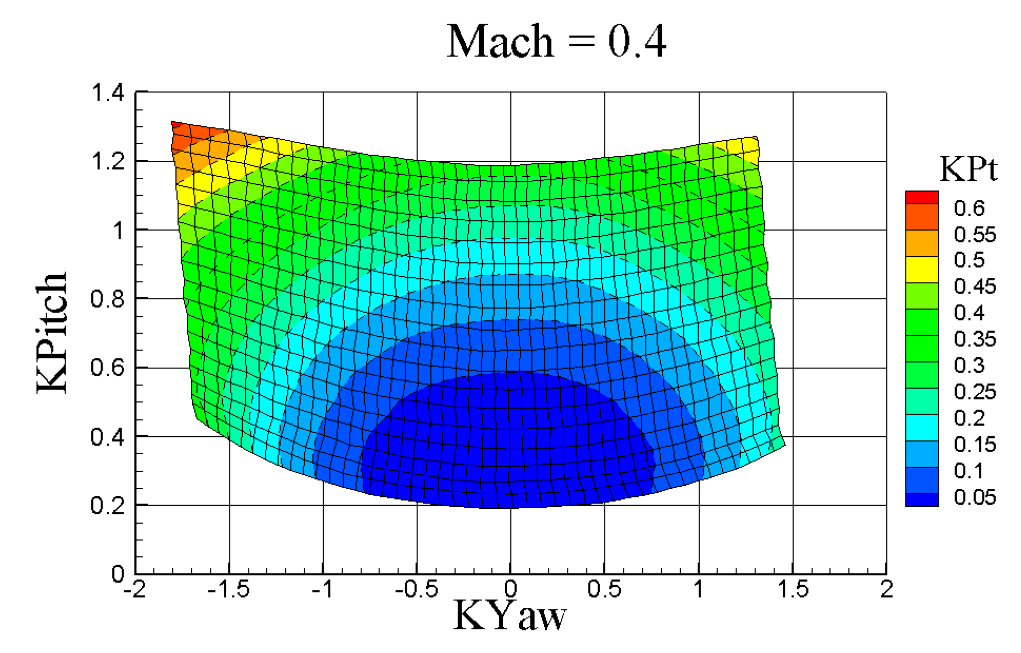
PR: it is an artificial value because the pressure curve around a cylinder is not a parabola, although it is similar to one. This new coefficient does not suffer from offset errors, being related to one transducer only and including differences both at numerator and denominator. A similar choice for the KPitch cannot be applied because there are no virtual taps for such a quantity as result of the rotation along the probe stem. The other main advantage concerns the grid regularity that allows for a proficient interpolation over the whole angular range, as visible in
Figure 11.
5.2.3. Set C
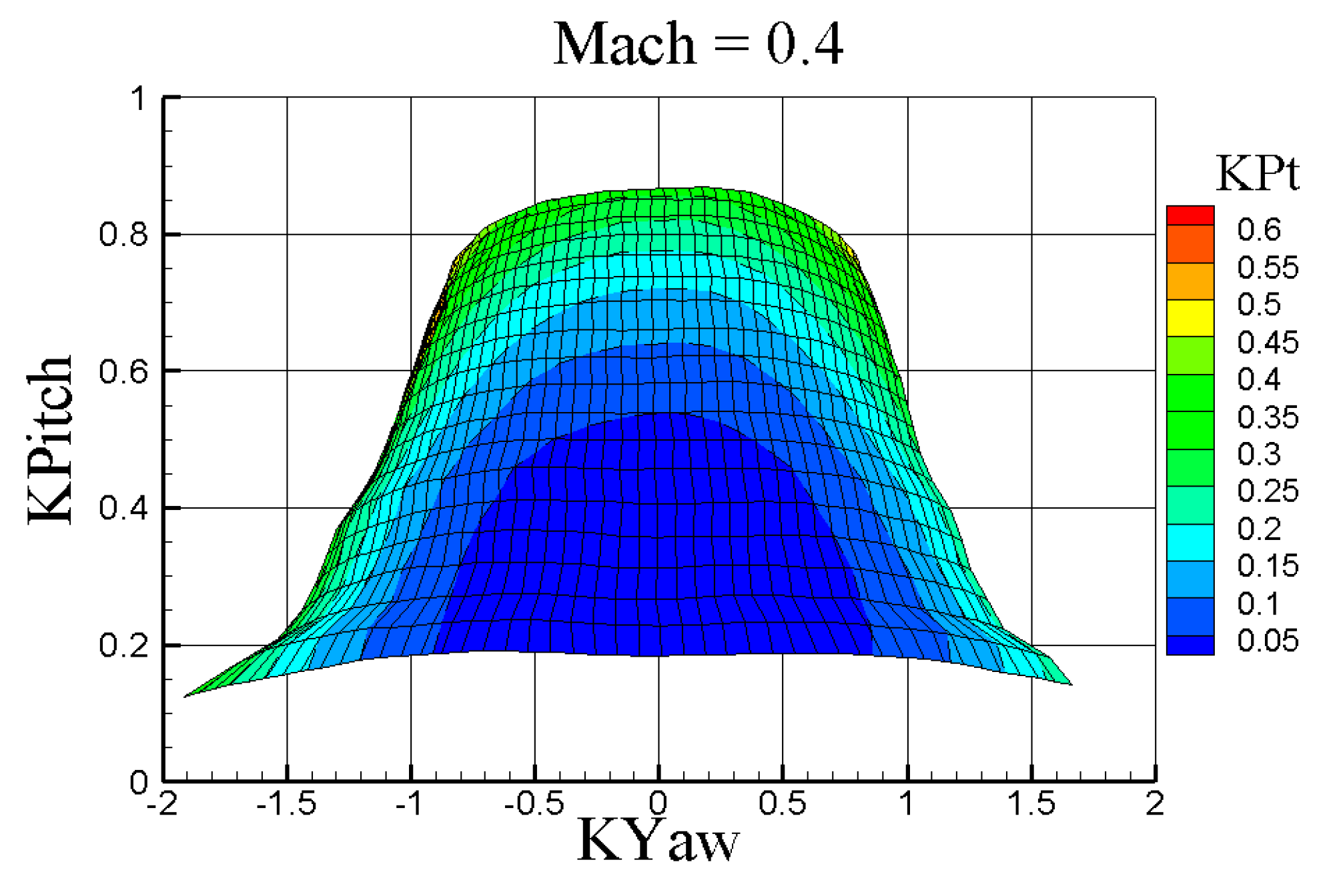
It differs from Set A only by the KPitch that is defined in this set as
. This choice allows for a direct link between the central reading of the yaw and the pitch tap, as the central reading for the yaw is, in any case, dependent on the pitch flow angle. This set, although seemingly smart, in fact, connects the two sensors readings and, in case of a thermal drift, it may increase substantially the final uncertainty. From a purely aerodynamic point of view, as shown in
Figure 12, it changes the KPitch coefficient magnitude but does not fix the overlap at the grid boundary.
5.2.4. Discussion on Coefficient Sets
Set A was abandoned because it does not guarantee a unique solution in the iterative procedure due to the overlap at the edges of the calibration matrices. Set C has the advantage of linking the pitch sensitivity to the most physical difference that is the (PC − PP): notwithstanding this fact, it was abandoned as well, due to the mixture of two transducers readings that make its application critical in the context of possible (and maybe difficult to compensate) thermal drift. Moreover, it does not allow to fix the problem of the non-unique solution at the edges of the matrices.
Set B was chosen for this type of probe as it provides both the advantage of keeping separate the two transducer readings and of the proper scaling of the angular sensitivity (
PL −
PR) to the local kinetic head measured by the probe, at that pitch position. To aid the physical understanding of this latter concept, i.e., of the artificial
Pmax,
Figure 13 reports the yaw tap pressure measurements (
PC) in the yaw calibration range for the different pitch angles. Two observations can be drawn:
- (a)
the maximum pressure depends on the pitch angle as a consequence of the tap position with respect to the flow direction: therefore, the Pmax allows for considering this difference.
- (b)
the difference between Pc at Yaw = 0° and Yaw =20° is slightly greater for negative pitches, where also (PL − PR) has higher values: the Set B denominator is then able to scale properly the angular sensitivity of the yaw tap.
5.3. Uncertainty Quantification
To quantify the uncertainty level in the calibration matrixes building and application, the same methodologies as those described in the static calibration can be applied. The results discussed in the following were obtained for the FRAPP probe. In this work, only uncertainties in the calibration and in the probe application when the probe was applied in a steady flow are considered: uncertainties due to probe installation and positioning, unsteady effects (e.g., the probe stem vortex shedding or possible interaction with the cascades), intrusiveness, and spatial discretisation are not considered as highly dependent on the kind of positioner used and on the application foreseen for the probe: in any case, besides the positioning, the other uncertainty sources are very difficult to be evaluated.
As the calibration matrixes require the application of iterative procedures, the Montecarlo methodology is particularly attractive for computing the uncertainty propagation.
The calibration coefficients (KYaw, KPt, KPs) were first calculated by choosing pressure values (PL, PC, PR, PT, PS) randomly in each population (for a given Mach number and angular position) according to the Gaussian distribution resulting from the static calibration (see the static calibration paragraph). Then, the results of the calibration coefficients were averaged and their standard deviation was calculated, then they were all stored in proper calibration files.
During the measurements campaign, to obtain the flow quantities, the measured pressures were used coupled to the calibration matrixes: the measured pressures were analysed by the same procedure applied in the calibration processes, leading to a gaussian distribution with their own mean value and standard deviation. A number N of different sets of pressures and coefficients were selected randomly in each population and by an iterative procedure, the flow quantities calculated. Since the process is statistical, all the data were then averaged and the standard deviation was calculated. As for the result distribution, since the input data were chosen according to a Gaussian distribution, the output ones were of the same kind. The number N of different sets was dynamically chosen according to the convergence criterion chosen for the standard deviation change (Δσi+1,i/σi < 10−3). Moreover, in this case, the set choice was made by applying the Latin hypercube methodology in order to save computational time.
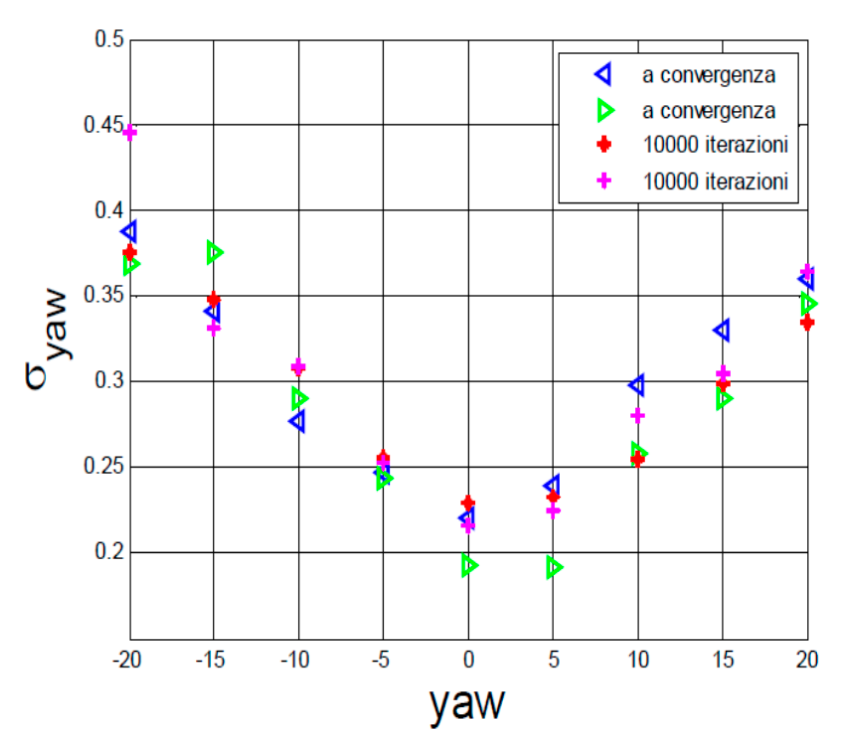
Figure 14 shows the results for different run and convergence criteria: since the method is based on statistics, different runs may lead to different results. Notwithstanding such possible variations, the difference is almost negligible for a given yaw angle. Finally,
Table 1 shows the averaged error for the four quantities of interest (Yaw, Mach, P
T, P
S). Values are high typically at low and high Mach numbers. At a low Mach number, this is due to the high transducer range that makes the transducer uncertainty quantitatively significant in the context of the measurements; at high Mach, the overspeed on the cylinder makes the flow locally supersonic and in this case, the measurements are less accurate.
6. Conclusions
This paper presented the most relevant developments in FRAPP technology at Politecnico di Milano in the last decade. This study considered the two most relevant probe configurations manufactured, calibrated and applied by the authors in their experience, for both 2D and 3D unsteady flow measurements in turbomachinery. Specific challenges emerged in terms of extension to (relatively) high temperature applications, simplicity of operation, improved aerodynamics and more refined uncertainty quantification, and were all acknowledged in the paper.
In particular, uncooled FRAPPs were manufactured for a temperature operation of about 550 K, without changing the external/internal probe shape and size. The need for high temperature extension also triggered specific theoretical models to handle temperature-corrected static and dynamic calibration of the probes. A physical analysis of the sensor properties and of the line-cavity system provided general rules for correcting the static and dynamic pressure measurements performed during calibrations. In the frame of these activities, the static and dynamic calibration procedures were re-analyzed to investigate the global reliability of the FRAPP technology.
The probe aerodynamics were also reconsidered and several sets of aerodynamic coefficients were proposed for the Spherical FRAPP, which is less consolidated with respect to the cylindrical one. This analysis highlights that clear advantages can be obtained if a specific set of coefficients is applied. Finally, a novel technique based on the Montecarlo approach was introduced to evaluate the uncertainty of FRAPP measurements, combining those of the sensor (based on a Montecarlo analysis of the static calibration) with the formulation of the aerodynamic coefficients.


