Article

Heat Transfer in a Square Ribbed Channel: Evaluation of Turbulent Heat Transfer Models †

1
Institute of Jet Propulsion and Turbomachinery, RWTH Aachen University, 52062 Aachen, Germany
2
MAN Energy Solutions SE, 46145 Oberhausen, Germany
*
Author to whom correspondence should be addressed.
This paper is an extended version of our paper in Proceedings of the 13th European Turbomachinery Conference on Fluid Dynamics & Thermodynamics ETC13, Lausanne, Switzerland, 8–12 April 2019; Paper No. 42.
Int. J. Turbomach. Propuls. Power 2019, 4(3), 18; https://doi.org/10.3390/ijtpp4030018
Submission received: 28 May 2019 / Revised: 3 July 2019 / Accepted: 8 July 2019 / Published: 12 July 2019

Abstract

:
This paper presents the results of integral heat transfer measurements taken in a square ribbed cooling channel configuration for evaluating heat transfer and turbulent flow characteristics in convective cooled gas turbine blades and draws a comparison with numerical results. The heated section of the channel is either smooth or equipped with 45 crossed ribs on two opposite walls. The first part of the paper describes the instrumentation and experimental setup in detail. The second part compares the numerical calculations with the experimentally determined results. The turbulent heat transfer is calculated using two common algebraic models and three implemented explicit algebraic models, each time in combination with an explicit algebraic Reynolds stress model. The numerical calculations show that the use of higher-order models for the turbulent heat flux provides a higher accuracy of the heat transfer prediction for both configurations. The best model is able to predict almost all results within the experimental uncertainties.

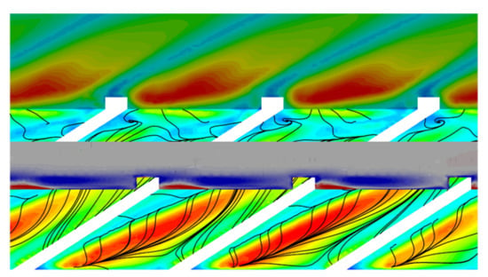
Graphical Abstract

1. Introduction

Even if the flow field in cooling channels is predicted correctly by numerical simulations, the prediction of the inner heat transfer still often deviates significantly from experimental data. Therefore, this paper focuses on new approaches for the closure of the Reynolds averaged energy conservation equation in simplified cooling channels.
The ERCOFTAC test case [1] was considered in the work carried out by Weihing et al. [2]. The turbulent heat transfer was determined with a constant turbulent Prandtl number and the explicit algebraic approach according to Younis et al. [3]. They were combined with several anisotropic Reynolds stress models [4,5,6,7]. A significant improvement in the prediction of the calculated Nusselt numbers could be achieved with a higher-order heat transfer model, with deviations of 10% compared to the experimental data. Rochhausen et al. [8] examined a backward-facing step. To close the Reynolds averaged conservation equation, the two-equation model k- ω according to Wilcox [9] was used. The averaged energy conservation equation is closed by a constant and variable turbulent Prandtl number [10] and a two-equation model [11], which solves transport equations for the temperature variance and its specific dissipation rate. The flow field was well represented, but no improvement of the heat transfer prediction could be seen by the use of the two-equation heat transfer model. This is because both models are based on the assumption of isotropic turbulence and thus the effect of anisotropy, which plays a significant role in the turbulent heat transfer, is not taken into account. Dietz et al. [12] investigated a backward-facing step measured by Vogel & Eaton [13]. Here, explicit algebraic heat transfer models [3,14] were compared to the approach of a constant turbulent Prandtl number in combination with the Reynolds stress model by Launder et al. [4]. The use of explicit algebraic models for the turbulent heat flux improved the prediction of heat transfer noticeably. This showed that it was possible to reduce the deviation with respect to the experiment from 25% to up to 8%. Dietz et al. [15] also investigated a delta-shaped vortex-generating element and compared the numerical results obtained using higher-order Reynolds stress and turbulent heat transfer models with experimental data. These investigations showed that the use of explicit algebraic models of the Reynolds stresses and of the turbulent heat flux [3] yielded the best results. The same conclusion was reached by Kobiela [16], whose investigations dealt with a rotating cyclone cooling chamber of a gas turbine blade. The heat transfer with a higher-order model for the turbulent heat flux by Younis et al. [3] deviated only by 10% from the experimental data, but by up to 30% with a constant turbulent Prandtl number.
This paper therefore deals with the potential of improving the prediction accuracy of the internal heat transfer in cooling channels. The study compares the numerical results of five different models for the turbulent heat flux, combined with an explicit algebraic Reynolds stress model, with experimental data in a smooth and a ribbed square channel. A more detailed discussion of the presented results can be found in Wörz [17].

2. Experimental Setup

The experimental data gained from the test rig based at RWTH Aachen University’s Institute of Jet Propulsion and Turbomachinery to analyse blade cooling configurations can be used to evaluate the numerical setup. The following section describes the test rig itself, as well as the two configurations investigated, including the heat transfer measurement technique.

2.1. Overview of the Test Rig

The test rig is used to make a detailed analysis of the flow field and to measure the integral heat transfer inside cooling channels section-by-section. Figure 1 gives an overview of the test rig with its measuring section, which consists of a square channel to enable the examination of the smooth and ribbed configuration. A second configuration, which represents a cooling channel geometry for a real convection cooled gas turbine blade, is planned for the future.
The air is provided in by a fan and then flows through a laminar flow element in which the flow rate is measured. To determine the Reynolds number, the mass flow is calculated from the flow rate and the density inside the air filter. The fluid then flows through an air heater, which heats the air to the desired temperature of 30 C. This ensures that the same temperature conditions prevail on different days in the measuring planes, which is necessary for the five-hole and hot-wire sensor measuring concept. The heater is connected to a nozzle for the transition to a square cross-section and to the adiabatic inlet section made of Plexiglas, which has a length of 26 hydraulic diameters d h . The hydraulic diameter is related to the square cross-section. A mixing grid for homogenizing the temperature is located behind the air heater. A turbulence grid located 6 d h in front of the heated measuring section sets the turbulence intensity at the inlet, depending on the chosen operating point. This can be applied as a boundary condition in the simulations. Before and after the 15 d h heated measuring section, the total and static temperature, as well as the total and static pressure, is measured at two fixed positions by means of a combined probe and static pressure holes. Both, the pneumatic and the hot-wire probes for measuring turbulent quantities, can also be traversed for further investigations.

2.2. Description of the Configurations

The configurations under investigation consist of a smooth and a ribbed square channel. The dimensions of the two configurations are identical and differ only on account of the copper segments, which are heated individually and used to determine the integral heat transfer coefficients. Figure 2 shows an overview of the ribbed channel configuration and the associated geometric parameters. Figure 3 represents the numerical domain, as well as the division of the plugs to determine heat transfer. The ribbed configuration uses 45 crossed ribs on two opposite walls. The other two walls are smooth which leads to a total of 23 pairs of ribs. This configuration was chosen because it had already been investigated in the literature [18] and it can therefore be compared with existing data, in addition to the supplementary measured values, to confirm the measurement concept.

2.3. Heat Transfer Measurements

Integral heat transfer measurements are carried out section-by-section on the test rig. For this purpose, each wall of the heated measuring section is divided into eight copper segments in flow direction. As some ribs would cross over adjacent copper segments, which might otherwise create a conductive path for heat to be transferred from one segment to another, ribs are milled into the copper as well as the isolation in between. All segments are adjusted to a constant wall temperature with the help of a heating foil attached to the outer wall of each segment. Since the copper segments have a very high thermal conductivity, the constant wall temperature can be determined by means of a single temperature measurement per segment. Due to specifying a uniform wall temperature (UWT), the thermal boundary layer has a continuous, uninterrupted profile. With a constant wall temperature, the heat flux on the copper segment and the bulk temperature, calculated by means of an energy balance, a heat transfer coefficient
α i = q ˙ W , i T W T bulk , i
per segment i is now formed. When comparing the numerical with the experimental data, it should be noted that the formulation of α i is carried out in exactly the same way. The expected errors are calculated by means of an error propagation according to Grabe [19], details can be found in Wieler [20]. They are between 5.8% and 11.4% for the Nusselt number as they increase with decreasing temperature potential between bulk and wall temperature. The difference between bulk and wall temperature is 30 K at the inlet of the heated section and 24 K respectively 18 K at the outlet for the smooth and ribbed configuration.

3. Numerical Setup

The numerical results presented in this paper are all calculated with ANSYS CFX 16.0. The following sections give an overview of the numerical setup for both configurations.

3.1. Modelling

For both configurations, the turbulent flow is modelled with the second order explicit algebraic Reynolds stress model (EARSM) of Wallin & Johannson [21]. The turbulent heat transfer occuring in the Reynolds averaged energy equation is calculated using five different models.
Two models are based on the gradient transport hypothesis, in which the turbulent Prandtl number is set to the constant value of 0.9 (Prt) or calculated as a function of specific flow variables (Prtvar) according to Kays [10], respectively. The turbulent Prandtl number is defined by
P r t = μ t c p λ t = turbulent momentum transport turbulent heat transport .
It represents a scaling factor between the turbulent viscosity and the turbulent heat flow. In this approach, no anisotropic effects are resolved, since P r t is a scalar quantity without directional dependency similar to μ t , what leads to an isotropic modelling approach. The turbulent heat flow in i direction
q ˙ t , i = ρ ¯ c i h ˜ = μ t P r t h x i
therefore depends only on the enthalpy gradient in this direction, other directions are neglected.
The remaining three models are explicit algebraic ones [3,14,22], which have been implemented by Wörz [17] in ANSYS CFX. These models calculate the turbulent heat flux in different ways, directly depending on the anisotropic Reynolds stresses. One of the first explicit algebraic approaches for the turbulent heat flux comes from Daly & Harlow [22]. Here, q ˙ t , i is directly related to the Reynolds stresses using a generalized gradient-diffusion approach
q ˙ t , i = c i h ˜ = C Θ 1 k ε c i c j ˜ h x j .
The turbulent kinetic energy k and the dissipation ε are known from the EARSM. C Θ 1 is a constant with a value of 0.3. The model presented by Abe & Suga [14] is an extension of the [22] approach, which simplifies the determination of the constant C Θ 2 used in this approach. Abe & Suga [14] introduced the Reynolds stresses normalized with respect to the turbulent kinetic energy k as a scaling factor, so that the turbulent heat flux
q ˙ t , i = c i h ˜ = C Θ 2 k ε c i c k ˜ c k c j ˜ k h x j .
Thus, the constant C Θ 2 is set to a value of 0.6. This value is recommended by Abe & Suga [14] for the far field. By analyzing the model using DNS data of a simple test case, Dietz et al. [12] showed that this value increases towards the wall, but not as much as the constant C Θ 1 in the Daly model. In the model of Younis et al. [3], there is a functional relationship between the turbulent heat flux and the other quantities, which occur in the transport equation of the turbulent heat flux. It is determined as follows
q ˙ t , i = c i h ˜ = C 1 k 2 ε h x i + C 2 k ε c i c j ˜ h x j + C 3 k 3 ε 2 c i x j h x j + C 4 k 2 ε 2 c i c k ˜ c j x k + c j c k ˜ c i x k h x j .
This is, therefore, the most comprehensive of the models used in this work. The gradient transport hypothesis (Equation (3)) and the Daly & Harlow approach (Equation (4)) can be found in the first two terms on the right. C 2 , C 3 and C 4 are constants that assume the values of 0.37, −0.0037 and −0.023. In the original formulation, C 1 was also a constant, but it is replaced so that the model can be used near the wall. The definition of this coefficient can be found in Wörz [17]. Due to the strong dependency on the Reynolds stresses, it is important to choose an anisotropic Reynolds stress model as a basis for the model variation.
In addition, the material properties of thermal conductivity λ , dynamic viscosity μ , and specific heat capacity c p of air are taken as temperature-dependent.

3.2. Meshing

All domains are meshed in an unstructured way with tetrahedra and prism layers in ANSYS ICEM CFD. This meshing strategy was chosen to bring about better transferability to more complex geometries in the cooling system of a real turbine blade. The deviations between a structured and unstructured mesh of representative parameters lie within the discretization error, which is specified later in this section.
All the models used need a high grid resolution in the region near the wall. Therefore, in both configurations 26 prism layers with an expansion ratio of 1.2 resolve this region, leading to the y 1 + values of the first grid node shown in Table 1. The dimensionless wall distance is defined as
y + = ρ y c τ μ with c τ = | τ W | ρ .
The discretization error is calculated using the approach taken by Roache [23]. This introduces the Grid Convergence Index (GCI), which estimates an infinitely fine mesh by means of a Richardson extrapolation from three different meshes. The mesh refinement is realized by doubling the resolution near the wall and by a coarser discretization of the far field area. The number of nodes of the selected meshes are 1.83 × 10 7 for the smooth and 2.02 × 10 7 for the ribbed configuration. Using these meshes, the discretization error of the smooth configuration is about 2.5% for the heat flux and 0.9% for the pressure loss. With respect to the ribbed configuration, the discretization error for the heat flux is 2.8% and for the pressure loss 0.1%. It can be seen that the influence of the discretization on the heat transfer is much more sensitive than on the flow field. All discretization errors are acceptable as they are in the order of magnitude of the expected experimental uncertainties.

3.3. Boundary Conditions

The boundary conditions of the fluid at the inlet correspond to a Reynolds number of about 65,000 based on the hydraulic diameter d h at an inlet temperature of 300 K. The turbulence grid upstream of the measuring section (shown in Figure 1) leads to a turbulence intensity of about 3% at the entrance of the heated section, which was measured with a triple-hot-wire probe. The turbulence intensity at the inlet of the numerical domain, which is 26 d h upstream of the ribbed domain, is therefore set to 5%, so that the same value as in the experimental setup is received. The corresponding integral turbulent length scale was calculated using the autocorrelation function, which was integrated up to the first zero crossing. The average value at the entrance is 4.8 mm for a Reynolds number of 65,000.

4. Results

In the following section, the investigation of the influence of different turbulent heat flux models in a square channel is presented. Two configurations are examined: one with four smooth walls and one with two ribbed and two smooth walls. To evaluate the different models, the numerical results are compared to experimental data from the test rig.
These simple geometries enable an investigation of the influence of a higher-order model of the turbulent heat transfer on the prediction accuracy of the results. The phenomena involved are sufficiently complex to show differences between simple and detailed modeling. From this, conclusions can be drawn about the necessity of such models in more complex, real geometries.

4.1. Smooth Configuration

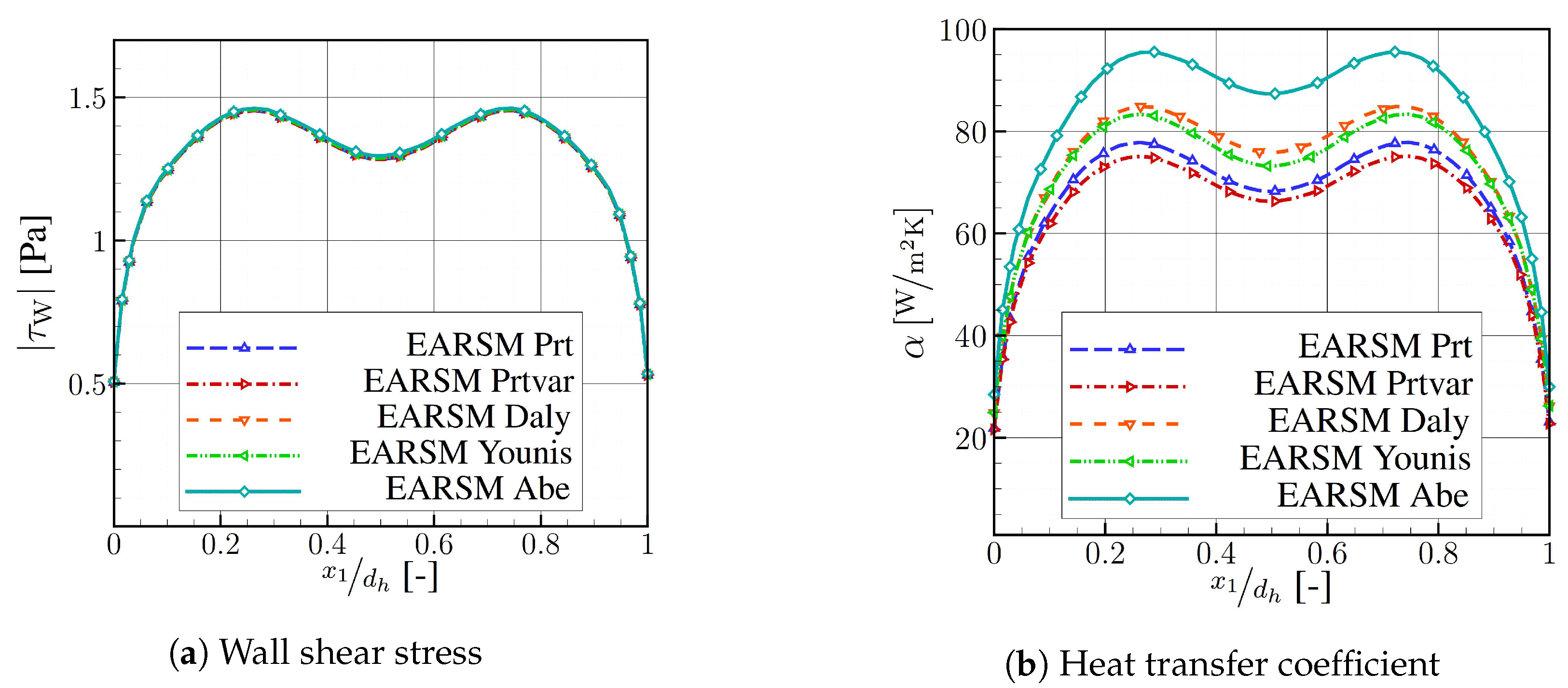
The different models for the turbulent heat flux have an influence only on the temperature field, not on the flow field. This is due to the fact that the very low Mach ( < < 0.3) and Grashof numbers in this particular case lead to a quasi incompressible flow and thus the two fields can be assumed to be decoupled. In order to confirm this, the wall shear stress τ W over the normalized channel width x 1 / d h is plotted in Figure 4a. On the right, the heat transfer coefficient α is shown for the five different models of the turbulent heat flux.
It can be seen that the wall shear stress is identical for all different heat transfer models. The heat transfer coefficient on the wall normal to the flow provides a different result. In the range 0.26 < x 1 / d h < 0.74, between the two global maximums, a parallel shift of α takes place. By using a variable Prandtl number, α is reduced by about 3% compared to a constant Prandtl number. This is because in this particular case the turbulent Prandtl number on the wall reaches a value of 1.7. And a higher turbulent Prandtl number leads to a lower heat transfer. The explicit algebraic models all provide an increase in the heat transfer on the wall. The model according to Abe should be mentioned here, as this provides an increase of up to 27% compared to Prt. The reason for the level shift, which results from the different explicitly algebraic models of the turbulent heat flux, can be explained by the constants selected in the respective approaches. The models for the turbulent heat flux according to Daly & Harlow [22] and Abe & Suga [14] in Equations (4) and (5) only differ in the value of the model constants and the extension in Abe for easier determination of this value. The constant chosen in the Daly model is 0.3, which is only half compared of the Abe model, and leads to a significantly smaller turbulent heat flux. The Younis et al. model [3] (Equation (6)) additionally includes three more terms, which are each provided with constants. However, since the second term in Equation (6), which occurs in all three models, is weighted more strongly in comparison to the other three terms with a constant of 0.37, it is conceivable that the turbulent heat flux calculated by the Younis model is only slightly higher than the one predicted by the Daly model.
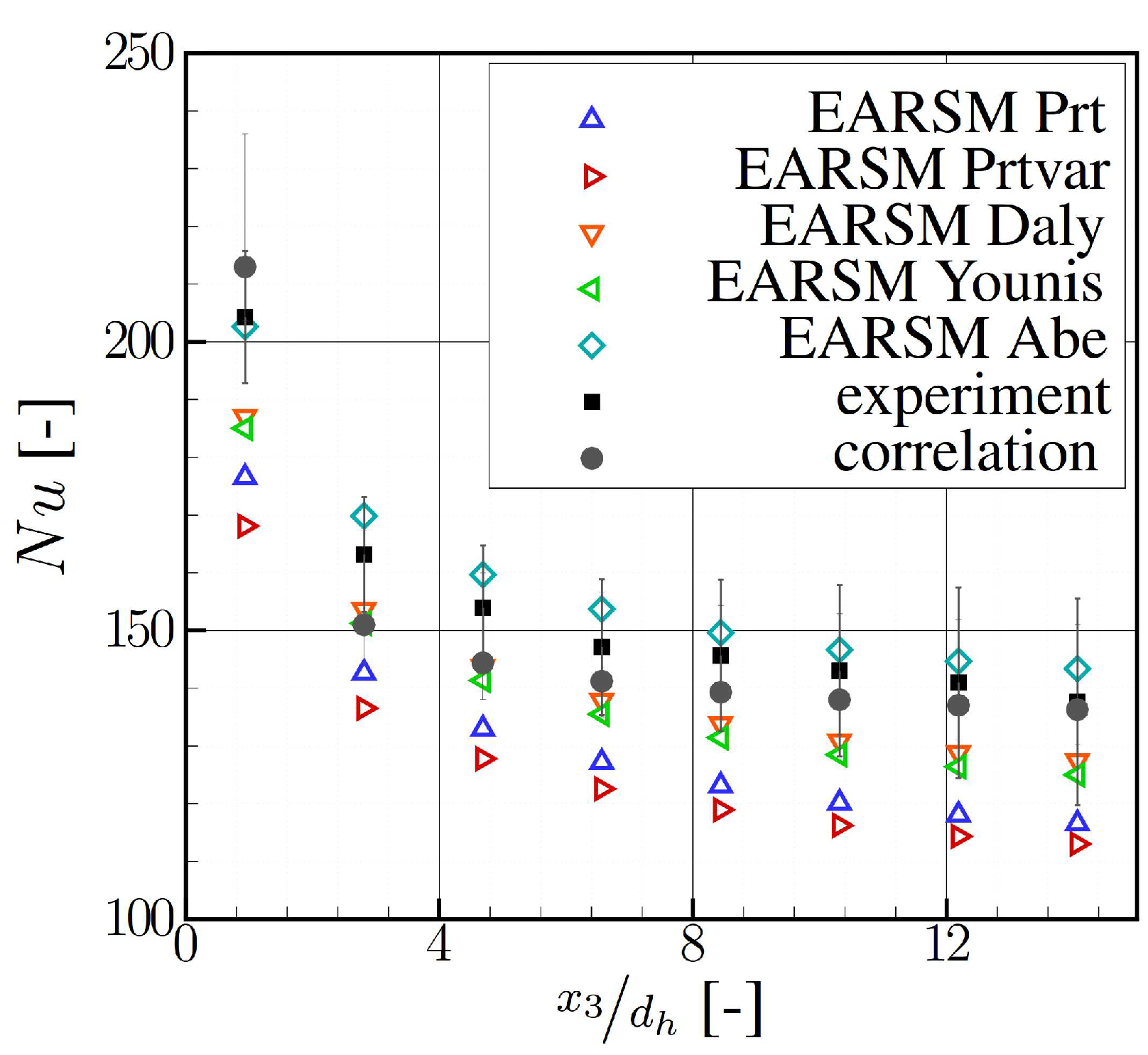
A comparison, using the average Nusselt numbers –measured section-by-section– is made to evaluate the different models. These Nusselt numbers, expressed by the heat transfer coefficient α i defined in Equation (1) are calculated for each copper segment and are shown in Figure 5. This comparison shows that only the Abe model is able to set the level of the Nusselt numbers to the level of the experimental data and therefore reproduce them satisfactorily. Using this model, all averaged Nusselt numbers that have been calculated are within the range of errors expected for the experimental data.
In addition, the semi-empirical correlation [24] for turbulent flow through a square channel is presented in Figure 5 in order to check the experimental determination of heat transfer. The calculation of the Nusselt number, depending on the Reynolds and Prandtl numbers, the pressure loss coefficient ξ , and the length x, reads as follows
N u x , t = ξ / 8 R e P r 1 + 12.7 ξ / 8 P r 2 / 3 1 1 + 1 3 d i x 2 / 3 with ξ = 1.8 log 10 R e 1.5 2 .
This semi-empirical correlation is valid for
10 4 R e = c i d h ρ μ 10 6 and 0.1 P r = μ c p λ 1000 .
All physical quantities in the dimensionless quantities included in Equation (8) are calculated on the basis of the arithmetic mean of the bulk temperature between inlet and outlet. The fact that the experimental data agrees with the semi-empirical approach therefore confirms the validity of the used measurement technology.
In summary, the standard model for turbulent heat flux (Prt) clearly underestimates the level of heat transfer in the smooth configuration. The results are only satisfactory when using higher-order models for the turbulent heat flux. For the best model combination for EARSM Abe, this results in the smallest deviation of predicted heat transfer compared to the experimental data.

4.2. Ribbed Configuration

The flow and the heat transfer in the ribbed channel are discussed briefly here in order to provide an overview of the present flow phenomena.
Figure 6 shows the heat transfer coefficient α calculated with variable bulk temperature on the ribbed and smooth wall of the second last copper segment, as well as the vorticity ω SW in the mean plane parallel to the main flow direction. At this position, the flow has already developed and barely changes in direction of flow. Directly behind the overflowed rib, there is a separation area ①, which develops into a vortex along the ribbed walls ⑤ close to the smooth wall. In this dead water area, the heat transfer is significantly reduced. Further downstream, between the ribs, is the dominant and large recirculation zone ②, which reattaches to the wall in the middle of the channel after about 65% of the rib spacing before the next rib ③. On the ribbed wall, the largest heat transfer occurs in the center of the recirculation zone ④, due to the strong mixing with the main flow. Depending on how the vortex of the recirculation area reattaches and how the vortex between the ribbed and the smooth wall ⑤ develops, this vortex hits the smooth wall more steeply or less steeply, leading to respectively higher or less high rates of heat transfer ⑥.
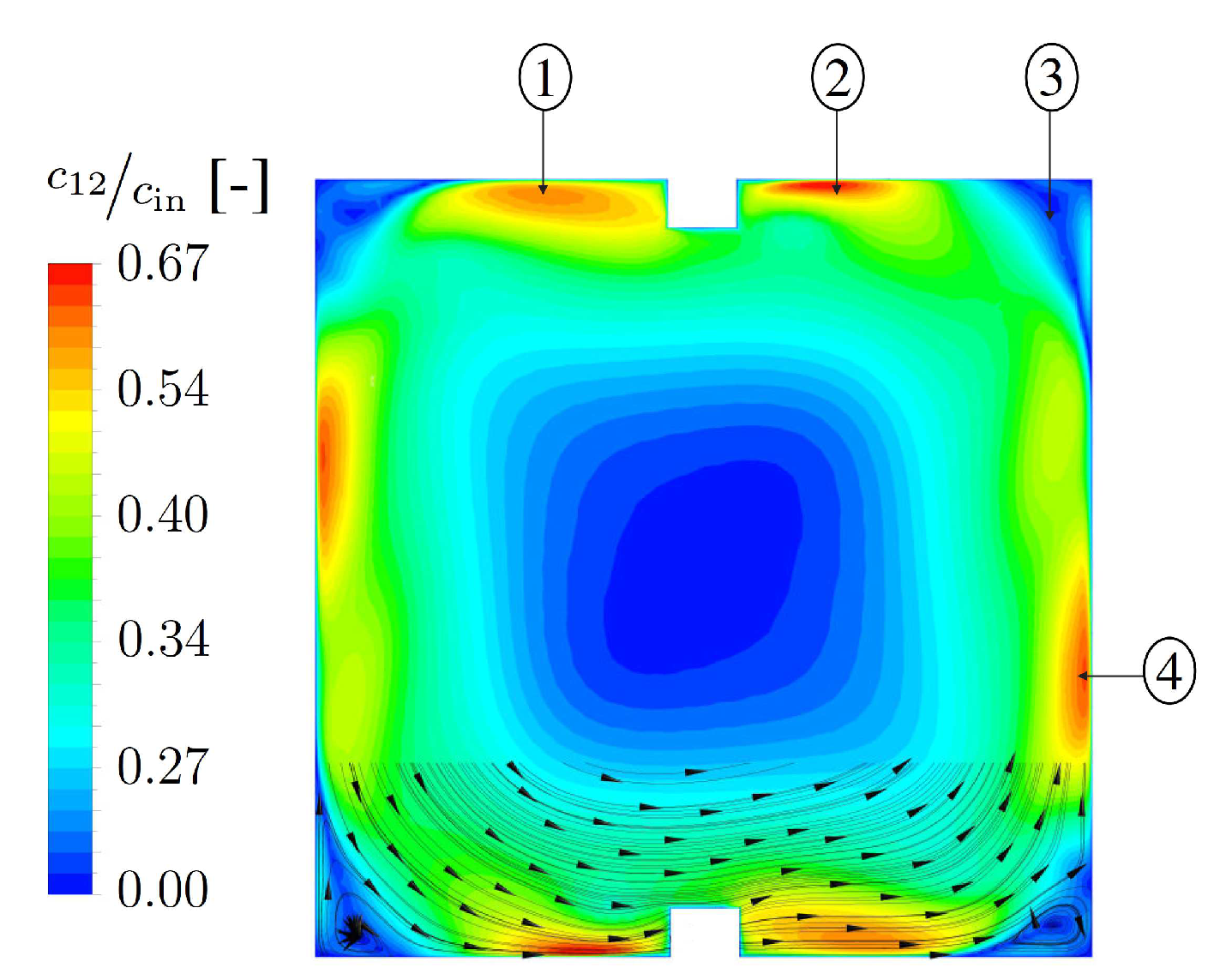
Figure 7 provides a better understanding of the secondary flows occurring in the ribbed channel. It shows the normalized secondary flow velocity c 12 in the direction of flow and some of the associated flow lines. With crossed ribs, a longitudinal vortex develops in the direction of flow, which is in the order of magnitude of the channel height. This vortex dominates the channel flow and leads to significantly improved mixing compared to smooth channels. The recirculation zones between the ribs, described in the previous illustration, can also be clearly seen in Figure 7. The area in front of and behind a rib can be seen at ① and ②, respectively. ③ is the vortex between the smooth and the ribbed wall, also mentioned above. The vortex of the recirculation zone of the previous rib has moved upwards along the smooth wall ④.
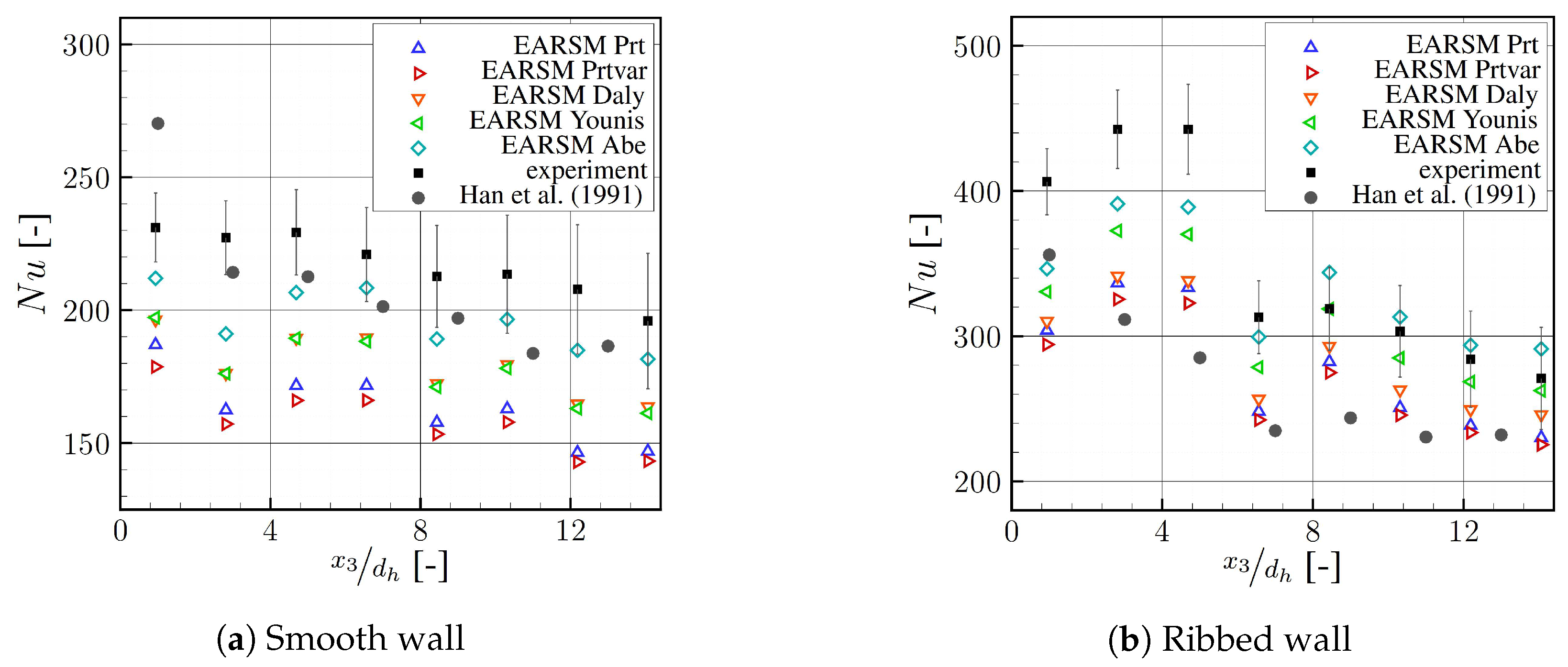
As with the smooth configuration, in the ribbed configuration, the anisotropic explicit algebraic Reynolds stress model is combined with the different models of the turbulent heat flux. Figure 8 shows the average Nusselt numbers calculated with the different models and the experimental data over the normalized channel length x 3 / d h for the smooth and ribbed heated copper segments. In addition, the experimental data of Han et al. [18] is presented in Figure 8. A direct comparison between the two experiments is difficult, as the boundary conditions are not similar and only the same geometric dimensions exist. In the experiment of Han et al. [18], a constant wall heat flux is applied to all copper segments, whereas in the experiment presented by Wieler [20] a constant wall temperature is selected to ensure an undisturbed boundary layer. Furthermore, Han et al. [18] uses brass ribs, which are glued onto the copper plugs. This leads to a different heat conduction within the solid compared to the plugs used by Wieler [20], which were milled completely out of copper.
In comparison with the experimental results of Wieler [20], the Abe model predicts the highest heat transfer and thus the heat transfer closest to the experimental data, as also seen in the smooth configuration. This is due to the choice of the constants selected in the individual models, as already explained in the previous section. On the smooth wall, the calculated values of EARSM Abe starting from the fourth copper segment are within the expected measurement error. However, the first three averaged Nusselt numbers are also underestimated by this model combination, with a maximum deviation of up to 15% in the second segment. Nevertheless, the higher-order modeling is a significant improvement compared to a deviation of about 30% for EARSM Prt in the same segment. This trend is also visible on the ribbed wall. From the fourth segment onwards, EARSM Abe and EARSM Younis lie within the measurement error and thus predict the level of the expected Nusselt numbers well. The decrease in the Nusselt numbers from the third to the fourth segment is underestimated and the increase from the fourth to the fifth segment is overestimated. This means that the Nusselt numbers for all models are underestimated in the entrance region of the channel. Starting from the fourth segment, the Nusselt numbers calculated are too high.
In summary the use of higher-order models for the turbulent heat flux leads to a significant improvement in the prediction accuracy of the heat transfer, without a noticeable increase in computational time. The increase of computational time with the combination EARSM Abe is less than 10% compared to the standard combination SST Prt09.

5. Conclusions

The investigations in this paper present the results of integral heat transfer measurements taken in two square ribbed cooling channel configurations for evaluating heat transfer and turbulent flow characteristics in convective cooled gas turbine blades and draw a comparison with numerical results. In both configurations (a smooth and a ribbed one), the use of higher-order turbulent heat flux models provide a significant improvement of heat transfer prediction. With regard to the smooth configuration, using the model developed by Abe & Suga [14] in combination with the EARSM of Wallin & Johannson [21], all averaged Nusselt numbers are within the expected measuring error. In the entrance region of the ribbed channel, this model combination underestimates the heat transfer by merely 15% at most compared to the experimental data, which is a major improvement compared to the 30% deviation with a constant turbulent Prandtl number. However, downstream of the fourth copper segment, all calculated Nusselt numbers are also within the expected measurement error. Therefore, it is recommended to model the turbulent heat flux with approaches of equal quality, in addition to higher-order modelling of the turbulent flow field.

Author Contributions

Conceptualization, B.W. and M.W.; Formal analysis, B.W.; Funding acquisition, M.R.; Investigation, B.W. and M.W.; Supervision, P.J.; Writing –original draft, B.W.; Writing –review & editing, M.W. and V.D.

Funding

The investigations were conducted as part of COOREFLEXturbo, a joint research program as part of AG Turbo. The work was supported by the Bundesministerium für Wirtschaft und Energie (BMWi) as per resolution of the German Federal Parliament under grant number 03ET7041A. The APC was funded by the Euroturbo Association.

Acknowledgments

The authors gratefully acknowledge AG Turbo and MAN Energy Solutions SE (Oberhausen) for their support and permission to publish this paper. The responsibility for the content lies solely with its authors.

Conflicts of Interest

The authors declare no conflict of interest.

Nomenclature

α heat transfer coefficient
q ˙ heat flux
Ttemperature
y + dim.less wall distance
d h hydraulic diameter
ρ density
ϵ turb. dissipation rate
μ dynamic viscosity
τ shear stress
N u Nusselt number
R e Reynolds number
P r Prandtl number
erib height
hspecific enthalpy
Cconstant
c p spec. heat capacity
at const. pressure
ω S W streamwise vorticity
c i velocity
x i coordinates
ξ pressure loss coeff.
Prib distance
kturb. kinetic energy
λ thermal conductivity
Hchannel height
at const. pressure

Sub-/Superscripts

tturbulent
fluctuation due to Favre averaging
Wwall
˜ Favre averaged
iindex
¯ Reynolds averaged

References

  1. ERCOFTAC. Two-Dimensional Flow and Heat Transfer over a Smooth Wall with Square Sectioned Ribs. Available online: http://sgk.me.umist.ac.uk/workshop/ (accessed on 2 February 2013).
  2. Weihing, P.; Younis, B.A.; Weigand, B. Heat transfer enhancement in a ribbed channel: Development of turbulence closures. Int. J. Heat Mass Transf. 2014, 76, 509–522. [Google Scholar] [CrossRef] [Green Version]
  3. Younis, B.A.; Weigand, B.; Spring, S. An Explicit Algebraic Model for Turbulent Heat Transfer in Wall-Bounded Flow With Streamline Curvature. J. Heat Transf. 2007, 129, 425–433. [Google Scholar] [CrossRef]
  4. Launder, B.E.; Reece, G.J.; Rodi, W. Progress in the development of a Reynolds-stress turbulence closure. J. Fluid Mech. 1975, 68, 537–566. [Google Scholar] [CrossRef] [Green Version]
  5. Gibson, M.M.; Launder, B.E. Ground effects on pressure fluctuations in the atmospheric boundary layer. J. Fluid Mech. 1978, 86, 491–511. [Google Scholar] [CrossRef]
  6. Speziale, C.G.; Sarkar, S.; Gatski, T.B. Modelling the pressure-strain correlation of turbulence: an invariant dynamical systems approach. J. Fluid Mech. 1991, 227, 245–272. [Google Scholar] [CrossRef]
  7. Dafalias, Y.F.; Younis, B.A. Objective Model for the Fluctuating Pressure-Strain-Rate Correlations. J. Eng. Mech. 2009, 135, 1006–1014. [Google Scholar] [CrossRef]
  8. Rochhausen, S.; Krüppel, F.; Fiedler, J. Numerical Treatment of Turbulent Low-Mach-Flow for Turbine Cooling Applications. In Proceedings of the 11th World Congress on Computational Mechanics, Barcelona, Spain, 20–25 July 2014. [Google Scholar]
  9. Wilcox, D.C. Turbulence Modeling for CFD; DCW Industries, Inc.: Flintridge, CA, USA, 1993. [Google Scholar]
  10. Kays, W.M. Turbulent Prandtl Number—Where are we? ASME J. Heat Transf. 1994, 116, 195–284. [Google Scholar] [CrossRef]
  11. Nagano, Y.; Kim, C. A Two-Equation Model for Heat Transport in Wall Turbulent Shear Flows. J. Heat Transf. 1988, 110, 583–589. [Google Scholar] [CrossRef]
  12. Dietz, C.; Neumann, S.; Weigand, B. A comparative Study of the performance of explicit algebraic models for the turbulent heat flux. Numer. Heat Transf. 2007, 52(Part A), 101–126. [Google Scholar] [CrossRef]
  13. Vogel, J.C.; Eaton, J.K. Combined Heat Transfer and Fluid Dynamic Measurements Downstream of a Backward-Facing Step. J. Heat Transf. 1985, 107, 922–929. [Google Scholar] [CrossRef]
  14. Abe, K.; Suga, K. Towards the developement of a Reynolds-averaged algebraic turbulent scalar-flux model. Int. J. Heat Fluid Flow 2001, 22, 19–29. [Google Scholar] [CrossRef]
  15. Dietz, C. Computation of Heat Transfer in Internal Flows with Vortex-Generating Elements. Ph.D Thesis, Universität Stuttgart, Stuttgart, Germany, 2008. [Google Scholar]
  16. Kobiela, B. Wärmeübertragung in Einer Zyklonkühlkammer Einer Gastrubinenschaufel. Ph.D Thesis, Universität Stuttgart, Stuttgart, Germany, 2013. [Google Scholar]
  17. Wörz, B. Numerische Modellierung Turbulenter Strömung mit Wärmeübergang in Einer Konvektiv Gekühlten Turbinenschaufel. Ph.D Thesis, RWTH Aachen, Aachen, Germany, 2018. [Google Scholar]
  18. Han, J.C.; Zhang, Y.M.; Lee, C.P. Augmented Heat Transfer in Square Channels with Parallel, Crossed, and V-Shaped Angled Ribs. J. Heat Transf. 1991, 113, 590–596. [Google Scholar] [CrossRef]
  19. Grabe, M. Grundriss der Generalisierten Gauß’schen Fehlerrechnung; Springer: Berlin, Germany, 2011. [Google Scholar]
  20. Wieler, M. Experimentelle Untersuchung von Strömung und Wärmeübergang Konvektiver Kühlsysteme in Turbinenschaufeln. Ph.D Thesis, Universität Stuttgart, Stuttgart, Germany, 2007. [Google Scholar]
  21. Wallin, S.; Johannson, A.V. An explicit Algebraic Reynolds Stress Model for Incompressible and Compressible Turbulent Flows. J. Fluid Mech. 2000, 43, 89–132. [Google Scholar] [CrossRef]
  22. Daly, B.J.; Harlow, F.H. Transport Equations in Turbulence. Phys. Fluids 1970, 13, 2634–2649. [Google Scholar] [CrossRef]
  23. Roache, P.J. Quantivication of uncertainty in computational fluid dynamics. Ann. Rev. Fluid Mech. 1997, 29, 123–160. [Google Scholar] [CrossRef]
  24. Gnielinski, V. Ein neues Berechnungsverfahren für die Wärmeübertragung im Übergangsbereich zwischen laminarer und turbulenter Rohrströmung. Forsch. Ing. 1995, 61, 240–248. [Google Scholar] [CrossRef]
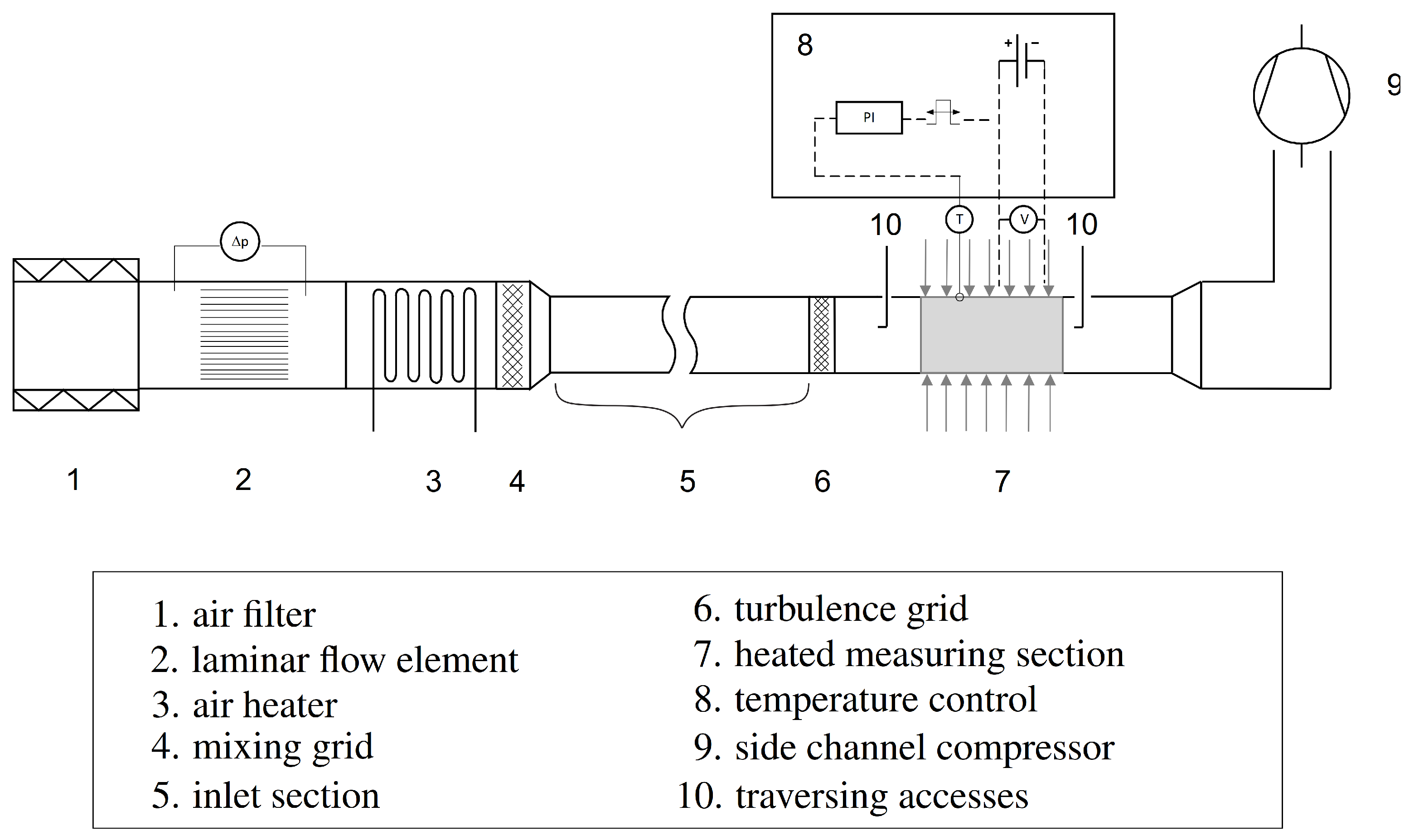
Figure 1. Overview of thecooling channel test rig.
Ijtpp 04 00018 g001
Figure 2. Parameter and overview of ribbed configuration.
Ijtpp 04 00018 g002
Figure 3. Overview of ribbed configuration and plugs.
Ijtpp 04 00018 g003
Figure 4. Values over normalized channel width along the wall at x 3 = 14 d h .
Ijtpp 04 00018 g004
Figure 5. Nusselt numbers over normalized length, experimental data, different models of turbulent heat flux, semi-empirical correlation [24].
Ijtpp 04 00018 g005
Figure 6. Heat transfer coefficient, vorticity parallel to main flow direction at 7-th plug.
Ijtpp 04 00018 g006
Figure 7. Normalized secondary flow velocity at x 3 / d h = 14 , view in flow direction.
Ijtpp 04 00018 g007
Figure 8. Averaged Nusselt numbers over normalized length, experimental data, different turbulent heat flux models.
Ijtpp 04 00018 g008
Table 1. Averaged and maximum y 1 + .
SmoothRibbed
smoothribbed
wallwall
y 1 , max + 0.090.350.18  
y 1 + ¯ 0.0750.10.1