1. Introduction
Due to the limited space for new establishments, there are more and more wind turbines placed in cold climate areas. These areas also have the advantage that the colder air has higher density, and because of this, there is the possibility to harvest more energy for the same wind speed.
The major impediment for wind turbines in cold climate is ice accretion which adds extra weight to the turbine components, imbalances the rotor and decreases the aerodynamic efficiency of the blades. A thorough review of cold-climate related issues is presented in the report of Laakso et al. [
1].
Besides the above-mentioned engineering challenges, ice accretion leads to safety issues as well: ice chunks might detach from the turbine components (most commonly from the blades) and fly to considerable distances, presenting a safety hazard for the persons or objects in the vicinity of the turbine. Even if the turbines are most often stopped when ice accretion occurs (to avoid damages), ice throw can still be a considerable risk, partly because ice chunks might detach already before the ice detection system stops the turbine, and partly because of the ever increasing height of the turbines, the ice chunks might travel long distances even if the turbine is parked.
Since in many cases the public might have access to the areas where wind turbines are located, it is important to accurately estimate the risks due to ice throw. In the vicinity of highly frequented places (ski resorts, public trails or roads), the safe distance to the wind turbine is an extra factor which needs to be accounted for in the already difficult process of finding optimal locations for new turbines. Le Blanc et al. [
2] report example risk assessment calculations for such cases.
Experimental investigations of ice throw are rather difficult. Most works consist of on-site observations, which have the drawback that they are done (due to the above-mentioned risks) a-posteriori. This means that there is no information about the release locations of the ice pieces and their initial size, since they may break during the flight or upon impact. Furthermore, melting between the time of impact and time of observation might also alter the size. Nevertheless, on-site observations lead to important estimates of the impact locations. Within the Alpine test site Gütsch project [
3], ice chunks with a maximum weight of 1.8 kg were observed in the vicinity of a 50 m hub-height, 40 m rotor diameter wind turbine. The maximum observed throwing distance was 92 m. Seifert [
4] summarises both previous results from the Wind Energy Production in Cold Climate (WECO) [
5] project and own data. The formula used as common practice to determine the safety distance
d, around a wind turbine in terms of the hub height
H, and rotor diameter
D, is also given in [
4] (Equation (
1)).
Besides on-site observations, most risk estimates are numerical evaluations of the ice trajectories. One of the early estimates of ice trajectories is reported in [
6] where the ice pieces are assumed to be point-like objects travelling under the action of gravity and aerodynamic drag force. The lift force is neglected based on the argument that the object is expected to tumble during the flight and the effect of the lift force is expected to cancel approximately. In [
7] the risk factors associated with wind turbines located in the vicinity of highways are estimated. Besides parts originating from a failure of the wind turbine itself, the case of ice throw is evaluated as well. The trajectories of the ice chunks are calculated by assuming a constant drag coefficient of 0.6.
In the recent work of Biswas et al. [
8], besides a thorough sensitivity study of the ice trajectories carried out with the traditional method, the influence of lift force is assessed as well. For this purpose the trajectories of plate-like objects, assumed to have angle of attacks for high lift, were tracked. The trajectory computations revealed that the lift force might indeed significantly change the trajectories, and by this the impact locations.
Here we also present numerical estimates of the ice trajectories. In the first part, three-degree-of-freedom (3DOF) calculations are used to carry out a sensitivity study of the impact locations to the ice release position, wind velocity, turbine rotation and aerodynamic drag coefficient. In the second part, six-degree-of-freedom (6DOF) computations are carried out to assess the importance of the aerodynamic forces normal to the ice trajectories as well as the importance of the object rotation.
2. Method
Since three-dimensional (3D) computational fluid dynamics (CFD) computations of the two-way interaction between the air and the flying ice chunk would be computationally too exhaustive, practical trajectory computations are based on one-way interaction, i.e., the ice chunk does not affect the wind velocity field. Therefore, this practical approach is adopted herein. As a result, the ice chunks are tracked as point-like objects subject to gravity and aerodynamic forces. The wind velocity field is assumed to obey a logarithmic law given by Equation (
2), the von Kármán constant being assumed to have the value
and the values of the friction velocity (
) and surface roughness height (
) are listed in
Table 1. The values are chosen to match the set-up reported in [
8]. The only exception is the sensitivity study to the wind velocity magnitude, where a flat wind velocity profile was assumed in the comparison.
In the 3DOF computations, the ice trajectory is governed by Equation (
3) which is integrated for the time being with a first order Euler method, but with adaptive timestepping where the timestep is adjusted to assure that the ice chunks will not travel a longer distance than a given threshold during a timestep. Comparisons with fourth order Runge-Kutta simulations [
8] (see
Section 3.1.1) reveal that the current method has sufficient accuracy.
For 6DOF computations, the dynamic equation for rotation (Equation (
4)) needs to be resolved as well. In Equations (
3) and (
4), it is assumed that the origin of the body-fitted coordinate system is at the center of gravity.
A complicating issue related to the tracking of rotating objects in 3D is the representation of the object’s attitude relative to the world coordinate system. Euler angles are commonly used, for example, in flight dynamics, however, they are prone to singularities for certain object orientations. This issue can be handled by tracking at least two sets of Euler angles, however, this complicates the implementation. Rotation matrices do not suffer from the problem of singularities, however, they have larger storage requirements and are relatively difficult to handle. Herein, quaternions are used to track the attitude of the objects, since they are not prone to singularities, have low storage requirement (only four components) and can be combined similarly to rotation matrices to impose complex rotations.
Force and Momentum Coefficients Database
Two-dimensional aerodynamic computations are commonly carried out based on databases of the drag and lift coefficients for several angles-of-attack. In 3D, the situation is more complicated, since there is no single angle which can describe the orientation of the relative velocity. In the present article we use the versors of the relative velocity to identify individual cases.
To populate the database, CFD computations are carried out to compute the aerodynamic forces and moments acting on the ice chunk for several different directions of the relative velocity. The magnitude of the forces and moments are normalised by the velocity magnitude square and the square (for the forces) or cube (for the moments) of a lengthscale specific to the object. The dependence on the Reynolds number could be added in future studies as an extra dimension in the database.
During the trajectory computations, the required force and momentum coefficients need to be interpolated depending on the instantaneous orientation of the relative velocity in the body-fitted coordinate system.
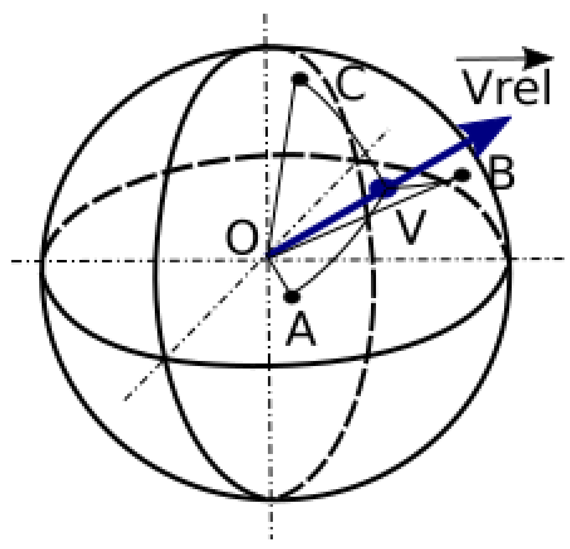
Figure 1 visualises the procedure. In
Figure 1, the points labelled A, B, C denote positions on the unit sphere for which data exists in the database, the blue arrow indicates the direction of the relative velocity for which the force and momentum coefficients are needed and V is the point where this relative velocity vector intersects the unit sphere, i.e., the position where we need to interpolate the data. The interpolation is carried out proportionally to the inverse distance along the unit sphere surface to the two closest known points, i.e., if A and B are the closest points,
,
being the force or momentum coefficient to be determined and
is the length of the arc on the unit sphere between points
X and
V, computed as
.
3. Results
Two sets of results have been computed. First, the trajectories of ice chunks are computed taking into account only the translation of the ice chunks. Since, to our knowledge, no available experimental data exists, the set-up matches the conditions reported in [
8] and the results are compared to the results therein. The main goal of this section is, besides validation, to assess the influence of azimuthal and radial release position, wind velocity and the drag coefficient of the ice chunk on the impact positions.
The second set of results targets the trajectories of ice chunks with 6DOF motion. The main objective of these results were to assess differences compared to point-like objects for parked and rotating wind turbines. Furthermore, the sensitivity to the quality of the force and momentum coefficient database has been investigated as well.
3.1. Trajectories Neglecting Rotation
In order to verify the implemented method, the case reported by [
8] has been set-up. The wind velocity is approximated by a logarithmic profile (see Equation (
2)). The main parameters of the set-up are summarised in
Table 1. The wind is blowing in the positive
z direction, gravity points in the negative
x direction. For initial conditions it is considered that the initial velocity of the ice chunk matches the blade velocity at the release position. The logarithmic profile has a hub-height wind speed of approximately 15 m/s.
Table 1.
Summary of the case set-up for 3DOF object trajectories.
Table 1.
Summary of the case set-up for 3DOF object trajectories.
| Parameter | Symbol | Value |
|---|
| Tower height | H | 100 m |
| Blade radius | R | 45 m |
| Rotor speed | | 14.5 rpm |
| Friction velocity | | 0.6514 m/s |
| Surface roughness | | 0.01 m |
| Ice mass | m | 1 kg |
| Ice frontal area | A | 0.01 m |
| Ice drag coefficient | | 1.0 |
3.1.1. Influence of Azimuthal and Radial Release Positions
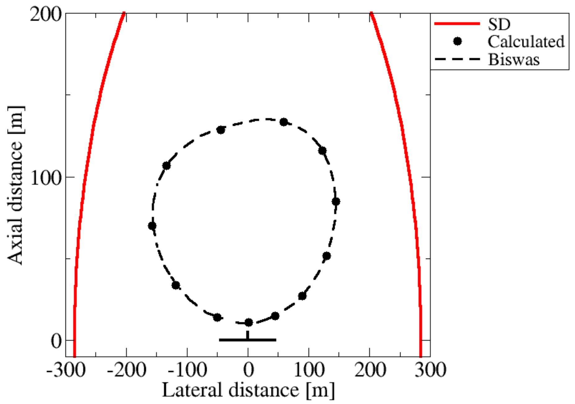
Figure 2 shows the computed impact locations for ice chunks released at the blade tip for varying azimuthal release angles. The axes are scaled differently in the figure to improve readability. The filled circles show the positions computed with the implemented algorithm; the dashed line shows the results reported in [
8]. As one can observe, the results match very well. The continuous red line in the figure (marked with SD in the legend) shows the location of the safety distance determined by Equation (
1). One can see that the impact positions are well within the safety zone. One can notice also the asymmetric shape of the impact pattern, due to the fact that the release velocity has the opposing sign on the vertical component on the two sides.
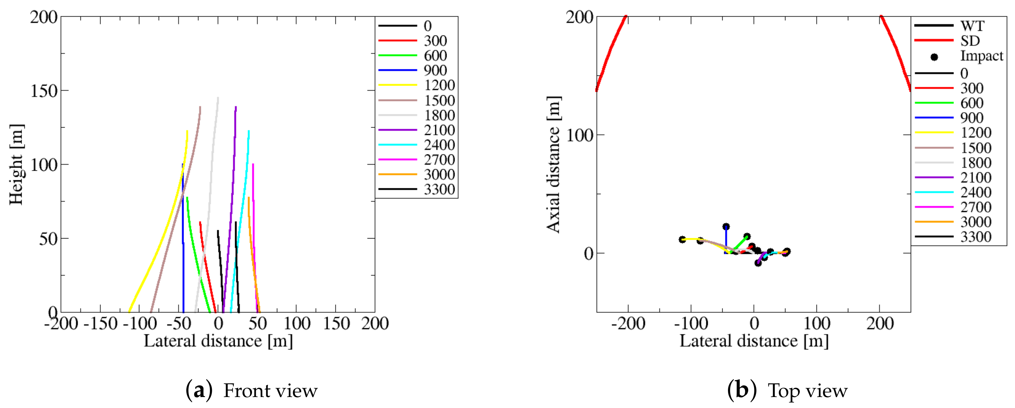
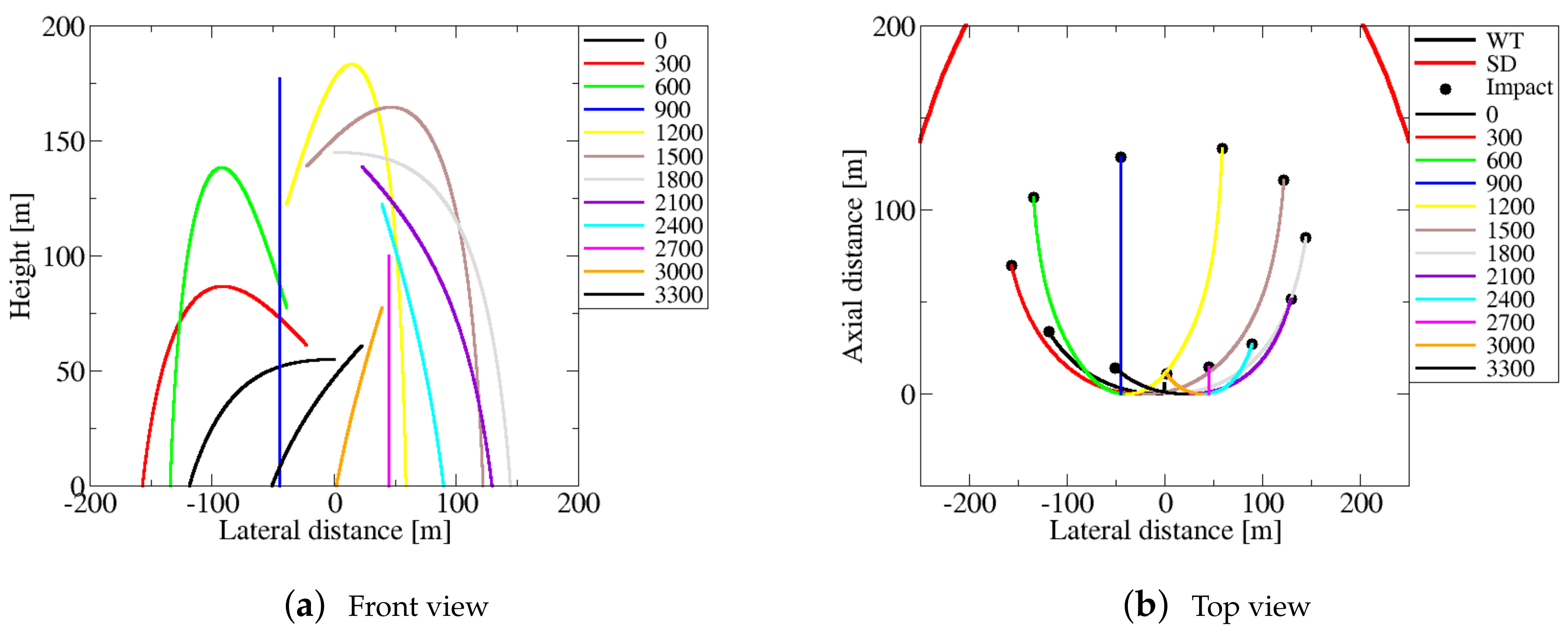
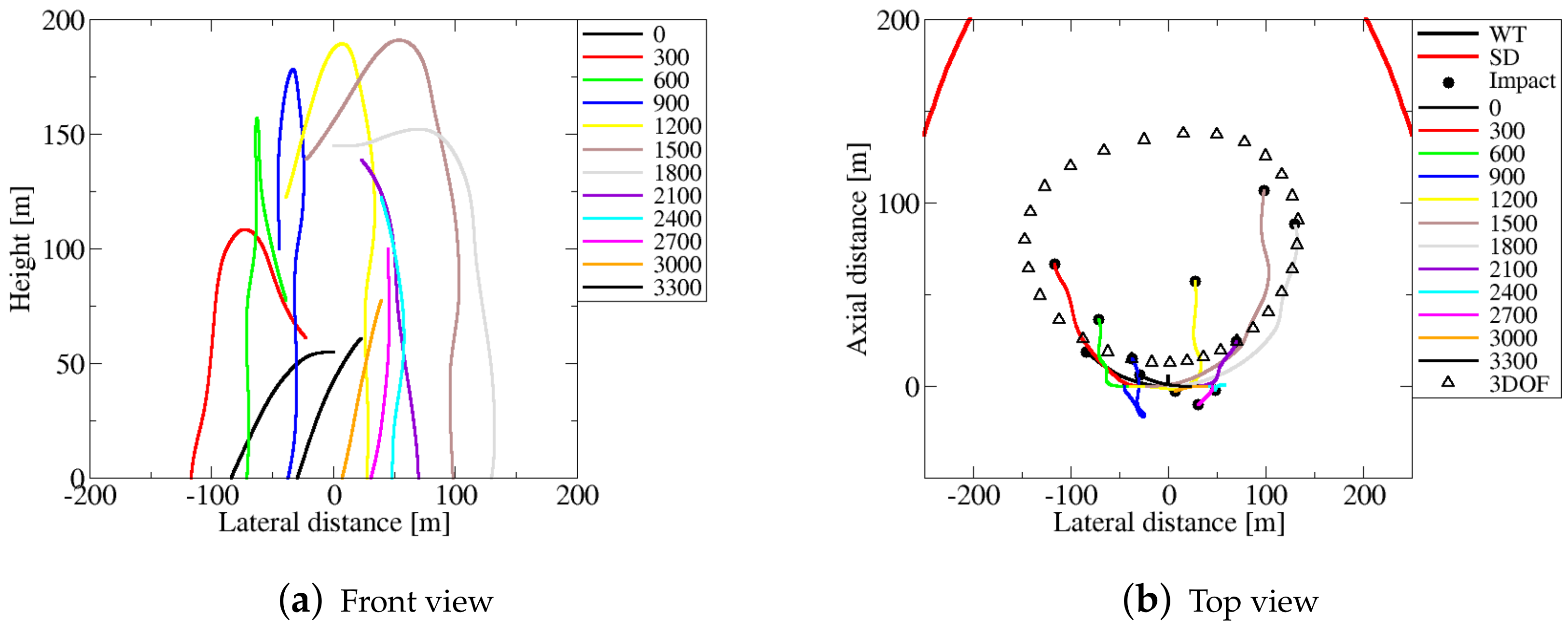
For a more clear view of the trajectories, their front (normal to the rotor disc) and top (normal to the ground) views are plotted in
Figure 3a,b. The ice chunks released at different azimuthal positions are colored differently, the numbers in the legend equal 10 times the release angle in degrees. Due to the lack of side components of the aerodynamic forces, the trajectories are smooth.
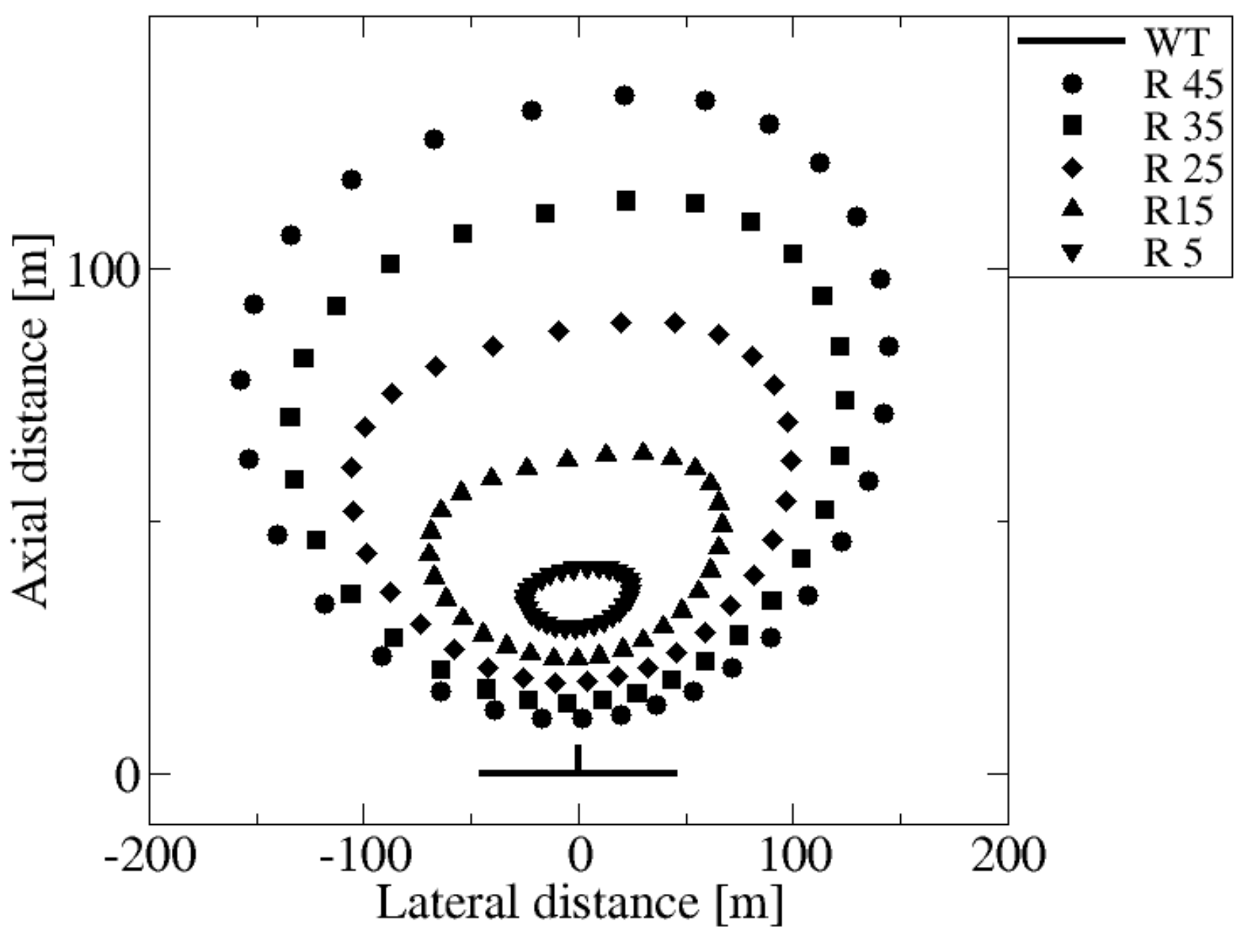
The influence of radial launch position of the ice chunks is visualised in
Figure 4. The investigated range varies between 5 m and 45 m. As expected, ice pieces released at larger radii cover a larger impact area. With increasing radius, the increase in the impact distance for ice pieces released towards the top position of the blade is larger than the corresponding decrease in the distance travelled by ice chunks released when the blades are in the lowest positions.
3.1.2. Influence of Turbine Rotation
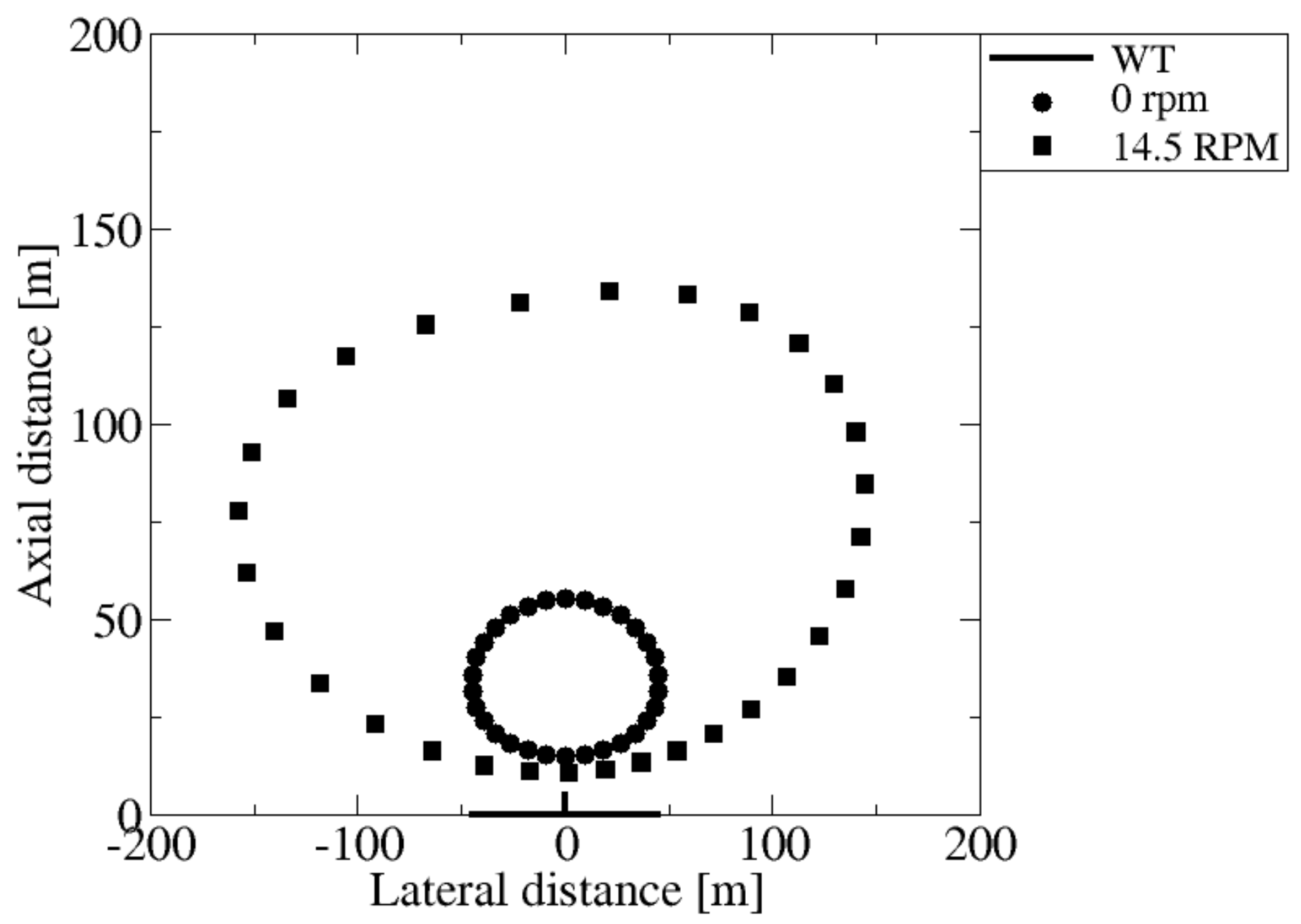
When ice accretion is detected on a wind turbine it is usually stopped to avoid overloading of the parts due to the imbalance and to minimise risks due to ice throw. Thus, it is relevant to study the impact positions of the ice chunks both for rotating and parked rotors.
Figure 5 shows the impact positions for these two cases (the set-up being the same as in the previous subsection). As expected, for the parked wind turbine the impact area is significantly smaller, the width of it is approximately equal to the turbine diameter. The axial extent is approximately half the tower height (50 m) which is still significant if persons have access to the premises.
3.1.3. Influence of Wind Speed
The results presented so far were obtained with a logarithmic wind velocity profile according to Equation (
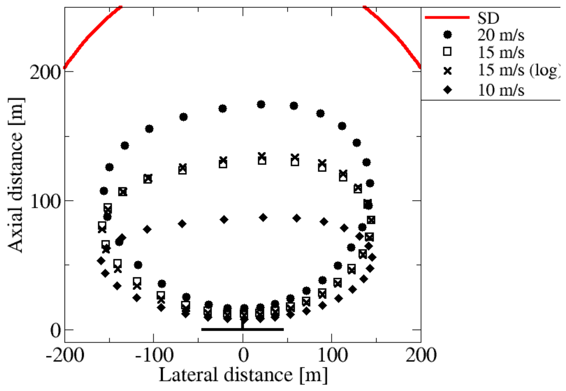
2) resulting in a hub-height wind velocity magnitude of 15 m/s. In order to assess the influence of the wind speed, three more cases have been computed, all three having constant magnitude of the wind speed (not varying by the domain height). The results are shown in
Figure 6 and indicate that the wind speed affects mainly the downstream extent of the impact area, the extent in lateral direction is practically not affected. Again, the trajectories of ice pieces released at higher altitudes are affected more due to the longer flight-time. As it regards the influence of the velocity profile, one can notice a visible, but relatively small difference between the impact locations calculated with a 15 m/s constant wind velocity profile (rectangles) and the impact locations resulting from the logarithmic wind velocity profile having the same magnitude at hub height (crosses). One should note, however, that depending on the state of the atmospheric boundary layer the differences might be larger. In addition, a more accurate description of the velocity field in the wake of the wind turbine is also expected to have a more significant effect on the impact locations.
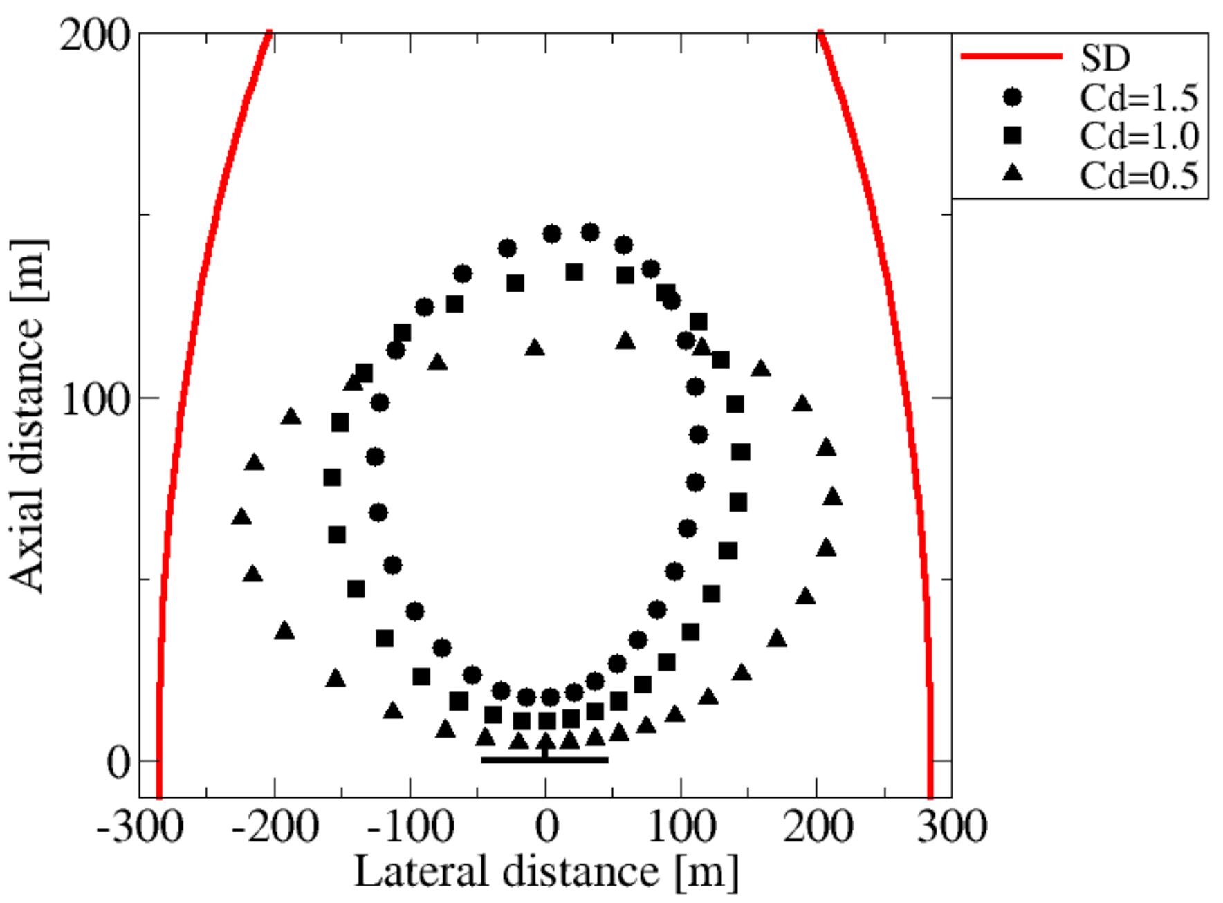
3.1.4. Influence of the Drag Coefficient
From an aerodynamic point of view, the trajectories of the ice pieces are determined by the value of the compound parameter
[
8], i.e., an object having a certain frontal area, a drag coefficient
and a mass of
m = 0.5 kg will have the same trajectory like an object with the same frontal area but
and
m = 1 kg. In order to study the effects of the aerodynamic properties, we chose to keep the frontal area and the mass constant and vary the drag coefficient. The results are summarised in
Figure 7. For lower values of the drag coefficient, the objects interact less with the air and have a tendency to continue on their initial trajectories. As a result, the width of the impact area increases and the axial extend decreases. For low values of
, the impact locations approach the limit of the safety zone in lateral directions.
For large values of the drag coefficient the effect is the opposite. Due to the large drag, the sideways motion of the objects is slowed down, reducing the lateral extent of the impact zone. At the same time, the wind velocity entrains more the objects in the wind direction, the impact zone increasing significantly downstream.
3.2. Trajectories with Object Rotations
From a dynamic point of view there are two major differences between the 3DOF and 6DOF cases. First, in the 3DOF case, only the drag force was accounted for, the lift effects were neglected, thus the aerodynamic force was always acting in the direction of relative velocity. For the 6DOF case, the aerodynamic force components act in three orthonormal directions, allowing for eventual lift effects. The second difference is that, beside the forces, the moments are accounted for as well, thus the attitude of the object is allowed to change during the flight.
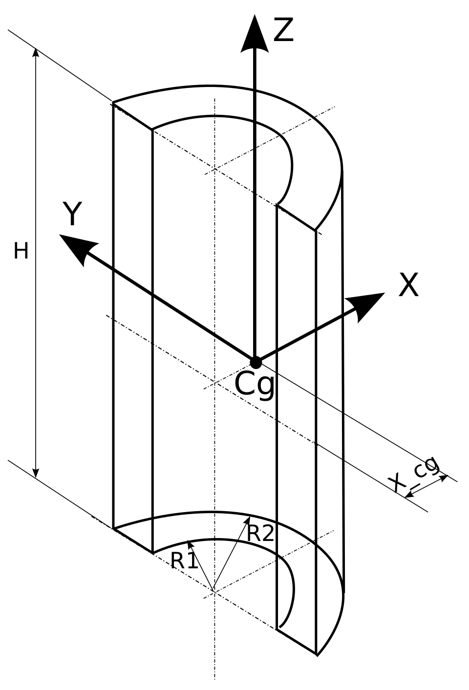
The size and shape of ice chunks detached from wind turbines are largely affected by the atmospheric conditions, the size of the wind turbine and the location where the ice was accreted. Since the treatment of all types of ice shapes would be too exhaustive, for these computations an ice chunk with a ‘C’-shaped cross section was considered (see
Figure 8). This shape is similar to the shape of the ice pieces shed from the leading edge of an airfoil. Since this part of the blade is one of the regions most affected by accretion, it is considered that the shape we opted for is a representative model for a large number of realistic ice chunks. Furthermore, to our knowledge, the literature is focused more on point- and plate-like objects, thus the aerodynamic study of the suggested shape would complement existing findings. The main parameters of the investigated object are listed in
Table 2. The chosen size was deemed to be realistic for the positions close to the tip of a wind turbine blade. The density of the accreted ice varies largely depending on the icing conditions and the amount of trapped air, here a rather compact ice with 900 kg/m
was considered.
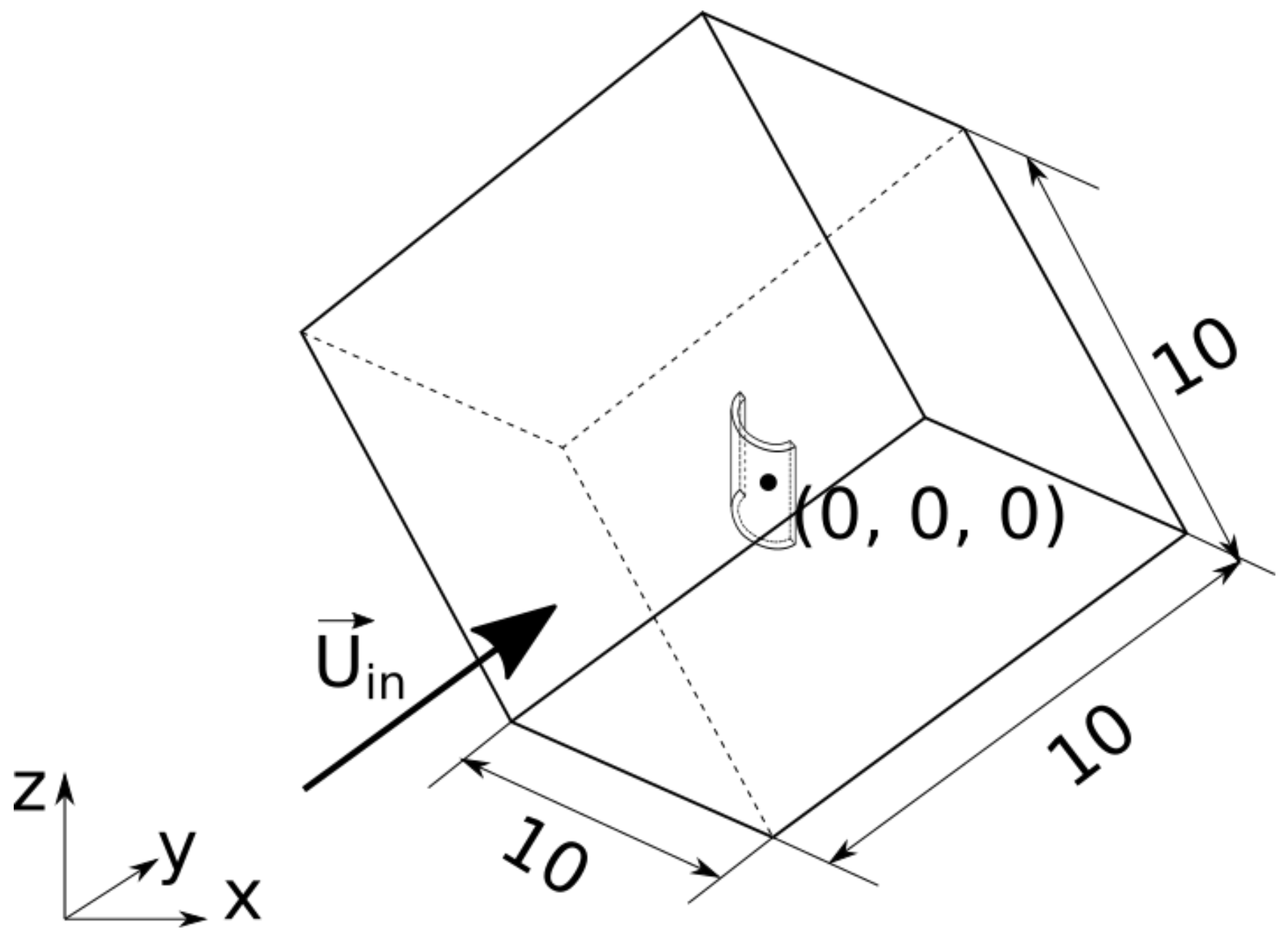
The force and momentum coefficients needed to determine the aerodynamic forces were determined using the simpleFoam solver included in version 4.0 of
OpenFOAM [
9]. The computational domain is sketched in
Figure 9. The mesh was generated by the included
blockMesh and
snappyHexMesh utilities. First
blockMesh was used to generate a 10 × 10 × 10 m base mesh, needed as input for
snappyHexMesh. In the second step, a brick-shaped refinement region of size 1.5 × 0.6 × 0.6 m was generated in the vicinity of the object to improve the resolution. In the third step, the domain has been rotated to have the inlet normal to the desired direction of the relative velocity to be studied. In the last step, the object was removed from the mesh and the mesh was further refined close to the object surface, again using the
snappyHexMesh utility. The values of the aerodynamic forces and moments were integrated using the
forces function object. In this manner, a semi-automated method was developed to compute the force and momentum coefficients in the body-fixed coordinate system having the origin at the center of gravity of the object.
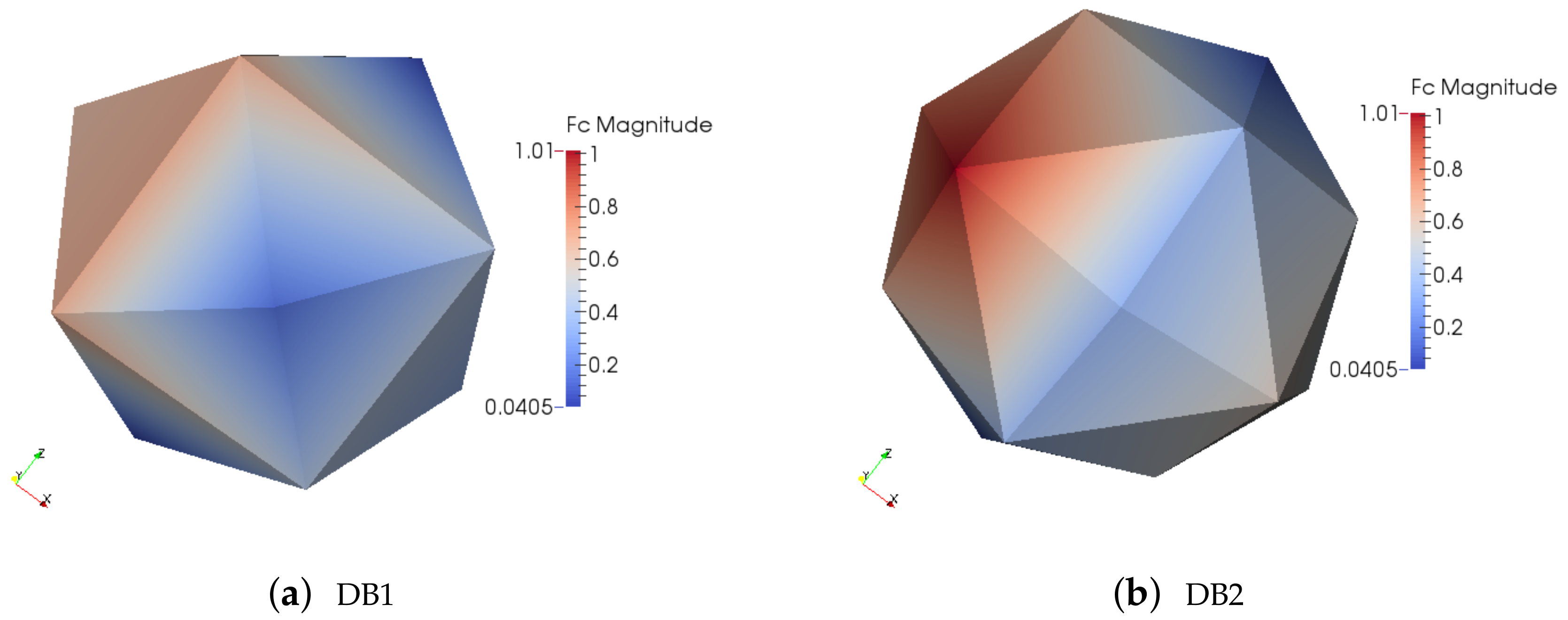
Two force coefficient databases have been generated. For the first database (denoted DB1 in the following), six cases have been computed, the components of the relative velocity for the six cases being listed in
Table 3. Accounting for the symmetry of the object, the obtained coefficients resulted in 14 items in the database. Thus, the resolution of the database is very low and the results should be interpreted only qualitatively.
The second database (DB2) was generated to test the sensitivity of the results. The resolution is only marginally higher (18 vs. 14 datapoints), however, the topology of the datapoints is different. The two datasets are visualized in
Figure 10. The nodes of the triangulated surfaces match the points on the unit sphere (see
Figure 1) where the values of the force and momentum coefficients are pre-computed by CFD. The coloring is carried out by the magnitude of the force coefficient.
Even if the resolution is rather low, the unit spheres are covered uniformly and the databases are deemed to be sufficient to function as proof of concept for the suggested method and to check the sensitivity of the results to the force coefficient database. Further improvement of the accuracy in the interpolated values of the force and momentum coefficients is a matter of carrying out further CFD computations. Such CFD computations being the most time-consuming part (a typical computation needed around 2 h walltime on four cores), one should optimise the direction of the investigated relative velocities to regions with large gradients of the obtained coefficients. Note also that the influence of Reynolds number is not accounted for; this deficiency can also be remedied by adding one more dimension to the database.
3.2.1. Parked Wind Turbine
First the case of a parked wind turbine is investigated.
Figure 11a,b show front (normal to the rotor disc) and top (normal to the ground) views of the computed trajectories for ice chunks released at a radial position of 45 m and varying azimuthal positions. The wind turbine parameters and the wind conditions are the same as for the 3DOF computations and the DB1 database (
Figure 10a) is used.
Figure 11a reveals significant effects of the forces normal to the object trajectories, if only the drag force would have been acting the trajectories would have been vertical lines in this view. The largest effect is observed for the ice released at an angle of 120 degrees (yellow, 0 degree being the lowermost position of the blade tip). The top view of the trajectories (see
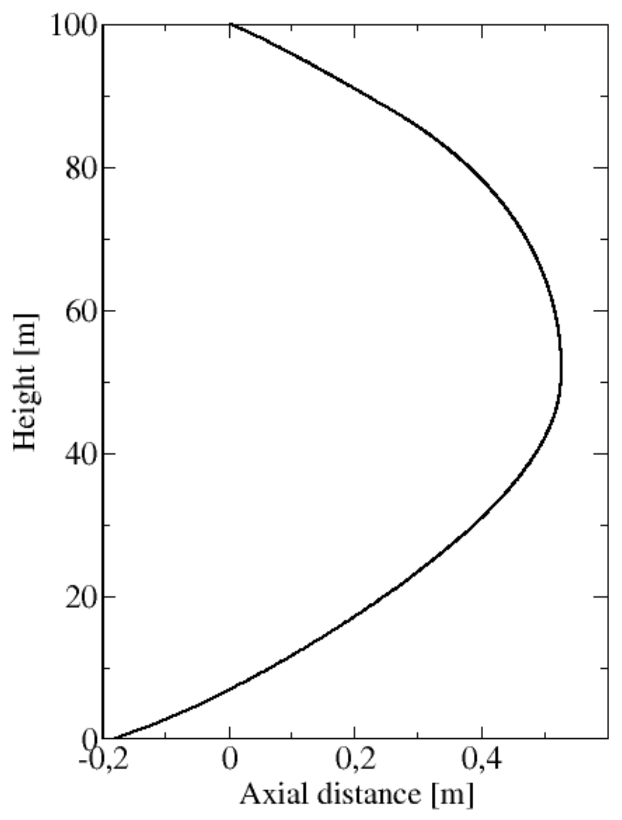
Figure 11b) shows similar effects, compared to the 3DOF cases the impact locations are closer to the tower in the wind direction. Surprisingly, some of the impact locations are even located upstream. To understand this behavior, the side view of the trajectory of such an ice piece is shown in
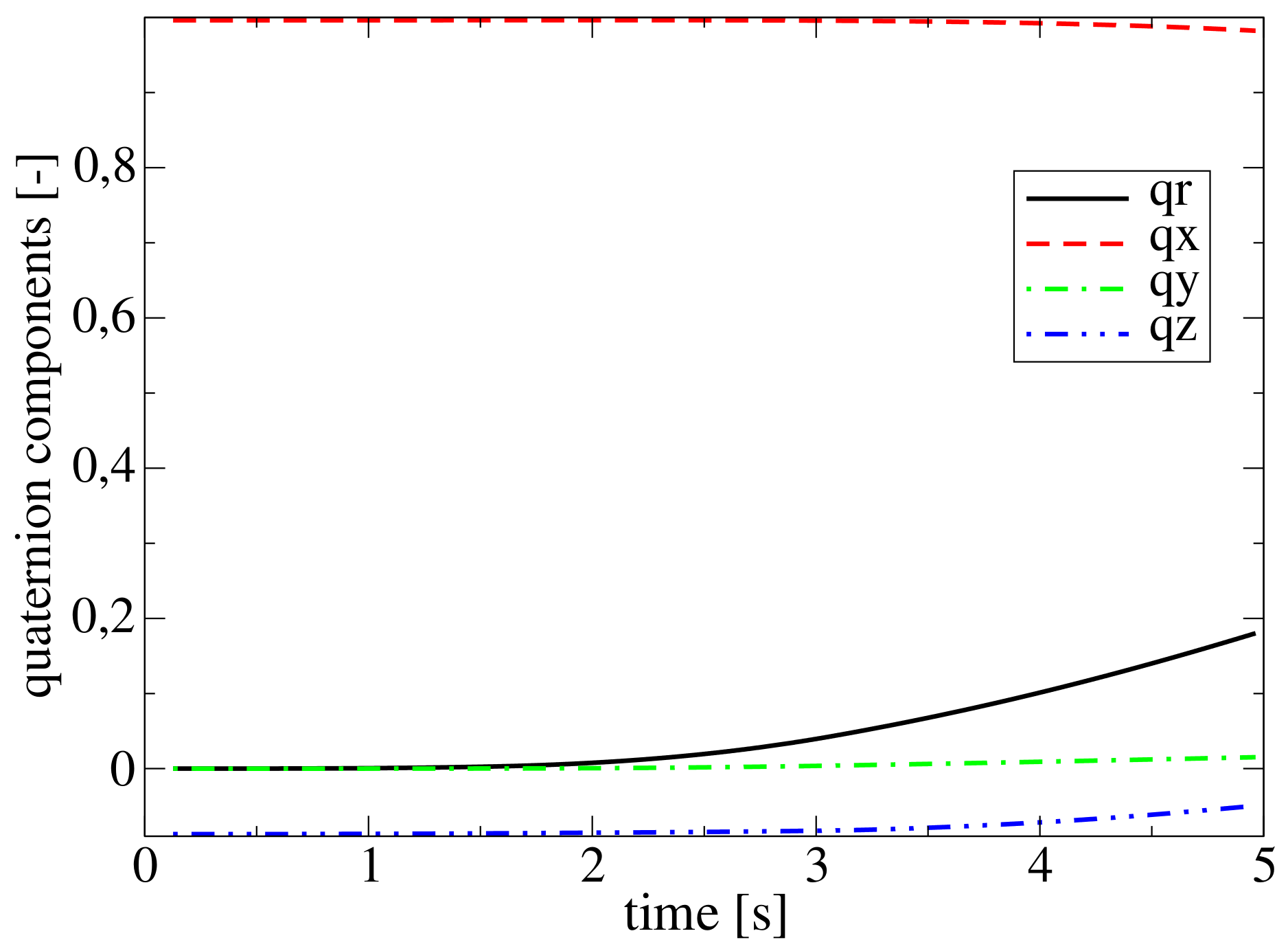
Figure 12. As expected, once the ice chunk is detached from the blade, it begins to travel in the wind direction. At the same time, due to gravity, its vertical velocity magnitude increases, changing the direction of the relative velocity. This effect is further enhanced by the decrease of the wind velocity magnitude as the object approaches the ground. For sufficiently large vertical velocity, the drag of the wind is counteracted and the object changes the direction of the flight. To visualise the changes in the ice chunk orientation, the time evolution of the components of the quaternion (
) are plotted in
Figure 13. As one can observe, the changes in the orientation are relatively small; the object begins to rotate after approximately 2 s. This is probably due to the short flight time and the relatively low magnitude of the aerodynamic moments. For cases with larger magnitudes of the aerodynamic moments or lower magnitude of the moment of inertia tensor, the angular speed of the ice chunk would be larger and there would be a decreased tendency to upstream motion. Furthermore, the wind velocity profile being approximated by a simple logarithmic law, both the high shear in the vicinity of the blades and the eddies due to turbulence are neglected. Accounting for these details of the flowfield would definitely have an impact on the arodynamic forces and moments, and by this on the resulting trajectory.
3.2.2. Rotating Wind Turbine
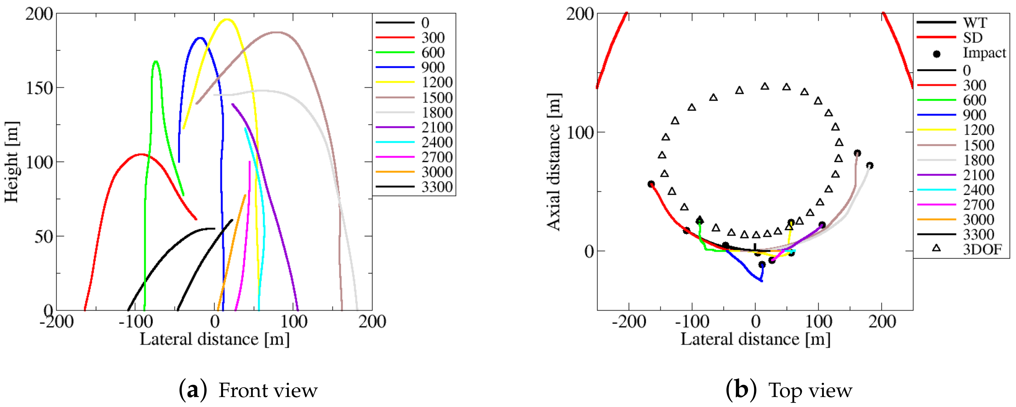
For the case of a rotating wind turbine the results are similar, however, the region of impact positions is larger compared to the region of the parked turbine, see
Figure 14a,b for the front and top views of the trajectories. In the lateral direction, the impact zone increases from ca. (−120 m, 50 m) to ca. (−160 m, 180 m), however, it is important to note that the origins of the ice chunks landing at extreme positions have different azimuthal angles. In the wind direction the impact area increases mainly for large lateral positions, for shorter lateral distances the ice chunks land closer to the tower even in the wind direction. Compared to the 3DOF computations (
Figure 3a,b) the trajectories are much more irregular due to the three-dimensionality of the aerodynamic forces and the attitude changes of the flying objects.
As one can observe, the impact positions determined with 3DOF computations (marked with triangles in
Figure 14b) deviate significantly from the ones predicted by the 6DOF approach (filled circles). One reason for the discrepancies is the fact that in the 3DOF computations, a constant value of
has been used, this value being based on the average magnitude of the force coefficients from the database. In the 6DOF computations, the value of the force coefficient changes in time depending on the orientation of the object. Another reason for the discrepancies is that in the 3DOF computations, only the forces in the direction of the relative velocity are accounted for.
3.2.3. Sensitivity to the Force Coefficient Database
In order to assess the sensitivity of the results to the underlying force coefficient database, the trajectory computations of the ice chunks released from the rotating wind turbine have been repeated using the database DB2 (
Figure 10b). The front and top views of the ice chunk trajectories are shown in
Figure 15. Comparing to the DB1 results (
Figure 14), one can notice a significant influence of the force coefficient database on the predicted trajectories. In the case of DB2, the impact area is narrower but more elongated than in the DB1 case. This behavior is probably due to the fact that DB2 includes a datapoint with a larger magnitude of the force coefficient (see
Figure 10), thus leading to a similar effect as increasing the drag coefficient in the 3DOF case (see
Figure 7). The discrepancies between the impact positions determined by 3DOF (triangles) and 6DOF (circles) approaches are slightly smaller than in the case of DB1, but the differences are still significant. The observed high sensitivity of the results suggests that a good quality database is crucial to assure the reliability of the impact position predictions.
4. Conclusions
A method was implemented to compute the trajectories of ice pieces released from rotating and parked wind turbines. First, the method commonly used in the literature (accounting only for translation) has been implemented and the sensitivity of the trajectories to several controlling parameters (wind speed, turbine rotation, azimuthal and radial release positions and ice drag coefficient) has been evaluated. The results agreed well with data reported previously in the literature.
In the second part, the objects were also allowed to rotate during the flight. The aerodynamic forces and moments have been precomputed a-priori using CFD computations and their normalised values have been stored in a database. This database has been used in the trajectory computations to estimate the instantaneous forces and moments acting on the object during the flight, depending on the instantaneous relative velocity. Although the accuracy of the 6DOF computations is limited due to the relatively coarse resolution of the database, the results revealed that the forces are normal to the trajectories and the changes in the object attitude might have significant effects on the ice trajectories. Furthermore, the results revealed that the predicted trajectories are very sensitive to the quality of the force coefficient database used for the 6DOF computations. Since all predicted impact locations were well within the limits prescribed by Equation (
1), the investigated parameters are not expected to influence the safety when the safety distance prescribed by Equation (
1) can be respected. However, if one cannot afford the traditionally-prescribed safety distance, or if one needs to investigate incidents, 3D effects cannot be neglected any more.
Performance-wise, the suggested method is located in-between traditional 3DOF trajectory computations and full-CFD simulations of the flying objects. Due to the need for force and momentum coefficient databases, the computational cost of this method is significantly higher than the cost of pure 3DOF. Nevertheless, once a database is generated, it can be reused for similar objects and then the additional cost of interpolating coefficients from the database vs. assuming constant values of the coefficient is minimal and probably well motivated by the additional gain of accuracy. Full CFD computations of the flying objects is estimated to be at least one or two orders of magnitude more demanding computationally. Due to the large interval of scales which need to be captured and the relatively long time intervals (compared to the timescale of the flow around the object), a 3D computation of the flow-field including both the wind turbine and the flying ice chunks would require unreasonably large resources. Thus, a more realistic approach would be CFD computations of the flow in a domain moving together with the ice chunk, however, that approach would still be significantly more demanding than the approach suggested herein.
The accuracy of the suggested method can be increased primarily by increasing the resolution of the database used to store the aerodynamic forces. In addition, even more realistic wind velocity fields, by including a wake model or by precomputing the velocity field by CFD, would also enhance the quality of the results. The suggested method is easily applicable to other kinds of trajectory computations as well, for example, to assess the trajectory of flying debris in heavy storms.
Author Contributions
Conceptualization, R.-Z.S. and J.R.; Investigation, R.-Z.S. and A.L.; Software, R.-Z.S. and A.L.; Supervision, J.R.; Writing—original draft, R.-Z.S.; Writing—review & editing, R.-Z.S., A.L. and J.R.
Funding
This research was partially funded by ÅForsk grant number 18-535.
Acknowledgments
The CFD computations were performed on resources provided by the Swedish National Infrastructure for Computing (SNIC) at Lund University (LUNARC).
Conflicts of Interest
The authors declare no conflict of interest.
Nomenclature
| d | safety distance [m] |
| D | rotor diameter [m] |
| aerodynamic force vector [N] |
| gravitational acceleration vector [m/s] |
| h | altitude [m] |
| surface roughness height [m] |
| H | hub height [m] |
| moment of inertia tensor [kg m] |
| von Kármán constant [-] |
| m | ice mass [kg] |
| aerodynamic moment vector [N m] |
| friction velocity [m/s] |
| wind speed [m/s] |
| velocity vector [m/s] |
| angular velocity vector [rad/s] |
References
- Laakso, T.; Baring-Gould, I.; Durstewitz, M.; Horbaty, R.; Lacroix, A.; Peltola, E.; Ronsten, G.; Tallhaug, L.; Wallenius, T. State-of-the-Art of Wind Energy in Cold Climates; VTT: Espoo, Finland, 2010. [Google Scholar]
- LeBlanc, M. Recommendations for Risk Assessments of Ice Throw and Blade Failure in Ontario; Technical Report; Garrad Hassan Canada Inc.: Vancouver, BC, Canada, May 2007. [Google Scholar]
- Cattin, R.; Russi, M.; Russi, G. Four years of monitoring a wind turbine under icing conditions. In Proceedings of the International Workshops on Atmospheric Icing of Structures (IWAIS XIII), Andermatt, Switzerland, 8–11 September 2009; pp. 6–10. [Google Scholar]
- Seifert, H.; Westerhellweg, A.; Kröning, J. Risk analysis of ice throw from wind turbines. In Proceedings of the BOREAS, Pyhä, Finland, 9–11 April 2003; pp. 1–9. [Google Scholar]
- Tammelin, B.; Cavaliere, M.; Holttinen, H.; Morgan, C.; Seifert, H. Wind Energy Production in Cold Climate (WECO); Technical Report; Finnish Meteorological Institute: Helsinki, Finland, 1998. [Google Scholar]
- Morgan, C.; Bossanyi, E.; Ashton, L. Wind Turbine Icing and Public Safety—A Quantifiable Risk? In Proceedings of the Wind Energy Production in Cold Climates (Boreas III), Saariselkä, Finland, 19–21 March 1996. [Google Scholar]
- Dalsgaard, J.; Nørkær, J.; Kjærgaard, J. Risk assessment of wind turbines close to highways. In Proceedings of the EWEA 2012 European Wind Energy Conference and Exhibition, Copenhagen, Denmark, 16–19 April 2012. [Google Scholar]
- Biswas, S.; Taylor, P.; Salmon, J. A model of ice throw trajectories from wind turbines. Wind Energy 2012, 15, 889–901. [Google Scholar] [CrossRef]
- OpenFOAM. Available online: http://www.openfoam.org (accessed on 26 February 2019).
© 2019 by the authors. Licensee MDPI, Basel, Switzerland. This article is an open access article distributed under the terms and conditions of the Creative Commons Attribution (CC BY-NC-ND) license (https://creativecommons.org/licenses/by-nc-nd/4.0/).


