1. Introduction
Since the development of the nonlinear harmonic (NLH) method by He and Ning [
1], various frequency domain methods have been presented in the literature that allow for an efficient computational fluid dynamics (CFD) prediction of time-periodic unsteady flows in turbomachinery, in particular the so-called harmonic balance (HB) method [
2,
3]. The fact that the flow residuals in an HB solver are evaluated at discrete time instants means that existing routines from a steady solver can be employed and the development is greatly simplified, even if robust solution methods and accurate blade–row interfaces for HB are still challenging. In the NLH approach, the development of the cross coupling terms between the harmonics can be quite intricate [
4]. Therefore, only the nonlinear coupling through the zeroth harmonic by deterministic stresses is usually taken into account. The NLH approach, however, has no limitations as to the choice of frequencies. The extension of harmonic balance solvers for multiple base frequencies is the subject of ongoing research [
5,
6,
7].
Similar to the issue of multiple base frequencies is the prediction of rotational aperiodicities in the time-averaged flows, which, in the terminology of frequency domain solvers, can be viewed as additional harmonics with zero frequency and non-zero interblade phase angle. These occur, e.g., when rotor–rotor or stator–stator interactions are to be simulated. He et al. [
8] have shown that the NLH approach can be carried over in a straightforward manner to zero-frequency harmonics. As for the harmonic balance method, Subramanian et al. [
5] use a small, fictitious shift of the rotation speed and obtain a configuration with several base frequencies. The aim of this paper is to demonstrate that the
harmonic set approach presented by the authors [
7] is capable of accurately predicting rotationally asymmetric time-averaged flows, without introducing fictitious rotational speeds.
The paper is organised as follows. The harmonic set concept used in the present HB solver is summarised and its generalisation to zero-frequency harmonics is explained. It is shown that the discrete Fourier transform with respect to the passage index leads naturally to a harmonic balance formulation of the possibly aperiodic time-averaged flow. One thereby introduces a generalised notion of sampling points for zero-frequency modes that correspond to circumferential positions rather than time instants. It is shown that, if the sampling points correspond to the true positions of the blades (or vanes), then, in contrast to the method of He et al., the zero-frequency harmonic balance system is derived without using simplifications such as linearisation hypotheses. An academic test case is used to demonstrate the accuracy of the method. Finally, the method is applied to predict the impact of inlet distortions in a fan stage. For this configuration, the results are validated against unsteady simulations in the time domain and HB simulations on full annulus configurations.
2. The Harmonic Balance Method
The methods described below are integrated into the DLR flow solver TRACE [
9,
10]. TRACE has several solver modes for the steady, unsteady, linearised, and adjoint RANS equations. In recent years, it has been extended to solve the HB equations in an alternating frequency time domain (AFT) framework [
7]. The underlying spatial discretisations employed here are based on the finite volume approach. We use Roe’s upwind scheme [
11] in combination with a MUSCL extrapolation to achieve second order accuracy [
12]. In this work, a van Albada type limiter is employed to smoothen the solutions in the vicinity of shocks [
13].
The HB solver is based on the concept of so-called
harmonic sets. A harmonic set is defined by a base frequency
f, a base interblade phase angle
and a set of harmonic indices
. Each harmonic index
thus corresponds to a harmonic with angular frequency
,
, and interblade phase angle
. There may be several harmonic sets, and different harmonic sets may have some harmonics in common. Keep in mind that a harmonic is determined by both its frequency and its interblade phase angle. Thus, when dealing with two harmonic sets with base frequencies
and interblade phase angles
, there may exist integers
such that both
and
. Note that, in the solver, these harmonics are then treated as one harmonic flow field. In the following, denote by
the
i-th harmonic set and the union of all harmonics sets, respectively. The reconstruction in time reads
where
denotes the Fourier coefficient associated with the angular frequency
and interblade phase angle
. The harmonics can be defined in two steps. First, the full annulus time harmonic is given by
where
for
and
for
. Then, the discrete (complex) Fourier transform with respect to the passage index yields
where
L denotes the number of passages.
The HB method in TRACE is formulated in the frequency domain, i.e., it solves
for all harmonics
. Here, the second term denotes the discrete Fourier transform of the flow residual evaluated at an appropriate number of sampling points. When generalising a single base frequency harmonic balance code to multiple base frequencies, the crucial difficulty is to define the discrete forward Fourier transform. The HB formulation in TRACE uses, for each base frequency
, equidistant sampling points
The number of sampling points
is set to
. Here, the number of sampling points per period for the highest harmonic,
, must be at least three in order to ensure that the highest harmonic is smaller or equal to the Nyquist frequency.
is the value defined by Orszag [
14] to guarantee that taking products of two harmonics in
does not yield a mode that is indistinguishable from some original harmonic in
(aliasing). The harmonic balance residual for a mode
with respect to a certain harmonic set is now defined as
Here,
denotes the unsteady flow field using all harmonics of
, i.e., the sum in Equation (
1) is taken over the modes in
. The multiple harmonic set approach is to approximate the
-harmonic of the residual by a weighted sum
where the HB residual for each harmonic set is computed with an individual, appropriate set of equidistant sampling points. The weights
are assumed to satisfy
where
is the characteristic function of the set
. This means that, in Equation (
3), a harmonic may be accounted for more than once, but its weights will add up to 1. As explained in [
7], the resulting total HB residual is accurate up to second order terms, i.e., the error can be estimated by
where
denotes the exact Fourier coefficient of
, viewed as an almost periodic function. The coupling terms within one harmonic set are even third order accurate, cf. [
7].
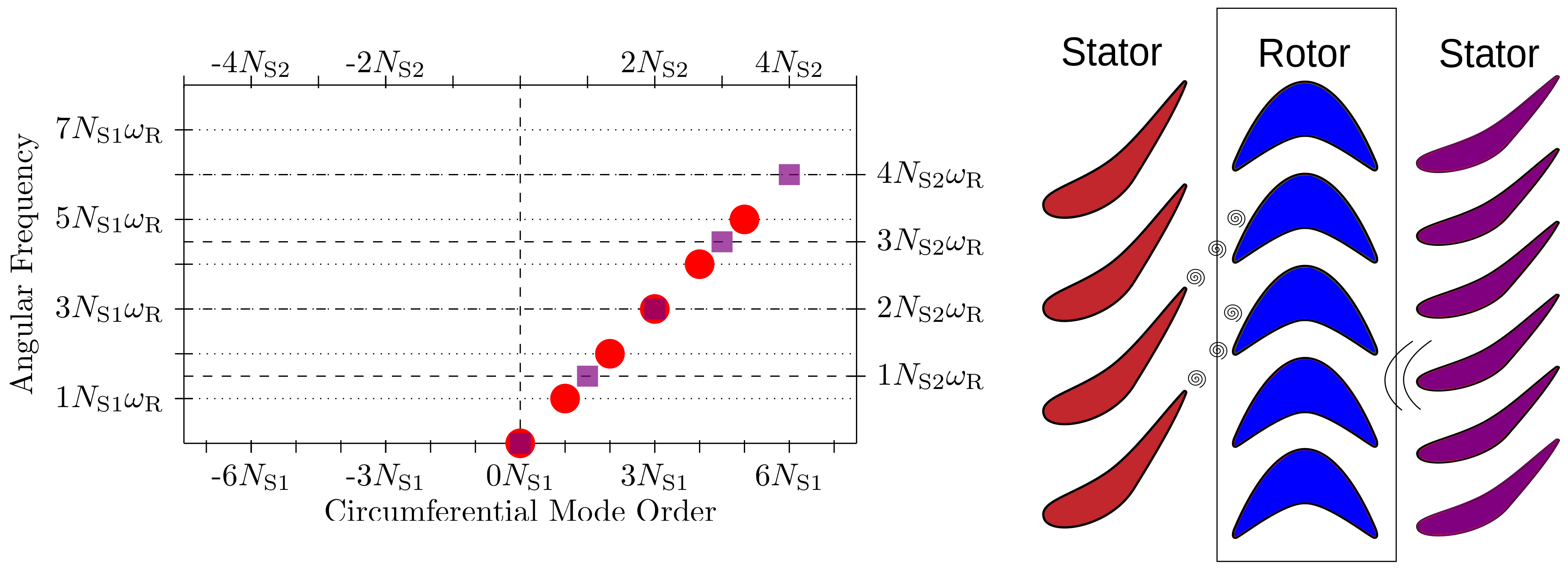
2.1. Example 1: Up- and Downstream Disturbances within a Component
To illustrate the concept of harmonic sets, consider the disturbances caused by up- and downstream stators with and blades on a rotor with blades.
The disturbances in the rotor can be represented by the harmonics sets
which are depicted in
Figure 1 by red and violet dots. Here, the circumferential mode order is plotted instead of the interblade phase angle. Keep in mind that, since two angles that differ by a multiple of
are identified, mode orders
for which
is a multiple of
, are represented by the same mode in
.
Note that, since the relative rotational speeds are equal, the disturbances lie on the same line. and have a mode in common if there are integers such that the -th harmonic is in and , i.e., equals the vane count ratio. These considerations carry over almost verbatim to a rotor–stator–rotor configuration.
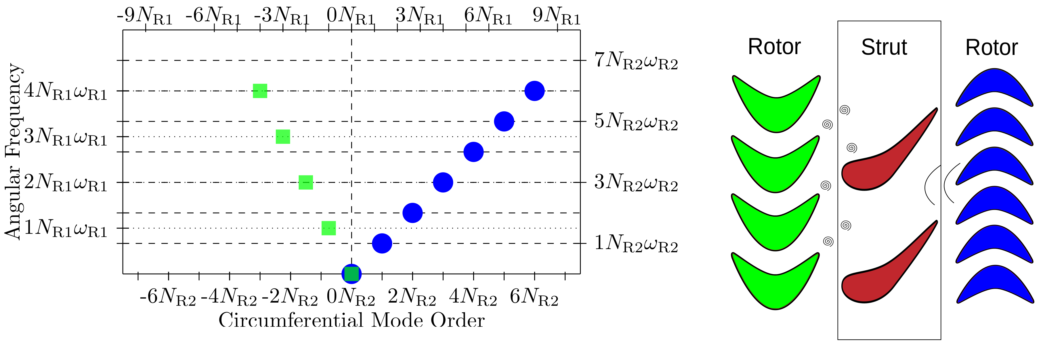
2.2. Example 2: Up- and Downstream Disturbances with Different Relative Rotational Speeds
Consider a stator between two rotors with different wheel speeds, e.g., a mid turbine frame consisting of
struts that are arranged between high-pressure and low-pressure turbines. The disturbances coming from the neighbouring rotors can be represented using harmonic sets with angular base frequencies
and interblade phase angles
. Observe that the shaft speeds,
,
are no longer equal in this case. Typical harmonic sets are depicted in
Figure 2. This example is a configuration with a turning strut between high and low pressure turbine blade rows. Here, the high and low pressure components are contra-rotating.
Note that, in
Figure 2, a point in the half planes corresponds to a
mode rather than to a
harmonic. Two modes with different circumferential mode orders
are contained in one harmonic
if
Hence, two modes in these plots correspond to the same harmonic if and is a multiple of . Therefore, even for unequal rotor speeds, the direct disturbance harmonic sets may intersect.
Furthermore, note that the method of harmonic sets does not resolve possible modes that are generated by the interaction of different harmonic sets. Due to the nonlinear terms in the flow equations, two modes in the plots of
Figure 2 will generate modes that correspond to integer linear combinations of the vectors in the half plane.
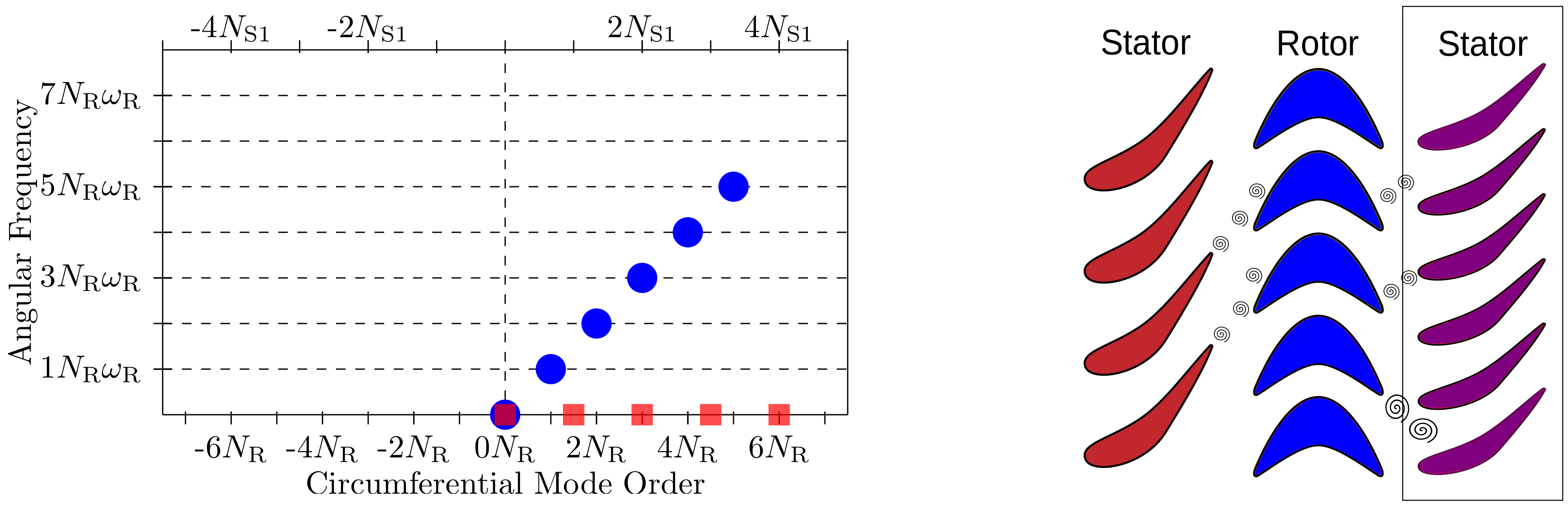
3. Zero-Frequency Harmonics
The aim of this section is to demonstrate that the harmonic set approach can be carried over to the case where a base frequency vanishes. This allows one to simulate rotor–rotor or stator–stator interactions on computational domains that consist of a single passage per row. As an example, consider a blade–row configuration with blade counts
,
,
and rotor speed
. Then, the transmission and scattering of the wakes of the first stator in the rotor will cause a spectrum of modes
in the second stator with
where
,
. These modes can be resolved by harmonics with angular frequency
and interblade phase angle
In particular, if
is not an integer mutliple of
, there will be modes with zero frequency but non-zero
m and thus non-zero
. Their interblade phase angles are
, where
k is the integer corresponding to the
k-th higher harmonic of the original wake. Since, for zero-frequency harmonics, the disturbances with interblade phase angles
and
coincide (their harmonic flow fields are simply complex conjugates of each other), it suffices to consider positive interblade phase angles. Therefore, it follows that one can represent the resulting aperiodicity in Stator 2 by zero-frequency harmonics with interblade phase angle
The resulting harmonic set, together with a harmonic set for the downstream disturbance of the rotor, is depicted schematically in
Figure 3. For a harmonic set of the form
the reconstructed flow field solves the steady flow equations in all passages if and only if
for all passage indices
. For this, it suffices to require Equation (
5) for the passage indices
. The crucial observation is that this is equivalent to the standard harmonic balance equation (Equation (
2)) for
. Moreover, the notion of a sampling point
is replaced with the corresponding
sampling phase. Instead of
for
, one sets
This implies that the flow, reconstructed at the
l-th sampling point,
equals the mean flow in the
l-th passage. This approach is therefore exact in that, for the time-averaged flow, it is equivalent to the full annulus nonlinear steady equations.
Elementary algebra shows that the corresponds to an equidistant distribution of points in the interval . To reduce the computational costs, however, one can also approximate the aperiodicity by a harmonic set with higher harmonics and use equidistant sampling phases . It should be pointed out that the interactions with other harmonic sets are not incorporated in this approach. In particular, the influence of indexing or clocking on the propagation of unsteady disturbances is not captured.
3.1. Mode Coupling and Solution Method
The blade row coupling method outlined in [
7,
15] is based on circumferential Fourier coefficients. In this algorithm, modes with equal frequency but different interblade phase angles can be distinguished. The generalisation to zero frequency modes is therefore straightforward. Similarly, the implicit time-marching procedure to solve the resulting harmonic balance systems is formulated on the basis of decoupled complex linear systems for the harmonics and thus generalises to the case
.
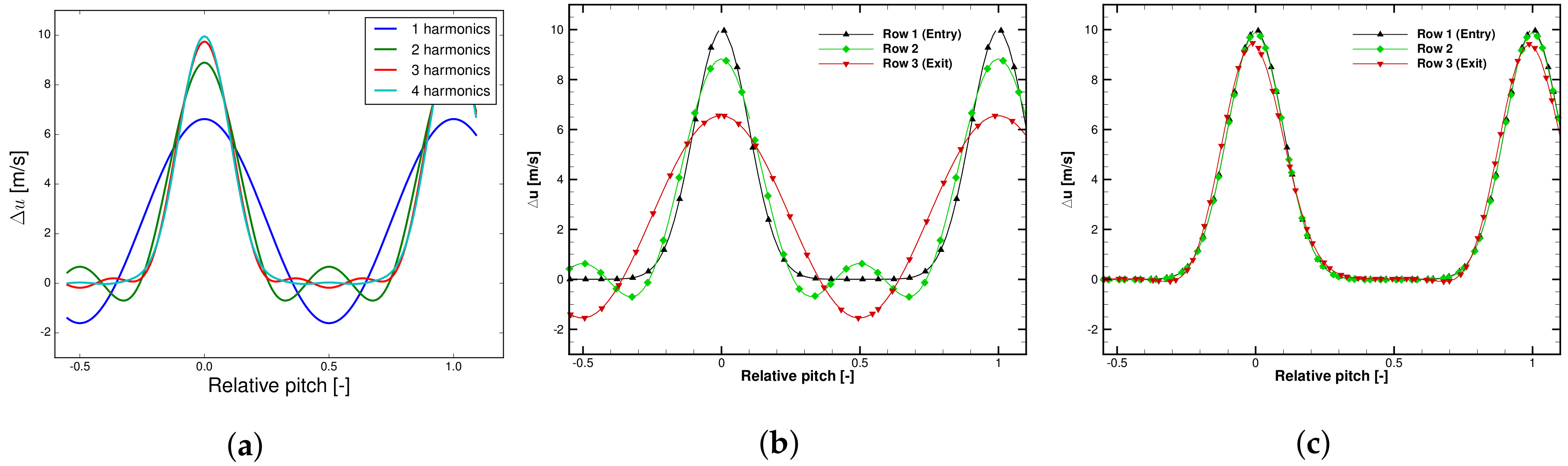
3.2. Numerical Example
The harmonic set approach for zero-frequency harmonics is illustrated by means of a numerical test case consisting of three two-dimensional duct segments through which an artificial jet-like axial velocity disturbance,
with amplitude
m/s is propagated. The duct segments consist of empty cylinder segments and mimic a stator–rotor–stator configuration. The Fourier coefficients of
can be computed from the Fourier transform of the Gaussian distribution and are given by
where
m is an integer multiple of
. The unsteady velocity and its reconstruction with up to four harmonics are depicted in
Figure 4a. The harmonic balance solver is tested with two harmonic set configurations, summarised in
Table 1. The results of the harmonic balance computations are plotted in
Figure 4b,c, which show the velocity disturbance at the entry (Row 1), the “rotor” exit (Row 2) and the second “stator” exit (Row 3). The plots for the limited harmonic set (
Figure 4b) show that, as expected, the resulting disturbance at the rotor exit corresponds to the reconstruction with two harmonics, whereas, at the second stator exit, it merely consists of the first harmonic. It can be seen that the velocity disturbance is propagated very accurately if it is fully resolved (
Figure 4c). It should be pointed out that the harmonic set in the rotor filters the modal content of the disturbance. Hence, it is necessary to resolve the unsteady disturbance accurately in the rotor.
4. Fan Simulation with Inlet Distortion
In the following, the above methodology is applied to predict the impact of inhomogeneous inflow conditions on a fan stage. The motivation for such a CFD simulation is due to the fact that boundary layer ingesting propulsion systems offer considerable advantages regarding system efficiency and mission fuel burn [
16]. Whereas in these configurations the rotor is subject to a periodic variation of the inflow condition, the stator has a fixed relative position with respect to the inflow distortion and therefore exhibits indexing.
Here, a modern low pressure fan for a civil aero-engine, derived from a previous DLR design study [
17], is used. The fan features a meridional inflow Mach number of
and a design total pressure ratio of
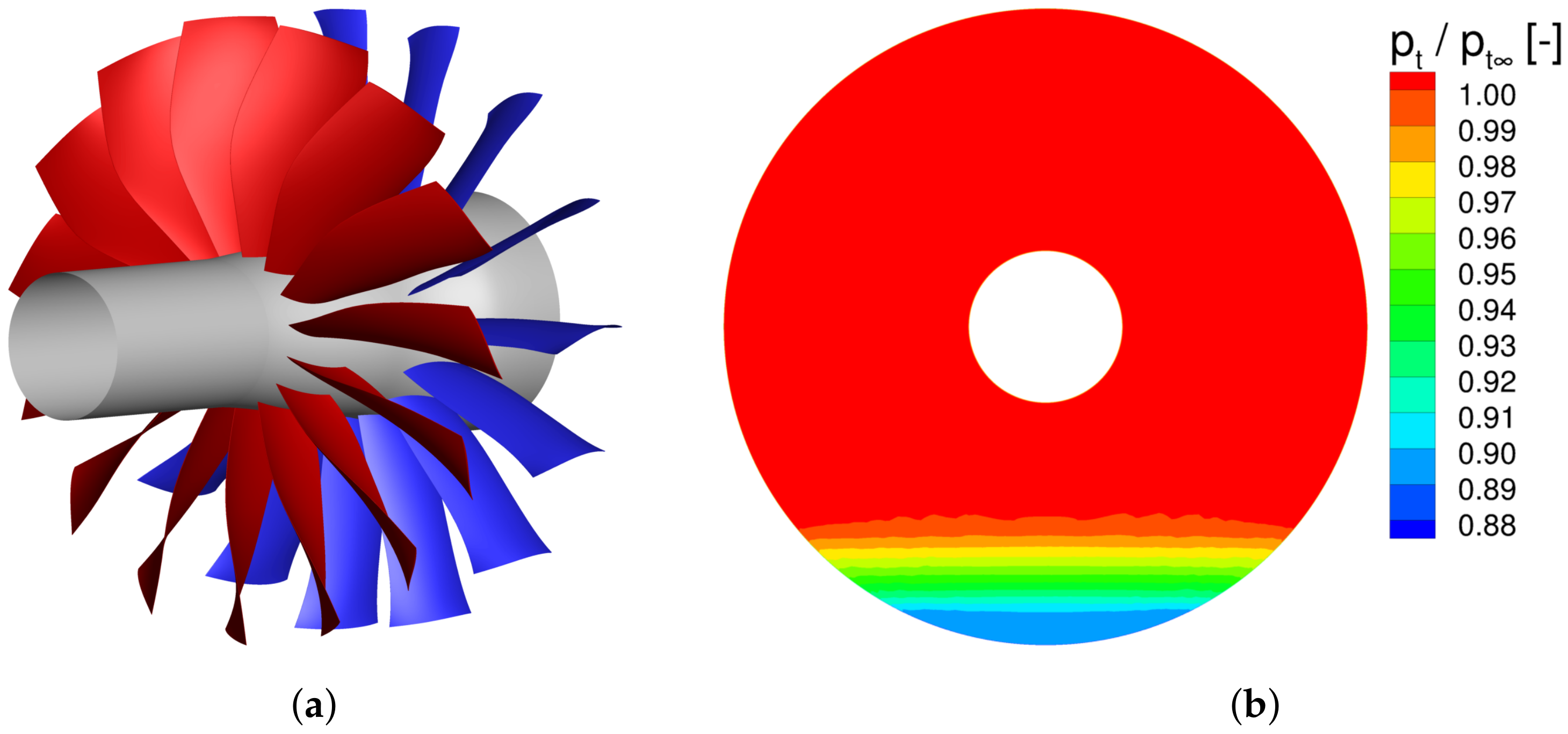
. Both rotor and stator are comprised of 15 blades/vanes. The inflow distortion (depicted in
Figure 5b) models an ingested boundary layer of an airplane fuselage and is similar to the ones presented by [
18,
19]. It has the form of an ideal turbulent boundary layer that covers
of the inlet duct height in the lower part of the annulus. The highest total pressure distortion in this boundary layer is
relative to the far-field inflow total pressure.
For this numerical study, a setup consisting of three domains is used: inlet duct, fan rotor and fan stator (see
Figure 5a). To obtain reference results for the HB solver, a time domain full annulus simulation is performed using the BDF2 time integration scheme with 64 time steps per rotor pitch rotation. Two harmonic balance simulations are run, both using a full annulus inlet duct and a single rotor passage. The setups differ in the stator row where the first one consists of a full annulus while the second one uses a single passage mesh in combination with an additional zero-frequency harmonic set. Harmonic convergence studies have shown that a reasonable agreement between time-integration and HB results can be expected as long as eight harmonics are used for the downstream disturbances. For the upstream disturbances, four harmonics have proven to be sufficient. The meshes used are suitable for wall function boundary layer models and are, up to the number of passages, identical for all setups. The numbers of cells and the computational efforts for the different setups can be found in
Table 2. Compared to both time-domain and HB full annulus simulations, the harmonic balance setup with a single passage stator shows a significant reduction in computational time. It should be pointed out, however, that the authors expect further speed-ups of the HB simulations from the use of fast Fourier transformations. In contrast to single passage HB setups, the numerical computation of the circumferential Fourier coefficients at the blade row interfaces can turn into a serious bottleneck when many passages are simulated.
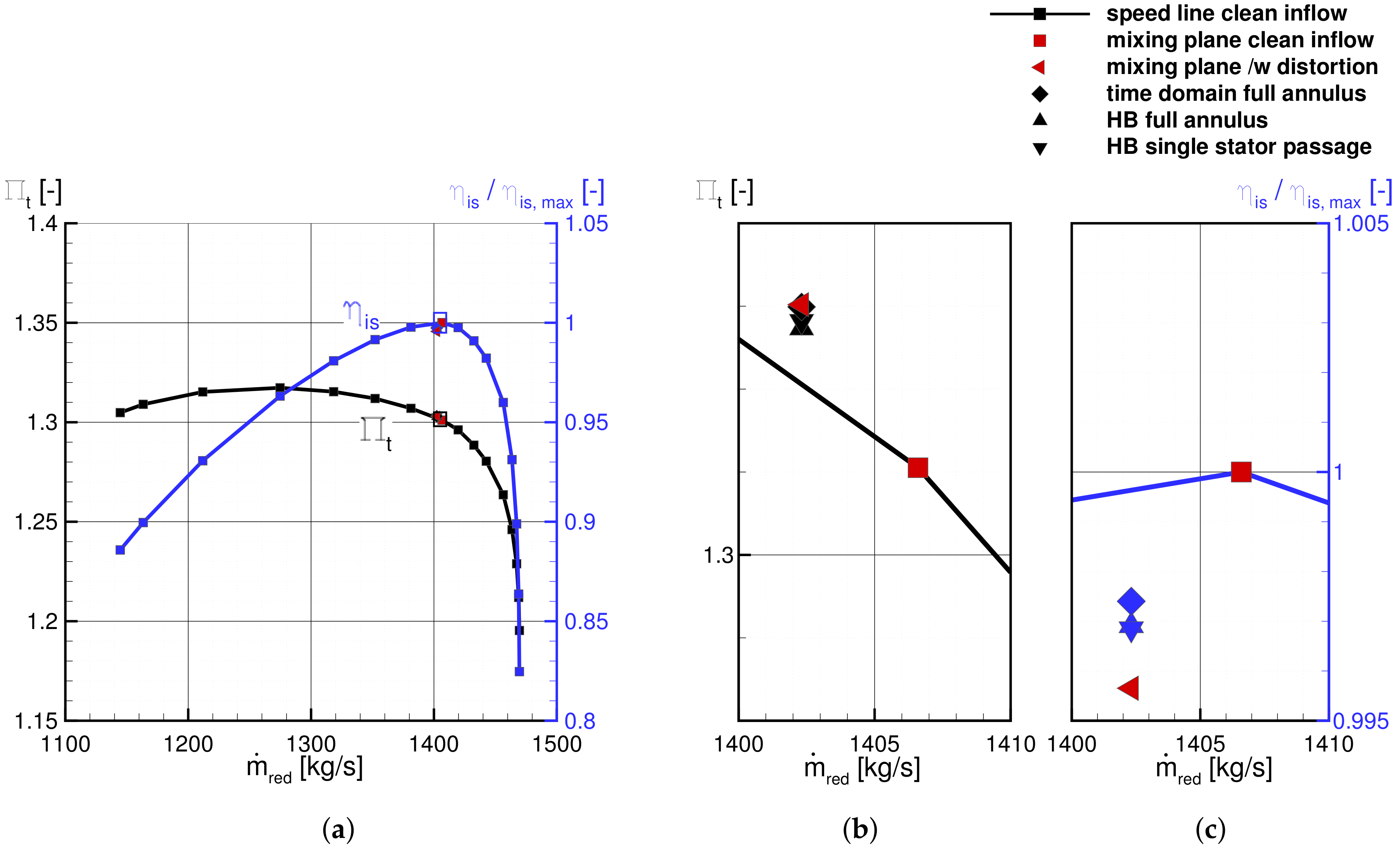
Figure 6a shows the design characteristic with undistorted inflow, together with one operating point under distorted inflow conditions, as predicted by the different simulation methods. For comparison, results obtained with a steady mixing plane approach with and without inlet distortion are added.
Figure 6b,c show a well-known influence mechanism of ingested boundary layers on fan stages: due to reduced inflow velocity in the distorted area, the overall mass flow rate is reduced while the global total pressure ratio rises due to an increased inflow and hence incidence angle [
20]. For the same reason, the distorted inflow reduces the isentropic efficiency of the fan stage [
18]. The results show that the decrease in mass flow and the increase in total pressure ratio are predicted correctly by the HB simulations as well as by the mixing plane results with inlet distortion. Moreover, the drop in efficiency predicted by the HB simulations is roughly the same as the one obtained from the unsteady reference results. It is slightly overpredicted by the mixing plane simulations.
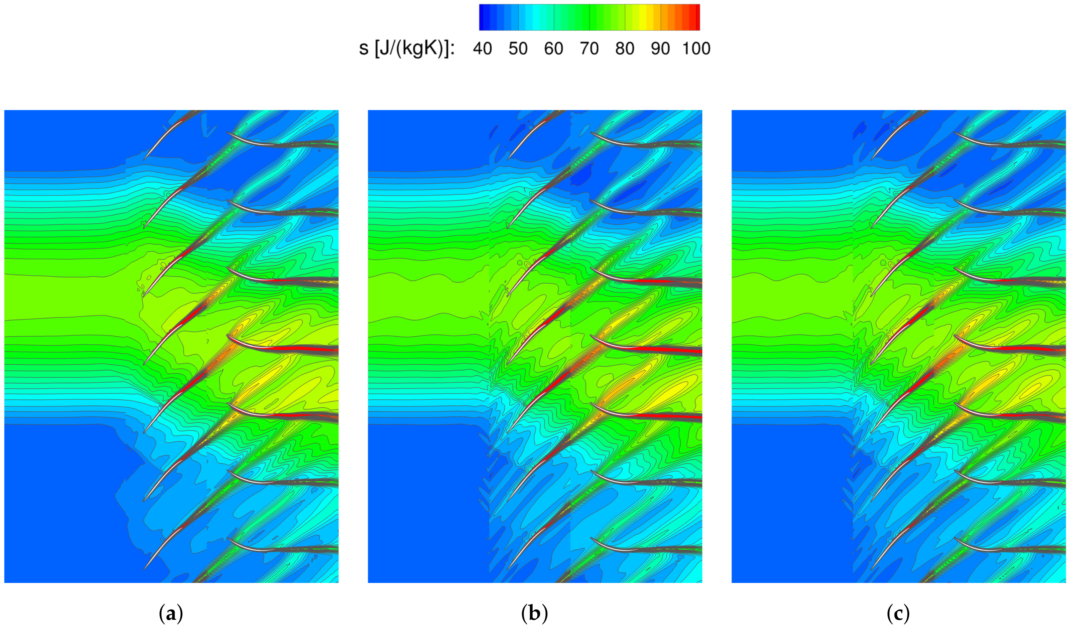
In order to assess the capability of the HB method to predict local flow phenomena, the specific entropy distributions are compared in a blade-to-blade cut at
relative radial height.
Figure 7 depicts the part of the slice in which the ingested boundary layer interacts with the fan stage. The distorted inflow appears in the form of increased entropy levels and is deflected in the direction of rotation of the rotor. Furthermore, the increased profile loading in both rotor and stator results in an increased entropy production in the profile boundary layers during the interaction with the distorted inflow. This results in thicker and more intense entropy wakes. These phenomena are correctly reproduced by the HB simulations.
The fact that the single stator passage HB simulation does not take into account the impact of the indexing on the unsteady part of the flow in the stator can be seen by comparing
Figure 7b,c. There are small differences in the rotor wakes in the middle of the inflow distortion. While in the full annulus simulations (unsteady and HB) the local reduction in axial velocity results in shorter distances between the wakes, this effect is missing in the harmonic balance simulation with a single passage stator.


