Article

Parameterised Model of 2D Combustor Exit Flow Conditions for High-Pressure Turbine Simulations †

by
Marius Schneider
1,*,
Heinz-Peter Schiffer
1 and
Knut Lehmann
2
1
Institute of Gas Turbines and Aerospace Propulsion, Technische Universität Darmstadt, Otto-Berndt-Straße 2, 64287 Darmstadt, Germany
2
Turbine Aerodynamics and Cooling, Rolls-Royce Deutschland Ltd. & Co. KG, 15827 Blankenfelde-Mahlow, Germany
*
Author to whom correspondence should be addressed.
This paper is an extended version of our paper published in European Turbomachinery Conference ETC12, 2017, Paper No. 24.
Int. J. Turbomach. Propuls. Power 2017, 2(4), 20; https://doi.org/10.3390/ijtpp2040020
Submission received: 8 August 2017 / Revised: 3 November 2017 / Accepted: 4 December 2017 / Published: 8 December 2017

Abstract

:
An algorithm is presented generating a complete set of inlet boundary conditions for Reynolds-averaged Navier–Stokes computational fluid dynamics (RANS CFD) of high-pressure turbines to investigate their interaction with lean and rich burn combustors. The method shall contribute to understanding the sensitivities of turbine aerothermal performance in a systematic approach. The boundary conditions are based on a set of input parameters controlling velocity, temperature, and turbulence fields. All other quantities are derived from operating conditions and additional modelling assumptions. The algorithm is coupled with a CFD solver by applying the generated profiles as inlet boundary conditions. The successive steps to derive consistent flow profiles are described and results are validated against flow fields extracted from combustor CFD.

1. Introduction

1.1. Background

Advances in the reduction of emissions have led to the development of novel combustor technologies that impact the turbine design, usually referred to as combustor–turbine interaction (CTI). The influence is mainly downstream in the form of swirl, hot streaks, and elevated turbulence levels approaching the high-pressure turbine (HPT) but there is also an upstream effect of the nozzle guide vane’s (NGV’s) potential field which is noticeable one axial chord-length upstream of the NGV, as reported by Klapdor [1].
The phenomena are investigated experimentally in turbine rigs with so-called combustor simulators (Chana et al. [2], Povey et al. [3], Krichbaum et al. [4]). Flow field measurements behind a real combustor in the presence of NGVs are reported by Cha et al. [5]. The main drawback of these rigs is the missing chemical reaction within the combustor which can prevent the formation of precessing vortex cores and lead to different swirl flow modes according to Hall et al. [6]. The typical numerical approach is to run two separate Reynolds-averaged Navier–Stokes (RANS) simulations of the combustor and turbine, and to exchange flow conditions at a defined interface (referred to as combustor turbine interface), i.e., combustor outlet conditions are used as turbine inlet conditions. Novel approaches make use of unsteady, time step-wise coupling of the combustor and turbine codes (Vagnoli et al. [7]) or aim towards an integrated simulation of combustor and turbine together with RANS as done by Klapdor [1], Raynaud et al. [8], or by using large eddy simulations (LES) as per Koupper et al. [9]. Turbine designers are interested in how the approaching flow field affects the HPT’s aerodynamics and cooling performance. Fundamental theories regarding hot streak migration are based on the work of (a) Munk and Prim [10] and (b) Kerrebrock and Mikolajczak [11]. They showed that: (a) in steady flows with constant entropy along each streamline the streamline pattern is not affected by variations of inlet total temperature for an unchanged total pressure distribution; and that (b) hot gas migration through an NGV passage will result in the formation of positive jets in the rotor, i.e., hot gas will preferably accumulate at the blade’s pressure side (PS), also known as preferential heating. According to Ong et al. [12] this will cause additional vorticity at the rotor PS as can be seen in Hawthorne’s vorticity transport equation. The consequence is that inlet swirl mainly affects NGV aerodynamics, whereas hot streak migration is mostly responsible for effects in the rotor. This emphasises the limits of steady numerical analyses of turbines when investigating unsteady rotor–stator interaction in the presence of temperature non-uniformities. Tallman [13] investigated a significant difference in the outlet temperature profiles between steady and unsteady multi-stage simulations.
Different authors have studied the isolated effects of inlet swirl (Giller et al. [14], Qureshi et al. [15], Schmid et al. [16], Beard et al. [17], Insinna et al. [18], and Jacobi et al. [19]), hot streaks (He et al. [20], Basol et al. [21], and Beard et al. [22]) and elevated turbulence (van Fossen et al. [23]). However, there are few data, and no unifying theory exists with respect to their combined effects. Khanal et al. [24] investigated hot streak migration in an NGV passage under swirl and found that the isolated effects on heat load may not be superimposed.

1.2. Scope and Content of This Paper

The combustor turbine interface conditions are of major relevance in the development process as they represent the most important information exchanged between combustion and turbine engineers. However, there is relatively little knowledge published about the impact of realistic interface flow fields on the HPT. The method presented in this paper aims to contribute to the understanding of the downstream effects of the combustor turbine interface conditions by not regarding them as a unique, static boundary condition. Instead, scatter of the flow at the interface, i.e., variations between the different sectors along the circumference or variations of a traverse within the uncertainty band of its prediction, shall be accounted for as well. This is rarely systematically investigated because changes in the interface conditions typically emerge, almost randomly, from changes in the combustor geometry or operation. These are then difficult to separate in order to explain the observed phenomena in the HPT, such as hot streak migration and interaction of inlet swirl with cooling films. The only variation which can be easily studied is the relative clocking of combustor to NGV domain, i.e., a constant circumferential shift of all flow quantities. Analysing shifts of the flow features in the traverse relative to each other is a more challenging task but of great importance, as these determine the downstream trajectory of hot gas and thus the vane and end wall heat load.
Therefore, a method was developed to create a flexible, realistic and physically consistent two-dimensional (2D) flowfield as can be expected at the combustor exit. It is derived from a set of modelling parameters. The aim is to gain full control of the distributions of all flow quantities. The automated generation of boundary conditions (BCs) shall enlarge variability of inflow conditions for turbine simulations and reduce turnaround times.
In the first part, a detailed description of the parameterisation is given. Then, the method is validated against the computational fluid dynamics (CFD) of a rich burn combustor.

2. Method

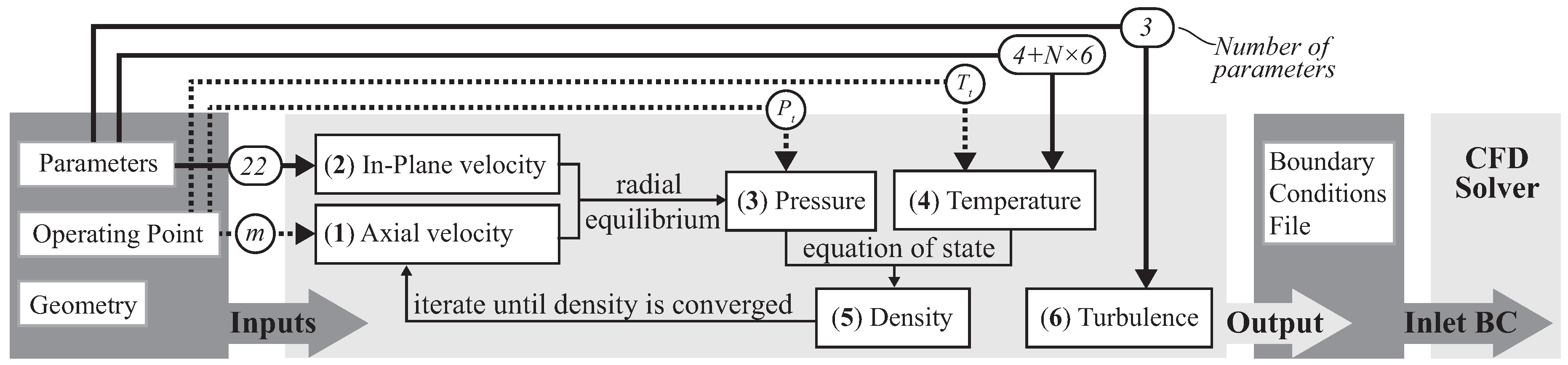
2.1. Overall Parameterisation Strategy

The algorithm described in the following is implemented in a MATLAB tool and coupled with the commercial solver ANSYS CFX [25] for high-pressure turbine CFD by exchanging a boundary conditions file. Inputs to the algorithm are the interface geometry, a set of parameters for the distribution of the flow quantities, and an operating point which is defined in terms of
mass flow m ˙ : = ρ V ax d A = m ˙ DP ,
inlet mean total temperature T ¯ t : = 1 / m ˙ T t d m ˙ = T t , DP ,
inlet mean total pressure p ¯ t : = 1 / m ˙ p t d m ˙ = p t , DP .
The definition of operating conditions is important when it comes to the comparison of the effects of inlet profiles on a turbine. Note that (a) mean quantities are mass-flow averaged, which may lead to difficulties discussed later, and (b) Equation (2) does not fix the flow of energy to the turbine if m ˙ = m ˙ DP is fixed and c p varies with temperature. That is, in general it is not possible to make a turbine with arbitrary 2D inlet conditions always operate at the same mean inlet temperature and energy inflow. Hence, from a point of view considering the combustor and turbine as a coupled system it may be more appropriate to fix H ˙ t : = c p ( T ) T t d m ˙ = H ˙ t , DP instead. The energy input to the combustor (and thus to the turbine) is then equal among different traverses but distributed differently at the combustor turbine interface. However, if losses in the turbine due to secondary flows from different inlet traverses are evaluated based on turbine efficiency, it is more convenient to fix T ¯ t = T t , DP . Otherwise, changes in efficiency caused by additional losses cannot be distinguished from those caused by a shift in operating conditions of the turbine.
The flow quantities at the interface are divided into parameterised quantities of total temperature, in-plane velocity components, and turbulence that are defined from the input parameters and the derived quantities of axial velocity, pressure, and density that must be computed in order to create a physically closed solution. The overall procedure of the computation consists of six steps as shown in Figure 1. The density field is initialised as constant at 1 kg/m 3 and iteratively corrected in steps 1–5 until it is converged, i.e., the maximal relative difference between the old and new density field is less than 0.1%. All flow quantities are subject to the numerical constraint of circumferential periodicity which is commonly used in turbomachinery CFD, allowing for single-passage simulations. It is recognised that due to sector-to-sector variability of the flow fields in a real turbine there may be a considerable influence of one sector on the neighbouring sectors. The presented method can be extended in order to investigate these effects by creating a multi-passage BC enforcing periodicity only at the outermost boundaries and allowing for different non-periodic sectors “inside” the modelled field. An approach for extension is not covered in this paper but can be easily derived for most elements of the algorithm.
The parameterisation of the respective flow fields according to Figure 1 is described in the following paragraphs. In principle the method is equally applicable to rich and lean burn combustors, whereas a minimum amount of inlet swirl is presumed. In total, the parameterisation consists of at least 35 parameters.

2.2. Axial Velocity

The axial velocity component V ax ( r , θ ) has a special role among the field quantities because: (a) it may not be derived from the other flow quantities in the traverse in closed form and thus in principle can be set arbitrarily, i.e., without any physical restrictions, in the parameterisation process as long as Equation (1) is fulfilled; and (b) it may not be prescribed explicitly as an inlet boundary condition for HPT simulation if total quantities are imposed. Typically, an inlet boundary condition for compressible turbomachinery CFD consists of total pressure and temperature, flow angles, and turbulent quantities (note the difference between imposing flow angles and velocitiy components). The velocity magnitude at turbine inlet is therefore not fixed by the inlet condition and may freely converge to a stable state in the solution process of CFD. This distribution V ax ( r , θ ) is unknown in the parameterisation process, before a simulation is run.
It is therefore not reasonable to distribute V ax ( r , θ ) based on a set of arbitrary parameters like the other parameterised quantities in the algorithm because this distribution cannot be transferred to the flow solver as a BC, and thus it will most likely converge to a different distribution nonetheless. Still, it is desirable to estimate V ax ( r , θ ) in the parameterised model as close as possible to the converged CFD solution for the following reasons: V ax ( r , θ ) determines (a) flow angles, (b) kinetic energy and dynamic pressure, and (c) the distribution of mass flux d m ˙ ( r , θ ) at the turbine inlet and thus influences the mass flow averaging in Equations (2) and (3). That is, the operating conditions set in Equations (2) and (3) will be reproduced in CFD only if the assumed distribution for V ax ( r , θ ) in the model exactly matches the converged CFD.
However, there is no generally valid model to derive axial velocity from the known field quantities, i.e., a general functional relation V ax ( r , θ ) = f ( V r ( r , θ ) , V t ( r , θ ) , p t ( r , θ ) , ρ ( r , θ ) , ) is unknown. Estimations of V ax ( r , θ ) can therefore be drawn only empirically from existing data which does not form part of the presented model and remains an open task for future improvement of the method. In the results shown in this paper, axial velocity is specified in the most simple approach, which is a constant distribution V ax = c o n s t . , in order to display the worst case results if no information on V ax ( r , θ ) is available a priori.

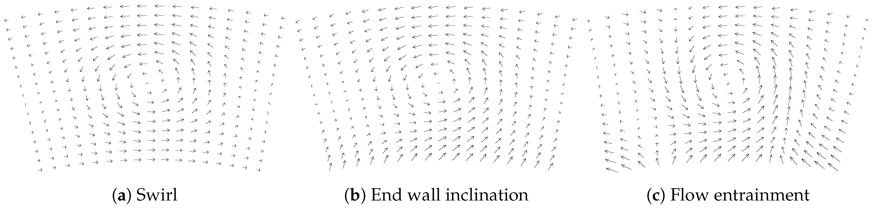
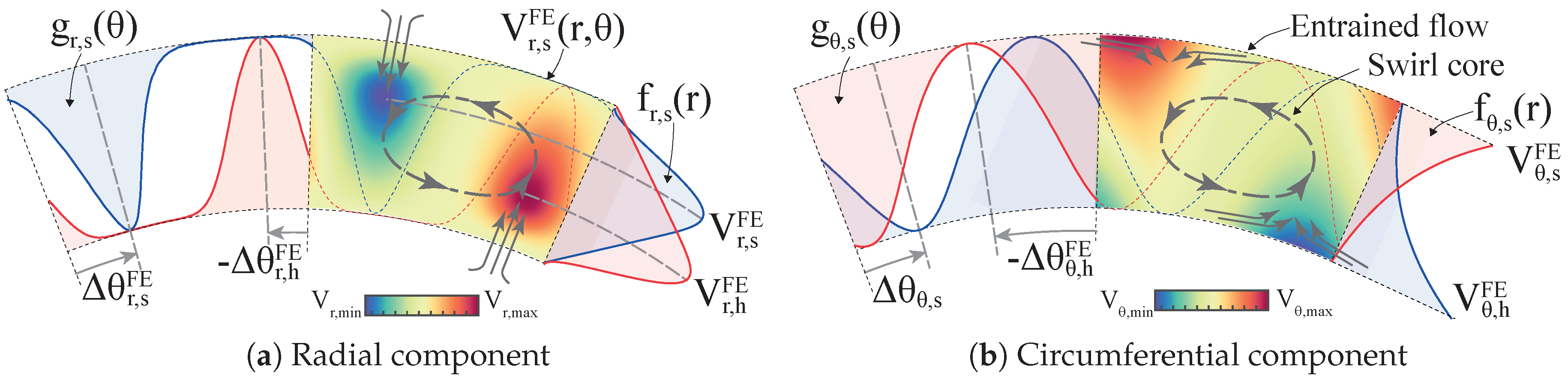
2.3. In-Plane Velocity Field

The in-plane velocity fields, i.e., V r ( r , θ ) and V θ ( r , θ ) , are superimposed from three components which are all forced to be circumferentially periodic and then combined to the final flow field (Figure 2c). The components account for combustor swirl, cross flow components from the inclination of the end walls, and flow entrainment due to swirl, and will be described in the following.

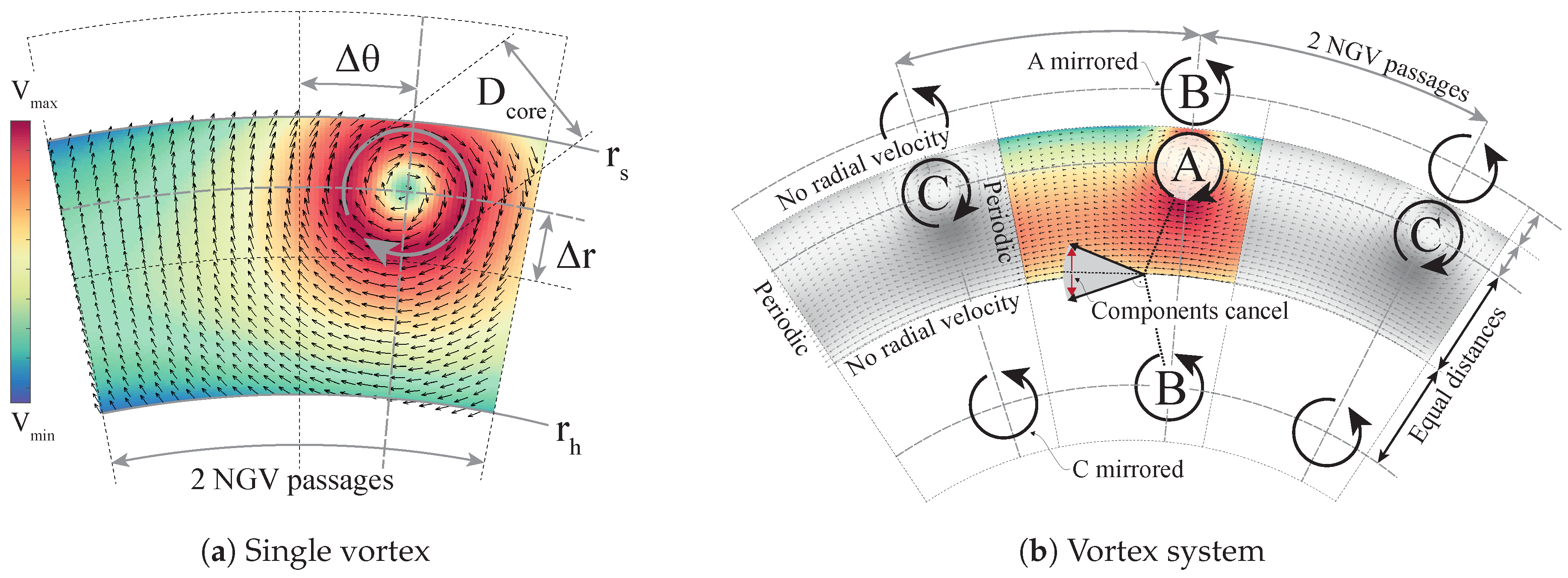
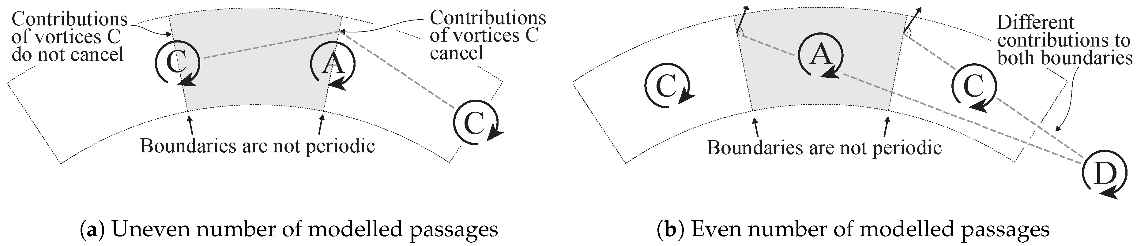
2.3.1. Swirl Velocity Field

It is assumed that a single swirl core is located in each passage, although the method is expandable to multiple swirl cores per passage. For the parameterisation of the swirl velocity field a fixed swirler-to-vane count (1:2 in the data shown) is assumed. The swirl component V S ( r , θ ) is defined relative to a position which is offset from the centre of the sector by Δ r S and Δ θ S (Figure 3a). It is calculated using an empirical vortex model. In the data shown in this paper, a time-independent Lamb–Oseen type of vortex
V S ( R ) = d S Γ 2 π R 1 exp 4 R 2 ( D core S ) 2
is used, which offers three parameters; the swirl direction d S = ± 1 , the diameter of the viscous swirl core D core S , and the swirling strength determined by Γ which, according to Gupta [26], is accounted for in non-dimensional form by the swirl number
S = ρ V ax V S R 2 d R ( r s r h ) ρ V ax 2 R d R .
The parameters used for modelling the 2D swirl field are displayed in Figure 3a. However, it can be seen that the modelling of a single vortex does not yield a suitable inlet boundary condition for flow angles because the left and right side of the sector are not periodic and there are flow vectors pointing outwards at the hub and shroud end wall. A simulation using the displayed vectors as inlet boundary condition would thus very likely diverge. In order to adapt the swirl field to the requirements of CFD, additional elements are used in the model. Establishing a flow with no streamlines penetrating the hub and shroud wall, i.e., V r ( r h / s ) = 0 , can be achieved by placing two virtual, mirrored vortices of equal strength and wall distance as the vortex in Figure 3a outside the modelled flow sector at θ m S = θ S and r m S = r h / s + ( r h / s r S ) with reversed swirl direction d m S = d S . These are labelled Ⓑ in Figure 3b. It can be seen that the radial flow component induced at the hub and shroud from vortex Ⓐ is thus cancelled by the contributions from vortices Ⓑ.
The maximal deviation from 0 of the radial angle at the hub, introduced by the hub curvature, behaves as max [ α r ( r = r h ) ] max [ α r ] 0.08 ( r h r s r h ) 0.8 + 0.024 for S = 0.2 and 16 sectors. That is, for r h r s r h > 1 the maximal deviation is less than 2 (10% of the maximal pitch angle) and for r h r s r h > 4 , which is at the order of realistic geometries, the deviation is less than 1 (5% of the maximal pitch angle).
In order to make the boundaries at the sides of Figure 3a periodic, the influence of the neighbouring passages must be accounted for. The respective vortices are labelled Ⓒ in Figure 3b. For reasons of symmetry, however, the modelling of three passages is not sufficient to establish periodic boundaries for an arbitrary clocking position of the vortices relative to the sector. In fact, the full annulus must be modelled since a smaller number of passages will lead to unequal sector boundaries on the left and on the right at certain clocking positions of the vortex. This is illustrated in Figure 4 for an uneven number of modelled passages clocked half a pitch and for an even number of passages clocked to the centre. In both cases the resulting flow field in the grey passage is non-periodic.
In order to overcome this problem all vortices Ⓐ around the circumference are modelled, including their respective mirrored counterparts Ⓑ, and the influence of all of these vortices on the modelled passage is superimposed. For the sector geometry shown this results in a total of 48 modelled vortices (16 sectors × 3 vortices). The result of this procedure is an arbitrarily positionable vortex creating a velocity field that is always periodically repeatable and has approximately zero radial velocity at the hub and shroud (Figure 5a).
The shape of the modelled vortex has a strong influence on the inlet pressure profile and the stability of the vortex, i.e., the axial position of its breakdown. Axisymmetric vortices as shown in Figure 5a tend to be more stable than non-axisymmetric ones, which can be observed in the realistic combustor turbine interfaces of some combustor designs.
In order to resolve this effect, an additional parameter θ SCL S is introduced to “stretch” the vortex in circumferential direction. This is done by superimposing the flow fields of multiple vortices along the circumference as indicated in Figure 5b. The parameter is referenced to one pitch of the flow field, i.e., θ SCL S = 0 corresponds to an axisymmetric vortex and θ SCL S = 1 to a vortex stretched along the circumference of an entire passage. The stretching is similarly applied to all mirrored Ⓑ and neighbouring Ⓒ vortices along the circumference. Note that the superposition and vortex stretching processes interfere with the originally prescribed value of S for axisymmetric swirl making it a pseudo-swirl number.

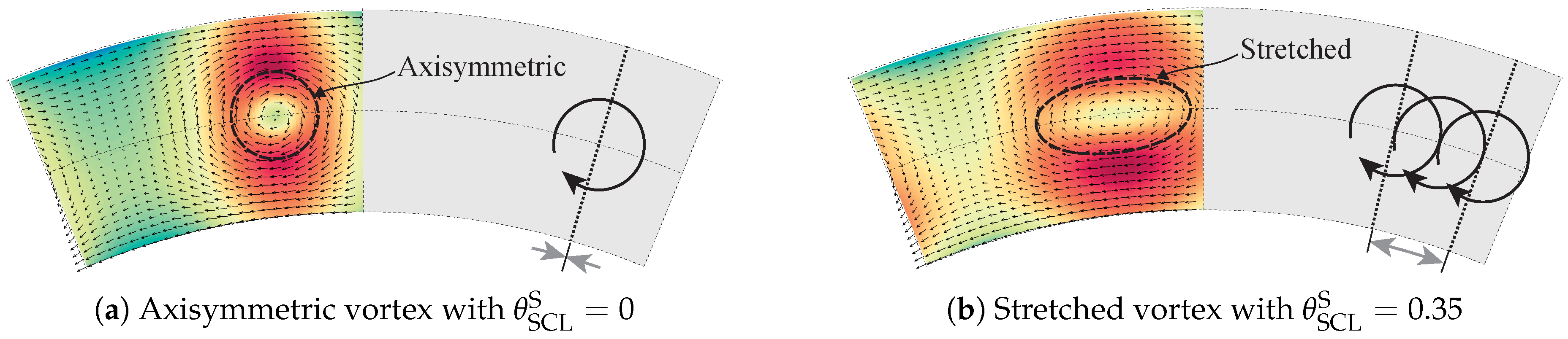
2.3.2. End Wall Inclination

In the modelling of the swirling flow described in the previous section, the flow at the end walls is forced to have zero radial velocity at the hub and shroud walls to prevent vectors going out of the flow domain. Due to the convergence of the annulus between the combustor and NGV, the endwalls are typically inclined at the combustor–turbine interface, imposing a finite radial inward-bound flow component. Therefore, an additional flow field with radial component specified by V r , h / s E = V r ( r h / s ) is added to the flow vectors close to the hub and shroud to account for local endwall inclination as shown in Figure 2b. The component is uniform in circumferential direction in order not to affect the periodicity of the swirl field. The imposed radial component decays exponentially in the radial direction in order to influence only the flow close to the end walls and prevent interference with the previously created swirl field.

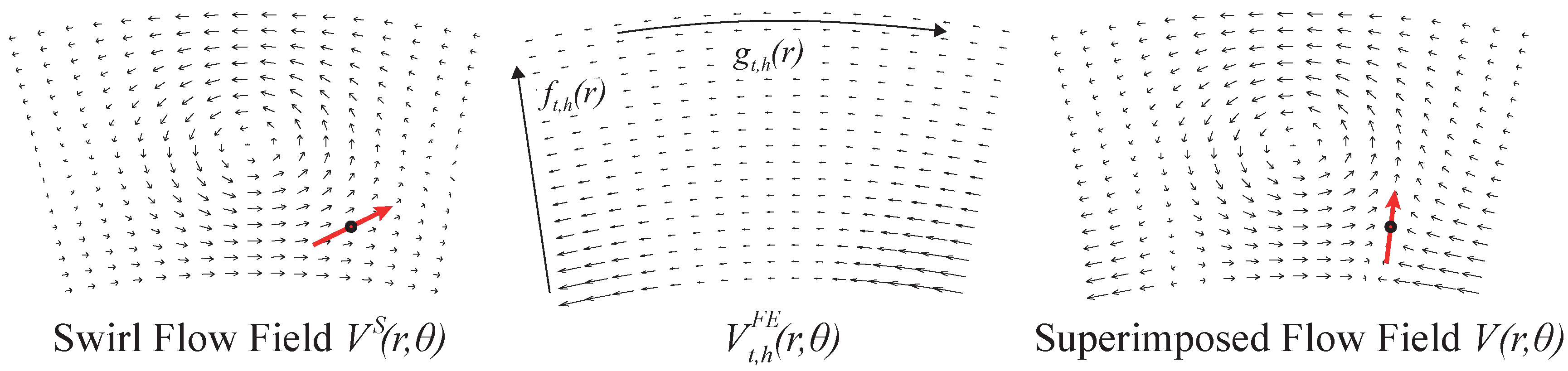
2.3.3. Flow Entrainment

The approach described above does not suffice to generate realistic combustor exit swirl fields because flow in the hub and shroud end wall regions tends to be locally entrained by the overall swirling motion. This imposes additional, two-dimensional flow components which are not represented by vortices as shown in Figure 5 and must be accounted for separately. The modelling of these components relies on empirically determined functions which may be adjusted by 14 different parameters, allowing for clocking and change in shape of the profiles. Details of the parameterisation are shown in Appendix A. A typical cross flow field resulting from this procedure is displayed in Figure 2c.

2.4. Pressure

The pressure profile may not be specified independently by parameters because it must satisfy the parameterised velocity field. In order to grant stability, the assumption of radial equilibrium is used to derive the pressure field, i.e., the pressure gradient is distributed so that it balances the accelerations resulting from the velocity field. Viscous effects, time dependency, and derivatives in axial direction are neglected. The pressure gradient can then be computed on lines of constant θ from
p r = ρ V r V r r + 1 r V θ V r θ V θ 2
where V r , V θ , and ρ are known quantities. With the pressure gradient known at every position of the sector, the hub pressure p h = p ( r h ) must be specified in order to fix the pressure field. The pressure at every grid node can then be computed by marching in radial direction on each layer p ( r ) = p ( r Δ r ) + Δ p Δ r . The hub pressure p h on each layer of constant θ is iteratively adjusted so that Equation (3) for the averaged inlet total pressure p ¯ t is fulfilled.

2.5. Temperature

The 2D total temperature profile is parameterised independently of the velocity field. It is assumed to consist of a circumferentially uniform baseline profile which accounts for the temperature boundary layers (Figure 6a) and an arbitrary number of hot spots (Figure 6b) referenced by index i [ 1 , , N ] , creating non-uniformities in the circumferential direction. The baseline profile is used to adjust the overall temperature level to match the operating point and to enforce a temperature drop towards the end walls.

2.5.1. Baseline Profile
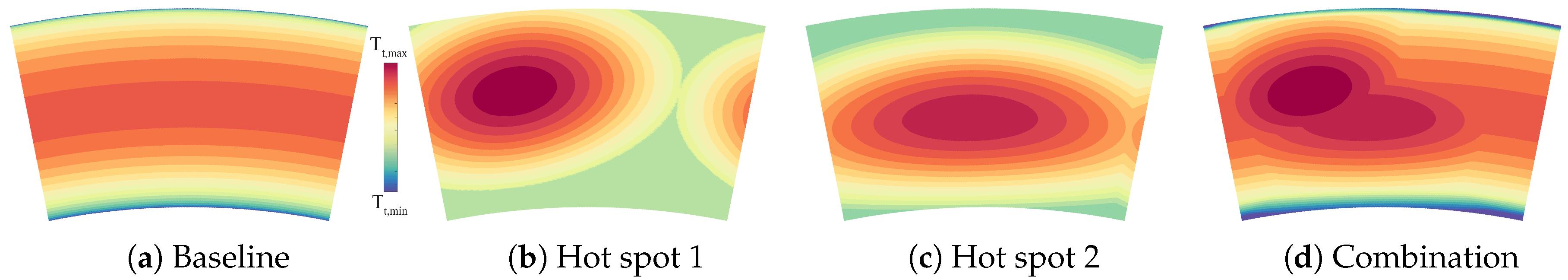
The radial shape of the baseline profile is defined by the power function T BSL ( r ) = ( r r h + r s 2 ) ϕ with the exponents ϕ = 2 T h / s BSL accounting for temperature boundary layers resulting from hub and shroud end wall cooling. The profile is linearly scaled so that its minimal and maximal temperatures are at T min , h / s and T max BSL , respectively, as shown in Figure 6.

2.5.2. Hot Spots

Each hot spot i is modelled as a 2D Gaussian distribution which can be approximated by T i ( r , θ ) = T max i exp a i ( Δ θ i ) 2 + 2 b i ( Δ θ i ) ( Δ r i ) c i ( Δ r i ) 2 with the coefficients a i = cos ( ϕ i ) 2 2 ( σ x i ) 2 + sin ( ϕ i ) 2 2 ( σ y i ) 2 , b i = sin ( 2 ϕ i ) 4 ( σ x i ) 2 + sin ( 2 ϕ i ) 4 ( σ y i ) 2 and c i = sin ( ϕ i ) 2 2 ( σ x i ) 2 + cos ( ϕ i ) 2 2 ( σ y i ) 2 . Each spot i is centred at a position offset from the centre of the sector by Δ r i and Δ θ i and has an individual peak temperature T max i , scaling parameters σ x i , σ y i , and rotation angle ϕ i . The implication of the individual parameters is displayed in Figure 6b.

2.5.3. Overall Profile

The overall stagnation temperature profile is derived by superimposing the maximum of the N hot spots and the baseline profile at each point outside of the temperature boundary layer T ( r , θ ) = max T 1 ( r , θ ) , , T N ( r , θ ) , T BSL ( r ) as shown in Figure 7.
The maximum temperature of the baseline profile T max BSL is not a free parameter but it is used to iteratively adjust the inlet temperature so that the operating point (Equation (2)) is matched.

2.6. Turbulence

Turbulent fluctuations at the combustor turbine interface are not connected to the time-averaged flow by any physical conservation laws but rather depend on the history of the flow before that interface. In the model, the distribution of turbulent quantities is therefore entirely determined by heuristic correlations for turbulence intensity T u , and length scale L which are assumed to be proportional to the local shear strain rate of the previously created velocity field with a blending towards the end walls. These can be converted to any two quantities needed for two-equation model boundary conditions. Three parameters for mean intensity T u ¯ , maximum length scale L max , and a scaling factor T u SCL controlling homogeneity are open in the model.
As an alternative, more complex modelling approach turbulent quantities can be represented by superimposing a baseline profile with turbulent spots, similar to the previously described parameterisation of temperature at the cost of a strongly increased parameter count.

3. Validation

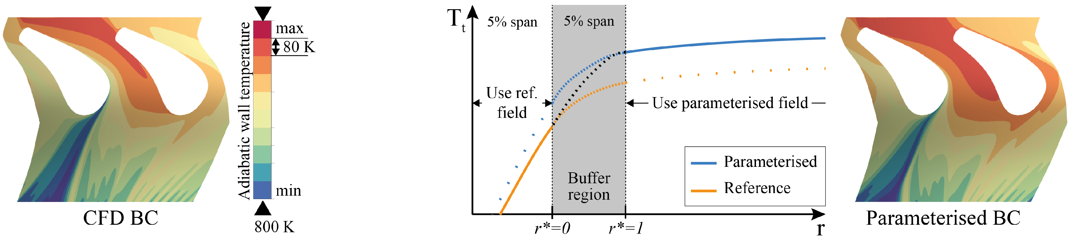
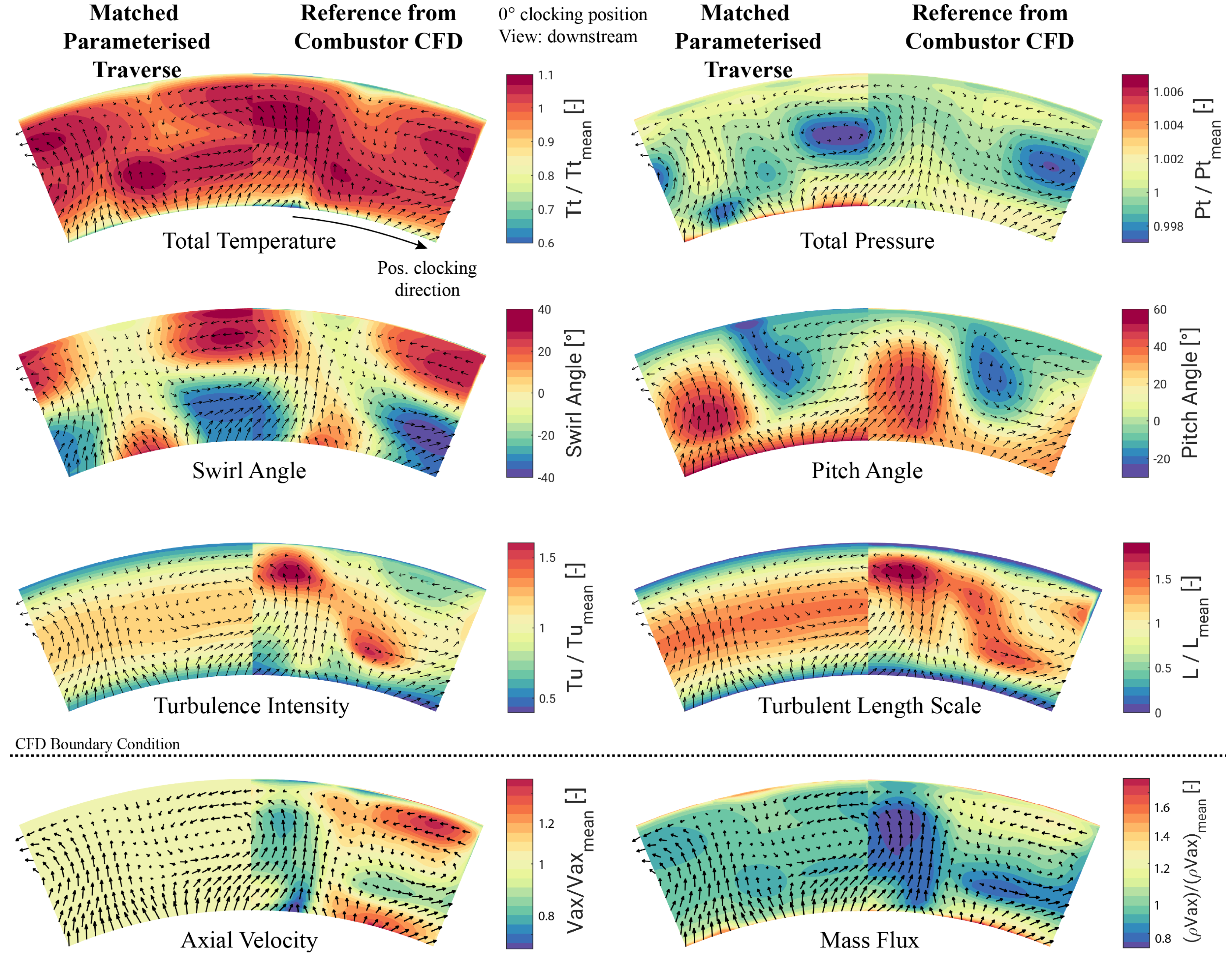
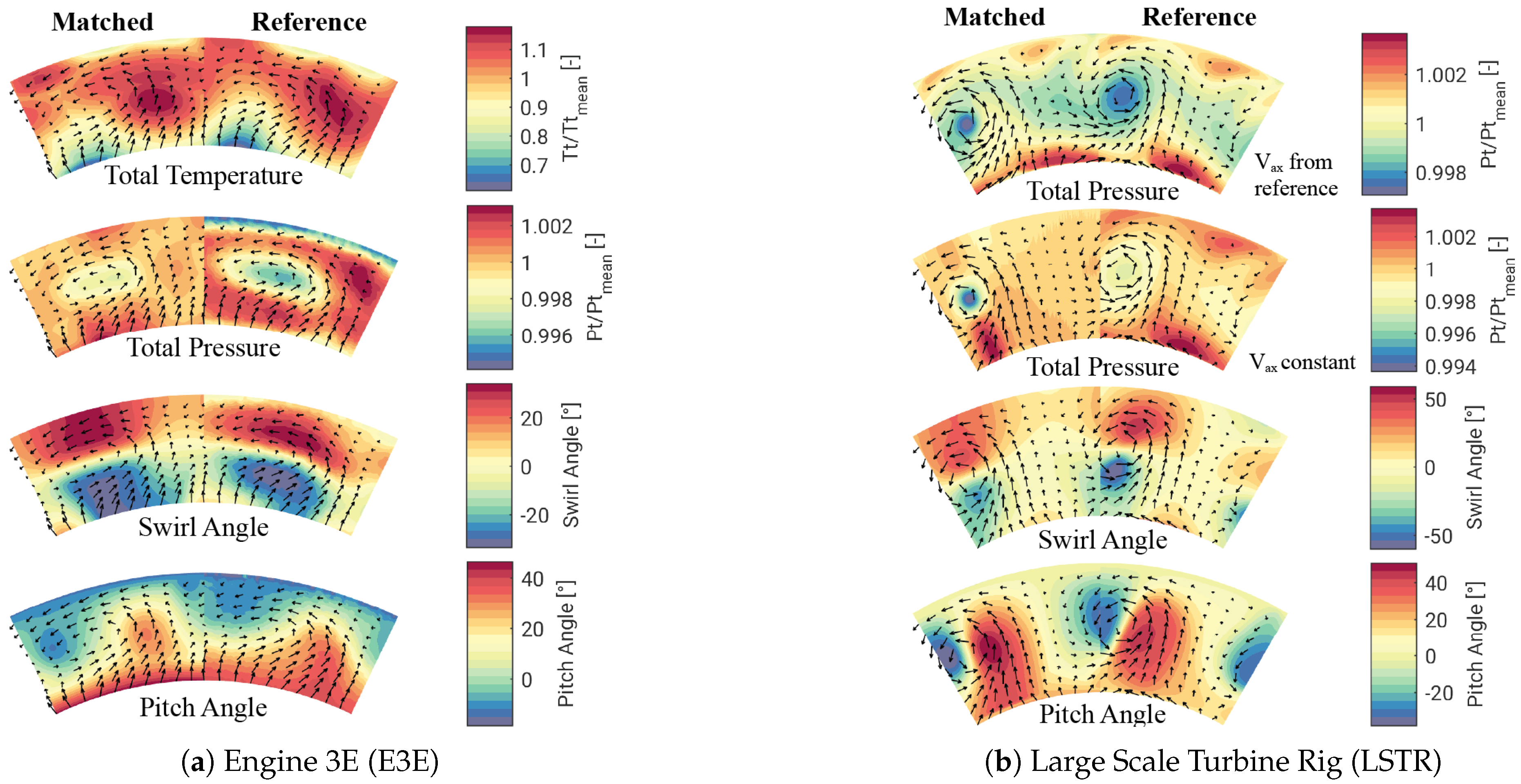
3.1. Matching a Target Interface
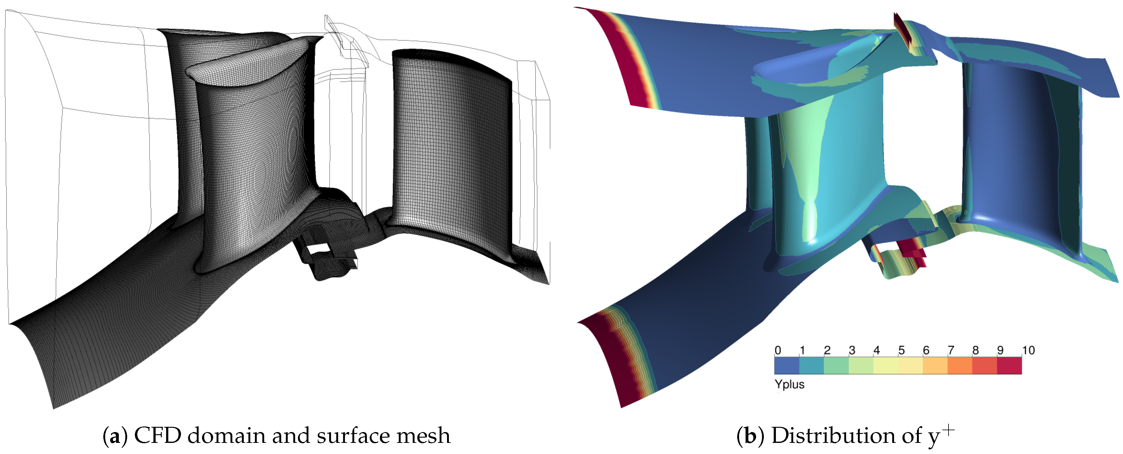
In order to evaluate the capability of the parameterised traverses to reproduce boundary conditions from combustor CFD, both are applied to the same CFD set-up of an HPT. Stage efficiency and the distribution of wall temperature and Nusselt number serve as criteria for the validation. The simulations use the mixing plane approach; the focus is therefore on the reproduction of the flow within the NGV passage. In order to allow the assessment of the generality of the method, matches to a number of additional traverses are shown in Appendix B.
The parameter set that represents best the reference flow interface is determined by a numerical optimisation algorithm. For the presented approach the genetic optimiser implemented in MATLAB [27] was used. In order to minimise computation time, parameter limits were set to an ϵ -environment about a starting point. The start values were determined by iterative manual adjustment of the model parameters based on the plots shown in Figure 8. The single objective fitness function to be minimised is
y = k = 1 K C k θ = θ min θ max r = r min r max ( Δ Φ k ( r , θ ) ) 2 ξ θ = θ min θ max r = r min r max ξ 1
where K is the number of field quantities to be simultaneously optimised, C k is a weighting factor, Δ Φ k ( r , θ ) = Φ k ( r , θ ) Φ k ref ( r , θ ) max [ Φ k ref ( r , θ ) ] is the normalised difference to the reference solution of quantity Φ k at each node of the interface, and ξ determines the averaging procedure. The optimisation was iterated with a population size of 200 until the average relative change of the best individuals in the last 50 generations remained within the convergence limit of 1%. It was run independently for: (a) the temperature field with K = 1 , C = 1 , Φ = T t , ξ = 1 ; and (b) pressure and flow angle distributions with K = 3 , C = [ 0.5 , 0.25 , 0.25 ] , Φ = [ P t , α θ , α r ] , ξ = 1 . A grid-independent creation of traverses was achieved on [ r × θ ] = [ 200 × 200 ] nodes. Grid independency was assumed when maximal changes in total pressure due to grid refinement were below 100 Pa. The temperature was modelled by N = 3 hot spots, i.e., 47 parameters were fitted in total for all six fields. The number of hot spots needed was estimated based on the features of the target traverse and confirmed a posteriori by the results shown in Figure 12.
In Figure 8, the inlet boundary conditions for turbine CFD resulting from a RANS simulation of a modern rich burn combustor with inlet swirl are compared with the parameterised version of the interface resulting from the optimisation. Distribution of stagnation temperature, pressure, and flow angles agree well with the target traverse. As described above, the intensity and length scale of the turbulent fluctuations are derived from heuristic correlations and are controlled only by three parameters. This is why in Figure 8 the turbulent quantities agree only in terms of the mean levels. The implications of this discrepancy are discussed in Appendix C.
Distributions of axial velocity V ax ( r , θ ) and mass flux ρ ( r , θ ) V ax ( r , θ ) are also plotted in Figure 8 for completion. These fields are not specified as CFD inlet BC. Both fields show a large blockage zone in the left part of the reference sector and a zone of acceleration close to the end walls of the right half. The blockage is assumed to result from the hub flow entrainment visible in the distribution of pitch angle. The acceleration outside the blockage zone is assumed to result mainly from the distribution of total pressure. An acceleration of axial flow in regions of high temperature is not visible, which justifies the decoupling of velocity and temperature parameterisation in this case.
It can be seen that acceleration and blockage of axial flow are not captured by the model since V ax ( r , θ ) = c o n s t . is assumed. In order to account for these effects, the axial velocity profile from the reference case shown in Figure 8 could be readily used instead.

3.2. CFD Setup

The geometry used in the simulations is an engine-representative, single-stage high-pressure turbine with two nozzle vanes and one rotor blade included as shown in Figure 9. Vane and end wall film cooling as well as cooling slots in front of the vanes are not included in the model but sealing and leakage slots upstream of the rotor are resolved.
Rotor and NGV are meshed structured using hexahedra. No non-matching interfaces were used to connect the rotor cavities and main flow domains. The quality of the low-Reynolds mesh is summarised in Table 1. The non-dimensional wall distance y + as shown in Figure 9 is below 2.5 in a large part of the domain. High y + values above 20 could not be avoided at the rotor seal and leakage inlets in order to prevent highly skewed cells. At the main flow inlet, high y + values of about 50 were intentionally set in order to numerically damp the flow in the boundary layer. Previous studies had shown that lower values of y + at the domain inlet in combination with complex 2D BCs caused high residuals in these regions as well as poor convergence of stage efficiency. High values of y + are handled by a blending between wall functions and the low-Reynolds solution in the solver.
Mesh sensitivity was evaluated in a grid refinement study. A coarser mesh with 3.1 million (Mio.) cells (1.8 Mio. in stator, 1.3 Mio. in rotor) and a finer mesh with 12.7 Mio. cells (7.4 Mio. in stator, 5.3 Mio. in rotor) were simulated. Meshes with higher cell counts could not be included into the mesh study due to insufficient convergence.
The NGV wall temperature shows a maximal difference of 2% between the solution on the baseline grid and the fine grid (Figure 10a) and can be regarded as mesh-independent for the purpose of the present study. Differences in the solution on the finest mesh in isentropic efficiency η and NGV pressure loss coefficient C p defined as
η : = j H ˙ t , in , j H ˙ t , out c ¯ p j m ˙ in , j T t , in , j 1 p t , out / p t , in γ ¯ 1 γ ¯ and C p : = p t , in p t , out NGV 1 2 ρ in V in 2
amounted to Δ η = 0.04 % absolute and Δ C p = 3 % relative (Figure 10b). These were regarded as acceptable for comparison in a validation. All flow quantities needed for the computation of η and C p are mass flow-averaged on the respective boundaries and the fluid properties c ¯ p and γ ¯ are averaged between each inlet and the stage outlet.
The solver used for this study is ANSYS CFX v17.0 [25]. The boundary conditions at the main inlet, which is 1.1 axial chord lengths upstream of the NGV, are the modelled 2D quantities shown in Figure 8 at 0% relative clocking position between the BC and NGV domain. A fixed mass flow m ˙ DP is prescribed at the outlet. The simulations assume steady state using a mixing plane between the nozzle and rotor. Turbulence is modelled using the SST-k- ω model by Menter [28] assuming fully turbulent flow. The conservation equations are discretised with averaged blending factors above 0.9. The compressible gas is assumed ideal with a temperature-dependent heat capacity. All simulations are run for 500 iterations with all averaged residuals less than 1 × 10 5 and all imbalances below 0.02% of the corresponding maximum value.

3.3. Results

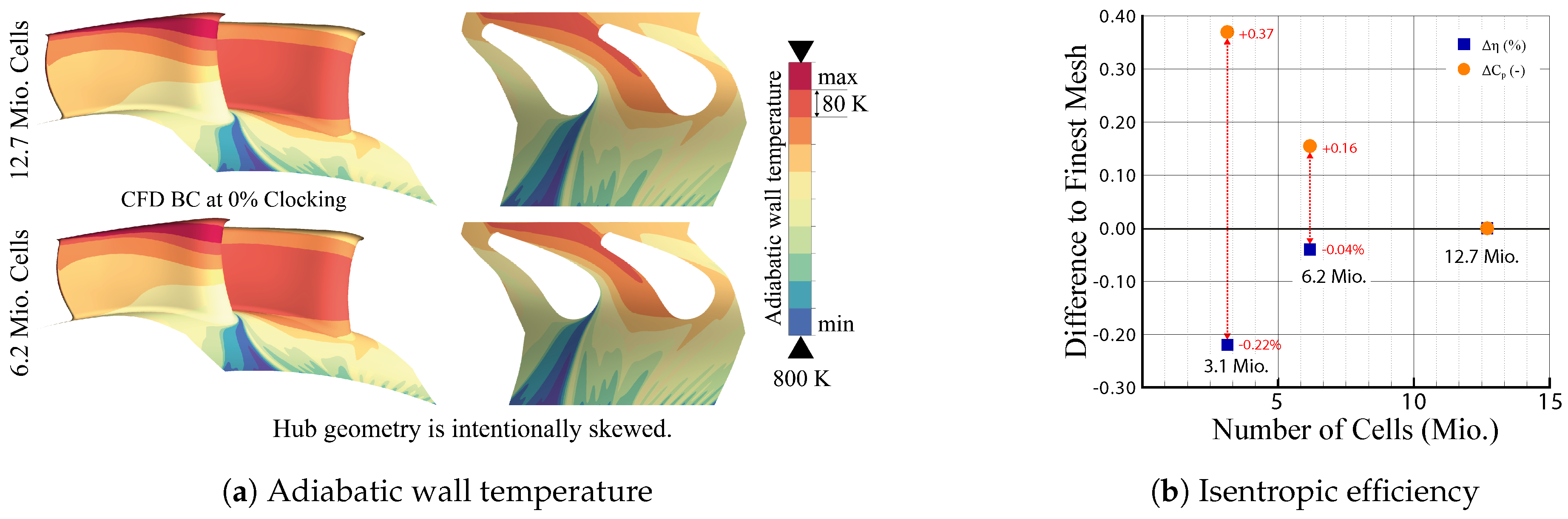
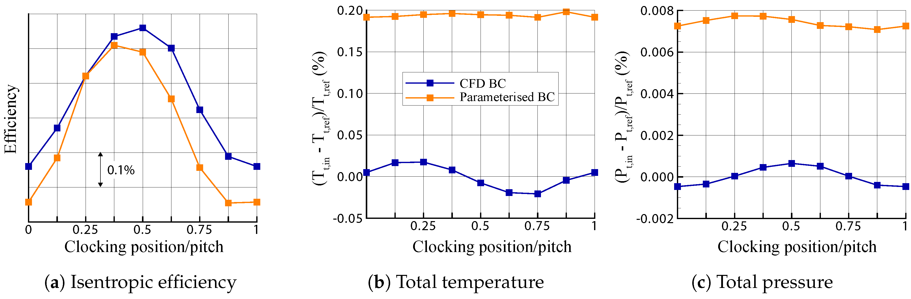
3.3.1. Stage Efficiency

All simulations converged to the same operating point of the turbine: Maximal deviations between the the converged CFD solution and the specified reference conditions are Δ T ¯ t = 0.2 % , Δ p ¯ t = 0.008 % , and Δ m ˙ = 0.005 % . Note that mass flow is prescribed by the outlet boundary condition. Inlet capacity changes were below 0.04% of the maximal value. Isentropic stage efficiency η for inlet profiles from CFD and the parameterisation algorithm is shown in Figure 11 at eight clocking positions of the inlet BC relative to the NGV vanes.
The overall trend and magnitude of η are represented well. Clocking positions of the extrema show an offset of about 1/8 of the sector pitch and the maximal difference at a given clocking position is Δ η = 0.15 % . When analysing the effect of different inlet profiles on stage efficiency it is important to maintain constant operating conditions in order to monitor only efficiency changes due to losses in the flow, not changes in the operating point. In Figure 11b,c deviations of inlet conditions from the reference are displayed. For both the boundary conditions from CFD and the parameterised counterparts, the inlet conditions are sufficiently constant for a comparison of efficiencies.
However, it can be seen that the parameterised traverse operates at a slightly higher inlet temperature and pressure than specified by reference conditions (Equations (2) and (3)). The reason for this is discussed in Section 2.2: The error in the assumption of a constant axial velocity in combination with mass flow averaging leads to a shift in T ¯ t and p ¯ t .

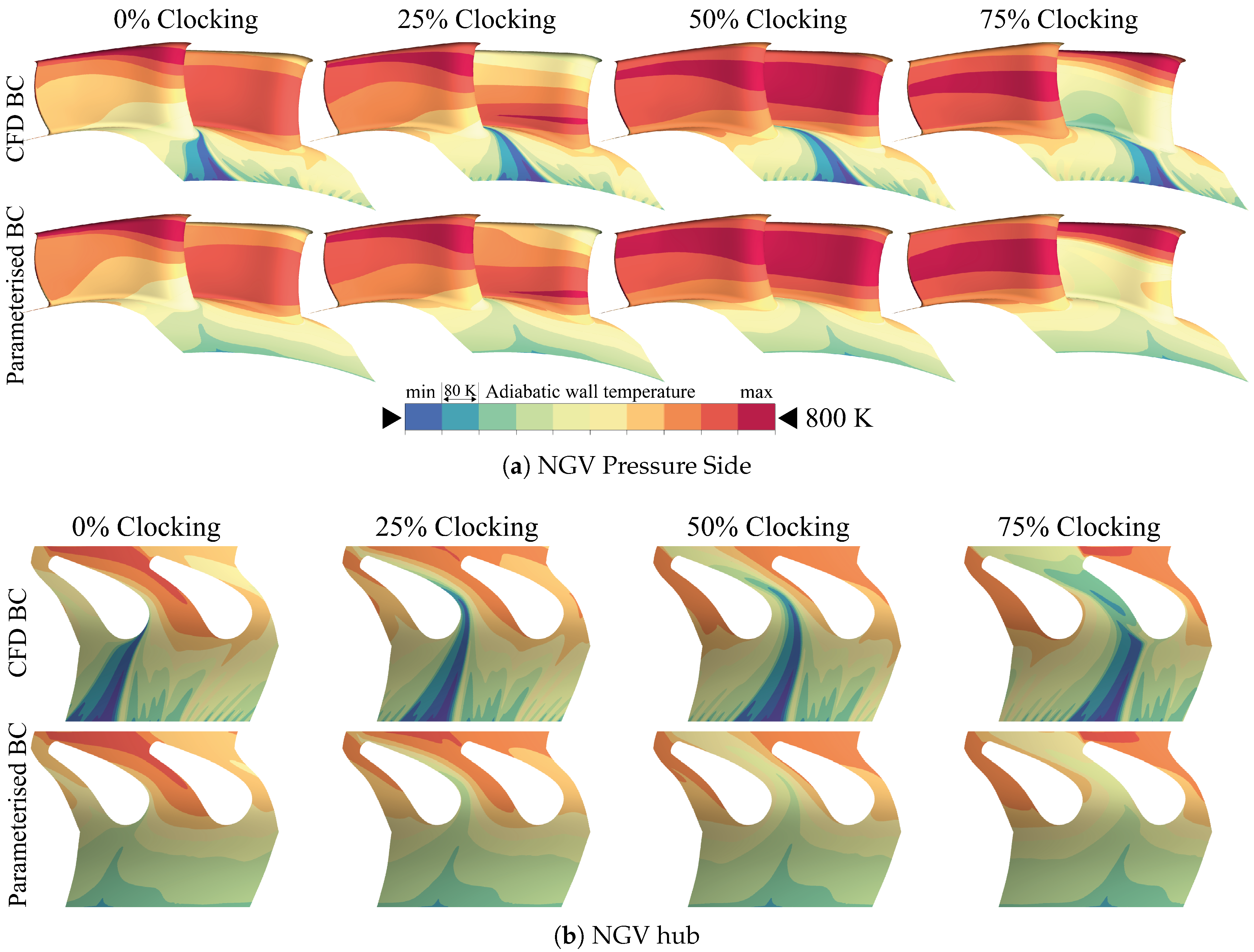
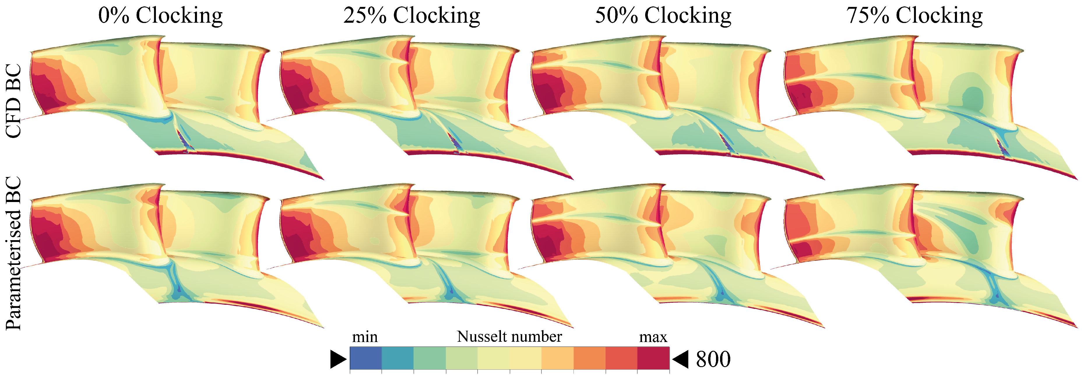
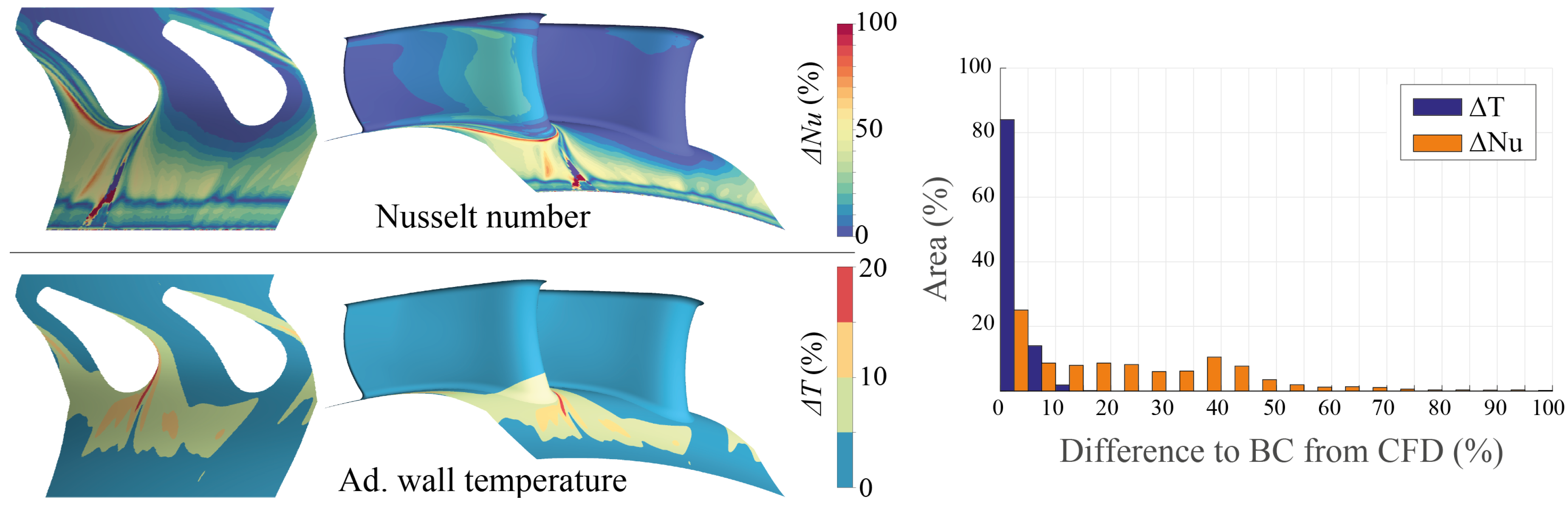
3.3.2. Heat Transfer and Wall Temperatures

In order to evaluate the applicability of the proposed method in thermal analyses, distributions of adiabatic wall temperatures and Nusselt number
N u : = h ad c λ
were compared.
Temperature distributions agree well, especially on the vane surfaces and the rear part of the hub end wall. This indicates that the migration of hot streaks and the secondary flows driving heat transfer can be adequately reproduced. In Figure 12b it can be seen that cold streaks from combustor wall film cooling at the front part of the hub end wall cannot be resolved by the model since the baseline temperature profile is assumed to be circumferentially uniform (Figure 6a). An influence of these coolant streaks on the surface temperatures in the passage can clearly be seen at the 75% clocking position. A parameterised representation of wall film cooling would introduce many additional parameters impeding a practical application of the method. It was therefore refrained from modelling wall film cooling in this paper and the integration of an efficient model remains a task for future work.
An approach to overcoming this problem is use of the reference temperature field close to the end walls and the parameterised temperature field in the main flow region, thus maintaining the flexibility of the parameterised temperature field. A smooth transition can be achieved using a blending of both fields in a buffer region ranging from r * = 0 to r * = 1
T t ( r * , θ ) = r * T t par ( r * = 1 , θ ) + ( 1 r * ) T t ref ( r * = 0 , θ )
as illustrated in Figure 13. It can be seen that the representation of hub wall temperatures is significantly improved by this method.
Distributions of N u are shown in Figure 14. The largest discrepancies can be seen on the pressure side of the right vane at 75% clocking. A minimum in N u on the PS of the left vane cane be observed moving from the PS/shroud corner to midspan from 0% to 75% clocking. The low heat transfer in this region is caused by a counter-rotating vortex pair forming in addition to secondary flows described by classical models. These vortices drive fluid away from the vane surface, thus thickening the boundary layer and decreasing heat transfer locally. They are induced by the low pressure zone at the inlet swirl core that causes the vortices to roll-up at the leading edge as described by Jacobi et al. [19].

4. Conclusions

A method for the parameterised generation of realistic rich and lean burn combustor exit traverses for HPT CFD is described and validated. All flow quantities necessary for consistent RANS CFD boundary conditions are generated in a physically closed, iterative procedure from a set of at least 35 parameters determining velocity, temperature, and turbulence. The pressure profile is not open for parameterisation, as this would result in an overconstrained problem. The flow profiles are generated to be periodic and match a specified operating point. All steps of the algorithm are outlined in detail in this paper.
It is shown that the method can reproduce highly complex BCs derived from a rich burn combustor simulation. Results were compared in terms of stage efficiency, wall temperatures, and Nusselt number in an HPT located downstream at different clocking positions of the BC relative to the NGV. The algorithm was capable of maintaining the averaged inlet conditions within tight bounds about the operating point. The distribution of axial velocity on the interface has a strong influence on mass flow averaged inflow conditions. Potential for improvement of the accuracy of the method lies in improving modelling assumptions for the distributions of axial velocity V ax ( r , θ ) and turbulent quantities, and in a parameterised representation of combustor wall film cooling.
The presented method does not account for physical dependencies of the parameters, i.e., the derivation of hot spot location and shape from the velocity field in the traverse is not possible. In order to improve the method, these correlations must be determined by statistical comparison with combustor CFD data in order to reduce parameter space and capture physical dependencies to avoid the generation of unrealistic traverses. Also, the parameterisation of the quantities at turbine inlet is decoupled from the upstream combustor geometry and operating condition, due to the highly complex mixing processes in the combustor flow. The method can therefore not be used to improve a given combustor design but only provides information about the downstream propagation of the flow from different HPT inlet conditions.
A targeted practical application is matching a reference flow field at combustor exit and investigating how small variations of that field affect the turbine downstream. These variations may represent the deviations of different combustor sectors along the circumference as well as uncertainties in the prediction of the reference traverse which may be expressed as differences between simulation and measurement of the same setup, for instance. Obstacles in combining the approach with statistical methods are the large parameter count of the model and the required information on parameter scatter distribution and interrelations. With the current state of research these gaps can only be filled with empirical knowledge. That is, for a given combustor family, test rig, etc. one must determine from simulations and/or experiments which of the proposed model parameter vary significantly, how these parameters are distributed, and thus how the complexity of the model can be reduced by neglecting the parameters with minor variation. The quality of the results is therefore determined by the quality of available data and experience with the given setup. Hence, application on realistic scales is confined to the qualitative identification of worst-case scenarios at early design phases, leading to problems such as potentially under-cooled regions in the HPT. However, since these critical states cannot be detected by conventional design procedures analysing only a single traverse, the proposed method can help to increase confidence in the robustness of a design.

Acknowledgments

This work was funded by the German Luftfahrtforschungsprogramm (LuFo) under grant 20T1312A. The authors would like to thank the Turbine and Combustor Aero-thermal groups at Rolls-Royce Deutschland for the provision of combustor exit data, their support in setting up the CFD simulations, and fruitful discussions. Calculations on the Lichtenberg high-performance computer of TU Darmstadt were conducted for this research.

Author Contributions

M. Schneider designed and implemented the algorithm, ran and evaluated the simulations, and wrote the paper; H.-P. Schiffer advised in the conceptual design of the algorithm and the modelling assumptions; K. Lehmann advised in the conceptual design of the algorithm, the modelling assumptions and provided the set-up for the simulations.

Conflicts of Interest

The authors declare no conflict of interest.

Abbreviations

The following abbreviations are used in this manuscript:
Latin
Aarea ( m 2 )
a , b , c coefficients
C k weighting factor ( )
C p NGV pressure loss coefficient ( )
ctrue chord length ( m )
c p heat capacity at constant pressure ( J / k g K )
dswirl direction ( )
Ddiameter ( m )
f ( ) , g ( ) function
h ad adiabatic heat transfer coefficient W / ( m 2 K )
Knumber of parameters for optimization ( )
kturbulent kinetic energy ( m 2 / s 2 )
Lturbulent length scale ( m )
m ˙ mass flow ( k g / s )
Nnumber of hot spots ( )
N u true chord based Nusselt number ( )
ppressure ( P a )
rradial coordiante w.r.t. machine axis ( m )
Rradial coordiante w.r.t. swirl centre ( m )
Sswirl number ( )
Ttemperature ( K )
T u turbulence intensity ( % )
Vvelocity ( m / s )
yobjective of optimization ( )
y + non-dimensional wall distance ( )
Greek
α flow angle ( ° )
γ ratio of specific heats ( )
Γ circulation ( m 2 / s )
( ) infinite difference
Δ ( ) finite difference
ζ positioning parameter ( )
η isentropic efficiency ( % )
θ circumferential coordinate/angle ( ° )
ξ averaging weight
ρ density ( k g / m 3 )
σ hot spot scaling factor ( )
ϕ hot spot rotation angle ( ° )
Φ generic flow quantity
ψ shaping parameter ( )
ω specific turbulent dissipation rate ( 1 / s )
Subscripts
ax axial
DP design point
h hub
in inlet
is isentropic
HS hot streak
m mirrored
max maximum
min minimum
out outlet
s shroud
S swirl
SCL scaling
r radial
t total/stagnation
θ circumferential
Superscripts
( · ) ¯ mean
*normalised quantity
BSL temperature baseline field
E end wall inclination
i hot spot index
NGV NGV domain
par parameterised field
ref reference field
S swirl field
FE flow entrainment
TBL temperature boundary layer
Abbreviations
BCboundary condition
CTIcombustor turbine interaction
CFDcomputational fluid dynamics
HPThigh pressure turbine
LSTRLarge Scale Turbine Rig
LESlarge eddy simulation
NGVnozzle guide vane
RANSReynolds-averaged Navier–Stokes
RRDRolls-Royce Deutschland Ltd. & Co. KG
RTDFradial temperature distortion factor

Appendix A. Modelling of Flow Entrainment

The entrained flow components are modelled by empirical functions which are described briefly in the following. There are additional components both for flow from the hub and shroud, as can be seen in Figure A1. The flow is entrained at the borders of the swirl core and shows a strong radial motion and a circumferential motion towards the entrainment location, indicated by grey arrows in Figure A1. Due to the annulus curvature and endwall convergence typically more flow from the hub is entrained.
Figure A1. Modelling of entrained flow components.
Ijtpp 02 00020 g0a1
Only the hub component is described in the following sections. The shroud flow is modelled using similar functions but with reversed definition of the non-dimensional radius r * and negative velocity magnitudes, according to Figure A1. The seven parameters ζ r , h FE , Δ θ r , h FE , ψ r , h FE , V r , h FE , Δ θ θ , h FE , ψ θ , h FE and V θ , h FE apply similarly for the entrained flow at the shroud, resulting in a total of 14 additional parameters. The entrained hub flow consists of a radial and a circumferential component, V r , h FE ( r , θ ) and V θ , h FE ( r , θ ) , respectively, which are modelled separately. Finally, both fields from hub and shroud flow are superimposed on the previously computed swirl field.

Appendix A.1. Entrained Flow from the Hub—Radial Component

The radial flow component from the hub V r , h ( r , θ ) is a 2D field which is displayed in red in Figure A1a, locally increasing the positive radial flow component. It varies in radial direction as
f r , h ( r ) = ( 1 r * ) 1 exp r * ζ r , h FE 2 with r h < r < r s and r * = r r h r s r h
with a peak close to the hub decaying exponentially towards the end walls. The radial position of the peak can be controlled by the parameter ζ r , h FE . In the circumferential direction, V r , h ( r , θ ) has the shape of a sine wave
g r , h ( θ ) = sin ( θ * + Δ θ r , h FE ) + 1 2 ψ r , h FE with θ min < θ < θ max and θ * = 2 π θ θ min θ max θ min
which causes a wedge-like shape at a certain clocking position, determined by Δ θ r , h FE . The width of the wedge is determined by the shaping parameter ψ r , h FE . The radial flow component is computed at each point by multiplication of both functions and weighting with the parameter V r , h FE controlling the magnitude of the cross flow
V r , h FE ( r , θ ) = V r , h FE f r , h ( r ) max [ f r , h ( r ) ] g r , h ( θ ) .

Appendix A.2. Entrained Flow from the Hub—Circumferential Component

The circumferential flow component from the hub V θ , h FE ( r , θ ) is displayed blue in Figure A1b. Its purpose is to “turn” the flow at the entrainment location to a radial direction as displayed by the red arrows in Figure A2.
Figure A2. Entrained flow from hub.
Ijtpp 02 00020 g0a2
V θ , h FE ( r , θ ) varies in radial direction as
f θ , h ( r ) = exp ( 2 r * )
and in circumferential direction as
g θ , h ( θ ) = sin ( θ * + Δ θ θ , h FE ) + 1 2 ψ θ , h FE .
The 2D field is computed from
V θ , h FE ( r , θ ) = V θ , h FE f θ , h ( r ) max [ f θ , h ( r ) ] g θ , h ( θ ) .

Appendix B. Matching of Additional Target Interfaces

In order to allow an estimation of the generality of the presented method, additional test cases are presented in the following. Only mean flow quantities are presented. Turbulent quantities agree with qualitatively equal differences as shown in Figure 8. All reference fields are produced by means of RANS simulation of combustors and an isothermal combustor simulator. The matching was done using the same procedure as described above, for all cases except for the Large Scale Turbine Rig a constant V ax ( r , θ ) was assumed.

Appendix B.1. Lean Burn Test Cases

The Engine 3E (E3E) [29] shown in Figure A3a is a demonstrator engine with lean burn combustion developed by Rolls-Royce Deutschland (RRD). The Large Scale Turbine Rig (LSTR) [4] shown in Figure A3b is a high pressure turbine test rig for the investigation of combustor turbine interaction at TU Darmstadt. Numerical simulations for the reference case were performed by Hilgert et al. [30].
Figure A3. Results of additional lean burn test cases.
Ijtpp 02 00020 g0a3
No temperature traverse is shown for the LSTR as it is an isothermal rig for the investigation of turbine inlet swirl. The two total pressure fields in Figure A3b have been computed using V ax ( r , θ ) from the reference and using a constant V ax . It can be seen that for this case errors in the computation of p t ( r , θ ) result primarily from errors in the estimation of V ax ( r , θ ) .

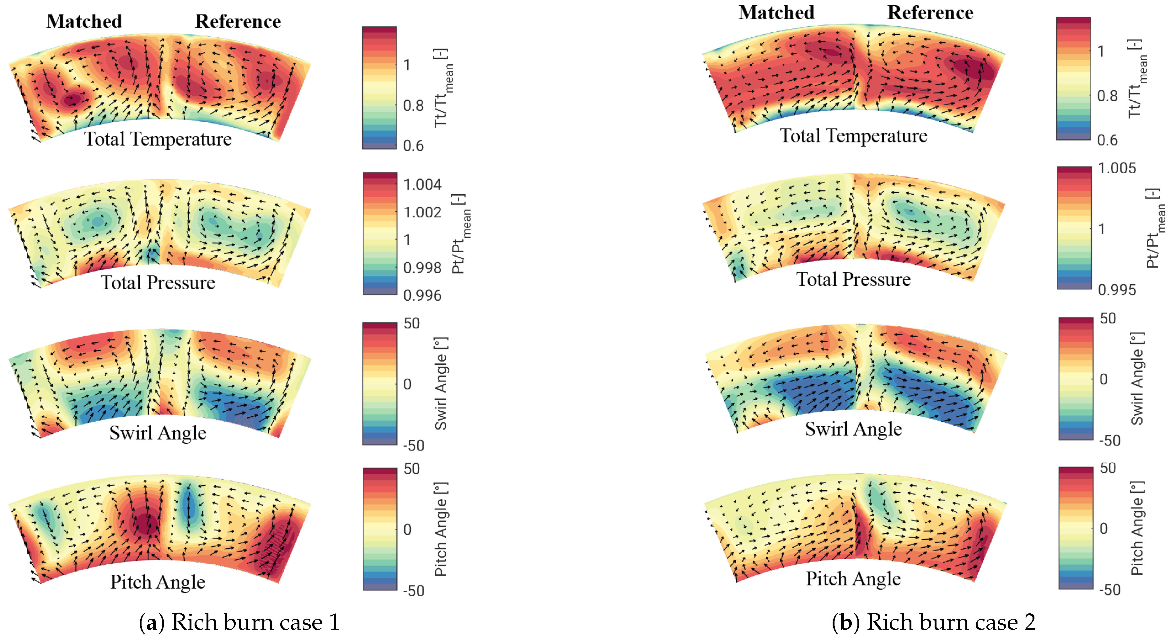
Appendix B.2. Rich Burn Test Cases

The traverses shown in Figure A4 result from the design process of a rich burn combustor. The relatively high swirl angles are caused by a circumferential offset of the quenching ports.
Figure A4. Results of additional rich burn test cases.
Ijtpp 02 00020 g0a4

Appendix C. Influence of Inlet Turbulence Distribution

In order to estimate the effect of an erroneous representation of turbulent quantities on the evaluated results, a simulation using the reference BC for pressure, temperature, and flow angles and the parameterised fields for the turbulent quantities was compared with the reference quantities. Results are shown in Figure A5 as 2D distributions of relative differences and a histogram plot displaying which fractions of the surface show a certain error level. It can be seen that differences in adiabatic wall temperature are below 10% on 98% of the surface, whereas differences in N u can locally reach up to 100% due to an influence on the horseshoe vortex of the left vane. High differences in N u are restricted to the front part due to the acceleration of the flow, whereas the rear part and the vane surfaces, which are more critical with respect to film cooling, show a difference mostly below 20%.
Figure A5. Effect of error in inlet turbulence distribution. Ad.: Adiabatic.
Ijtpp 02 00020 g0a5

References

  1. Klapdor, E.V. Simulation of Combustor-Turbine Interaction in a Jet Engine. Ph.D. Thesis, TU Darmstadt, Darmstadt, Germany, 2011. [Google Scholar]
  2. Chana, K.; Cardwell, D.; Jones, T. A Review of the Oxford Turbine Research Facility. In Proceedings of the ASME Turbo Expo 2013: Turbine Technical Conference and Exposition, San Antonio, TX, USA, 3–7 June 2013; p. GT2013-95687. [Google Scholar]
  3. Povey, T.; Qureshi, I. Developments in hot streak simulators for turbine testing. ASME J. Turbomach. 2009, 121, 031009. [Google Scholar] [CrossRef]
  4. Krichbaum, A.; Werschnik, H.; Wilhelm, M.; Schiffer, H.P.; Lehmann, K. A Large Scale Turbine Test Rig for the Investigation of High Pressure Turbine Aerodynamics and Heat Transfer with variable Inflow Conditions. In Proceedings of the ASME Turbo Expo 2015: Turbine Technical Conference and Exposition, Montreal, QC, Canada, 15–19 June 2015; p. GT2015-43261. [Google Scholar]
  5. Cha, C.M.; Hong, S.; Ireland, P.T.; Denman, P.; Savarianandam, V. Experimental and Numerical Investigation of Combustor-Turbine Interaction Using an Isothermal, Nonreacting Tracer. J. Eng. Gas Turb. Power 2016, 134, 081501. [Google Scholar] [CrossRef]
  6. Hall, B.F.; Chana, K.S.; Povey, T. Design of a Nonreacting Combustor Simulator With Swirl and Temperature Distortion With Experimental Validation. J. Eng. Gas Turb. Power 2014, 136, 081501. [Google Scholar] [CrossRef]
  7. Vagnoli, S.; Verstraete, T. Numerical Study of the Combustor-Turbine Interaction Using Coupled Unsteady Solvers. In Proceedings of the 22nd International Association of Air Breathing Engines (ISABE), Phoenix, Az, USA, 25–30 October 2015. [Google Scholar]
  8. Raynaud, F.; Eggels, R.L.G.M.; Staufer, M.; Sadiki, A.; Janicka, J. Towards Unsteady Simulation of Combustor-Turbine Interaction Using an Integrated Approach. In Proceedings of the ASME Turbo Expo 2015: Turbine Technical Conference and Exposition, Montreal, QC, Canada, 15–19 June 2015; p. GT2015-42110. [Google Scholar]
  9. Koupper, C.; Bonneau, G.; Gicquel, L.; Duchaine, F. Large Eddy Simulations of the Combustor Turbine Interface: Study of the Potential and Clocking Effects. In Proceedings of the ASME Turbo Expo 2016: Turbomachinery Technical Conference and Exposition, Seoul, Korea, 13–17 June 2016; p. GT2016-56443. [Google Scholar]
  10. Munk, M.; Prim, R. On the Multiplicity of Steady Gas Flows Having the Same Streamline Pattern. Proc. Natl. Acad. Sci. USA 1947, 33, 1–8. [Google Scholar] [CrossRef]
  11. Kerrebrock, J.L.; Mikolajczak, A.A. Intra-Stator Transport of Rotor Wakes and Its Effects on Compressor Performance. ASME J. Energy Power 1970, 92, 359–368. [Google Scholar] [CrossRef]
  12. Ong, J.; Miller, R.J. Hot Streak and Vane Coolant Migration in a Downstream Rotor. ASME J. Turbomach. 2012, 134, 051002. [Google Scholar] [CrossRef]
  13. Tallman, J.A. Unsteady Half-Annulus Computational Fluid Dynamics Calculations of Thermal Migration Through a Cooled 2.5 Stage High-Pressure Turbine. ASME J. Turbomach. 2014, 136, 081012. [Google Scholar] [CrossRef]
  14. Giller, L.; Schiffer, H.P. Interactions Between the Combustor Swirl and the High Pressure Stator of a Turbine. In Proceedings of the ASME Turbo Expo 2012: Turbine Technical Conference and Exposition, Copenhagen, Denmark, 11–15 June 2012; p. GT2012-69157. [Google Scholar]
  15. Qureshi, I.; Smith, A.D.; Povey, T. HP Vane Aerodynamics and Heat Transfer in the Presence of Aggressive Inlet Swirl. ASME J. Turbomach. 2013, 135, 021040. [Google Scholar] [CrossRef]
  16. Schmid, G. Effects of Combustor Exit Flow an Turbine Performance and Heat Transfer. Ph.D. Thesis, TU Darmstadt, Darmstadt, Germany, 2014. [Google Scholar]
  17. Beard, P.F.; Smith, A.D.; Povey, T. Effect of Combustor Swirl on Transonic High Pressure Turbine Efficiency. ASME J. Turbomach. 2014, 136, 011002. [Google Scholar] [CrossRef]
  18. Insinna, M.; Griffini, D.; Salvadori, S.; Martelli, F. Effect of Realistic Inflow Conditions an the Aero-Thermal Performance of a Film-Cooled Vane. In Proceedings of the 11th European Turbomachinery Conference, Jyvaskyla, Finland, 25–27 May 2015. [Google Scholar]
  19. Jacobi, S.; Mazzoni, C.; Chana, K.; Rosic, B. Investigation of Unsteady Flow Phenomena in First Vane Caused by Combustor Flow with Swirl. In Proceedings of the ASME Turbo Expo 2016: Turbomachinery Technical Conference and Exposition, Seoul, Korea, 13–17 June 2016; p. GT2016-57358. [Google Scholar]
  20. He, L.; Haller, B.R. Influence of Hot Streak Circumferential Length-Scale in Transonic Turbine Stage. In Proceedings of the ASME Turbo Expo 2004: Power for Land, Sea, and Air, Vienna, Austria, 14–17 June 2004; p. GT2004-53370. [Google Scholar]
  21. Basol, A.M.; Jenny, P.; Ibrahim, M.; Kalfas, A.I.; Abhari, R.S. Hot Streak Migration in a Turbine Stage: Integrated Design to Improve Aerothermal Performance. J. Eng. Gas Turb. Power 2011, 133, 061901. [Google Scholar] [CrossRef]
  22. Beard, P.F.; Smith, A.; Povey, T. Impact of Severe Temperature Distortion on Turbine Efficiency. ASME J. Turbomach. 2013, 135, 011018. [Google Scholar] [CrossRef]
  23. Fossen, G.J.V.; Bunker, R.S. Augmentation of Stagnation Region Heat Transfer Due to Turbulence from a DLN Can Combustor. ASME J. Turbomach. 2001, 123, 140–146. [Google Scholar] [CrossRef]
  24. Khanal, B.; He, L.; Northall, J.; Adami, P. Analysis of Radial Migration of Hot-Streak in Swirling Flow Through High-Pressure Turbine Stage. ASME J. Turbomach. 2013, 135, 041005. [Google Scholar] [CrossRef]
  25. CFX5. Solver Theory Guide. Release 17.0; ANSYS: Canonsburg, PA, USA, 2016. [Google Scholar]
  26. Gupta, A.K.; Lilley, D.G. Swirl Flows; Abacus Press: Tunbridge Wells, UK, 1985. [Google Scholar]
  27. MATLAB. Global Optimization Toolbox User’s Guide; The Math Works: Natick, MA, USA, 2016. [Google Scholar]
  28. Menter, F.R. Two-Equation Eddy-Viscosity Turbulence Models for Engineering Applications. AIAA J. 1994, 32, 1598–1605. [Google Scholar] [CrossRef]
  29. Klinger, H.; Lazik, W.; Wunderlich, T. The Engine 3E Core Engine. In Proceedings of the ASME Turbo Expo 2008: Power for Land, Sea, and Air, Berlin, Germany, 9–13 June 2008; p. GT2008-50679. [Google Scholar]
  30. Hilgert, J.; Bruschewski, M.; Werschnik, H.; Schiffer, H.P. Numerical Studies on Combustor-Turbine Interaction at the Large Scale Turbine Rig (LSTR). In Proceedings of the ASME Turbo Expo 2017: Turbomachinery Technical Conference and Exposition, Charlotte, NC, USA, 16–30 June 2017; p. GT2017-64504. [Google Scholar]
Figure 1. Structure of the interface parameterisation algorithm. CFD: computational fluid dynamics.
Ijtpp 02 00020 g001
Figure 2. Generation of the in-plane velocity field.
Ijtpp 02 00020 g002
Figure 3. Swirler vortex modelling: (a) A single Lamb-Oseen vortex with vectors penetrating the end walls and non-periodic sector boundaries and (b) a system of vortices with periodic sector boundaries and no radial velocity component at the end walls. NGV: nozzle guide vane.
Ijtpp 02 00020 g003
Figure 4. Periodicity of boundaries.
Ijtpp 02 00020 g004
Figure 5. Vortex scaling.
Ijtpp 02 00020 g005
Figure 6. Parameterisation of the temperature field. RTDF: radial temperature distortion factor.
Ijtpp 02 00020 g006
Figure 7. Generation of the temperature field.
Ijtpp 02 00020 g007
Figure 8. Comparison of parameterisaton with a benchmark combustor CFD interface.
Ijtpp 02 00020 g008
Figure 9. CFD domain and y + distribution.
Ijtpp 02 00020 g009
Figure 10. Results of the mesh refinement study. Mio: million, BC: boundary condition.
Ijtpp 02 00020 g010
Figure 11. Isentropic stage efficiency and inlet conditions.
Ijtpp 02 00020 g011
Figure 12. Comparison of adiabatic wall temperature.
Ijtpp 02 00020 g012
Figure 13. Inclusion of combustor wall film cooling.
Ijtpp 02 00020 g013
Figure 14. Comparison of the Nusselt number.
Ijtpp 02 00020 g014
Table 1. Topology and mesh information.
Number ofNumber ofy + MinimalMaximal
PassagesElementsMaximumAverageAnglesAspect Ratio
Stator23.757 Mio.53.061.7517.1 ° 384
Rotor12.417 Mio.26.072.2015.0 ° 504

