Effects of the Approximations Embodied in the Momentum Theory as Applied to the NREL PHASE VI Wind Turbine ^†

Abstract

This paper investigates the impact of the standard approximations embodied in the well-known Momentum Theory on its performance prediction capabilities. To this aim, the results of the momentum theory, which is still widely used in all Blade Element/Momentum codes for the analysis and/or design of wind turbines, are compared with those obtained with an actuator disk model based on Computational Fluid Dynamics techniques. In this method, the axisymmetric and steady Euler equations are solved with a classical finite volume approach, while the turbine effects are modelled through a set of axial and tangential body forces distributed over a disk shaped region representing the rotor swept surface. Since this method does not rely on the momentum theory simplifying assumptions, it can be suitably employed to verify the momentum theory validity. The analysis is carried out using the well documented experimental data of the National Renewable Energy Laboratory Phase VI wind turbine.

1. Introduction

Nowadays, the performance analysis and design of wind turbines are frequently carried out by coupling a through-flow with a blade-to-blade method. Since wind turbines are characterised by a very low solidity, especially due to the low value of the blade number and to the high rotor radius, a typical blade-to-blade approach is the so-called Blade Element Theory (BET). In the latter, the blade is discretised into several elements in the spanwise direction. Then, the forces exercised by each blade element on the fluid are evaluated with a 2D approach, that is on the basis of the 2D wing section characteristics corrected for dynamic stall effects.

Coming now to the through-flow, it is often simulated with the help of the inviscid actuator disk (AD) concept, i.e., an infinitesimal-width disk which models the turbine presence by introducing a jump in the static pressure and in the tangential velocity across it. There are several approaches to solve the flow equations around an AD. One of these approaches is based on the use of classical Computational Fluid Dynamics (CFD) techniques [1,2,3,4] and for this reason it will be named CFD-AD [5,6,7,8,9,10,11]. In this method, the Euler (or Navier–Stokes) equations are solved by finite volume or difference schemes, while the presence of the turbine is modelled by activating the momentum source terms in a disk-shaped region. These source terms are often evaluated by coupling the CFD code with a BET module. Note that the CFD-AD method relies on the exact flow equations and it introduces only the discretisation errors which, however, can be easily controlled through a grid refinement study.

The second AD approach, which originates from the work of Wu [12], is the so-called nonlinear and semi-analytical actuator disk (SA-AD). This method has been mainly developed by Conway [13] and extended to rotors with a finite hub or a duct in [14,15,16,17,18,19]. The SA-AD is also based on the exact flow equations and it only introduces a few numerical errors embodied in the semi-analytical solution procedure. An analysis of these errors is reported in [20,21,22].

Finally, the most known and simple AD method is that based on the Momentum Theory (MT) which, coupled with the BET, gives rise to the well-known Blade Element/Momentum theory (BEM) constituting the most important and employed tool for the analysis and design of wind turbines (see for example [23,24,25,26,27,28,29,30,31,32]). Based on a very simplified version of the inviscid, incompressible, steady and axysimmetric flow equations, the MT returns two algebraic equations which express the axial and tangential body forces as a function of the flow field at the disk. However, these equations are obtained by means of two simplifying assumptions. The first one is the linearisation of the swirl terms [33] and the second one is the use of the axial momentum equation in a wrong differential form [23,34]. In particular, Goorjian [35] proved that this differential form is wrong because it leads to a contradiction when combined with the other equations of the MT.

Due to the large diffusion of the BEM methods, the evaluation of the MT errors is of the utmost importance; consequently, a few works dealing with this issue have recently appeared [36,37,38,39,24,40,41]. These studies present the comparison between the MT and AD methods based on flow equations not polluted by the typical MT approximations, e.g., CFD-AD and SA-AD. Moreover, these works mainly evaluate the MT errors for the unphysical radially uniform load distribution. Contrariwise, in the present paper, the errors embodied in the MT are evaluated for a load distribution of a real wind turbine. To this aim, a CFD-AD method is employed to evaluate the axial and tangential body forces of the well-documented NREL Phase VI wind turbine [42]. The aerodynamic performance of this 10 m-diameter turbine was extensively and experimentally investigated by the National Renewable Energy Laboratory (NREL) at the 24.4 m × 36.6 m wind tunnel of the National Aeronautics and Space Administration (NASA) Ames Research Center. The main objective of this experimental campaign was to provide useful information on the three-dimensional and full-scale aerodynamic behaviour of a wind turbine. Contrary to a full-scale field test, the wind tunnel testing provided the unique opportunity to remove the inflow turbulence and shear flow effects. Consequently, the NREL Phase VI data have been successfully exploited to validate and develop the analysis of several wind turbines and design approaches which often rely on simplified inflow characteristics. These data have also been employed to validate BEM tools (see for instance [43,44,45,46]) with particular attention to the tip loss modelling and to the stall delay effects. However, the errors due to the swirl terms linearisation and to the wrong differential form of the axial momentum equation have never been quantified for a well-documented test case such as the NREL Phase VI turbine. Additionally, the impact of those errors has always been disregarded when analysing the outcome of these validation procedures. For this reason, the evaluation of the MT errors, discussed in this paper, is also aimed at providing a more meaningful interpretation of the BEM validation procedure results.

The paper outline is as follows. The next section briefly introduces the MT equations and their approximations. Then, a CFD-AD approach is developed and validated against experimental data. Finally, the results of the MT and of the CFD-AD method are compared with each other to quantify the errors embodied in the MT for different values of the tip speed ratio.

2. The Momentum Theory

In the MT, the flow is supposed to be stationary, incompressible and inviscid. Moreover, it is also considered axisymmetric; therefore, it is convenient to introduce a cylindrical coordinate system $(z,r,\theta )$. Consequently, the axial, radial and tangential velocities are named $v_z$, $v_r$ and $v_{\theta }$, respectively. The velocity field at upstream infinity is $(v_{z,\infty },0,0)$, where $v_{z,\infty }$ is uniform; therefore, the static pressure $p_{\infty }$ is also uniform there. The subscripts 1 and 2 are used for quantities just ahead and behind the disk, respectively. In particular, the axial and radial velocities at the disk are considered to be uniform across the disk, i.e., $v_{z,1}=v_{z,2}=v_{z,d}$ and $v_{r,1}=v_{r,2}=v_{r,d}$, where the subscript d stands for disk. To simulate the presence of the turbine, a jump in the static pressure and in the tangential velocity is introduced across the disk, i.e., $\Delta p=p_1-p_2>0$ and $\Delta v_{\theta }=v_{\theta ,1}-v_{\theta ,2}>0$. Furthermore, as customary in the wind turbine field, it is also convenient to introduce the axial and tangential induction factors defined as $a=1-v_{z,d}/v_{z,\infty }$ and $a^{\prime }=-v_{\theta ,2}/(2\mathsf{\Omega }r)$, where $\mathsf{\Omega }$ is the rotor angular velocity. At downstream infinity, it can be easily proven that, outside the wake, the velocity field is $(v_{z,\infty },0,0)$ and the static pressure is $p_{\infty }$ [23], whereas, inside the wake, the static pressure, and the axial and tangential velocities vary in the spanwise direction. A subscript w is used for these latter quantities. Moreover, far behind the disk, the radial component of the velocity $v_{r,w}$ and its derivative $\partial v_{r,w}/\partial r$ are assumed to be zero everywhere. Thanks to these last assumptions, it can be proven that, at downstream infinity, the radial momentum equation for a steady, inviscid and axisymmetric flow reduces to

$$\frac{\mathrm{d}{p}_w}{\mathrm{d}r}=\rho \frac{v_{\theta ,w}^2}{r}.$$

(1)

In Equation (1), $\rho$ is the fluid density.

The rotor thrust T can be cast in the following form:

$$T={\int }_{S_d}\Delta p\mathrm{d}S={\int }_{S_d}\rho v_{z,d}(v_{z,\infty }-v_{z,w})\mathrm{d}S+{\int }_{S_w}(p_{\infty }-p_w)\mathrm{d}S,$$

(2)

as it can be easily proven by applying the axial momentum equation (see [23] for details). In the above Equation, $S_d$ and $S_w$ are the cross sections of the streamtube swallowed by the turbine at the disk and at downstream infinity, respectively. Moreover, the pressure jump across the disk can also be evaluated through the Bernoulli principle as applied to the streamtubes ahead of and behind the disk

$$\mathrm{d}T=\Delta p\mathrm{d}{S}_d=\left[\frac{1}{2}\rho \left(v_{z,\infty }^2-v_{z,w}^2\right)+\frac{1}{2}\rho \left(v_{\theta ,2}^2-v_{\theta ,w}^2\right)+p_{\infty }-p_w\right]\mathrm{d}{S}_d.$$

(3)

Equations (1)–(3) are exact, but they do not allow a simple relation to be found between the rotor loads and the velocity field at the disk. For this reason, they are customarily simplified. First of all, Equation (2) is usually employed in the differential form

$$\mathrm{d}T=\rho v_{z,d}(v_{z,\infty }-v_{z,w})\mathrm{d}{S}_d+(p_{\infty }-p_w)\mathrm{d}{S}_w$$

(4)

which, as proven by Goorjian [35], is wrong. Furthermore, the equations are simplified by neglecting all nonlinear tangential velocity terms. By so doing, Equation (1) returns

$$p_w=p_{\infty },$$

(5)

so that Equations (3) and (4) become

$$\begin{array}{cc}\hfill \frac{\mathrm{d}T}{\mathrm{d}r}& =\frac{1}{2}\rho \left(v_{z,\infty }^2-v_{z,w}^2\right)2\pi r\hfill \end{array}$$

(6)

$$\begin{array}{cc}\hfill \frac{\mathrm{d}T}{\mathrm{d}r}& =\rho v_{z,d}(v_{z,\infty }-v_{z,w})2\pi r.\hfill \end{array}$$

(7)

Equating the above two equations, the famous Froude law can be obtained

$$v_{z,d}=\frac{v_{z,\infty }+v_{z,w}}{2}.$$

(8)

With the help of Equation (8), Equation (7) can be expressed as a function of the axial induction factor a through the following well-known relation:

$$\frac{\mathrm{d}T}{\mathrm{d}r}=B{F}_n=\frac{1}{2}\rho v_{z,\infty }^{2}2\pi r4a(1-a).$$

(9)

In the above equation, B is the blade number and $F_n[N/m]$ is the load normal to the disk surface, i.e., the load in the axial direction. Equation (9) can be used to obtain the axial induction factor for a prescribed rotor load. However, due to the two aforementioned simplifying assumptions, only an approximate value of a can be obtained from Equation (9). The latter is one of the two classical MT equations. The second one is obtained by applying the angular momentum equation to the turbine rotor. By doing so, the torque $\mathrm{d}Q$ per unit length reads [23]

$$\frac{\mathrm{d}Q}{\mathrm{d}r}=Br{F}_t=\rho \pi r^3\mathsf{\Omega }{v}_{z,\infty }4a^{\prime }(1-a),$$

(10)

where $F_t[N/m]$ is the tangential load on each blade. The well-known Equation (10) is exact and it can be used to evaluate $a^{\prime }$ once the torque and the axial induction are known. However, if the approximate a value is used, i.e., the a value retrieved from Equation (9), an error is also introduced in $a^{\prime }$.

3. The CFD Actuator Disk Method

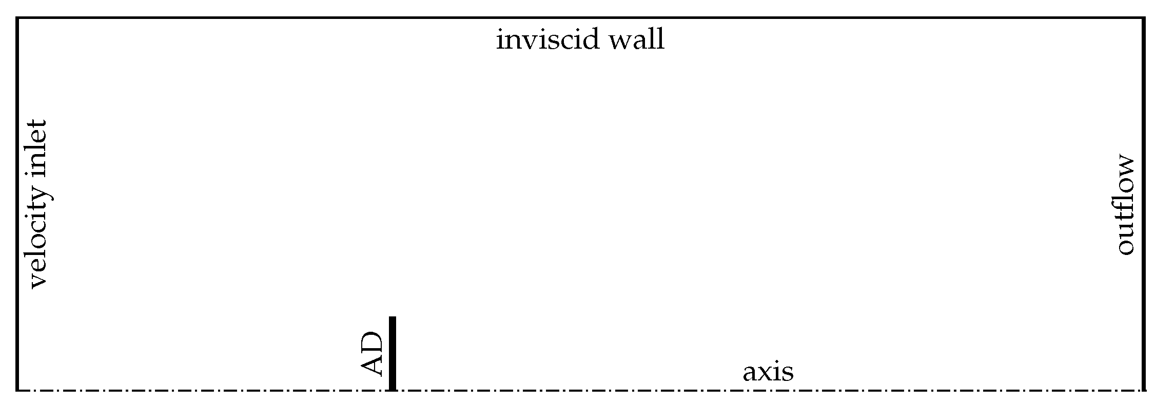
As stressed in the introduction, the CFD-AD is an analysis method aimed at describing the turbine through-flow in a synthetic manner, i.e., by replacing the turbine with an actuator disk. This disk can be regarded as a rotor with infinite blades across which a jump in the static pressure and in the tangential velocity occurs. In particular, the CFD-AD solves the steady, axisymmetric and incompressible Euler equations by finite volume or difference schemes, whereas it models the turbine effects by a set of body forces distributed over the disk. To this aim, the axial and tangential source terms are activated only in the disk region. The 2D-axisymmetric computational domain is shown in Figure 1. The disk is set normal to the free-stream which is modelled by a uniform velocity-inlet boundary condition. The remaining boundary conditions are described in Figure 1. The domain is divided into two regions. The first one, named inner domain, is characterised by a uniformly spaced and highly dense grid, whereas in the second one (the outer domain) this density decreases moving towards the outer boundaries of the overall domain. Both sub-domains are discretised through a structured mesh and a grid dependence analysis is carried out doubling twice the spacing of the inner domain mesh (more details on this issue can be found in [22], where a similar and thorough grid convergence analysis has been presented for the CFD actuator disk method). A pressure-based solver [47] is used to obtain the numerical solution of the axisymmetric Euler equations. In particular, the pressure–velocity coupling is performed through the well-known SIMPLE segregated algorithm [1], while the QUICK [48] scheme is employed for spatial discretisations of the momentum equation.

Note that the CFD-AD is an axisymmetric approach; therefore, once the body forces distribution has been prescribed at the disk, the CFD code returns the azimuthally averaged flow field, i.e., the a and $a^{\prime }$ distributions have to be considered as azimuthally averaged. As customary, the axial and tangential induction factors are corrected through the well-known Prandtl F factor to give [23]

$$a_B=a/F\mathrm{and}{a}_B^{\prime }=a^{\prime }/F,$$

(11)

where $a_B$ and $a_B^{\prime }$ are the local induction factors at the blade position and

$$F=\frac{2}{\pi }arccos\left[e^{-\frac{B(R-r)}{2rsin\varphi }}\right].$$

(12)

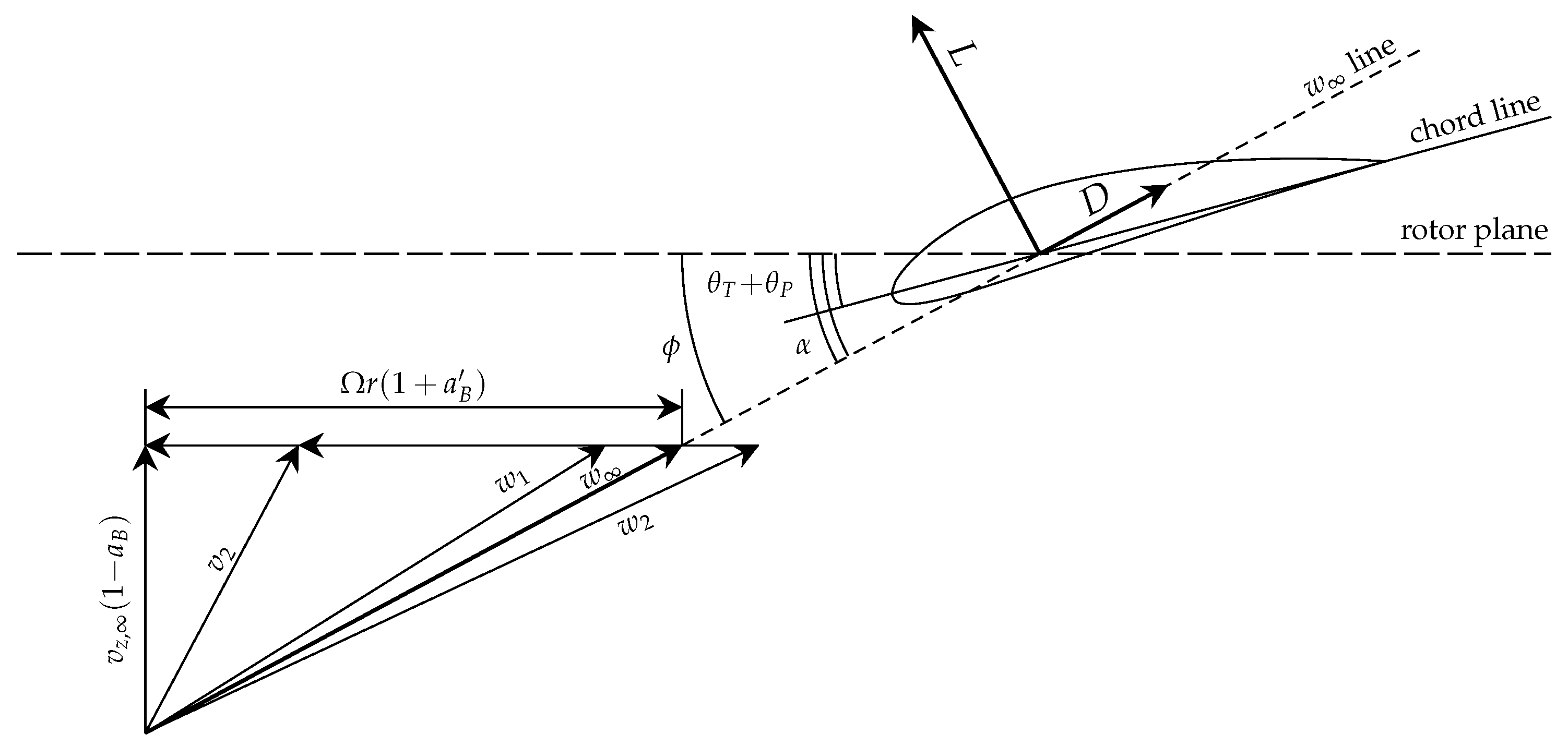
In the above equation, $\varphi$ is the angle between the relative velocity $w_{\infty }$ and the rotor plane (see Figure 2). In particular, $w_{\infty }$ is defined as the vectorial mean between the relative velocities at the inlet and at the outlet of the rotor, i.e., $w_{\infty }=\frac{1}{2}(w_1+w_2$). Moreover, the flow angle $\varphi$ can also be related to the blade induction factors through the following simple geometrical relation (see Figure 2):

$$\varphi =arctan\left(\frac{1}{{\lambda }_r}\frac{1-a_B}{1+a_B^{\prime }}\right),$$

(13)

where ${\lambda }_r=\mathsf{\Omega }r/v_{z,\infty }$ is the local speed ratio. Obviously, the $w_{\infty }$ magnitude is

$$w_{\infty }^2={\left[v_{z,\infty }(1-a_B)\right]}^2+{\left[\mathsf{\Omega }r(1+a_B^{\prime })\right]}^2.$$

(14)

As customary, the body forces are evaluated through a blade-element approach, namely the blade is divided into N elements in the spanwise direction and the forces on each element are evaluated on the basis of the 2D wing section characteristics corrected for dynamic stall effects. Referring to Figure 2, it is easy to prove that the normal and tangential loads read

$$\begin{array}{cc}\hfill F_n& =\frac{1}{2}\rho c{w}_{\infty }^2{F}_1(C_{L}cos\varphi +C_{D}sin\varphi ),\hfill \end{array}$$

(15)

$$\begin{array}{cc}\hfill F_t& =\frac{1}{2}\rho c{w}_{\infty }^2{F}_1(C_{L}sin\varphi -C_{D}cos\varphi ),\hfill \end{array}$$

(16)

where c is the local chord, $C_L$ (resp. $C_D$) is the section lift (resp. drag) coefficient defined as $C_L=L/(\frac{1}{2}\rho w_{\infty }^{2}c)$ (resp. $C_D=D/(\frac{1}{2}\rho w_{\infty }^{2}c)$) and L (resp. D) is the 2D wing section lift (resp. drag).

Moreover, the loads are further corrected to take into account the pressure equalisation occurring at the blade tip. To this aim, the correction factor $F_1$ [49] has also been introduced in Equations (15) and (16). The $F_1$ factor is defined as

$$F_1=\frac{2}{\pi }arccos\left[e^{-g\frac{B(R-r)}{2rsin\varphi }}\right],$$

(17)

where $g=exp[-c_1(B\lambda -c_2)]+0.1$ and $\lambda$ is the tip speed ratio $\lambda =\mathsf{\Omega }R/v_{z,\infty }$. The empirical coefficients $c_1$ and $c_2$ are set equal to 0.125 and 21, respectively.

The solution procedure can be summarised as follows. A starting distribution of loads is guessed or obtained from previous computations. Then, the body forces acting on the elementary volume $\mathrm{d}V=2\pi r\mathrm{d}r\mathrm{d}z$ are evaluated as

$$f_n=\frac{F_n}{2\pi r\mathrm{d}z}\mathrm{and}{f}_t=\frac{F_t}{2\pi r\mathrm{d}z}.$$

(18)

These body forces are prescribed at the disk region and the CFD simulation is run updating the body forces at each iteration. More in detail, the a and $a^{\prime }$ distribution is obtained from the CFD code. Then, Equations (11) and (13) are substituted in (12) to give

$$F-\frac{2}{\pi }arccos\left\{exp\left[-\frac{B(R-r)}{2rsin\left(arctan\left(\frac{1}{{\lambda }_r}\frac{1-a/F}{1+a^{\prime }/F}\right)\right)}\right]\right\}=0$$

(19)

which is a nonlinear equation to be numerically solved for F. Once F has been computed, $a_B$, $a_B^{\prime }$ and $w_{\infty }$ can be easily evaluated through Equations (11) and (14). Consequently, $\varphi$ and $F_1$ are obtained from Equations (13) and (17). Then, the angle of attack $\alpha$ is given by $\alpha =\varphi -{\theta }_T-{\theta }_P$, where ${\theta }_T$ and ${\theta }_P$ are the twist and pitch angle, respectively. Once $\alpha$ is known, $C_L$ and $C_D$ can be evaluated from the tabulated 2D airfoil data and the loads are updated through Equations (15) and (16). The procedure is repeated at each iteration of the CFD code until convergence.

4. Validation of the CFD-AD Method

In this section, the performance of the stall regulated NREL Phase VI wind turbine [42] will be investigated through the CFD-AD and the MT. This two-bladed, 10 m-diameter turbine has a rated power of 20 kW and it is characterised by a linear taper and a nonlinear twist distribution. The turbine is equipped with a full-span pitch control and the S809 airfoil has been exclusively employed from hub to tip. The experimental campaign was conducted in the 24.4 m × 36.6 m wind tunnel of the NASA Ames Research Center for a free stream velocity in the range [5, 25] m/s and for a rotational speed equal to 71.93 rpm. In addition to the rotor power, other very important quantities were acquired during the tests, such as the blade surface pressure distributions and the inflow dynamic pressure at five span locations, i.e., at 30%, 46.6%, 63.3%, 80% and 95% of the rotor span.

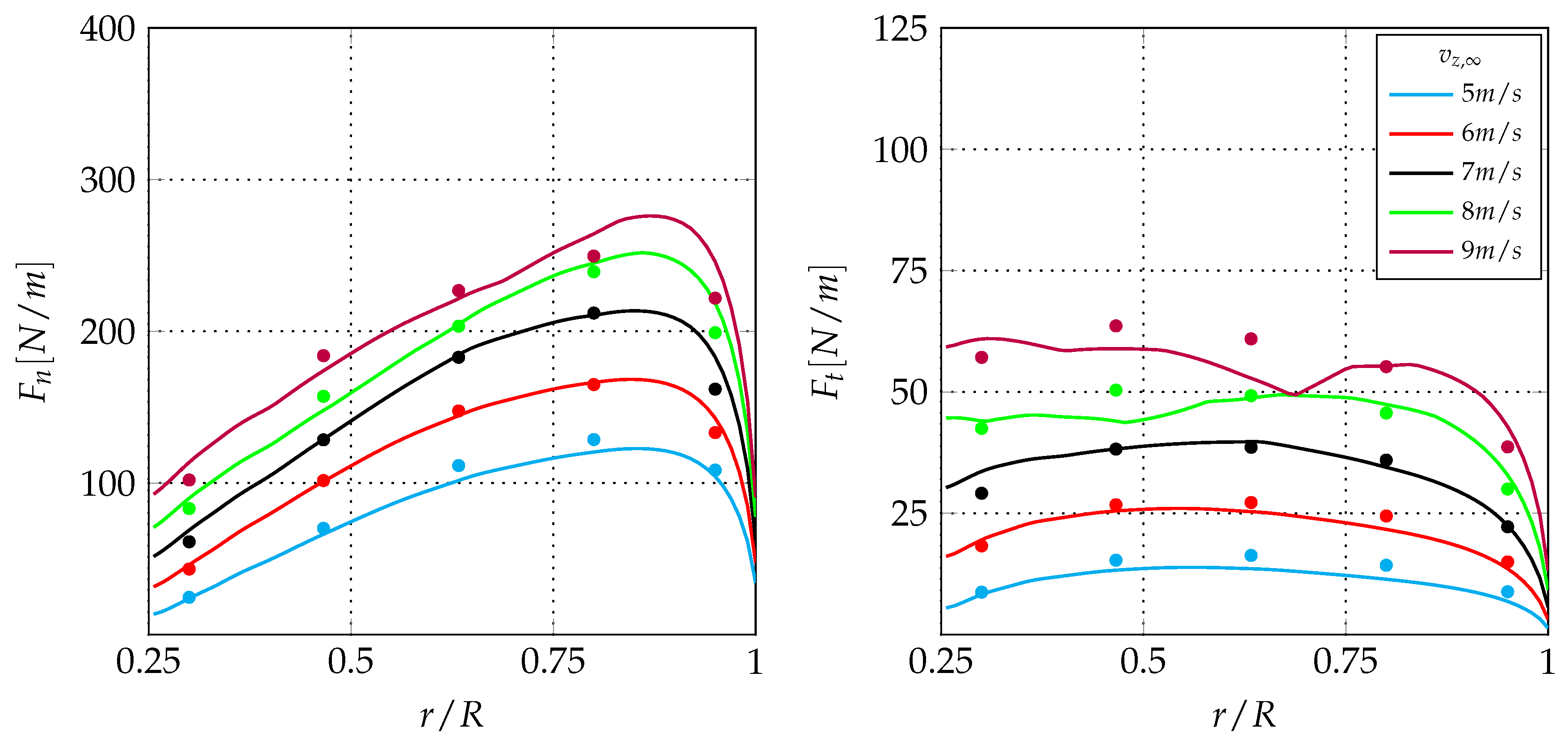
Figure 3 reports the radial distribution of the axial $F_n$ and tangential $F_t$ loads for $v_{z,\infty }=$ 5, 6, 7, 8 and 9 m/s as predicted by the CFD-AD method. The results are compared with the experimental data showing a very good agreement for $v_{z,\infty }=$ 5, 6, 7, and 8 m/s. When the wind speed is increased, the angle of attack also increases along the blade and a stall phenomenon could take place. For stalled blades, all methods based on the actuator disk concept fail to properly model the flow physics unless a tuning procedure is carried out for the airfoils data [43]. In fact, the flow becomes three-dimensional in the presence of the stall, thus violating the main assumptions of the actuator disk approach. Hence, it is not surprising that the results of the CFD-AD differ to some extent from the experimental data for high values of the wind speed. However, this part of the operating envelop is not of interest for the purposes of the present paper, i.e., the evaluation of the MT errors. In fact, as shown in the forthcoming and in Sørensen [24], Madsen et al. 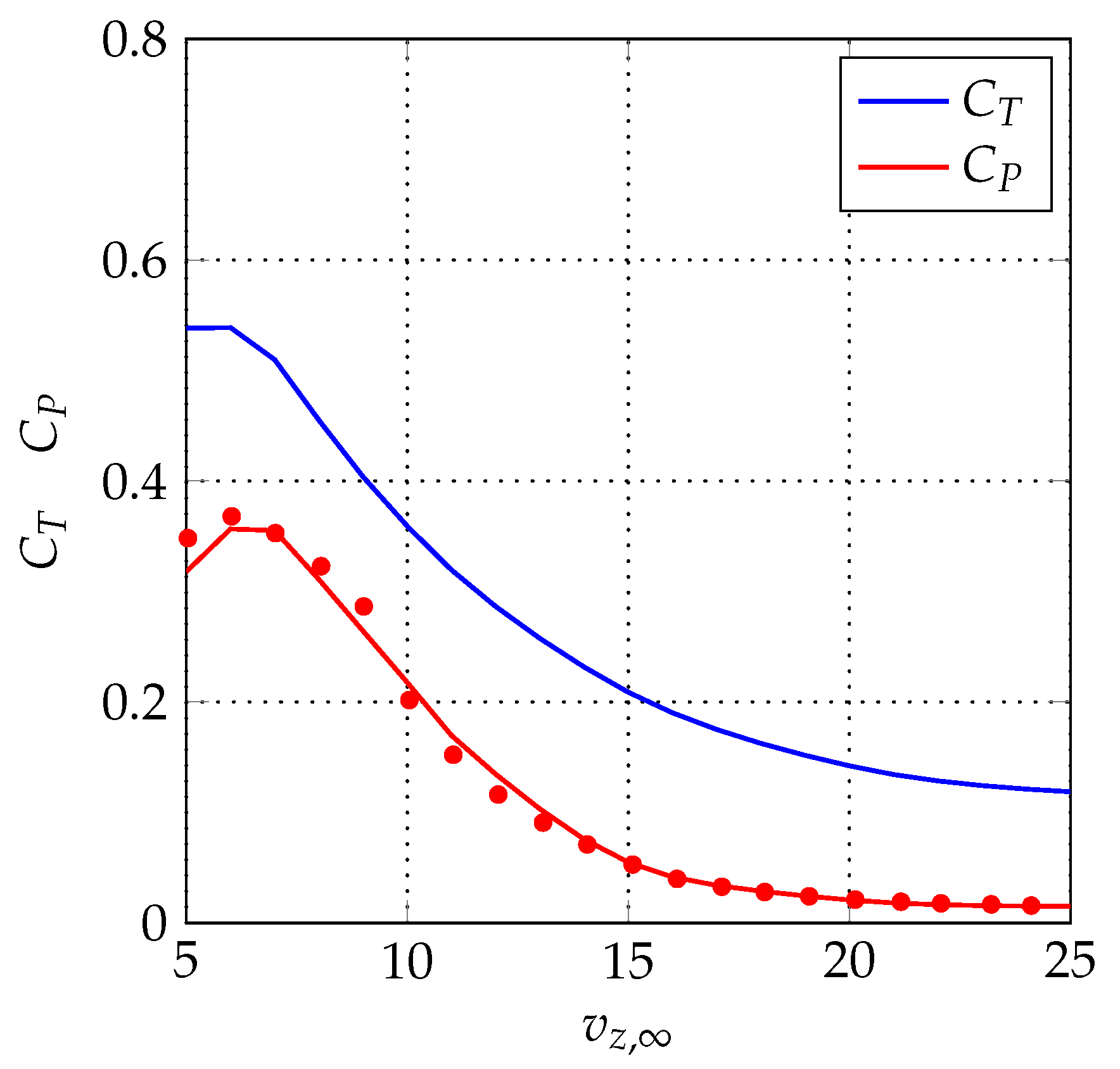[38], Bontempo and Manna [41], the higher values of these errors are related to high values of the thrust coefficient $C_T=T/(\frac{1}{2}\rho v_{z,\infty }^2\pi R^2)$ which are attained for low wind speeds. This can also be seen in Figure 4 which shows the thrust $C_T$ and the power $C_P=P/(\frac{1}{2}\rho v_{z,\infty }^3\pi R^2)$ coefficients as a function of the wind speed. The figure clearly shows that $C_T$ increases by decreasing the wind speed. In the same figure, the experimental values of the power coefficient are also reported for validation purposes.

5. Evaluation of the Momentum Theory Errors

In the previous section, it has been shown that, for stall-free conditions, the CFD-AD method reproduces well the axial and tangential loads of the NREL Phase VI wind turbine. Moreover, since this method is not affected by the typical errors of the MT, its results can be confidently assumed as a reference to quantify these errors. To this aim, for a prescribed value of the wind speed $v_{z,\infty }$ and of the angular velocity $\mathsf{\Omega }$, the axial and tangential induction factors are computed both with the CFD-AD and the MT, and then compared with each other. 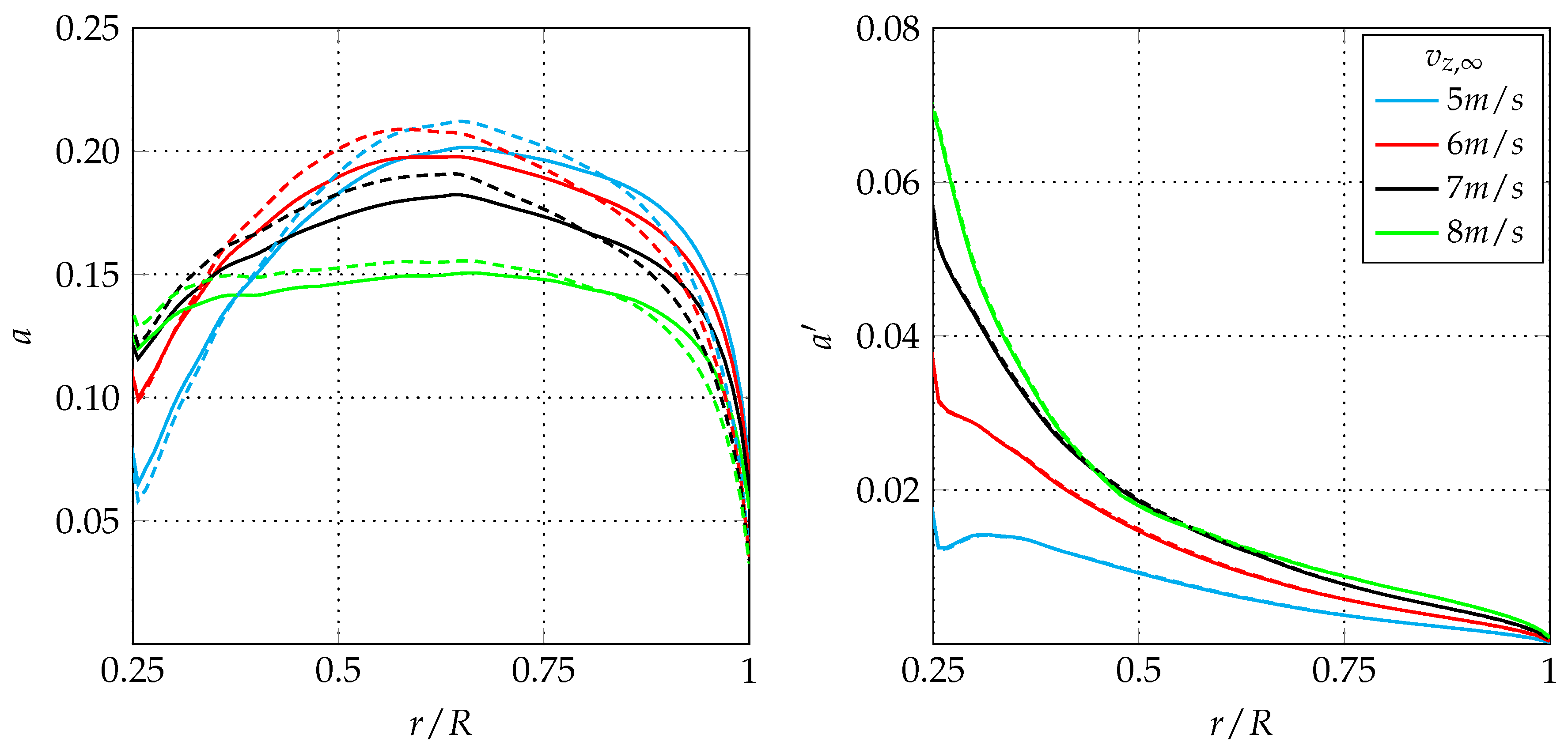More in detail, for the load distributions reported in Figure 3, the a and $a^{\prime }$ distributions as predicted by the MT are evaluated through Equations (9) and (10), respectively. These distributions are reported in Figure 5 and compared with those obtained with the CFD-AD method.

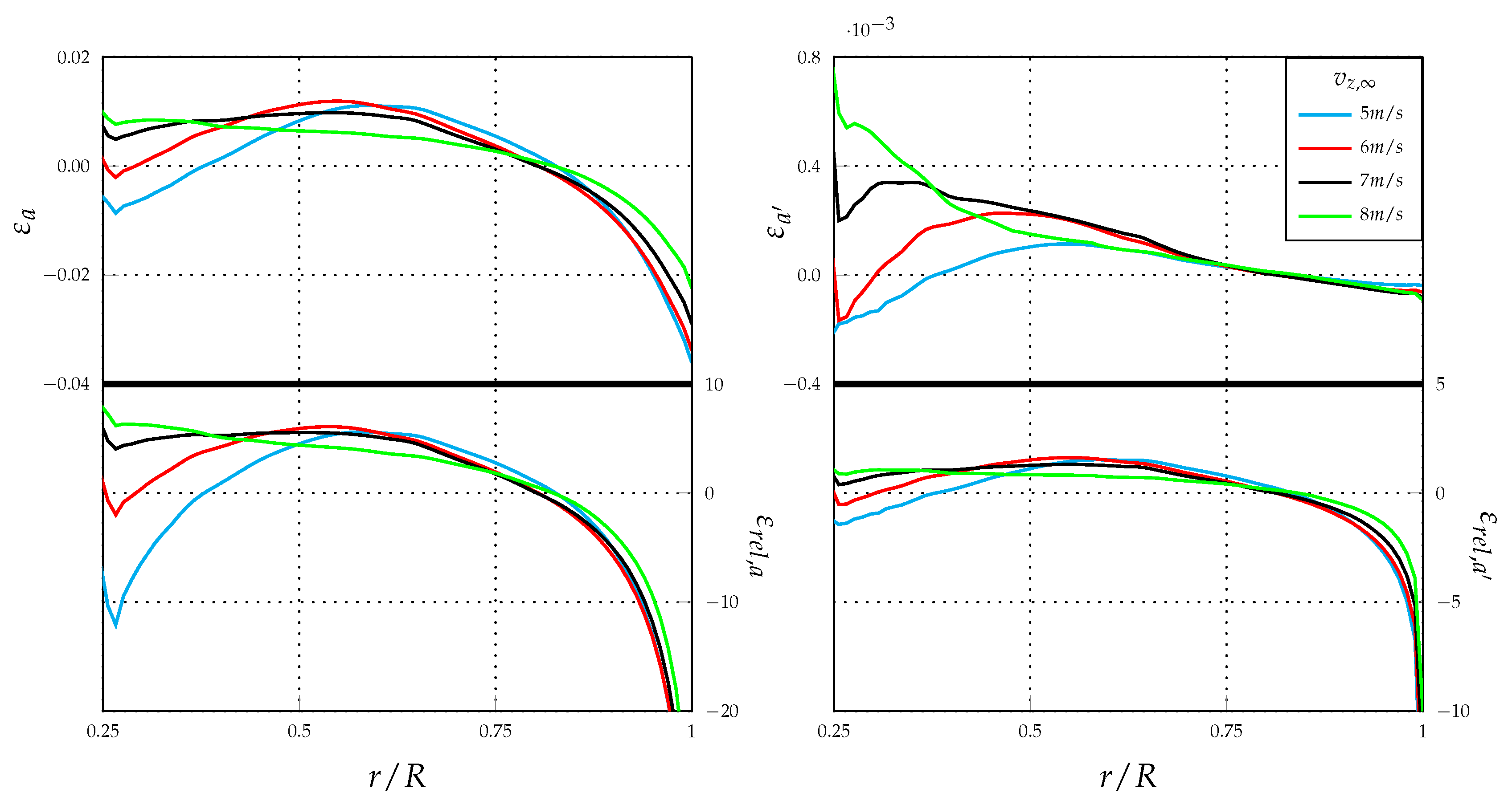
Moreover, Figure 6-left (resp. right) represents the absolute ${\epsilon }_a$ (resp. ${\epsilon }_{a^{\prime }}$) and relative ${\epsilon }_{rel,a}=100\times {\epsilon }_a/a$ (resp. ${\epsilon }_{rel,a^{\prime }}=100\times {\epsilon }_a^{\prime }/a^{\prime }$) errors associated to the axial (resp. tangential) induction factor. As clearly shown, contrary to the common belief, the errors in a are considerable and, in agreement with [24,38,40], they generally increase with the thrust coefficient, i.e., decreasing the wind speed. Furthermore, it can also be observed that the high errors in a do not significantly affect the $a^{\prime }$ evaluation. In fact, as shown in Figure 5, the MT and CFD-AD distributions of the tangential induction factor are very close to each other all along the blade and independently of the thrust coefficient value. More in detail, for all analysed cases, the absolute error in a (see Figure 6-left) reaches its maximum value at the tip. This maximum value is generally in the range [−0.04, −0.02]. The absolute errors in ${\epsilon }_{a^{\prime }}$ are very small and, as quantified in Figure 6-right, they are of the order ${10}^{-3}$. Coming now to the relative errors reported in the bottom panels of Figure 6, it can be appreciated that ${\epsilon }_{rel,a}$ and ${\epsilon }_{rel,a^{\prime }}$ are about 10% and a few percent, respectively. Moreover, both of them exhibit a singular behaviour at the tip. In fact, a vertical asymptote exists for $r/R\to 1$ because either the axial or tangential induction factors go to zero at the tip, while the absolute errors ${\epsilon }_{rel,a}$ and ${\epsilon }_{rel,a^{\prime }}$ have a finite value there.

Finally, it should be noted that the momentum theory is generally employed only at those radial stations where a is lower than a critical value $a_c$, whereas an empirical correction is adopted elsewhere. A classical value for $a_c$ is 1/3, which is used in the very popular Glauert [23] empirical relation. Looking at Figure 5, it can be easily understood that the highlighted momentum theory errors cannot be avoided using an empirical correction, since, for all analysed cases, the axial induction factor is always lower than $a_c=1/3$ all along the rotor span.

Up to now, only the local errors of the momentum theory have been analysed. However, it is also useful to study the effect of these errors on the accuracy of global quantities (such as the mass flow rate $\dot{m}$ swallowed by the rotor), as predicted by the momentum theory. First of all, note that, although differences in the a and $a^{\prime }$ distribution exist, the CFD-AD method and the MT must return the same values for the power and the thrust coefficient. This is because the same $F_n$ and $F_t$ (see Figure 3) have been employed in the two methods. The $a^{\prime }$ error is proportional to the error in the specific work W since, as it can be readily obtained by the angular momentum equation, $W=2{\mathsf{\Omega }}^2{r}^2{a}^{\prime }$. The error in a is related to the error in the overall mass flow rate through the rotor. In fact, elaborating the $\dot{m}$ definition

$$\dot{m}={\int }_0^R\rho v_{z,\infty }(1-a)2\pi r\mathrm{d}r,$$

the difference between the mass flow rate evaluated by the MT (${\dot{m}}_{\mathrm{MT}}$) and the CFD-AD method (${\dot{m}}_{\mathrm{CFD}}$) can be expressed as

$$\frac{{\dot{m}}_{\mathrm{MT}}-{\dot{m}}_{\mathrm{CFD}}}{\rho v_{z,\infty }\pi R^2}=-({\overline{a}}_{\mathrm{MT}}-{\overline{a}}_{\mathrm{CFD}}).$$

In the above equation, ${\overline{a}}_{\mathrm{MT}}$ and ${\overline{a}}_{\mathrm{CFD}}$ are the area-averaged value of the a distribution as predicted by the MT and the CFD-AD, respectively. Before starting the discussion on the mass flow rate error, note that, as shown in Figure 5 and Figure 6, the MT always underestimates the axial induction in the tip region, while it overestimates a in the midspan region. When integrated over the whole span, the underestimated and overestimated contributions to the overall mass flow rate compensate each other; therefore, the difference between ${\dot{m}}_{MT}$ and ${\dot{m}}_{CFD}$ becomes small (see

Table 1. Error analysis on the mass flow swallowed by the turbine.

	${\mathit{v}}_{\mathit{z},\infty }$ = 5 m/s	${\mathit{v}}_{\mathit{z},\infty }$ = 6 m/s	${\mathit{v}}_{\mathit{z},\infty }$ = 7 m/s	${\mathit{v}}_{\mathit{z},\infty }$ = 8 m/s
${\overline{a}}_{MT}$	0.16972	0.16947	0.15758	0.13658
${\overline{a}}_{CFD}$	0.17125	0.17023	0.15759	0.13622
$100\times \frac{{\overline{a}}_{MT}-{\overline{a}}_{CFD}}{{\overline{a}}_{CFD}}$	−0.89535	−0.44954	0.01004	0.26738

), i.e., the global performance prediction is loosely influenced by the significant local errors in the axial induction factor.

6. Conclusions

The impact of the errors embodied in the momentum theory has been evaluated for the well-documented NREL Phase VI wind turbine for which a large highly accurate experimental database is available. These errors are due to the linearisation of the swirl terms and to the use of the axial momentum equation in an approximate form. Their quantification has been carried out by comparing the MT results with those of a validated CFD-AD approach which does not rely on the same simplifying assumptions of the MT. Contrary to the common belief, these errors are not negligible at all in terms of the axial induction factor. In particular, in the analysed case, it has been shown that the MT underestimates the axial induction factor a near the tip region and overestimates it in the middle span region. Contrariwise, no significant errors arise in the tangential induction factor. Finally, the findings reported in this paper provide a more meaningful interpretation of the BEM validation procedures which always disregard the impact of the aforementioned errors on the results.