Semi-Supervised Deep Learning Framework for Predictive Maintenance in Offshore Wind Turbines ^†

Abstract

The increasing deployment of wind energy systems, particularly offshore wind farms, necessitates advanced monitoring and maintenance strategies to ensure optimal performance and minimize downtime. Supervisory Control And Data Acquisition (SCADA) systems have become indispensable tools for monitoring the operational health of wind turbines, generating vast quantities of time series data from various sensors. Anomaly detection techniques applied to this data offer the potential to proactively identify deviations from normal behavior, providing early warning signals of potential component failures. Traditional model-based approaches for fault detection often struggle to capture the complexity and non-linear dynamics of wind turbine systems. This has led to a growing interest in data-driven methods, particularly those leveraging machine learning and deep learning, to address anomaly detection in wind energy applications. This study focuses on the development and application of a semi-supervised, multivariate anomaly detection model for horizontal axis wind turbines. The core of this study lies in Bidirectional Long Short-Term Memory (BI-LSTM) networks, specifically a BI-LSTM autoencoder architecture, to analyze time series data from a SCADA system and automatically detect anomalous behavior that could indicate potential component failures. Moreover, the approach is reinforced by the integration of the Isolation Forest algorithm, which operates in an unsupervised manner to further refine normal behavior by identifying and excluding additional anomalous points in the training set, beyond those already labeled by the data provider. The research utilizes a real-world dataset provided by EDP Renewables, encompassing two years of comprehensive SCADA records collected from a single offshore wind turbine operating in the Gulf of Guinea. Furthermore, the dataset contains the logs of failure events and recorded alarms triggered by the SCADA system across a wide range of subsystems. The paper proposes a multi-modal anomaly detection framework orchestrating an unsupervised module (i.e., decision tree method) with a supervised one (i.e., BI-LSTM AE). The results highlight the efficacy of the BI-LSTM autoencoder in accurately identifying anomalies within the SCADA data that exhibit strong temporal correlation with logged warnings and the actual failure events. The model’s performance is rigorously evaluated using standard machine learning metrics, including precision, recall, F1 Score, and accuracy, all of which demonstrate favorable results. Further analysis is conducted using Cumulative Sum (CUSUM) control charts to gain a deeper understanding of the identified anomalies’ behavior, particularly their persistence and timing leading up to the failures.

1. Introduction

The penetration of wind power in energy networks is gaining momentum in view of the trend in installed capacity, the achievement of sustainability and security of supply being crucial in green energy transitioning roadmaps. Consequently, future decarbonization scenario depends on wind energy exploitation due to a plurality of factors. In their numbers, it is worth mentioning the growth of power-per-unit in wind turbines (WTs) [1], the wind farm maturity, and quest for Levelized Cost of Energy (LCOE) competitiveness, mostly in floating offshore configurations [2,3,4]. The enhancement of wind farm overall efficiency, reliability, and availability is critical [5], in a view of wind power becoming the backbone of modern electric grids. Recent developments are focusing on multiple possible outcomes, from layout optimization to reduce wake losses [6], to modeling blade erosion to evaluate energy losses [7], up to novel data-driven techniques to efficiently manage Operation and Maintenance (O&M) in large wind farm fleets [8,9].

Notably, from an economic viewpoint, O&M costs can range from 30% to 40% of a wind farm life-cycle cost (in offshore installations), being the most frequent faults on electric and control systems, followed by blades and hydraulic groups [10,11]. In addition, failures (typically in generators and gearboxes) entail high repair and replacement costs and result in long downtimes with significant loss of production.

The task of operation monitoring is customarily demanded to network sensors in Supervisory Control And Data Acquisition (SCADA) systems meant to collect, store, and display all relevant parameters of individual wind turbine, substation, and meteorological stations. In the wind technologies arena, SCADA data are usually collected on a 10-min interval basis with standard systems providing four statistical measures (mean, standard deviation, maximum value, and minimum value) of hundreds of wind turbine signals, and information about energy output, availability, and error logs [12].

Modern approaches to O&M challenges, therefore, advocate Condition-Based Monitoring (CBM) strategies capable of the early detection and isolation of incipient faults with a variety of methods [13]. Due to the lack of a comprehensive physical or mathematical model of WT operations, CBM techniques must heavily rely on data-driven methods based on 10-minute SCADA (see [14] for a systematic review), in that probabilistic approaches fail in modeling proper temporal dependencies in sensor networks [15]. As a consequence, wind turbine prediction science is rapidly developing on the paradigm of exploiting high-frequency SCADA datasets to nowcast potential fault as the main ingredient of CBM strategies, and forecast producibility to manage responsive wind farm operations.

Data-driven tools emerge as key ingredients not only in O&M perspective but also, and possibly more importantly, in asset integrity management approaches. Being wind energy assets made of numerous individual components with possibly different useful lives, component-specific life extension strategies may only rely on data-driven tools designed to integrate prediction techniques and daily operation of power systems [16]. The ability to predict, with good accuracy, wind farm operations gives wind power the requested flexibility in grid connection or off-grid uses (e.g., power-to-X applications), enable cost-efficient operation and maintenance, and asset condition assessment.

To this end, it is worth noting that CBM strategies suffer from several limitations, as they depend on the processing of vast quantities of SCADA data. Those datasets include raw data, featuring a degree of unreliability and erroneous data in the form of inaccurate and incomplete entries, missing values, or noisy sensor measurements [17]. Such abnormal entries may directly impact data-driven strategies [18] meant to process signals from the turbine sensor networks, and, dealing with a large amount of data, it can lead to overfitting problems and highly time-consuming [19].

In addition to data curation, a second significant challenge in data-driven methods design is taking into account the signals’ mutual non-linearity and causal dependencies among WT components prompting the use of Artificial Neural Network (NN) models [20].

When looking at early fault detection, the customary assumption is that failure occurrences reflect a change of correlation among SCADA signals. In this respect, NNs are used to model learning operator describing normal operations (so-called normal behavior models), based on which incipient faults can be detected, analyzing the deviation of real-time data from nowcasted ones, resulting in high reconstruction errors (in the multivariate framework of interest). A survey of the open literature shows that several machine learning methods [21], as well as multiple neural architectures, have been proposed as tools to capture time series anomalies based on prediction errors in the regression of a univariate target variable from a multivariate input. To mention but a few, most of the contributions proposed Convolutional NN (CNN) [22], and NN-based space–time fusion combining convolutional kernels with recurrent units, such as Recurrent NN (RNN) or Gated Recurrent Unit (GRU) [23,24,25]. Typical shortcomings of those neural architectures range from the limited capability of regressing the general space–time domain dynamics (i.e., CNN), to possible error accumulation and high computational costs of recurrent NNs due to the sequenced learning [26].

Recently, autoencoders (AEs) have been proposed as an alternative to regression models in anomaly detection, in view of their ability to extract salient features of normal operating conditions from multivariate time series (e.g., deep AEs, denoising AEs, and CNN-based AEs [27,28,29,30,31]).

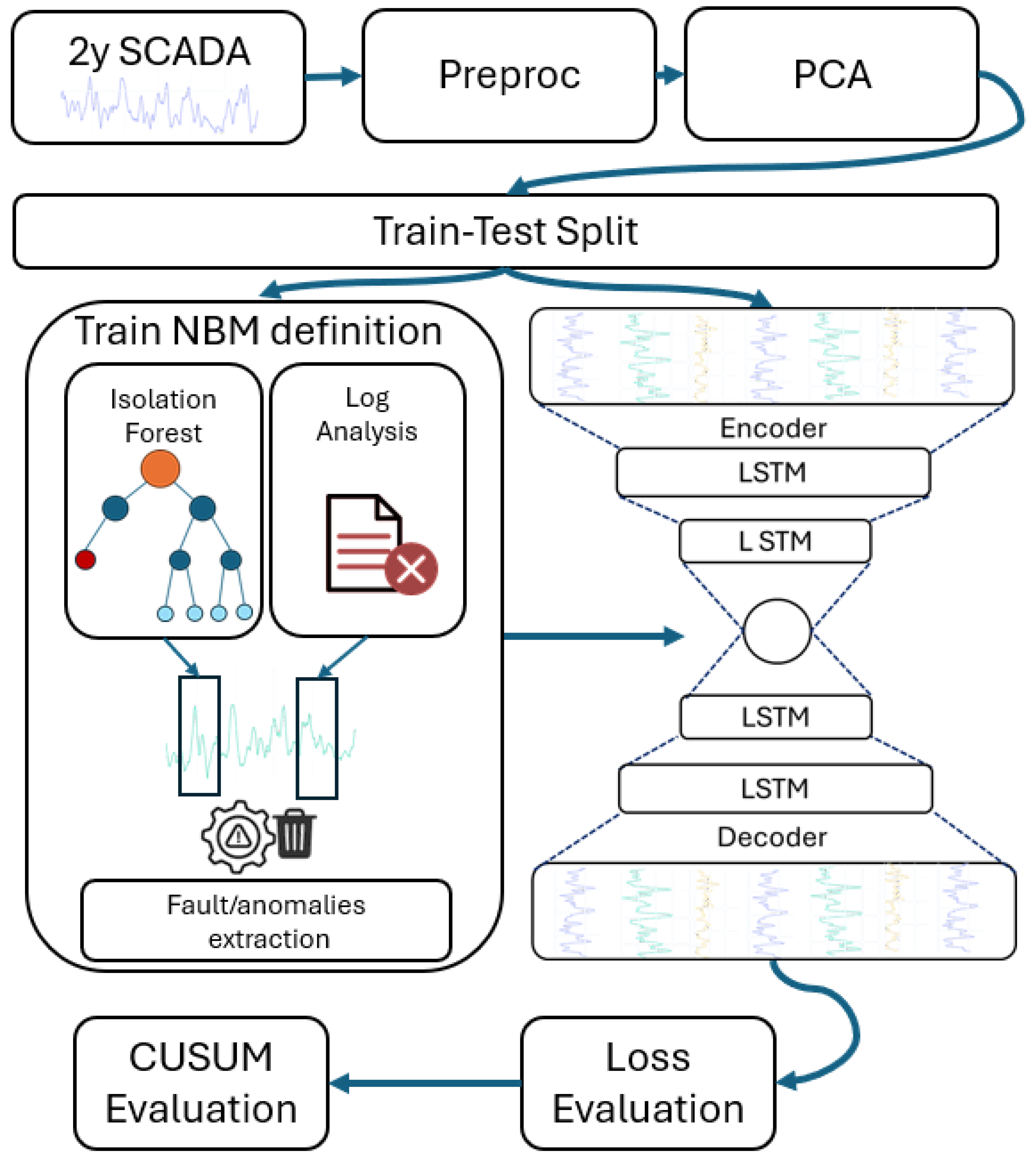
To this end, in this paper, we propose a multi-modal anomaly detection framework orchestrating an unsupervised module (i.e., decision tree method) with a supervised one (i.e., BI-LSTM AE). The proposed framework processes a dataset containing raw SCADA signals but also detailed logs of failure events and recorded alarms triggered by the SCADA system, on a wide range of subsystems: from gearbox to transformers and generators. These logs prove instrumental in validating the model’s findings and defining the reconstruction task for the autoencoder. Before being injected into the BI-LSTM AE, the SCADA data undergo a series of crucial preprocessing steps, from data cleaning to data integrity check. Next, feature engineering techniques are employed to enhance the information content of the dataset by creating new derived variables. Finally, Principal Component Analysis (PCA) is applied to reduce the dimensionality of the data, focusing on principal components that capture 98% of the total variance. In order to complement the warning log information, an unsupervised method for anomaly detection, i.e., an Isolation Forest algorithm, is in charge of labeling additional anomalies emerging from the preprocessed dataset. To perform anomaly detection, the AE is trained to learn the Normal Behavior Model (NBM) of the system. By evaluating indicators based on model reconstruction errors, the framework is able to trigger warnings. We tested the model on SCADA data gathered from one WT of an offshore wind farm located in the Guinea Gulf and covered a two-year period [32]. Results showed that the proposed model successfully predicts 21 out of 23 SCADA log alarms involving some of the most critical components, with 4 false alarms triggered.

This article is a revised version of a paper presented at the 16th European Conference on Turbomachinery Fluid dynamics & Thermodynamics, Hannover, 24–28 March 2025 [33].

The rest of the paper is organized as follows. In Section 2, we present the proposed BI-LSTM autoencoder neural architecture together with the building blocks of the deep anomaly detection framework. Then, in Section 3, we describe the case study, and in Section 4, the obtained results. Section 5 provides a final summary of conclusion.

2. Models and Methods

This section describes the deep learning-based method for anomaly detection. Specifically, Section 2.1 outlines the method used to identify periods of anomalous behavior through the unsupervised Isolation Forest algorithm, in order to subsequently train the autoencoder on a time series of wind turbine data characterized only by normal operating behavior. The architecture of the autoencoder is described in Section 2.2. Finally, Section 2.3 provides a comprehensive description of the entire pipeline, from the preprocessing of SCADA data to the actual detection of anomalies.

2.1. Isolation Forest

The Isolation Forest (IF) is an unsupervised machine learning algorithm specifically designed for anomaly detection. Unlike traditional methods that model normal data distributions to identify outliers, IF isolates anomalies by taking advantage of their unique characteristics: they are few in number and different from the majority of other data [34].

The algorithm is composed of multiple isolation trees (ITs). In these ITs, the dataset is recursively and randomly partitioned until each data point is isolated or the tree reaches its maximum height. The key assumption behind IF is that anomalous points are more likely to be isolated near the root of the tree, while points in denser regions of the feature space require more splits, resulting in a higher position within the tree.

Since each partition is generated randomly, individual trees are constructed with different sets of partitions. The path length h(x) of a point x is computed as the number of edges that it traverses when it moves from the root node to its final node (leaf) in an IT. Considering n the number of samples, h(x) is then used to compute an anomaly score s(x, n):

$$s(x,n)=2^{-{\displaystyle \frac{E\left(h\right(x\left)\right)}{c\left(n\right)}}}$$

(1)

where E(h(x)) represents the average value of h(x) across the different ITs and c(n) the expected path length for an unsuccessful search. A value of s close to 1 indicates an anomaly, while a value below 0.5 represents a normal instance. The fraction of samples that are actually considered anomalous is referred to as contamination C, and it is a parameter that defines the expected proportion of outliers within the dataset, based on the value of the anomaly score.

2.2. Autoencoder Neural Architecture

In this work, we trained an autoencoder on a dataset that is representative of the normal behavior of a turbine in order to obtain a data-driven NBM. The latter structure, composed of an encoder and a decoder, both include Bidirectional Long-Short Term Memory (BI-LSTM) layers.

LSTMs, introduced by Hochreiter et al. [35], are a type of Recurrent Neural Network (RNN) capable of capturing both long-term and short-term dependencies in time series data. They are characterized by a memory cell and three non-linear gates: an input gate $i_t$, an output gate $o_t$, and a forget gate $f_t$ (the latter proposed by Gers et al. [36]). The forward calculation process of the LSTM network at time t is defined by the following equations:

$$\begin{array}{cc}\hfill f_t& =\sigma (W_f·x_t+U_f·h_{t-1}+b_f)\hfill \end{array}$$

(2)

$$\begin{array}{cc}\hfill i_t& =\sigma (W_i·x_t+U_i·h_{t-1}+b_i)\hfill \end{array}$$

(3)

$$\begin{array}{cc}\hfill o_t& =\sigma (W_o·x_t+U_o·h_{t-1}+b_o)\hfill \end{array}$$

(4)

$$\begin{array}{cc}\hfill {\tilde{c}}_t& =tanh(W_c·x_t+U_c·h_{t-1}+b_c)\hfill \end{array}$$

(5)

$$\begin{array}{cc}\hfill c_t& =f_t\circ c_{t-1}+i_t\circ {\tilde{c}}_t\hfill \end{array}$$

(6)

$$\begin{array}{cc}\hfill h_t& =o_t\circ tanh\left(c_t\right)\hfill \end{array}$$

(7)

$$\begin{array}{cc}\hfill {\overline{h}}_t& =x_t+h_t\hfill \end{array}$$

(8)

where $W_f$, $U_f$, $b_f$, $W_i$, $U_i$, $b_i$, $W_o$, $U_o$, $b_o$, $W_c$, $U_c$, and $b_c$ are the weights of the network; $x_t$, $h_t$, $c_t$, and ${\overline{h}}_t$ are, respectively, the input, hidden state, cell state and LSTM output vector. $\sigma$ and tanh represent the sigmoid and the hyperbolic tangent activation functions.

Including information from future time steps in the input of an RNN can significantly improve the model’s performance. One possible approach, proposed by [37], consists of delaying the output by a certain number of time frames. On the one hand, increasing this delay allows the model to capture more information, but on the other, it increases the model’s effort in remembering the input information. Therefore, choosing the appropriate delay that maximizes the model’s performance is crucial and inevitably requires a “trial and error” approach, which clearly represents a limitation of this method. A different method was proposed by [38], which involves the use of Bidirectional RNNs (BiRNNs). In this architecture, the neurons of an RNN are split into two parts: one processes data in the forward direction, while the other processes them in the backward direction. This allows the model to be trained with input data coming from both past and future time steps relative to the current one. Moreover, since the two parts are entirely independent of each other, they can be trained like a regular unidirectional RNN by unrolling them into a general feedforward network. In this work, we chose to use bidirectional LSTM layers within the autoencoder. Building on the discussion of generic bidirectional networks and LSTMs, it is possible to extend the formulation presented in equations from (2) to (8) to the case of a forward ($\overrightarrow{\mathrm{LSTM}}$) and a backward ($\overleftarrow{\mathrm{LSTM}}$) network.

The autoencoder is a type of neural network that learns to transform input data into a latent representation [39], then reconstructs it back to its original form, making it well-suited for anomaly detection tasks [40]. In fact, by learning the typical patterns in turbine operation, the autoencoder can highlight deviations from the normal behavior when abnormal conditions arise. The structure of the autoencoder consists of two main components: the encoder and the decoder. The encoder’s role is to learn a different-dimensional representation of the input data by capturing temporal dependencies and key features in the data. Once the data has been transformed by the encoder, the decoder attempts to reconstruct the original input. In fact, the decoder starts by repeating the encoded sequence using a repeat vector layer to match the original sequence length. Then, the BI-LSTM layers are employed mirroring the structure of the encoder. Finally, the output is passed through a time-distributed dense layer with a ReLU activation function, which processes each time step individually to generate the reconstructed input. The loss is defined as the Mean Absolute Error (MAE) between the original input sequence and the reconstructed sequence, calculated as follows:

$$L(x^{\prime },x)=\parallel x^{\prime }-x\parallel$$

(9)

where x represents the original input and $x^{\prime }$ the reconstructed sequence. The autoencoder is trained using the Adam optimizer, with a total of E epochs, and early stopping is employed to prevent overfitting.

2.3. Detection Framework

In this section, the proposed framework for anomaly detection in SCADA systems is presented as illustrated in Figure 1.

The proposed framework involves preprocessing the original SCADA dataset as the first step. A subset of variables is selected from the SCADA system that retains the informative content of the signal while eliminating redundant information. Then, signals presenting high levels of noise are smoothed using the Savitzky–Golay filter [41]. Moreover, considering that data are often available for limited periods of a few years, it is decided to subtract the ambient temperature from all temperature features collected from the sensors (including temperatures on the drivetrain components and in the nacelle of turbines) in order to eliminate the obvious seasonality of the signals. Subsequently, the features are scaled using MinMax Scaler, and the strong dependence of operational variables (i.e., power, rotational speed, or driving-train-related temperatures) on wind speed is neutralized in a similar way to temperature signals. In order to counterbalance the reduced amount of training data, the dimensionality of the input is reduced with the Principal Component Analysis (PCA). PCA generates a set of linearly independent dimensions, each obtained as a linear combination of the original dataset’s features [42].

To train the autoencoder, only a portion of the original dataset is selected so that during inference, the model would be exposed to the whole dataset containing data not included in the training set. Since the autoencoder’s functionality relies on its ability to extract the salient features of normal operating conditions, the training dataset is cleaned by removing the samples characterized by abnormal operating conditions. This is achieved by eliminating the time intervals surrounding the SCADA alarms recorded by the operator and by removing anomalous data identified through the unsupervised Isolation Forest approach.

Once the autoencoder has been trained on the training data, it is then exposed to the complete dataset, which includes both anomalous events and the portion of the dataset that had initially been excluded. During inference, the loss, as defined in expression (9), is evaluated, and events are considered anomalous when their loss values exceed a threshold set at the 90th percentile of the loss distribution. Moreover, to assess both the persistence and severity of an anomaly, a control chart is employed as defined in the following expression:

$$CUSU{M}_i=max\left(0,CUSU{M}_{i-1}+L_i-\mathrm{T}\right)$$

(10)

where $L_i$ represents the loss at the i-th timestamp and T is a threshold set at two-thirds of the value of the 90th percentile of the loss. In fact, by cumulatively assessing deviations in the loss over time, CUSUM provides insights into whether an anomaly represents a short-lived fluctuation or a more sustained deviation from the norm. This enables a more comprehensive understanding of the anomalous behavior, complementing the initial loss-based detection.

Performance is evaluated using classic error metrics such as Mean Absolute Error (MAE), Mean Squared Error (MSE), and Root Mean Squared Error (RMSE). Furthermore, True Positives (TPs) are defined as model warnings that are followed by an event within the next time window, consisting of $T_f=4320$ samples (1 month); False Positives (FPs) as warnings that are not followed by any event; and False Negatives (FNs) as events that are not preceded by any warnings. Moreover, the typical classification metrics, as described in the following expressions, are also considered:

$$Precision\left(P\right)={\displaystyle \frac{TP}{TP+FP}}$$

(11)

$$Recall\left(R\right)={\displaystyle \frac{TP}{TP+FN}}$$

(12)

$$F-1Score\left(F1\right)=2·{\displaystyle \frac{P·R}{P+R}}$$

(13)

Moreover, although the use of these metrics represents the standard for evaluating the performance of classification models [43], they lack a quantification of the operational impact that such performance has on the use of an anomaly detection system. Therefore, it becomes necessary to estimate both the savings resulting from early fault detection and the costs associated with false alarms and missed fault detections. Since this estimation is heavily influenced by site-specific factors, the literature lacks established methods. However, for the open data set EDP [32], the following method is introduced by [44]. In particular, savings for each detection are quantified as

$$T{P}_s=\sum _{i=1}^{n_{TP}}\left(Cos{t}_{rpl}-\left(Cos{t}_{rpr}+(Cos{t}_{rpl}-Cos{t}_{rpr})\left(1-{\displaystyle \frac{\mathrm{\Delta }t}{60}}\right)\right)\right)$$

(14)

where $n_{TP}$ is the number of TP; $Cos{t}_{rpl}$ and $Cos{t}_{rpr}$ are, respectively, the costs of replacing and repairing a specific component; and $\mathrm{\Delta }t$ is the time from the alarm to the event. Meanwhile, costs related to the missed detection of a fault are given by

$$F{N}_c=n_{FN}\times Cos{t}_{rpl}$$

(15)

where $n_{FN}$ is the number of FN. Finally, costs related to unnecessary inspections caused by false alarms are quantified by

$$F{P}_c=n_{FP}\times Cos{t}_{insp}$$

(16)

where $n_{FP}$ is the number of FP, and $Cos{t}_{insp}$ represents the costs of inspections. In addition, for the open dataset EDP, $C_{rpr}$ and $C_{rpl}$ are also listed for the different components of turbines [44]. Finally, Total Prediction Savings are defined by

$$TPS=T{P}_s-F{N}_c-F{P}_c$$

(17)

3. Case Study

Data are derived from one turbine of an offshore wind farm located in the Guinea Gulf and cover the period from January 2016 to December 2017. The turbine considered, ranked class 2 according to the standard IEC 61400 [45], is bottom-fixed, with a rotor diameter of 90 m, maximum rotor speed 14.9 rpm, and 2 MW rated power at a nominal wind speed of 12 m/s.

Table 1. WT technical specifications.

EDP Wind Turbines Main Features	Value
Rated power (kW)	2000
Cut-in wind speed (m/s)	4
Rated wind speed (m/s)	12
Cut-out wind speed (m/s)	25
Hub height (m)	80
Number of blades	3
Rotor diameter (m)	90
Rotor swept area (m2)	6362
Max rotor speed (rpm)	14.9
Max rotor tip speed (m/s)	70
Rotor power density 1 (W/m2)	314.4
Rotor power density 2 (m2/kW)	3.2
Gearbox type	Planetary/spur
Gearbox stages	3
Generator type	Asynchronous
Max generator speed (rpm)	2016
Generator voltage (V)	690
Grid frequency (Hz)	50

summarizes the technical specifications of wind turbine under scrutiny.

Data recording and visualization are made possible by a dense network of sensors located along the nacelle of the wind generator. Sensors for wind speed, wind direction, shaft rotation speed, and numerous other factors collect and transfer data to the PLC (Programmable Logic Controller) to enable real-time operators’ control on the generation profile. WTs are equipped with a SCADA system for the monitoring of multiple parameters collected from the main components together with ambient measurements that are recorded every 10 min in terms of the mean, minimum value, maximum value and standard deviation. From the complete dataset, which includes 84 features, 30 signals have been selected as listed in

Table 2. Features selected from WT SCADA system.

Description	Component
Temp. gen. bearing 1 (NDE)	Generator Bearings
Temp. gen. bearing 2 (DE)	Generator Bearings
Gen. rpm	Generator
Temp. gen. phase L1	Generator
Temp. gen. phase L2	Generator
Temp. gen. phase L3	Generator
Temp. slipring	Generator
Temp. hydraulic oil	Hydraulic
Temp. gearbox oil	Gearbox
Temp. gearbox bearing at HSS	Gearbox
Temp. nacelle	Nacelle
Nacelle direction	Nacelle
Rotor rpm	Rotor
Wind speed	Ambient
Wind relative direction	Ambient
Wind absolute direction	Ambient
Ambient temperature	Ambient
Total active power	Production
Total reactive power	Production
Grid Power Request	Grid
Temp. HV transf. phase L1	Transformer
Temp. HV transf. phase L2	Transformer
Temp. HV transf. phase L3	Transformer
Temp. the top nacelle controller	Controller
Temp. the hub controller	Controller
Temp. VCP-board	Controller
Temp. choke coils at VCS-section	Controller
Temp. VCS cooling water	Controller
Temp. nose cone	Spinner
Blades pitch angle	Blades

. The features excluded from the analysis are the minima, maxima, and standard deviations of the original features, along with most grid-related variables (such as frequency and reactive power on the grid side) and the active and reactive power for each phase of the generator. In the table, “Temp.” is short for ”temperature“, and “gen.” abbreviates “generator”, while “trans.” stands for “transformer”. When referring to bearing locations, two bearings are monitored at the generator: one at the drive end (DE) and one at the non-drive end (NDE). At the gearbox, a bearing is monitored at the high speed shaft (HSS).

Datasets are completed with event logs recording the list of alarms during the period of interest as summarized in

Table 3. Fault and warning logs.

ID	Date	Description
L1	3 July 2016 16:29	Hot HV trafo
L2	25 July 2016 12:41	Hot HV trafo
L3	6 August 2016 12:29	High temperature
L4	4 September 2016 12:42	Hot HV trafo
L5	29 October 2016 11:00	High temperature
L6	26 January 2017 22:00	Thermoerror yaw motor
L7	20 April 2017 03:50	High windspeed
L8	20 April 2017 23:42	High windspeed
L9	11 June 2017 16:18	Hot HV trafo
L10	16 June 2017 22:07	Oil leakage in hub
L11	20 June 2017 15:26	Hot HV trafo
L12	4 July 2017 09:04	Oil leakage in hub
L13	20 August 2017 12:56	Oil leakage in hub
L14	21 August 2017 09:00	Oil leakage in hub
L15	19 October 2017 09:22	Oil leakage in hub
F1	10 July 2016 03:46	High temperature transformer
F2	23 August 2016 02:21	High temperature transformer (Transformer refrigeration repaired)
F3	20 August 2017 06:08	Generator bearings damaged
F4	21 August 2017 14:47	Generator damaged
F5	17 June 2017 11:35	Oil leakage in hub
F6	19 October 2017 10:11	Oil leakage in hub

. The lists counting 21 events include all the events considered in the present anomaly detection study. These are obtained from the list of failure events made available by the files “Historical-Failure-Logbook-2016” and “opendata-wind-failures-2017” (denoted by the letter F in the table) and from the event log (denoted by the letter L in the table) contained in the files “Wind-Turbines-Logs-2016” and “Wind-Turbines-Logs-2017”, which includes all events recorded by the SCADA system on the wind turbine during the reported period [32]. Following Reliawind turbine taxonomy [46], the event log includes anomalies categorized at assembly and sub-assembly levels but only a few alarms at the component/part level. In addition, we filtered out all false alarms and minor events not leading to repair or replacement actions. When looking closely at the alarm logs, it is noticeable that the majority of events relate to WT drive train and electric sub-systems. In particular, the turbine had seven alarms relating to high temperature of the transformer (10 July and 23 August 2016) and a major failure of the generator on 21 August 2017.

For model training, the portion of the dataset spanning from January 2016 to June 2017 is used. Moreover, periods surrounding anomalies detected through Isolation Forests and recorded failures are removed from the training dataset. Specifically, for anomalies detected through IF, the 24 h preceding and following each event are excluded. For failures, the 24 h preceding and 72 h following each failure are also excluded.

4. Results

4.1. Deep Learning Detection Settings

As explained in Section 3, the dataset consisting of the 30 features shown in Table 2 is preprocessed and subsequently reduced using PCA. In particular, the Savitzky–Golay is applied using a window length of 24 time steps (corresponding to 4 h) and a third-order polynomial to fit the samples. As an example, Figure 2 shows the signal related to the hydraulic oil average temperature in the period from 1 January to 2 January 2017, for both the unfiltered signal (blue line) and the filtered signal (red line).

In the application of PCA, we chose to capture 98% of the variance, which results in a new feature space characterized by 11 principal components. Moreover, using the Isolation Forest algorithm with a contamination rate of 0.001, 73 anomalous periods are removed from the training dataset.

The autoencoder model consists of a bidirectional LSTM-based encoder–decoder architecture. The encoder consists of a Bi-LSTM layer; the first has a dimension of 128, while the second, of 64. The decoder reconstructs the input sequence from this latent representation using a mirrored dimensions layer. The Adam optimizer is employed with a learning rate of 0.0001. The model is trained for a maximum of 100 epochs, with early stopping applied to prevent overfitting, based on validation loss with a patience of 5 epochs.

4.2. Anomaly Detection

In this section, the results obtained during the model’s inference phase are presented. Specifically, Figure 3 shows the reconstruction loss and the threshold value set at the 90th percentile for the whole test period. The choice of this threshold value has been subject to a sensitivity analysis, which is discussed later in this section. The figure highlights failure events with solid lines. Loss spikes that exceed the threshold trigger an alarm and are considered precursors to failure.

Figure 4, Figure 5, Figure 6 and Figure 7 provide a detailed overview of the periods characterized by faults and loss peaks, also highlighting the events from the log (dashed lines). The areas highlighted in yellow represent the intervals between the events that precede and follow each failure event. In Figure 4, fault F1 labeled as “High temperature transformer” is shown, preceded and followed by two high-temperature readings, both occurring at the transformer. In this case, the proposed method is able to detect the onset of the fault 13 days in advance. Similarly, Figure 5 highlights fault F2, which is of the same nature as F1. It is likewise preceded and followed by high-temperature recordings at the transformer, with reconstruction loss spikes detected in advance of the fault. Given the nature of the logs (from L1 to L5), it becomes evident that the loss above the threshold signals the tail of phenomena related to high-temperature conditions that are not necessarily correlated with severe operational stress. Figure 6 shows two peaks in the reconstruction loss that are not related to the onset of faults but to two anomalous operating conditions. Specifically, the first peak occurs in correspondence with the “Thermoerror way motor” signal and is linked to the inability of the turbine to properly align with the wind due to the correct functioning of the yaw regulation. The second peak, on the other hand, corresponds to two “High windspeed” alerts and is therefore representative of the unusual environmental conditions for the turbine. Finally, Figure 7 illustrates the period encompassing faults F3, F4, F5, and F6. The first (F3) is a fault in the generator bearings, which likely led to the subsequent generator failure (F4), while F5 and F6 are attributed to oil leaks. All faults, except F6, are preceded by alarm signals, and the reconstruction loss demonstrates high sensitivity to this sequence of events as evidenced by the spike in values. Moreover, considering the nature of the logs from L9 to L15—all of which are related to oil leaks, except for L9 and L11 which correspond to high-temperature readings—it can be inferred that these anomalies are more closely linked to oil leakage and gear damage, rather than being solely attributable to high-temperature conditions.

Figure 8 and Figure 9 show the progression of the CUSUM, highlighting the same areas identified by the spikes in the reconstruction loss. Specifically, Figure 8 emphasizes the regions where the CUSUM remains elevated even after the fault, corresponding to the zones depicted in Figure 4 and Figure 5 (combined into event chain A), and in Figure 7 (event chain B). In both cases, it is clear that the CUSUM not only confirms the observations made by the loss but also provides additional information on the persistence, and therefore the severity, of the anomaly. Conversely, in Figure 9, two CUSUM peaks are highlighted, corresponding to the two peaks in the loss shown in Figure 6, which are not related to fault phenomena but rather to anomalous operating conditions.

Considering both the log and fault events in the count of TPs, FPs, and FNs, the metrics defined in Section 2.3 are calculated.

Table 4. Performance summary for BI-LSTM autoencoder.

Metric	Value
Mean Absolute Error (MAE)	0.0536
Mean Square Error (MSE)	0.0051
Root Mean Square Error (RMSE)	0.0679
False Positives (FP)	4
True Positives (TP)	12
False Negatives (FN)	2
Precision	0.75
Recall	0.86
F1 Score	0.8

reports the values of these metrics as well as the count of TPs, FPs, and FNs.

Furthermore,

Table 5. Threshold sensitivity analysis.

Percentile	TP	FP	FN	P	R	F1
80°	12	12	2	0.50	0.86	0.63
85°	12	9	2	0.57	0.86	0.65
90°	12	4	2	0.75	0.86	0.80
95°	5	1	10	0.83	0.33	0.48

presents the values of these metrics as the alarm threshold varies. Specifically, the threshold is set at the 80th, 85th, 90th, and 95th percentiles of the reconstruction loss. For thresholds lower than the 90th percentile, a higher number of FP is observed, while the number of FN remains unchanged. This leads to a decrease in precision and, consequently, in the F1 Score. On the other hand, setting the threshold above the 90th percentile increases precision at the expense of the method’s ability to detect failure events. In particular, when the threshold is set at the 95th percentile, the number of FN increases to 10, resulting in lower recall and F1 Score compared to the case where the threshold is set at the 90th percentile.

Moreover, considering the discussion presented in Section 2.3, the obtained TPS are equal to EUR 190.7 k. In particular, TPs are equal to EUR 209.1 k, $F{P}_c$ to EUR 14.4 k and $F{N}_c$ to EUR 4 k.

Table 6. Anomaly detection results.

ID	Date	Class
A1	27 June 2016 15:10	TP
A2	9 July 2016 22:30	TP
A3	11 August 2016 22:50	TP
A4	1 September 2016 17:40	TP
A5	14 September 2016 22:00	FP
A6	19 September 2016 11:40	FP
A7	29 September 2016 08:20	TP
A8	25 January 2017 17:30	TP
A9	19 April 2017 11:40	TP
A10	21 April 2017 09:50	FP
A11	11 June 2017 06:40	TP
A12	14 June 2017 03:40	TP
A13	11 July 2017 11:20	FP
A14	4 August 2017 15:10	TP
A15	13 August 2017 19:10	TP
A16	19 August 2017 13:30	TP
L15	19 October 2017 09:20	FN
F6	19 October 2017 10:10	FN

presents the triggered alarms (from A1 to A16) classified either as TP or FP, together with the two missed events L15 and F6, classified as FN. Consecutive TPs (i.e., TPs that are anticipating the same event) are counted as one.

Table 7. Model performance comparison.

Model	MAE	MSE	RMSE
BI_LSTM	0.0536	0.0051	0.0679
MTGCAE	0.0380	0.0040	0.0610
LSTM_AE	0.0530	0.0070	0.0850
CNN_LSTM	0.0510	0.0070	0.0820

presents a comparison of the BI-LSTM AE performance against some alternative models for anomaly detection. The performance of the models was previously calculated in [40] in terms of MAE, MSE, and RMSE, using data from the entire wind farm within the same dataset.The proposed model is showing reduced error when compared with LSTM and CNN_LSTM AEs, while still underperforming with respect to more complex models such as a Multivariate Timeseries Graph Convolutional AutoEncoder (MTGCAE; introduced in [40]).

5. Conclusions

The present work proposes a semi-supervised anomaly detection framework for horizontal axis wind turbines, based on artificial intelligence techniques applied to SCADA data. Specifically, real-world open data provided by EDP Renewables, collected from offshore wind turbines operating in the Gulf of Guinea, are used. In addition to SCADA data covering two years of operations of a single turbine, event and failure logs, also made available in open format, are considered.

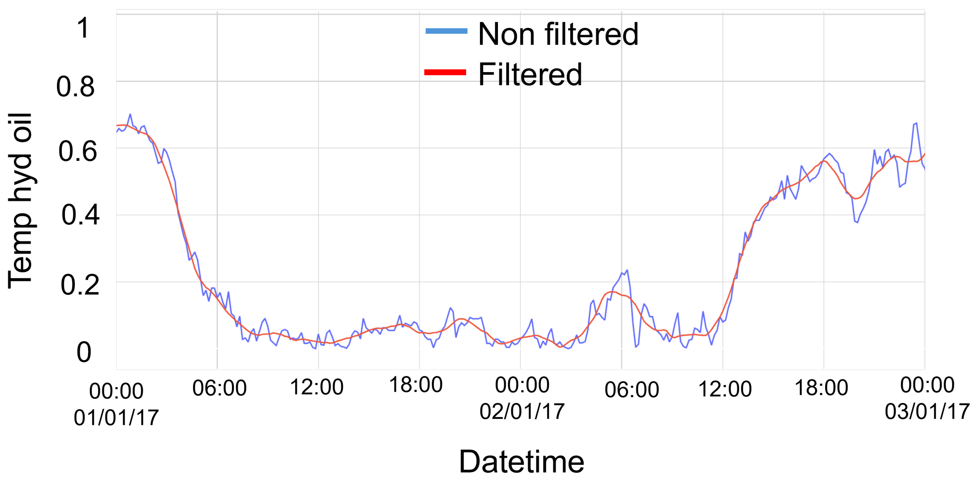
The first step of the work consists of the preprocessing of the SCADA data. Specifically, a subset of 30 significant variables is selected. The Savitzky–Golay filter is applied in order to smooth the time series data and reduce noise. The ambient temperature value is subtracted from all temperature signals to eliminate the strong seasonal trend in the data. After scaling the data using MinMax Scaling, the strong dependency of the operational variables from the wind speed (e.g., power-, rotational speed-, or drive-train-related temperatures) is neutralized in a similar fashion. From the resulting dataset, the first 70% is selected as the training dataset so that, during inference, the model would be exposed to data different from those on which it is trained.

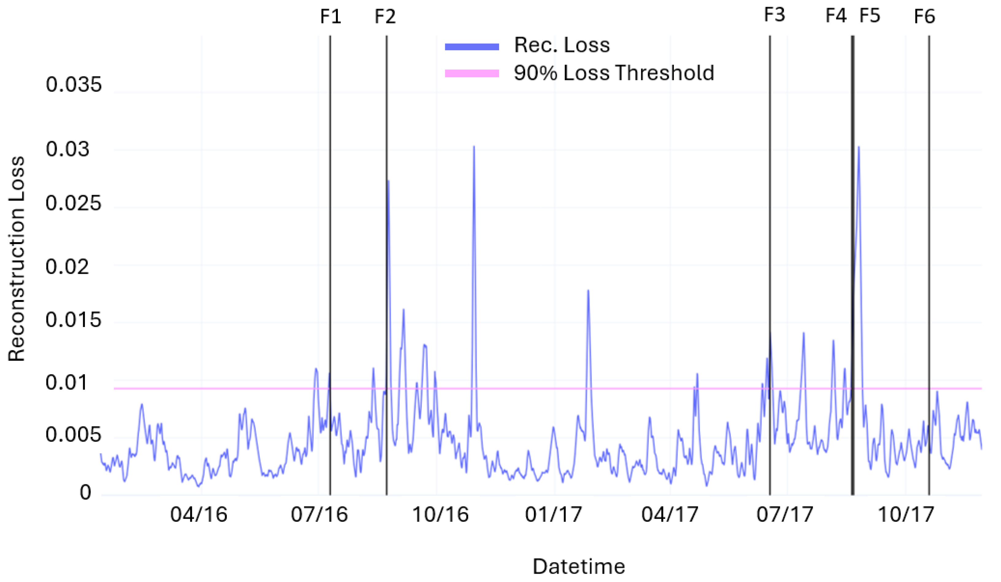
The reconstruction loss obtained from an autoencoder based on Bidirectional Long Short-Term Memory (BI-LSTM) cells is chosen as the alarm signal. Considering the need to train the autoencoder on a time series characterized by the normal behavior of the wind turbine, any interval between the 24 h prior to and the 72 h following each failure event is removed from the training dataset. Moreover, the unsupervised Isolation Forest method is used to eliminate additional anomalous operating points from the training data. Thus, with a contamination rate set at 0.001, intervals between the 24 h before and after each anomaly are removed. The resulting dataset is then used to train the autoencoder. The architecture of the autoencoder consists of an encoder made up of a BI-LSTM cell layer that transforms the input data into a latent space of 128 dimensions, and a decoder that reconstructs the input sequence from this latent representation.

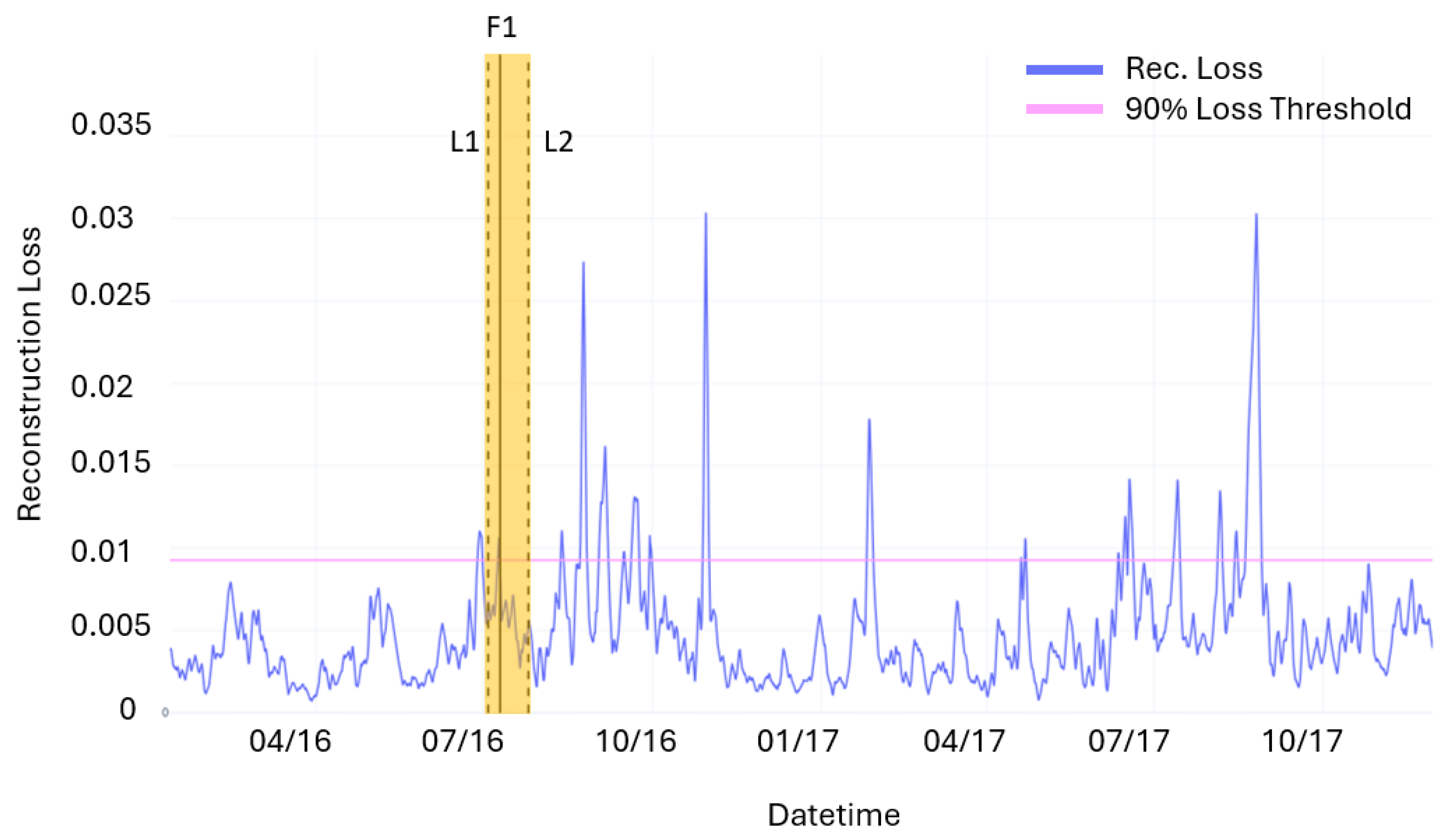
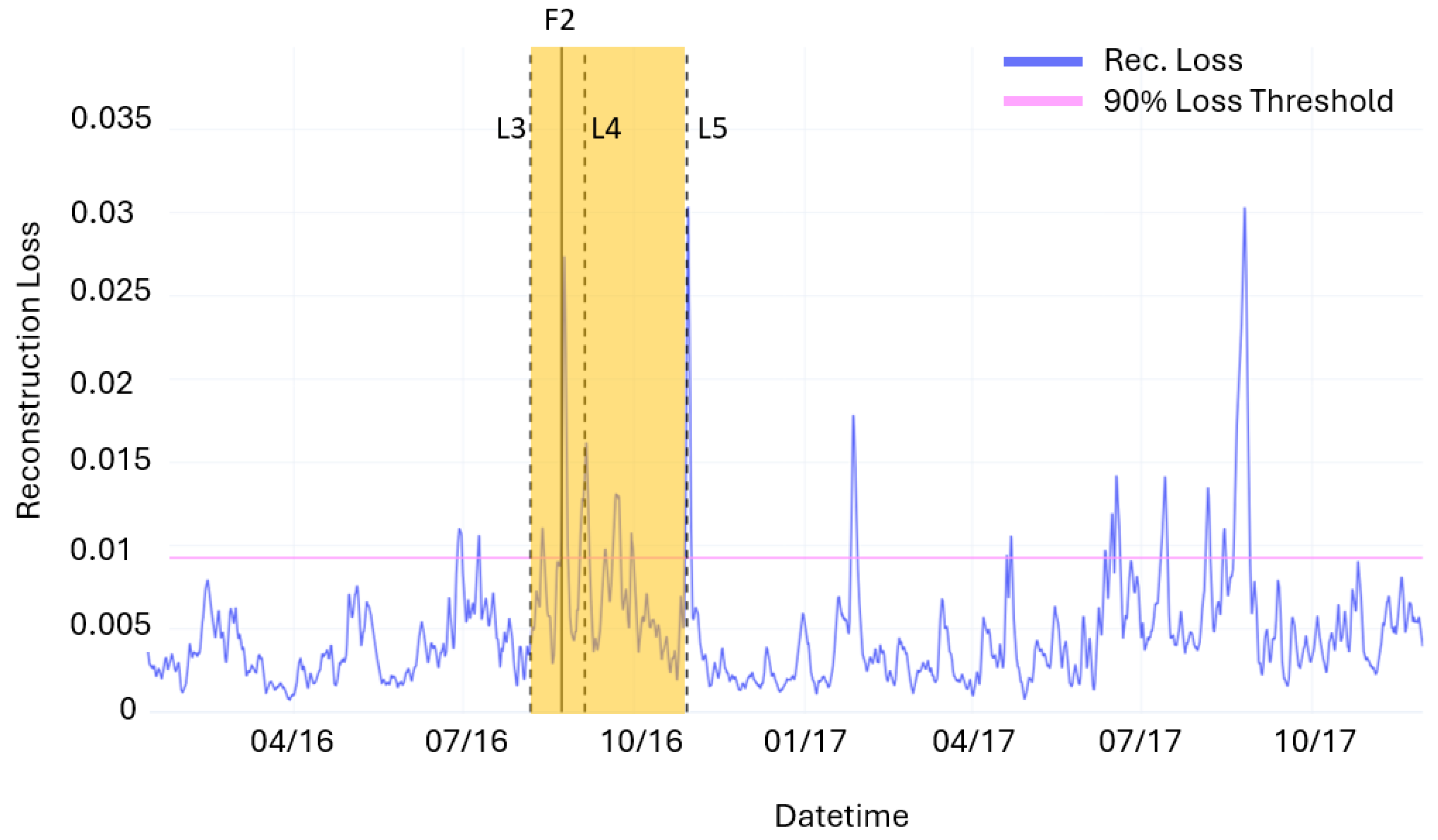
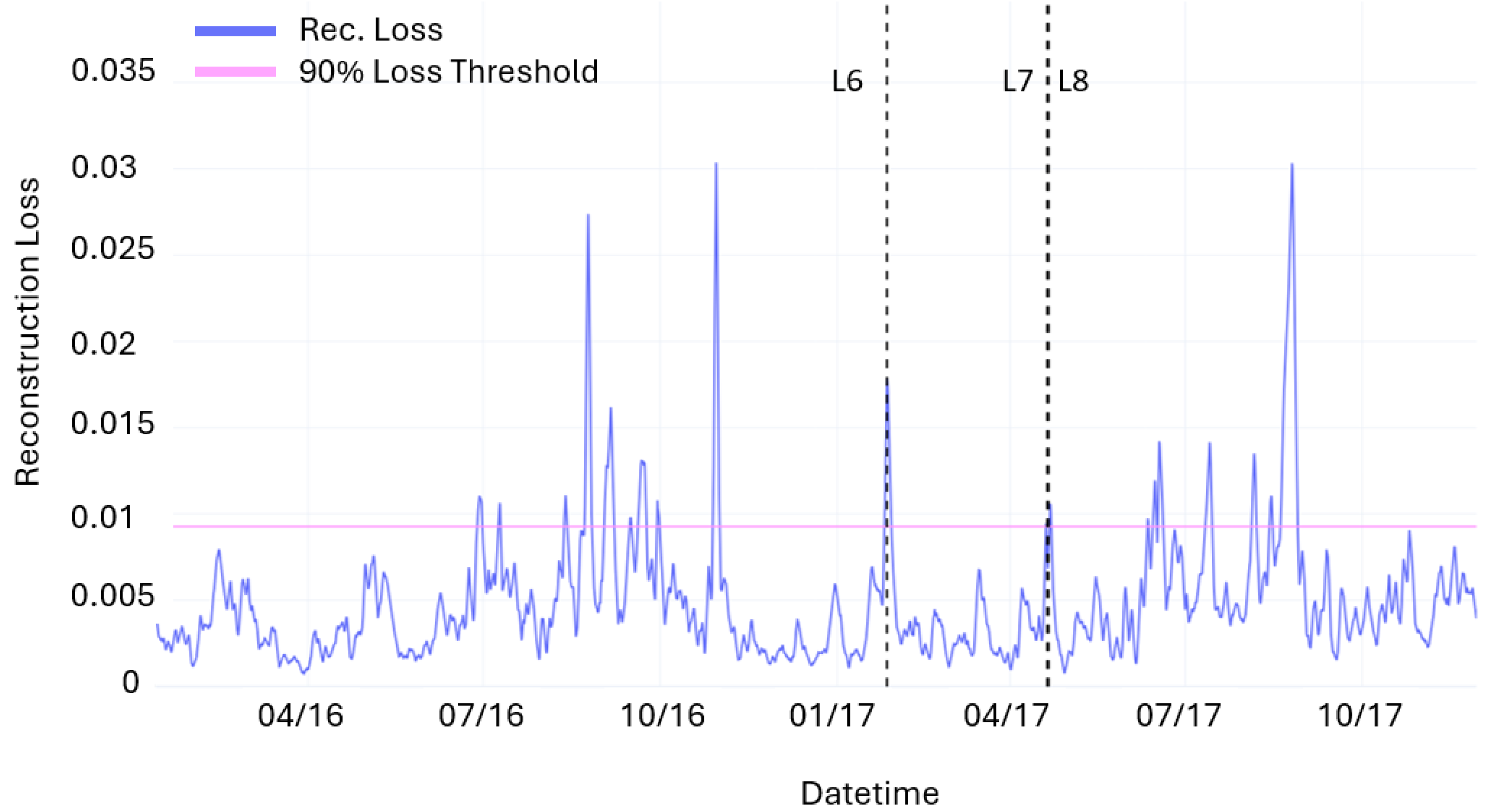
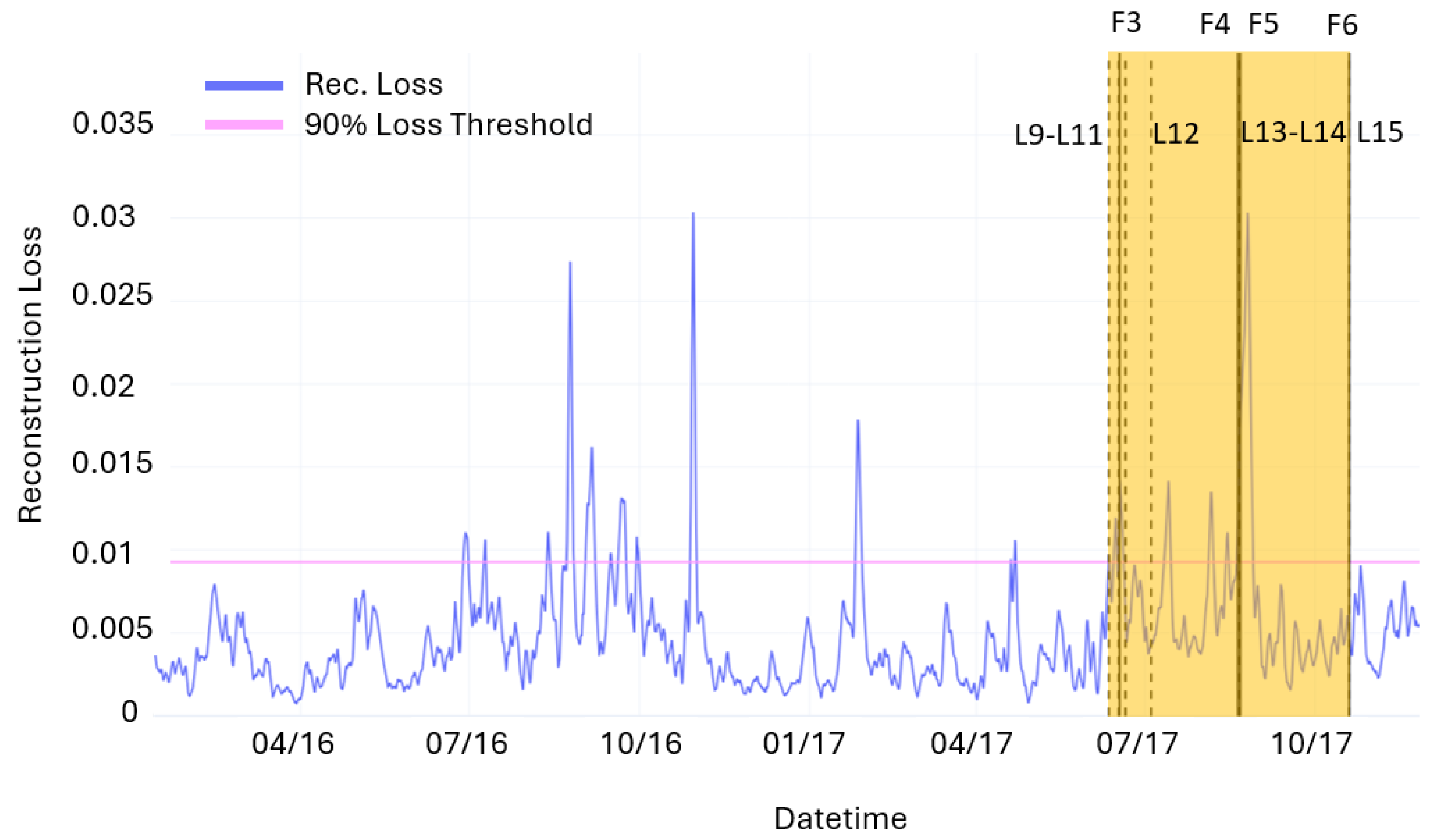
During the inference phase, the entire dataset, including the two years of turbine operations and the anomalous points identified by the failure logs and Isolation Forest, is used. Spikes in the reconstruction loss are used to trigger fault alarms. Specifically, an alarm threshold is set at the 90th percentile of the reconstruction loss value. Considering a time window ($T_f$) of 4320 samples (1 month) the predicted faults are defined as follows:

• True Positive (TP): a model warning trigger that is followed by an event within $T_f$;
• False Positive (FP): a model warning trigger that is not followed by an event within $T_f$;
• False Negative (FN): an event that is not preceded by any warnings.

In this way, 4 FPs, 12 TPs, and 2 FNs are obtained. The model’s performance is therefore expressed through the well-known metrics of precision (P), recall (R), and F1 Score (F1). The following values are obtained: P = 0.75, R = 0.86, and F1 = 0.8.

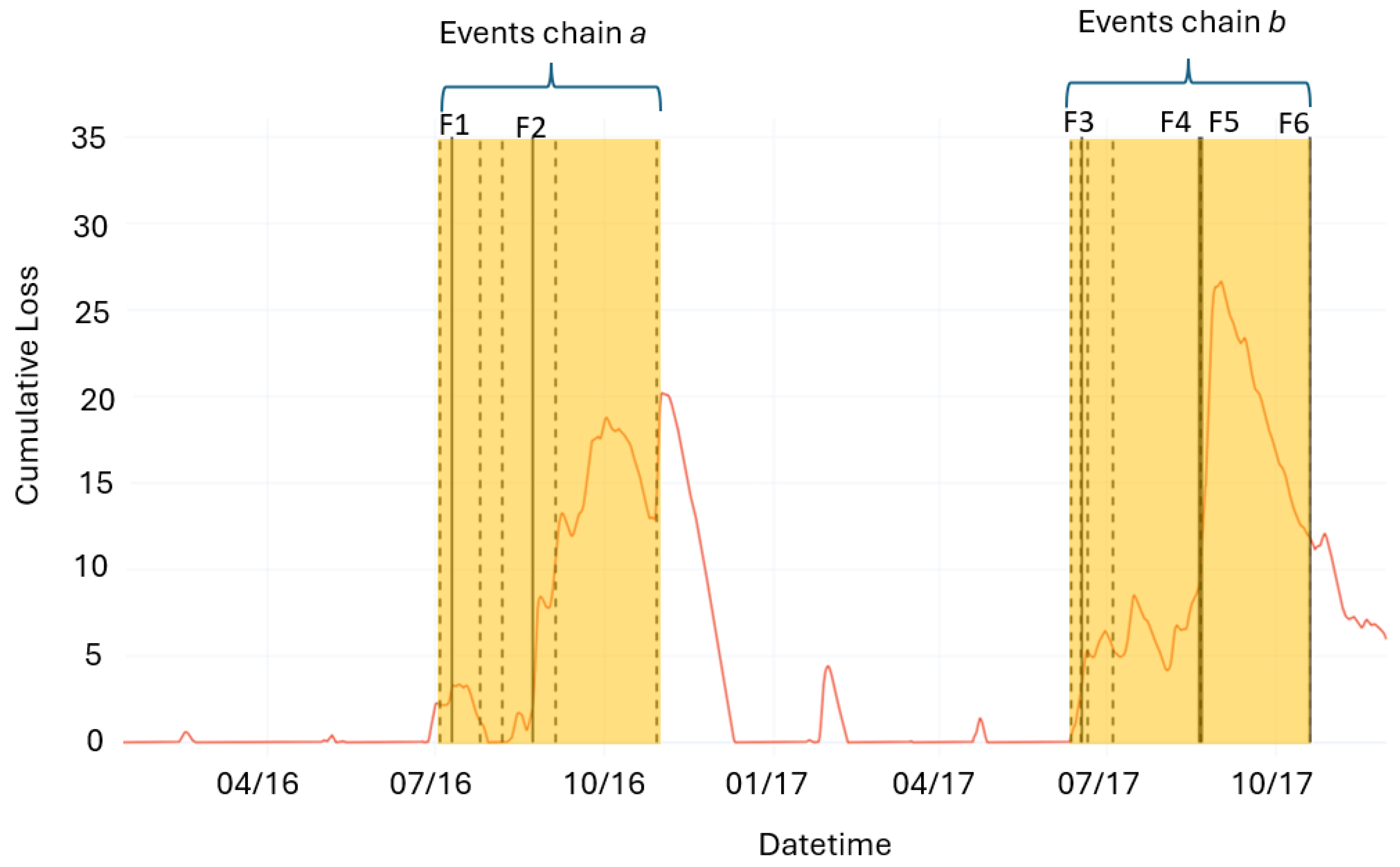
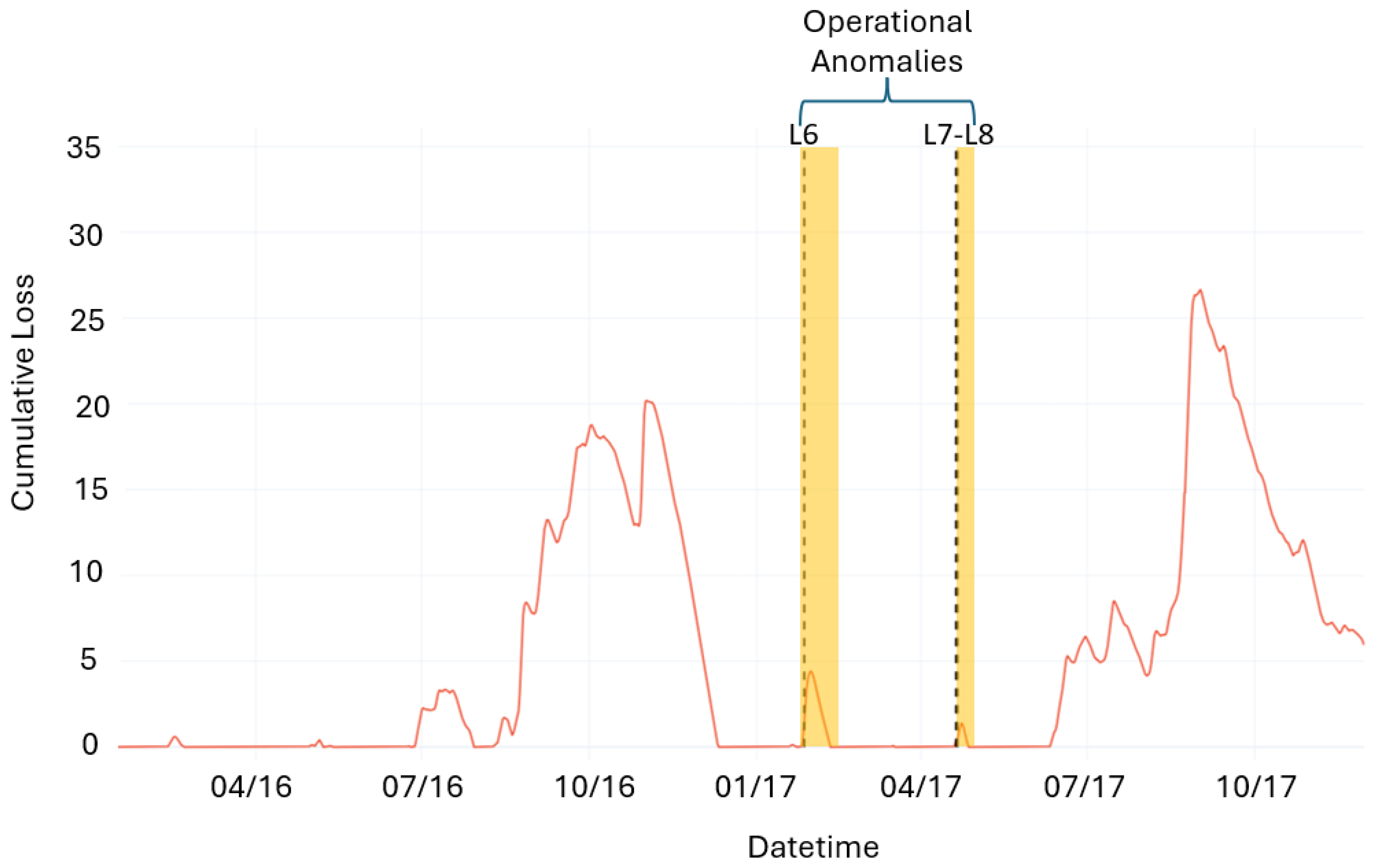
Moreover, considering only the reconstruction loss does not provide a measure of the persistence and, therefore, the severity of the anomalies. In order to obtain a better understanding of each alarm triggered by the loss, a CUSUM control chart based on the loss is used. This approach made it possible to identify two fault chains corresponding to periods where the CUSUM values remain persistently above 0. Conversely, two operational anomalies are identified where, despite the presence of loss spikes, the CUSUM value returned to 0 immediately after the event. In these cases, the reconstruction errors of the time series are not attributed to the onset of faults but rather to the occurrence of momentary anomalous operating conditions.

References

1. Liserre, M.; Cardenas, R.; Molinas, M.; Rodriguez, J. Overview of multi-MW wind turbines and wind parks. IEEE Trans. Ind. Electron. 2011, 58, 1081–1095. [Google Scholar] [CrossRef]
2. Fung, K.; Scheffler, R.; Stolpe, J. Wind energy—A utility perspective. IEEE Trans. Power Appar. Syst. 1981, PAS-100, 1176–1182. [Google Scholar]
3. Sesto, E.; Casale, C. Exploitation of wind as an energy source to meet the world’s electricity demand. J. Wind. Eng. Ind. Aerodyn. 1998, 74, 375–387. [Google Scholar] [CrossRef]
4. Wee, H.M.; Yang, W.H.; Chou, C.W.; Padilan, M.V. Renewable energy supply chains, performance, application barriers, and strategies for further development. Renew. Sustain. Energy Rev. 2012, 16, 5451–5465. [Google Scholar] [CrossRef]
5. Jain, P.; Wijayatunga, P. Grid Integration of Wind Power: Best Practices for Emerging Wind Markets, Sustainable Development; Working Paper Series, No. 43; Asian Development Bank: Mandaluyong City, Philippines, 2016. [Google Scholar]
6. Barnabei, V.F.; Ancora, T.; Conti, M.; Castorrini, A.; Delibra, G.; Corsini, A.; Rispoli, F. A Multi-Objective Optimization Framework for Offshore Wind Farm Design in Deep Water Seas. J. Fluids Eng. 2025, 147. [Google Scholar] [CrossRef]
7. Castorrini, A.; Barnabei, V.F.; Domenech, L.; Šakalyté, A.; Sánchez, F.; Campobasso, M.S. Impact of meteorological data factors and material characterization method on the predictions of leading edge erosion of wind turbine blades. Renew. Energy 2024, 227, 120549. [Google Scholar] [CrossRef]
8. Barnabei, V.; Morvillo, E.; Corsini, A.; Bonacina, F. A Systematic Study on the Use of Machine Learnt Feature Derivation in Horizontal Axis Wind Turbine Fleets. In Proceedings of the Offshore Mediterranean Conference and Exhibition, Ravenna, Italy, 23–25 May 2023; p. OMC-2023. [Google Scholar]
9. Barnabei, V.F.; De Girolamo, F.; Ancora, T.C.; Tieghi, L.; Delibra, G.; Corsini, A. Normal Behaviour Modeling of HAWT fleets using SCADA-based feature engineering. In Proceedings of the GPPS2024 Chania, Global Power and Propolsion Society Technical Conference, Chania, Greece, 4–6 September 2024. [Google Scholar] [CrossRef]
10. Kim, K.; Parthasarathy, G.; Uluyol, O.; Foslien, W.; Sheng, S.; Fleming, P. Use of SCADA data for failure detection in wind turbines. In Proceedings of the Energy Sustainability, Washington, DC, USA, 7–10 August 2011; Volume 54686, pp. 2071–2079. [Google Scholar]
11. Dao, C.; Kazemtabrizi, B.; Crabtree, C. Wind turbine reliability data review and impacts on levelised cost of energy. Wind Energy 2019, 22, 1848–1871. [Google Scholar] [CrossRef]
12. Wen, X.; Xie, M. Performance evaluation of wind turbines based on SCADA data, Wind Engineering, SAGE Journals 2021. Wind Eng. 2021, 45, 1243–1255. [Google Scholar] [CrossRef]
13. Stetco, A.; Dinmohammadi, F.; Zhao, X.; Robu, V.; Flynn, D.; Barnes, M.; Keane, J.; Nenadic, G. Machine learning methods for wind turbine condition monitoring: A review. Renew. Energy 2019, 133, 620–635. [Google Scholar] [CrossRef]
14. Maldonado-Correa, J.; Martín-Martínez, S.; Artigao, E.; Gómez-Lázaro, E. Using SCADA data for wind turbine condition monitoring: A systematic literature review. Energies 2020, 13, 3132. [Google Scholar] [CrossRef]
15. Cui, Y.; Bangalore, P.; Bertling Tjernberg, L. A fault detection framework using recurrent neural networks for condition monitoring of wind turbines. Wind Energy 2021, 24, 1249–1262. [Google Scholar] [CrossRef]
16. Ibrahim, H.; Ghandour, M.; Dimitrova, M.; Ilinca, A.; Perron, J. Integration of Wind Energy into Electricity Systems: Technical Challenges and Actual Solutions. Energy Procedia 2011, 6, 815–824. [Google Scholar] [CrossRef]
17. Chen, H.; Xie, C.; Dai, J.; Cen, E.; Li, J. SCADA Data-Based Working Condition Classification for Condition Assessment of Wind Turbine Main Transmission System. Energies 2021, 14, 7043. [Google Scholar] [CrossRef]
18. Qiao, F.; Ma, Y.; Ma, L.; Chen, S. Research on SCADA data preprocessing method of Wind Turbine. In Proceedings of the 6th Asia Conference on Power and Electrical Engineering (ACPEE), Chongqing, China, 8–1 April 2021. [Google Scholar]
19. Jin, X.; Xu, Z.; Qiao, W. Condition Monitoring of Wind Turbine Generators Using SCADA Data Analysis. IEEE Trans. Sustain. Energy 2021, 12, 202–210. [Google Scholar] [CrossRef]
20. Pang, G.; Shen, C.; Cao, L.; Hengel, A.V.D. Deep learning for anomaly detection: A review. ACM Comput. Surv. CSUR 2021, 54, 1–38. [Google Scholar] [CrossRef]
21. Barnabei, V.F.; Bonacina, F.; Corsini, A.; Tucci, F.A.; Santilli, R. Condition-Based Maintenance of Gensets in District Heating Using Unsupervised Normal Behavior Models Applied on SCADA Data. Energies 2023, 16, 3719. [Google Scholar] [CrossRef]
22. Ulmer, M.; Jarlskog, E.; Pizza, G.; Manninen, J.; Goren Huber, L. Early fault detection based on wind turbine scada data using convolutional neural networks. In Proceedings of the 5th European Conference of the Prognostics and Health Management Society, Virtual Conference, 27–31 July 2020; PHM Society: State College, PA, USA, 2020; Volume 5. [Google Scholar]
23. Pang, Y.; He, Q.; Jiang, G.; Xie, P. Spatio-temporal fusion neural network for multi-class fault diagnosis of wind turbines based on SCADA data. Renew. Energy 2020, 161, 510–524. [Google Scholar] [CrossRef]
24. Kong, Z.; Tang, B.; Deng, L.; Liu, W.; Han, Y. Condition monitoring of wind turbines based on spatio-temporal fusion of SCADA data by convolutional neural networks and gated recurrent units. Renew. Energy 2020, 146, 760–768. [Google Scholar] [CrossRef]
25. Xiang, L.; Wang, P.; Yang, X.; Hu, A.; Su, H. Fault detection of wind turbine based on SCADA data analysis using CNN and LSTM with attention mechanism. Measurement 2021, 175, 109094. [Google Scholar] [CrossRef]
26. Yu, B.; Yin, H.; Zhu, Z. Spatio-temporal graph convolutional networks: A deep learning framework for traffic forecasting. arXiv 2017, arXiv:1709.04875. [Google Scholar]
27. Raihan, A.S.; Ahmed, I. A Bi-LSTM Autoencoder Framework for Anomaly Detection-A Case Study of a Wind Power Dataset. In Proceedings of the 2023 IEEE 19th International Conference on Automation Science and Engineering (CASE), Auckland, New Zealand, 26–30 August 2023; pp. 1–6. [Google Scholar]
28. Renström, N.; Bangalore, P.; Highcock, E. System-wide anomaly detection in wind turbines using deep autoencoders. Renew. Energy 2020, 157, 647–659. [Google Scholar] [CrossRef]
29. Chen, J.; Li, J.; Chen, W.; Wang, Y.; Jiang, T. Anomaly detection for wind turbines based on the reconstruction of condition parameters using stacked denoising autoencoders. Renew. Energy 2020, 147, 1469–1480. [Google Scholar] [CrossRef]
30. Chen, H.; Liu, H.; Chu, X.; Liu, Q.; Xue, D. Anomaly detection and critical SCADA parameters identification for wind turbines based on LSTM-AE neural network. Renew. Energy 2021, 172, 829–840. [Google Scholar] [CrossRef]
31. Chalapathy, R.; Chawla, S. Deep learning for anomaly detection: A survey. arXiv 2019, arXiv:1901.03407. [Google Scholar]
32. EDP. EDP Open Data—Wind Farms. Data Retrieved from EDP Open Data. 2016. Available online: https://www.edp.com/en/innovation/data (accessed on 3 July 2024).
33. Barnabei, V.F.; Ancora, T.C.M.; Delibra, G.; Corsini, A.; Rispoli, F. Semi-Supervised Deep Learning Framework for Predictive Maintenance in Offshore Wind Turbines. In Proceedings of the 16th European Turbomachinery Conference, Hannover, Germany, 24–28 March 2025; p. ETC2025-234. Available online: https://www.euroturbo.eu/publications/conference-proceedings-repository/ (accessed on 5 May 2025).
34. Liu, F.T.; Ting, K.M.; Zhou, Z.H. Isolation forest. In Proceedings of the 2008 Eighth IEEE International Conference on Data Mining, Pisa, Italy, 15–19 December 2008; pp. 413–422. [Google Scholar]
35. Hochreiter, S. Long Short-Term Memory; Neural Computation; MIT-Press: Cambridge, MA, USA, 1997. [Google Scholar]
36. Gers, F.A.; Schmidhuber, J.; Cummins, F. Learning to forget: Continual prediction with LSTM. Neural Comput. 2000, 12, 2451–2471. [Google Scholar] [CrossRef] [PubMed]
37. Robinson, A.J. An application of recurrent nets to phone probability estimation. IEEE Trans. Neural Netw. 1994, 5, 298–305. [Google Scholar] [CrossRef]
38. Schuster, M.; Paliwal, K.K. Bidirectional recurrent neural networks. IEEE Trans. Signal Process. 1997, 45, 2673–2681. [Google Scholar] [CrossRef]
39. Baldi, P. Autoencoders, Unsupervised Learning, and Deep Architectures. In Proceedings of the ICML Workshop on Unsupervised and Transfer Learning, JMLR Workshop and Conference Proceedings, Edinburgh, Scotland, UK, 26–27 June 2012; pp. 37–49. [Google Scholar]
40. Miele, E.S.; Bonacina, F.; Corsini, A. Deep anomaly detection in horizontal axis wind turbines using graph convolutional autoencoders for multivariate time series. Energy AI 2022, 8, 100145. [Google Scholar] [CrossRef]
41. Savitzky, A.; Golay, M.J. Smoothing and differentiation of data by simplified least squares procedures. Anal. Chem. 1964, 36, 1627–1639. [Google Scholar] [CrossRef]
42. Abdi, H.; Williams, L.J. Principal component analysis. Wiley Interdiscip. Rev. Comput. Stat. 2010, 2, 433–459. [Google Scholar] [CrossRef]
43. Vujović, Ž. Classification model evaluation metrics. Int. J. Adv. Comput. Sci. Appl. 2021, 12, 599–606. [Google Scholar] [CrossRef]
44. Barber, S.; Lima, L.A.M.; Sakagami, Y.; Quick, J.; Latiffianti, E.; Liu, Y.; Ferrari, R.; Letzgus, S.; Zhang, X.; Hammer, F. Enabling co-innovation for a successful digital transformation in wind energy using a new digital ecosystem and a fault detection case study. Energies 2022, 15, 5638. [Google Scholar] [CrossRef]
45. Madsen, P.H.; Risø, D. Introduction to the IEC 61400-1 Standard; Risø National Laboratory, Technical University of Denmark: Kongens Lyngby, Danmark, 2008. [Google Scholar]
46. Wilkinson, M.; Harman, K.; Hendriks, B.; Spinato, F.; van Delft, T.; Garrad, G.; Thomas, U. Measuring wind turbine reliability-results of the reliawind project. Wind Energy 2011, 35, 102–109. [Google Scholar]
Figure 1. Detection framework pipeline.
Ijtpp 10 00014 g001
Figure 2. Effect of Savitzky–Golay filter on the signal.
Ijtpp 10 00014 g002
Figure 3. Reconstruction loss trend against threshold.
Ijtpp 10 00014 g003
Figure 4. Behavior of reconstruction loss during Fault F1.
Ijtpp 10 00014 g004
Figure 5. Behavior of reconstruction loss during Fault F2.
Ijtpp 10 00014 g005
Figure 6. Behavior of reconstruction loss during events L6, L7, and L8.
Ijtpp 10 00014 g006
Figure 7. Behavior of reconstruction loss during Faults F3, F4, F5, and F6.
Ijtpp 10 00014 g007
Figure 8. Trend of CUSUM for reconstruction loss: event chains.
Ijtpp 10 00014 g008
Figure 9. Trend of CUSUM for reconstruction loss: operational anomalies.
Ijtpp 10 00014 g009