Source Term-Based Synthetic Turbulence Generator Applied to Compressible DNS of the T106A Low-Pressure Turbine ^†

Abstract

Direct numerical simulations (DNSs) of the T106A low-pressure turbine were conducted for various turbulence intensities and length scales to investigate their effects on flow behaviour and transition. A source-term formulation of the synthetic eddy method (SEM) was implemented in the Nektar++ spectral/hp element framework to introduce anisotropic turbulence into the flow field. A single sponge layer was imposed, which covers the inflow and outflow regions just downstream and upstream of the inflow and outflow boundaries, respectively, to avoid acoustic wave reflections on the boundary conditions. Additionally, in the T106A model, mixed polynomial orders were utilized, as Nektar++ allows different polynomial orders for adjacent elements. A lower polynomial order was employed in the outflow region to further assist the sponge layer by coarsening the mesh and diffusing the turbulence near the outflow boundary. Thus, this study contributes to the development of a more robust and efficient model for high-fidelity simulations of turbine blades by enhancing stability and producing a more accurate flow field. The main findings are compared with experimental and DNS data, showing good agreement and providing new insights into the influence of turbulence length scales on flow separation, transition, wake behaviour, and loss profiles.

1. Introduction

Advancements in modern hardware and numerical methods have significantly enhanced the feasibility of scale-resolving simulations, such as implicit Large Eddy Simulation (iLES) and DNS, for industrial applications. For effective application, these simulations require the generation of realistic incoming turbulence to ensure accurate predictions of the flow field. Implementing an inflow turbulence generation method is crucial for improving predictions in areas such as boundary-layer transition, flow separation, reattachment, wake behaviour, and pressure loss. This is especially important in the aerodynamic design of low-pressure turbines [1,2,3,4,5,6,7,8,9,10,11], high-pressure turbines [12,13], fans [14], intakes [15], and compressors [13], where precise modelling of these phenomena is critical.

A multitude of methodologies have been employed over the past decade to introduce turbulence into the flow field at the inlet boundary condition for low- and high-pressure turbines and compressors. The digital filter technique [16] was used by Sandberg et al. [1] to generate synthetic inflow turbulence for a compressible low-pressure turbine study. Synthetic turbulence generation via Davidson’s method [17] was applied to incompressible DNS simulations of a low-pressure turbine [18]. A computationally inexpensive method based on the introduction of perturbations in all three velocity components via the sum of discrete waves was developed by Michelassi et al. [3] and applied to both low-pressure turbines [3] and high-pressure turbines [12]. More recently, a synthetic turbulence generator based on the superposition of Fourier modes was employed to study secondary flows in a low-pressure turbine [10]. The same methodology was also investigated for a high-pressure turbine and compressor [13].

Since the process of proposing improved designs for turbomachinery components now depends heavily on computational methods, in this paper, we aim to investigate the T106A low-pressure turbine linear cascade using compressible DNSs. High-fidelity simulations of simplified configurations, such as turbines and compressors, though not fully representative of realistic geometries, account for more than $80\%$ of the losses occurring in the vicinity of the boundary layer [7]. Low-pressure turbines play a critical role in the efficiency of modern gas turbines, particularly in the aviation and power generation industries, where even small improvements can lead to significant fuel savings and reduced emissions. Therefore, these simplified configurations can provide valuable insights into flow physics and significantly improve gas turbine engine performance, driving innovation and enhancing the competitiveness of the industry [19]. Moreover, by focusing on fundamental mechanisms such as transition, separation, and wake dynamics within a controlled environment, it is possible to systematically evaluate the influence of various design parameters and operational conditions. This approach enables the development of robust predictive models, the assessment of aerodynamic performance, and the validation of new methodologies for turbulence generation, which are among the main objectives of this paper.

This work addresses the challenge of injecting realistic turbulence into the computational domain using a source-term formulation of the SEM [20,21] implemented within the Nektar++ framework for both incompressible and compressible solvers [22]. Nektar++ is an open-source, highly scalable spectral/hp element framework [19,23,24,25]. In this approach, eddies are injected into the domain by adding a source term to the conservation equations, driving the solution toward the desired turbulent field. Unlike the methods cited above, this approach allows eddies to be injected into any region of the domain, not just at the inlet boundary condition [26,27,28]. This methodology has already been verified and successfully applied to simulations of extreme wind loads on a model high-rise building [29], jet noise generation [30], and Martian rotorcraft air foils [31].

Additionally, this paper explores the source-term formulation of the SEM applied to the T106A low-pressure turbine, highlighting its robustness, efficiency, and accuracy in capturing key flow physics in practical turbomachinery applications. Specifically, it examines the influence of different turbulence length scales on separation, transition, wake behaviour, and pressure losses, demonstrating that the turbulence length scales play a major role in flow dynamics beyond the turbulence intensity imposed by the inflow turbulence generator.

This paper is structured as follows. First, in Section 2, we present the source-term formulation of the synthetic turbulence generator method and its validation. Then, the model for the low-pressure turbine and the numerical methods are described in Section 3. After that, results are discussed based on the influence of the turbulence intensity and turbulence length scale on flow behaviour and transition in Section 4. Finally, in Section 5, conclusions are drawn regarding the developed model and the main findings.

2. Synthetic Eddy Method

The SEM [26,27,28], which is a synthetic turbulence generator method, targets the generation of stochastic fluctuations in the flow field to produce realistic physical turbulence. The stochastic signal ($\tilde{u}$) should satisfy the following condition:

$$\begin{array}{cc}\hfill \langle {\tilde{u}}_j\rangle & =0,\hfill \end{array}$$

(1a)

$$\begin{array}{cc}\hfill \langle {\tilde{u}}_j^2\rangle & =1,\hfill \end{array}$$

(1b)

$$\begin{array}{cc}\hfill {\langle {\tilde{u}}_i{\tilde{u}}_j\rangle }_{i\ne j}& =0,\hfill \end{array}$$

(1c)

where $\langle ·\rangle$ represents time averaging and $i=j=\{1,2,3\}$. To calculate the instantaneous velocity field ($u_k$), the velocity fluctuation ($u_k^{\prime }$) is combined with the mean velocity ($U_k$) as presented in Lund et al. [32]; thus,

$$u_k=U_k\left(\mathbf{x}\right)+u_k^{\prime }(\mathbf{x},t).$$

(2)

The velocity fluctuation is defined as $u_k^{\prime }(\mathbf{x},t)={\sum }_j{A}_{kj}\left(\mathbf{x}\right){\tilde{u}}_j(\mathbf{x},t)$, which is a function of space $\mathbf{x}=(x,y,z)$ and time t. The $\mathbf{A}$ matrix is the lower triangular matrix of the Cholesky decomposition of the desired Reynolds Stresses ($\mathbf{R}=\mathbf{A}{\mathbf{A}}^T$) such that $\mathbf{A}$ is given by

$$\mathbf{A}=\left[\begin{array}{ccc}\sqrt{R_{11}}& 0& 0\\ R_{21}/A_{11}& \sqrt{R_{22}/A_{21}^2}& 0\\ R_{31}/A_{11}& (R_{32}-A_{21}{A}_{31})/A_{22}& \sqrt{R_{33}-A_{31}^2-A_{32}^2}\end{array}\right].$$

2.1. Source-Term Formulation of the SEM

Figure 1 shows a schematic diagram of a plane channel flow and synthetic eddy region. The synthetic eddy region is where the eddies are injected into the domain by adding a source term to the conservation equation to drive the solution to the desired turbulent field. Since the SEM implemented here is based on the source-term formulation, the synthetic region is placed, in this case, slightly downstream of the inlet boundary condition. The synthetic region does not need to extend throughout the entire domain in the y and z directions; it can be strategically located in the region of interest. In the first time step, all the eddies are injected into the synthetic region in random positions. The movement of a single eddy in the synthetic region is illustrated in Figure 2. After its injection in the first time step, the eddy moves downstream, generating fluctuations in the flow field. The movement of the eddy in the synthetic region ($\mathrm{\Omega }$) is expressed by the following equation of motion:

$$\begin{array}{cc}\hfill x^n(t+\mathrm{\Delta }t)& =x^n\left(t\right)+U_b\mathrm{\Delta }t,\hfill \end{array}$$

(3a)

$$\begin{array}{cc}\hfill y^n(t+\mathrm{\Delta }t)& =y^n\left(t\right),\hfill \end{array}$$

(3b)

$$\begin{array}{cc}\hfill z^n(t+\mathrm{\Delta }t)& =z^n\left(t\right),\hfill \end{array}$$

(3c)

where n represents the eddy number, $\mathrm{\Delta }t$ is the time step, and $U_b$ is the bulk velocity. The bulk velocity is assumed to be constant across the synthetic region and is calculated as

$$U_b={\displaystyle \frac{1}{{\int \int }_{A^{in}}\rho dA}}{\int \int }_{A^{in}}\rho \mathbf{U}·\widehat{n}dA,$$

(4)

where $\rho$ is the density, $\mathbf{U}$ is the mean velocity, $\widehat{n}$ is the local unit normal, and $A^{in}$ is the turbulence-generating surface. This surface has an area of $A^{in}=l_y^{in}{l}_z^{in}$ and a centre at $x=x^{in}$. The number of eddies is determined to ensure complete coverage of the inlet plane so that $N=A^{in}/A^{eddy}=A^{in}/4l_y{l}_z$, where $l_y$ and $l_z$ are the characteristic length scales in the y and z direction, respectively.

When the eddy leaves through the outlet plane of the synthetic region (Figure 2), another eddy is randomly re-injected in the inlet plane. It is well represented by the expression below:

$$\left[\begin{array}{c}{x}^n\left(t\right)\\ y^n\left(t\right)\\ z^n\left(t\right)\end{array}\right]\stackrel{if{x}^n(t+\mathrm{\Delta }t)>l_x}{\to }\left[\begin{array}{c}{x}^n(t+\mathrm{\Delta }t)=-l_x\\ y^n(t+\mathrm{\Delta }t)=random\left(y^n\right)\\ z^n(t+\mathrm{\Delta }t)=random\left(z^n\right)\end{array}\right],$$

where $l_x$ is the characteristic length scale of the eddies in the x direction. Note that more than one eddy may leave the outlet plane per time step so that all the eddies that leave the synthetic region after a period of time ($\mathrm{\Delta }t$) are re-injected by the source term. Thus, this mechanism re-energises the system.

The stochastic signal is constructed following the approach of Giangaspero et al. [21], where it is represented as a superposition of fabricated eddies with predefined geometrical shapes and random signs such that the stochastic signal is given by

$$\begin{array}{c}\hfill {\tilde{u}}_j=\sum _{n=1}^N{ϵ}_{jn}\prod _j^3{\mathcal{G}}_{ij}\left({\displaystyle \frac{x_i-x_{in}}{l_i}}\right),\end{array}$$

(5)

where $x_{in}$ represents the location of the nth eddy centre, ${ϵ}_{jn}$ is the sign of the nth eddy for the j stochastic signal component, and ${\mathcal{G}}_{ij}$ is the shape function. The standard Gaussian function with zero mean [21] is used as a shape function. The shape function must satisfy the following equation with a compact support on $[-1,1]$:

$$\begin{array}{c}\hfill {\displaystyle \frac{1}{2}}{\int }_{-1}^{+1}{\mathcal{G}}_{ij}^2\left(\xi \right)d\xi \end{array}$$

(6)

Following Giangaspero et al. [21], the space-dependent anisotropic turbulence length scales are defined as $l_{ij}=l_{ij}\left(\mathbf{x}\right)$, where $i,j=\{1,2,3\}$. Index i refers to the axis direction, and j refers to the velocity component. The reference length scales are given by

$$\begin{array}{c}\hfill {\mathbf{l}}^{ref}=l_i^{ref}=\underset{j,\mathbf{x}}{max}{l}_{ij}\end{array}$$

(7)

which corresponds to the maximum among the velocity components over the domain.

2.2. Source Term

In order to introduce the perturbed field into the flow, a source term is added to the compressible Navier–Stokes equations, written in conservative form as

$${\displaystyle \frac{\partial \mathbf{q}}{\partial t}}+{\displaystyle \frac{\partial }{\partial x_i}}({\mathbf{f}}_i^c\left(\mathbf{q}\right)-{\mathbf{f}}_i^v(\mathbf{q},\nabla \mathbf{q}))=\mathbf{S},$$

(8)

where $\mathbf{q}={(\rho ,\rho u,\rho v,\rho w,E)}^T$ is the vector of conservative variables; ${\mathbf{f}}_i^c\left(\mathbf{q}\right)$ is the convective flux in the $i^{th}$ direction; ${\mathbf{f}}_i^v(\mathbf{q},\nabla \mathbf{q})$ is the diffusive flux in the $i^{th}$ direction; and $\mathbf{S}=(S_{\rho },S_u,S_v,S_w,S_E)$ is the source term for the density, momentum, and energy equations given by

$$\begin{array}{cc}\hfill S_{\rho }(\mathbf{x},t)& ={\displaystyle \frac{{\rho }^{\prime }(\mathbf{x},t)}{t_u\left(\mathbf{x}\right)}}\mathcal{F}\left({\displaystyle \frac{x-x_{in}}{l_{xu}^{clip}}}\right),\hfill \end{array}$$

(9a)

$$\begin{array}{cc}\hfill S_{u_k}(\mathbf{x},t)& ={\displaystyle \frac{\rho (\mathbf{x},t)u_k^{\prime }(\mathbf{x},t)}{t_k\left(\mathbf{x}\right)}}\mathcal{F}\left({\displaystyle \frac{x-x_{in}}{l_{xk}^{clip}}}\right),\hfill \end{array}$$

(9b)

$$\begin{array}{cc}\hfill S_E(\mathbf{x},t)& ={\displaystyle \frac{\rho (\mathbf{x},t)\mid u_k^{\prime }(\mathbf{x},t){\mid }^2}{2t_u\left(\mathbf{x}\right)}}\mathcal{F}\left({\displaystyle \frac{x-x_{in}}{l_{xu}^{clip}}}\right)\hfill \end{array}$$

(9c)

which are only imposed within $\mathrm{\Omega }$ (Figure 1 and Figure 2). The smooth function ($\mathcal{F}$) investigated by Schmidt and Breuer [20] is set as

$$\mathcal{F}=exp(-{\displaystyle \frac{\pi }{2}}{\xi }^2).$$

(10)

The characteristic convective turbulence time for the velocity component ($u_k$) is given by

$$t_k\left(\mathbf{x}\right)=l_{xk}^{clip}/U_b,$$

(11)

where $l_{xk}^{clip}=l_{xk}^{clip}=max(l_{xk}\left(\mathbf{x}\right),{\xi }_{min}^{max}{l}_x^{ref})$ and we employ ${\xi }_{min}^{max}=0.4$ [21]. For the density fluctuation, we apply the following expression adopted with the strong Reynolds analogy [33]:

$$\begin{array}{c}\hfill {\rho }^{\prime }(\mathbf{x},t)=\langle \rho \rangle (\gamma -1)\langle M\rangle {\displaystyle \frac{u_k^{\prime }(\mathbf{x},t)}{U_b}},\end{array}$$

(12)

where the local mean density and Mach number are $\langle \rho \rangle$ and $\langle M\rangle$, respectively.

One important observation of this formulation, which is sometimes not clear in the literature, is that at the moment the eddy is re-injected into the inlet plane (Figure 2), the source term needs to continue applying force for the eddy formation until it leaves the synthetic eddy region. This means that the source term always acts as a superposition of all eddies within the synthetic eddy region. This capability was developed for both incompressible and compressible solvers in Nektar++, although in this study, only compressible flow simulations are performed.

2.3. Compressible Turbulent Plane Channel Flow

To validate the synthetic turbulence generator developed in the Nektar++ framework, a simulation of a turbulent plane channel was conducted (Figure 1). The Reynolds number, defined based on the friction velocity, is $R{e}_{\tau }=u_{\tau }\delta /\nu =180$, where $u_{\tau }=\sqrt{{\tau }_w/\rho }=0.0651$ represents the friction velocity, ${\tau }_w$ is the wall shear stress, $\delta$ is the channel half height, and $\nu$ is the kinematic viscosity. The bulk Mach number is 0.1, so compressibility can be neglected. The domain has a streamwise length of $Lx=20\pi \delta$, spanwise length of $L_z=\pi$, and height of $L_y=2\delta$. The mesh consists of hexahedral elements in the boundary layer and prismatic elements elsewhere, with a total of 81,015 elements.

A compressible flow solver with implicit time integration [22] was employed to carry out the validation. A non-dimensional time step of $5\times {10}^{-3}$ was used, which produces a Courant–Friedrichs–Lewy (CFL) number of approximately 15. Periodic boundary conditions were imposed in the z directions. A sponge layer was also applied just upstream of the outflow boundary in order to attenuate the reflections from the outlet boundary condition, which is fully reflective. Under the outflow boundary condition, a constant static pressure equal to $p_{out}=p_{in}-L_x{\tau }_w/\delta$ was imposed, where $p_{in}$ is the static pressure on the inflow boundary. A turbulent boundary-layer velocity profile was imposed on the inflow boundary condition (Figure 1). Regarding the synthetic turbulence generator, the centre of the synthetic eddy region was placed at $x/\delta =2$, extending across the entire domain in both the spanwise and height directions. An anisotropic turbulence length scale was employed for the numerical simulation, following a setup similar to that used by Giangaspero et al. [21] so that

$$l_{ij}=\left[\begin{array}{ccc}1.0& 0.4& 0.4\\ 0.085& 0.085& 0.170\\ 0.125& 0.125& 0.25\end{array}\right],$$

and $N=37$ eddies were injected into the synthetic eddy region. The streamwise profile for the inflow condition, as well as the Reynolds stresses for the turbulence generator, was obtained through polynomial interpolation from the DNS data of Kim et al. [34], Moser et al. [35].

To initialize the flow field, the numerical simulation was first performed at $P=2$ for 12 convective time lengths (CTLs). Then, at $P=4$, the synthetic turbulence generator was applied for four CTLs to trigger the turbulent boundary layer and allow the flow field to develop. Finally, statistics were collected for 16 CTLs at $P=4$, with the inflow turbulence still imposed. At $P=4$, the mesh resolution yielded $\mathrm{\Delta }{x}^{+}\approx 14$, $\mathrm{\Delta }{y}^{+}\approx 0.98$, and $\mathrm{\Delta }{z}^{+}\approx 9.38$, ensuring the simulation was within the DNS range [36], with approximately 5 million degrees of freedom.

Figure 3 shows the time and spanwise average profiles at three different positions along the streamwise direction. The turbulent boundary-layer velocity, Reynolds stresses ($\langle u^{\prime }{u}^{\prime }\rangle$, $\langle v^{\prime }{v}^{\prime }\rangle$, $\langle w^{\prime }{w}^{\prime }\rangle$, and $\langle u^{\prime }{v}^{\prime }\rangle$), and pressure variation are presented. The results obtained in this analysis are compared to DNS data of Kim et al. [34], Moser et al. [35]. Note that all quantities were made non-dimensional by the friction velocity. The turbulence boundary-layer velocity is shown in Figure 3a. It can be seen that, even at $x/\delta =5$, this methodology is able to trigger the turbulent boundary layer, demonstrating the efficiency of this approach in generating velocity fluctuations downstream of the synthetic eddy region. As we can observe further downstream at $x/\delta =55$, the turbulent boundary-layer velocity profiles increasingly align with the DNS data. This convergence towards the DNS profiles is expected, as the flow field has more time to develop, consequently becoming more realistic.

Reynolds stress components are shown in Figure 3b–d. The $\langle u^{\prime }{u}^{\prime }\rangle$ component is under-predicted, while the $\langle v^{\prime }{v}^{\prime }\rangle$, $\langle w^{\prime }{w}^{\prime }\rangle$, and $\langle u^{\prime }{v}^{\prime }\rangle$ components are over-predicted compared to DNS data for anisotropic turbulence near the synthetic eddy region ($x/\delta =5$), as also observed by Giangaspero et al. [21]. Similarly, in the work of Shen et al. [30], the Reynolds stress component ($\langle u^{\prime }{u}^{\prime }\rangle$) was under-predicted by their model at $x/\delta =5$, even though they employed a distinct anisotropic length scale in a hexahedral mesh, further demonstrating the agreement of our results with the literature. Additionally, the peak value position ($y^{+}$) is accurately captured for the $\langle u^{\prime }{u}^{\prime }\rangle$ component, even at $x/\delta =5$, as also noted by both Giangaspero et al. [21] and Shen et al. [30]. As the turbulence develops further downstream of the synthetic eddy region, it is clear that the Reynolds stress components converge, matching the DNS data at $x/\delta =55$.

Considering the pressure fluctuations in Figure 3f, all streamwise positions over-predicted the DNS data. Giangaspero et al. [21], Shen et al. [30] also reported significant over-predictions of the pressure fluctuation in their results. It is interesting to notice that our findings for the pressure fluctuations with anisotropic turbulence are similar to those reported by Giangaspero et al. [21]. Since a sponge layer was placed just upstream of the outflow boundary condition, our model was able to minimise the significant spurious pressure fluctuations caused by the compressible solution. However, spurious pressure fluctuations can also be generated when the field of synthetic velocity fluctuations is not divergence-free [21,37,38].

Looking at the isosurfaces of the Q criterion illustrated in Figure 4, we observe that slightly downstream of the inflow boundary, eddies are injected into the flow field at the inlet plane of the synthetic eddy region. Robinson [39] discussed the vortical structures of the turbulent boundary layer in his work. It is noted that in the buffer region close to the wall, quasi-streamwise vortices dominate, while arch-like vortices are more common further from the wall. Additionally, both structures can be observed in the logarithmic region. This scenario is clearly depicted in Figure 4. The elongated structures observed near the wall are convected downstream by the mean flow and eventually evolve into classical hairpin vortex structures, which become more pronounced near the centre of the channel. Thus, we can conclude that our compressible synthetic turbulence generator is capable of producing realistic flow fields.

3. Methodology

In this section, we discuss the model developed for the low-pressure turbine and explain the use of the synthetic turbulence generator designed for this application. Furthermore, we believe that this novel approach can be extended to other turbomachinery applications. Finally, the numerical methods employed in this work are also described.

3.1. Low-Pressure Turbine Model

Figure 5 displays the model of a low-pressure turbine, incorporating several key features. First, a sponge layer is applied across the entire domain. The sponge-layer profile remains zero throughout most of the domain, except for specific areas just downstream of the inflow boundary and upstream of the outflow boundary. Near the outflow boundary, the sponge layer’s value increases to dampen vortical structures and turbulence convected downstream from the turbine wake before they reflect off the fully reflective outflow boundary. The variation in the sponge-layer profile near the inflow boundary attenuates any residual acoustic wave reflections from the outflow boundary. The sponge-layer profile (Figure 5a) imposed here is based on the work of Lindblad et al. [25] for jet aeroacoustics, where ${\sigma }_{max}$ is the maximum value of the damping coefficient, S is a smooth-step function, and $\mathbf{x}=(x,y,z)$. The same profile was also used for an intake engine simulation [15], demonstrating excellent results at high Reynolds numbers. Second, a local variable polynomial order is applied around the outflow region to complement the sponge layer. The numerical simulation is performed with a polynomial order of $P=3$, but the outflow region uses a lower polynomial order ($P=2$), as the Nektar++ framework allows different polynomial orders for adjacent elements. This new capability is clearly illustrated in Figure 5b, where the polynomial-order transition from $P=3$ to $P=2$ is marked with thicker black edges. This reduction in degrees of freedom attenuates the vortical structures through diffusion. In addition, the mesh is coarsened in this area. It is also worth noting that decreasing the polynomial order in specific parts of the domain helps reduce computational costs by lowering the number of degrees of freedom, as DNS-range discretisation is achieved in this work. These strategies are designed to mitigate any reflections that could potentially become trapped within the domain.

It should be noted that since spurious oscillations and non-physical acoustic waves are forced to a target state through the sponge layer in the inlet region, traditional inflow turbulence methods that inject turbulence under the inlet boundary condition, such as tradition SEM methods [26,27,28], cannot be used. For this reason, as discussed previously in Section 2, the source term-based formulation of the SEM method is employed here. As shown in Figure 5, the synthetic eddy region, where the eddies are injected, is placed downstream of the sponge layer. It is worth mentioning that the periodicity in the synthetic eddy region was imposed by the domain periodicity in the y and z directions, not by the synthetic region itself. Another advantage of this method for DNS simulations is that it eliminates the need to refine the mesh from the inlet boundary condition to the leading edge, which would otherwise increase the degrees of freedom and, consequently, the computational resources required for the numerical simulations.

The operating conditions for the T106A low-pressure turbine are outlined as follows: the isentropic exit Reynolds and Mach numbers are approximately 60,000 and 0.407, respectively, which closely align with the results of Michelassi et al. [3], Garai et al. [5], Sandberg and Michelassi [7]. The isentropic exit Reynolds number was defined based on the isentropic conditions at the turbine exit and chord length. The inflow angle for the inlet boundary condition was set to $46.1^{\circ }$, as Sandberg et al. [1] demonstrated better agreement with experimental results using a higher angle, as reported in the experiments conducted by Stadtmuller [40]. Additionally, for the numerical simulations performed here, the obtained exit angle is around $63.2^{\circ }$, which is in agreement with experimental data [40].

3.2. Numerical Methods

The Discontinuous Galerkin (DG) method is used for spatial discretisation. The diffusion terms are treated with the interior penalty method, and the advection terms are rewritten using a standard weak DG scheme, followed by the application of Roe’s approximate Riemann solver. The set of ordinary differential equations obtained from the spatial discretisation is integrated in time using a second-order singly diagonally implicit multi-stage Runge–Kutta (SDIRK2) method. Regarding the boundary conditions, at the inlet, we imposed an entropy velocity-compatible Riemann inflow boundary condition [41]. This boundary condition guarantees that the streamwise velocity is constant in the inlet so that its value does not change in time due to possible reflections. The blade was modelled as a solid viscous wall. A non-dimensional time step of $5\times {10}^{-4}$ was employed.

The mesh was initially generated in two dimensions, consisting of quadrilateral and triangular elements, then extruded in the third dimension (Figure 5a). As a result, the three-dimensional extruded mesh is composed of hexahedral elements in the boundary layer and prismatic elements elsewhere. The extrusion extends to $20\%$ of the axial chord, incorporating 24 planes of elements along the z direction. The choice of a $20\%$ axial chord extrusion was based on the work of Sandberg and Michelassi [7], where an extrusion of $60\%$ of the axial chord produced results identical to those previously found at a $20\%$ axial chord length, demonstrating a high level of convergence for this extrusion length. In total, the three-dimensional mesh contains 425,736 elements. Periodic boundary conditions were applied in both the y and z directions. With this model, we obtained a mesh with approximately 16 million degrees of freedom. It should be noted that, as mentioned previously, the high-order mesh also demonstrates the possibility of using a mixed polynomial order (Figure 5b), highlighting Nektar++’s flexibility in generating high-order meshes.

Near-wall mesh resolution along the suction and pressure surfaces for the T106A blade is shown in Figure 6. The obtained resolution is below the DNS limits recommended for all velocity components on the suction side, which suggests that the current setup achieves high resolution on the suction side of the blade surface. This setup yields a wall resolution of $\mathrm{\Delta }{x}^{+}<10.2$, $\mathrm{\Delta }{y}^{+}<0.12$ and $\mathrm{\Delta }{z}^{+}<10$ at $Re$ = 60,000 for a turbulence intensity of $3.2\%$ and length scale of $5\%$ of the chord length [36]. On the pressure side, the x and y components lie within the DNS range, yielding wall resolutions of $\mathrm{\Delta }{x}^{+}<6.6$ and $\mathrm{\Delta }{y}^{+}<0.37$, respectively. Only the z component exceeds the DNS limit on the pressure side—first around the leading edge between $0<x/C_{ax}<0.017$, then near the trailing edge at $x/C_{ax}\approx 0.98$. The kink close to the trailing edge can be neglected, as it occurs only briefly and remains close to the limit ($\mathrm{\Delta }{z}^{+}<12.8$). The deviation around the leading edge occurs due to blade curvature, which requires significant refinement in this region to reduce the wall resolution below the DNS limit. However, we believe it does not affect the DNS results, since it exceeds the DNS limit only in a very small region. Therefore, this demonstrates that our simulation is within the DNS range around the blade, except for a small region on the pressure side close to the leading edge for the z component.

An iLES approach is employed to account for unresolved turbulence scales. Here, the iLES methodology is applied to capture unresolved flow structures at the exit measurement plane and within the far wake region. Unlike traditional LES with explicit sub-grid scale models, iLES relies on the numerical dissipation introduced by the high-resolution discretisation. Previous studies have demonstrated that DG discretisation, when combined with Roe’s approximate Riemann solver, provides an effective approach for iLES [9,25,42].

Regarding the synthetic turbulence generator, the centre of the synthetic eddy region was placed at $x/C=-0.375$ and extended throughout the domain in the pitchwise and spanwise directions (Figure 5a) so that $l_y^{in}=P_y$ and $l_z^{in}=0.2C$, where $P_y=0.799C$ is the pitch of the blade. In this work, we employed three distinct turbulence intensities and turbulence length scales to investigate not only the effects of turbulence intensity but also how the different length scales of turbulence influence the separation, transition, wake behaviour, and pressure losses. For the three length scales used here, we used anisotropic turbulence. Note that the synthetic eddy region extends $l_x$ downstream and upstream of the its centre, as shown in Figure 5a and discussed in Section 2, so that the characteristic length scale ($l_x$) defines the length of the synthetic eddy region in the x direction.

To obtain the statistics for the low-pressure turbine using the synthetic turbulence generator, each case followed a specific process. First, the initialisation began with a two-dimensional numerical simulation. The two-dimensional simulation was performed for ten CTLs. Then, using the 2D solution, a three-dimensional simulation was restarted and carried out for another six CTLs to bypass the transient period. With the three-dimensional solution in hand, a three-dimensional simulation with inflow turbulence was run for an additional six CTLs to establish a turbulent flow field. Finally, samples were collected over eight CTLs to obtain relevant turbulent properties through time averaging. The upstream and downstream measurement planes used to calculate the time-averaged quantities are located 0.3C upstream of the leading edge and 0.4C downstream of the trailing edge, respectively.

4. Results

The analysis is presented in two parts. First, the influence of turbulence intensity in the flow behaviour is examined. The turbulence intensity is defined as $Tu=\sqrt{2k/3}/M{a}_{is2}$, where $k={\sum }_i\langle u_i^{\prime }{u}_i^{\prime }\rangle /2$. Then, an investigation of the effects of the turbulence length scale in the flow field is carried out. The provided flow statistics are derived by time averaging the solution and further averaging the quantities in the spanwise direction.

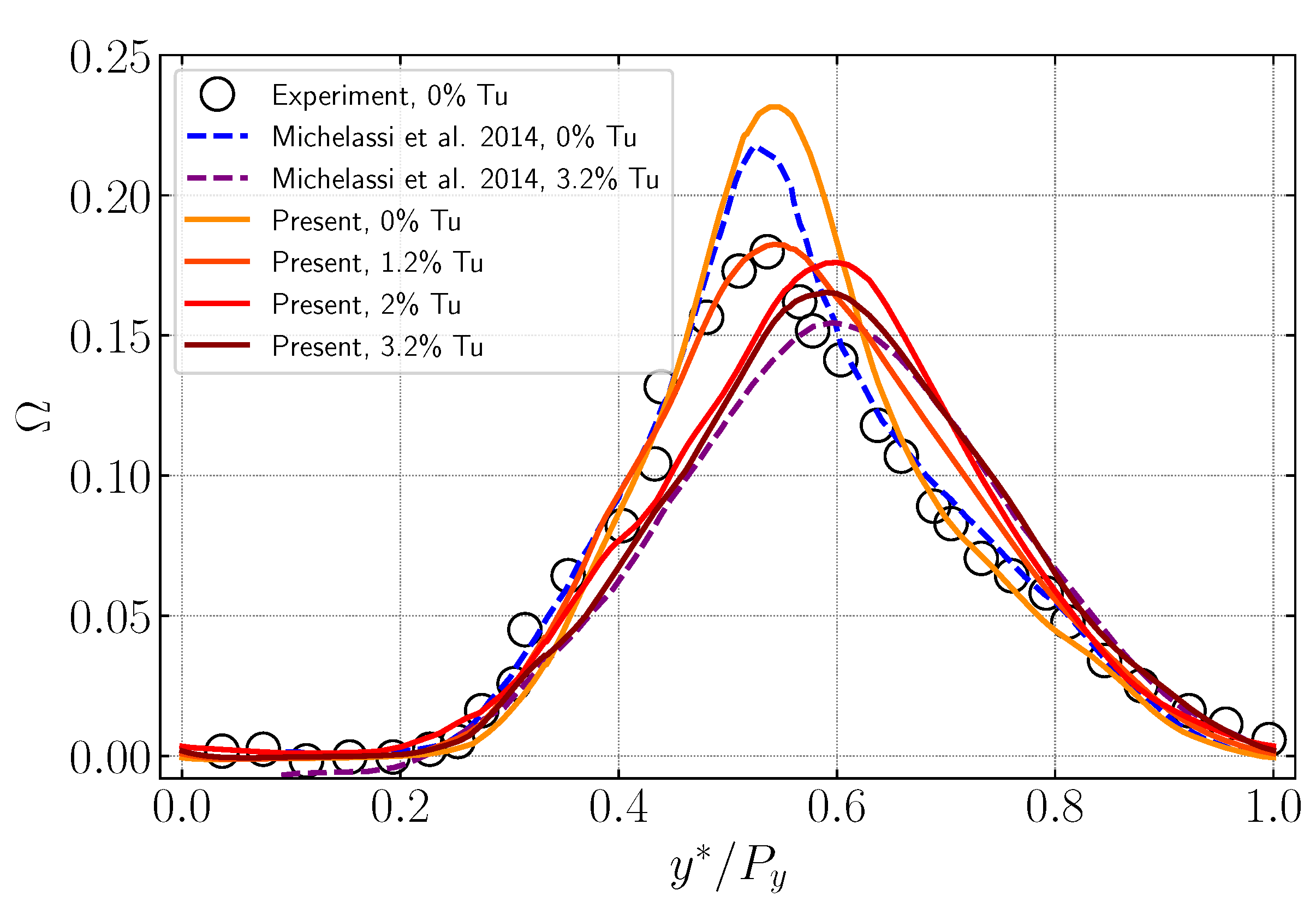
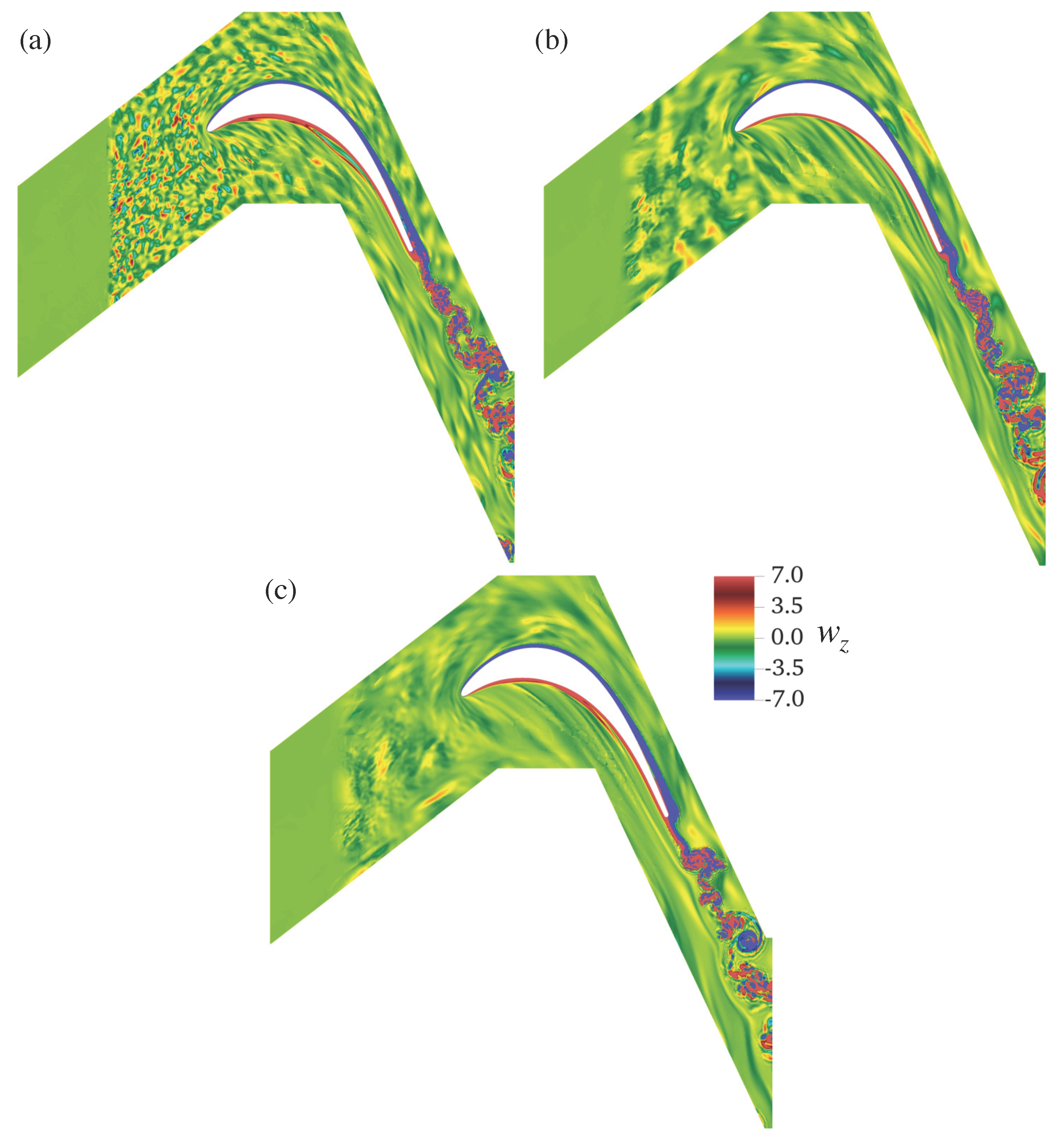
4.1. Dependence on Turbulence Intensity

A turbulence length scale of $5\%$ of the chord length was imposed in the synthetic turbulence generator for all simulations, meaning that no variation in the length scale was investigated here. Using this setup, 16 eddies were injected into the synthetic eddy region.

Figure 7 displays the turbulence intensity at the outlet plane of the synthetic eddy region along the pitchwise direction, showing the level of turbulence intensity at the moment the eddies were released from the synthetic eddy region. It can be seen that, for all turbulence intensity values employed in this study, the fluctuations oscillate around the imposed values set by the synthetic turbulence generator. The average turbulence intensities for $1.2\%$, $2\%$, and $3.2\%$ are $1.29\%$, $2.03\%$, and $3.23\%$, respectively. Note that turbulence intensity is a statistical quantity, meaning that a more precise and accurate result could have been obtained if the solution had been time-averaged over a longer period. This result further validates the implementation, demonstrating that the method accurately injects the correct turbulence intensity into the flow field.

Skin friction is depicted in Figure 8. For a clean flow field, the separation point occurs near the trailing edge at approximately $0.795C_{ax}$, which is just slightly downstream of the location predicted by Garai et al. [5], which demonstrates the accuracy of our model. Three key observations can be made here regarding the turbulence intensity. First, as turbulence intensity increases, the separation point shifts downstream towards the trailing edge. This occurs because higher turbulence intensity introduces stronger eddies into the flow field, which leads to a turbulent downstream flow, as expected. Since the turbulent flow is more energetic, it has more energy to energise the boundary layer, enhancing its stability and delaying separation, which allows the boundary layer to flow farther downstream before separating and transitioning into a turbulent boundary layer. Second, for turbulence intensities greater than $2\%$, there is no reattachment, leading to an open bubble forming on the blade surface near the trailing edge. Finally, the bubble shortens as the turbulence intensity increases, a phenomenon also reported by Michelassi et al. [3].

Figure 9 presents the pressure coefficient on the blade surface. Figure 9a compares the pressure coefficient with computational and experimental data from the literature. There is a notable level of agreement on the pressure distribution between experimental data [40] and DNS simulations [3]. It is interesting to notice that the levels of turbulence intensity imposed in the flow field were only able to slightly change the pressure distribution close to the trailing edge. A close-up of the pressure distribution around the trailing edge is shown in Figure 9b. Downstream of the separation point, the pressure curves increase slightly until they reach the region where the clean and $1.2\%$ turbulence intensity cases reattach. Note that for the cases that exhibit reattachment, the curves share approximately the same slope. However, the $2\%$ and $3.2\%$ turbulence intensity cases, which present open bubbles, display a steeper slope closer to the end of the trailing edge, with the case of the highest turbulence intensity exhibiting the steepest slope.

We now move on to the wake loss profiles in Figure 10, measured $0.4C$ downstream of the trailing edge. Note that, as discussed by Garai et al. [5], the numerical wake loss profiles were shifted to align with the peak position of the experimental wake loss, since the experiments do not document the exact pitch location of the peak loss. This mismatch in the wake loss profile is attributed to the low turbulence in the clean case of the experiments. Therefore, we use $y^{*}$ to denote the pitchwise position, as the numerical data were shifted. We can see that the clean inflow simulation over-predicts the maximum value of the wake loss compared to experimental data [40]. However, it shows very good agreement with other DNS simulations [2,3]. At $1.2\%$ Tu, the wake peak drops, reaching the same value as reported in Stadtmuller [40], which might be explained by the fact that, in experiments, there is always a low level of turbulence in the flow field [1,4,5]. It should also be noted that these results show great agreement regarding the suction side of the wake profile. As the turbulence intensity increases, it is easy to see that the wake loss profile approaches the results obtained by Michelassi et al. [3] for $3.2\%$ Tu, almost overlapping the curves.

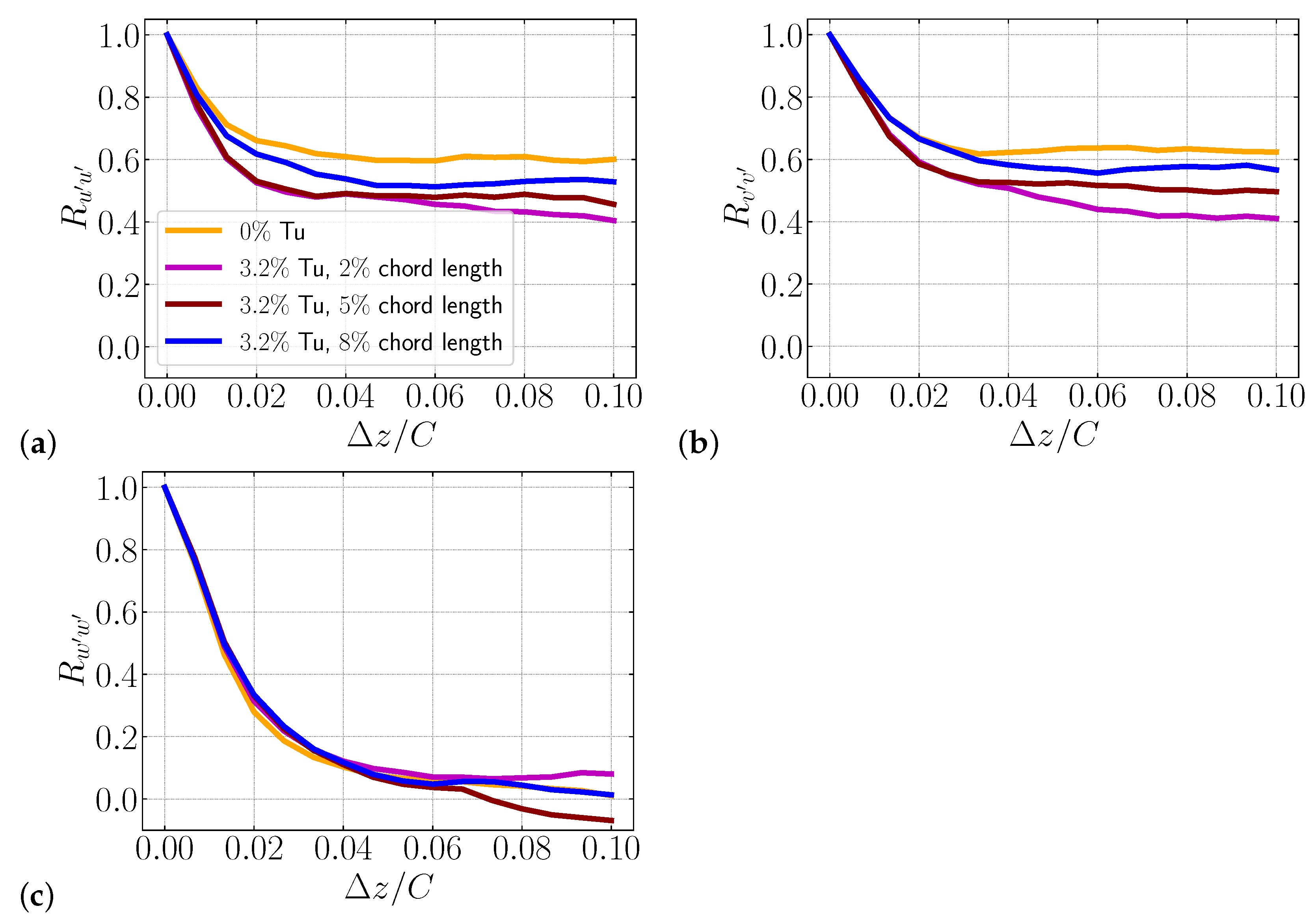
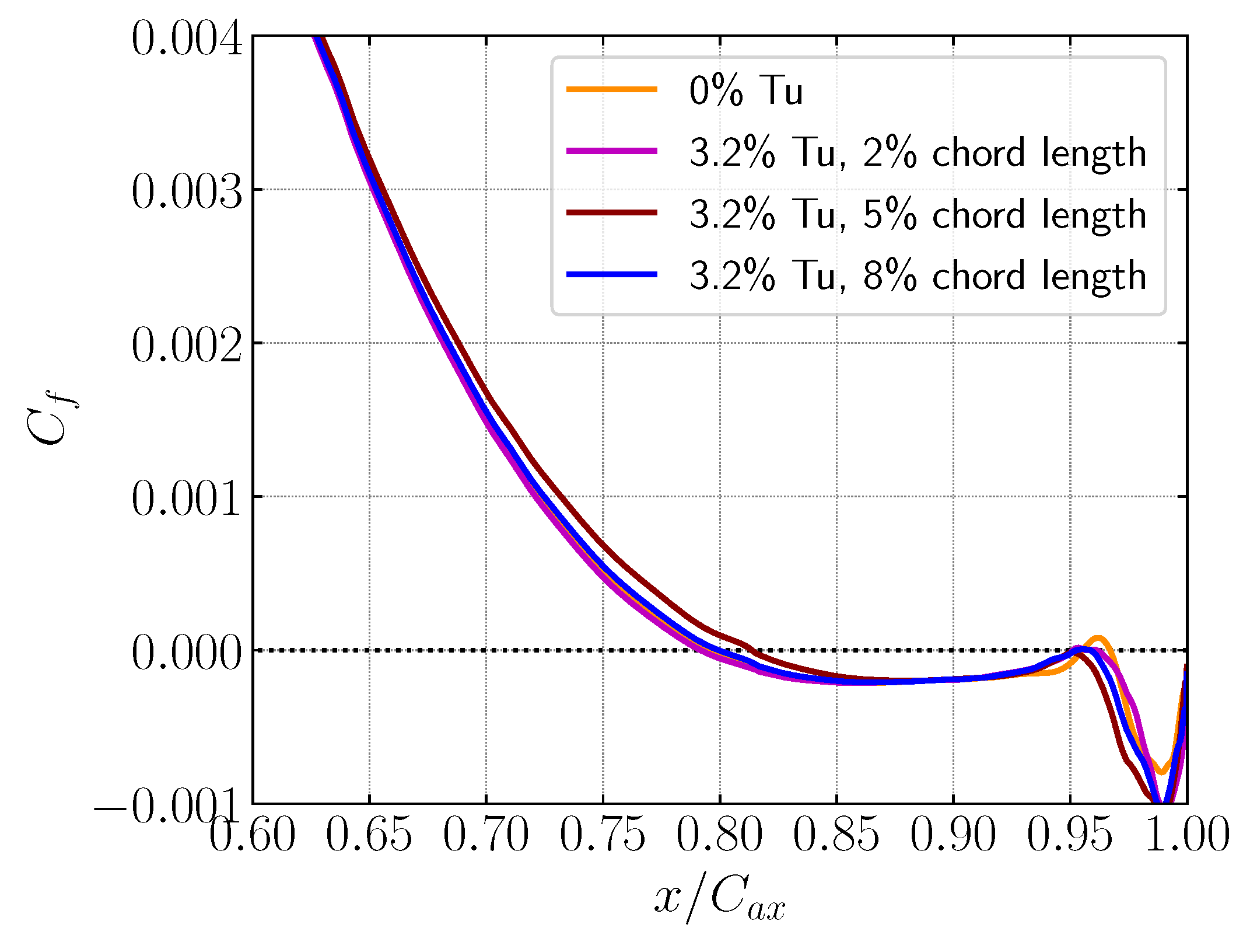
4.2. Dependence on Turbulence Length Scale

Now, we examine the effects of inflow turbulence with different turbulence length scales on the transition processes, wake behaviours, and pressure losses. Two additional turbulence length scales are considered. These new scales correspond to $2\%$ and $8\%$ of the chord length, resulting in the injection of 100 and 7 eddies, respectively, into the synthetic eddy regions. Note that, although the turbulence length scale was varied, the turbulence intensity was kept constant at $3.2\%$ in this section. Figure 11 illustrates the spanwise vorticity of the flow field for various turbulence length scales at $3.2\%$ Tu. It can be seen that, depending on the turbulence length scale generated in the flow field, it can trigger distinct wake behaviours. The wake for the $8\%$ chord length demonstrates less mixing compared to the other cases. Interestingly, this is the only length scale that produces a well-behaved vortex (negative vortex in blue) downstream of the trailing edge in Figure 11c. On the other hand, for the $2\%$ and $5\%$ chord lengths, the wakes appear to generate more mixing and exhibit greater turbulence.

In order to further understand the wake behaviour for different turbulence length scales, the spanwise two-point correlation at $x/C=0.074$ downstream of the trailing edge is displayed in Figure 12. Analysing the $8\%$ chord-length case in Figure 12a,b, it is clear that the correlations of the u and v components are the closest to the clean case, indicating that this turbulence length scale has little effect on the wake behaviour, particularly for the v component. These findings are in agreement with the previously discussed flow field shown in Figure 11c, which displays less mixing downstream of the trailing edge. In contrast, the $2\%$ and $5\%$ chord-length cases exhibit higher decorrelation compared to the clean case, which explains the stronger breakdown of the wake and increased turbulence downstream. Considering the w component, all of the curves demonstrate similar behaviour, although the $5\%$ chord-length case shows the highest decorrelation, at $\mathrm{\Delta }z/C=0.1$.

Figure 13 shows the skin friction on the surface for different turbulence length scales at $3.2\%$ Tu. Notably, at a turbulence length scale of $2\%$ of the chord length, the separation point occurs earlier than in the clean simulation ($0\%$ Tu). In addition, the separation bubble remains nearly the same size compared with the clean case. This demonstrates that this length scale does not energise the boundary layer, even though smaller scales may more easily penetrate the boundary layer. At $5\%$ chord length, the separation point occurs later than in the $2\%$ and $8\%$ cases. This suggests that, at this length scale, the turbulence was able to trigger the characteristic length scale of the boundary layer, resulting in the separation point occurring farther downstream due to a more energetic boundary layer. It should be noted that the $2\%$ and $8\%$ chord-length cases exhibit reattachment, whereas the $5\%$ chord-length case does not, as discussed in Figure 8. This indicates that the turbulence length scale is a dominant factor in predicting flow separation and reattachment. Also, no trend was observed in the skin friction when the turbulence length scale changed, which further highlights the fact that, at $5\%$ chord length, the boundary layer may have been energised. Furthermore, it is interesting to note that the skin friction at $5\%$ chord length starts to deviate from the other two curves at $x/C_{ax}=0.65$, although they have the same turbulence intensity.

Wall-normal profiles of the mean tangential velocity along with the boundary-layer height and turbulence intensity are shown in Figure 14. The separation point corresponds to the $5\%$ turbulence length-scale case, which occurs at $x/C_{ax}=0.814$. In Figure 14a, it can be seen that the mean tangential velocity profile remains practically unchanged for different length scales, even after separation, except for the $5\%$ chord-length case, which exhibited a slightly different profile after $x/C_{ax}=0.87$. Examining the boundary-layer height, it is evident that upstream of the separation, the boundary-layer height is approximately $4\%$ of the chord length. This explains why the $5\%$ chord-length case was able to better energise the boundary layer and delay both separation and transition compared to the other turbulence length scales (Figure 13). The $5\%$ chord length corresponds to the turbulence length scale closest to the boundary-layer length scale before separation, which contributes more significantly to this effect.

Looking at the turbulence intensity on the boundary layer in Figure 14b, it is easy to see that the clean case exhibits significantly lower turbulence intensity before and after separation compared to the cases with imposed turbulence. A notable observation in the turbulence intensity profile is that, as also reported by Garai et al. [5], higher turbulence intensity after separation occurs in the separated shear layer. In addition, it can be seen that the $2\%$ chord-length case demonstrates a lower turbulence intensity close to the boundary-layer surface (bubble), exhibiting behaviour similar to that in the clean case; however, the turbulence intensity is the highest in the separated shear layer at $x/C_{ax}=0.87$ and $x/C_{ax}=0.93$. The cases with $5\%$ and $8\%$ chord lengths show the highest levels of turbulence intensity close to the trailing edge and blade surface, exhibiting similar behaviour overall.

Figure 15 shows the instantaneous spanwise shear stress on the suction surface under different turbulence length scales. When the synthetic inflow turbulence injects eddies into the flow field, three-dimensionalities can be easily observed near the leading edge of the suction side of the blades, which do not appear in the clean case (Figure 15a). Moving through the blade surface, the three-dimensional dynamics persist until the flow separates. It is quite evident that the cases with $2\%$ and $5\%$ chord lengths have the highest rate of turbulence penetration into the boundary layer and intensity, since these length scales are smaller than or of the order of the boundary-layer height.

Instantaneous streamwise shear stresses on the suction surface at $3.2\%$ Tu for different turbulence length scales are shown in Figure 16. The blade surface is displayed from the leading edge to the separation point in the clean case ($x/C_{ax}=0.795$). In Figure 16a, as previously discussed for the $2\%$ chord-length case, smaller instabilities penetrate the boundary layer. This is captured by the streamwise shear stress as local maxima and minima on the blade surface within the acceleration region. It is important to note that, at this turbulence length scale, these small-scale perturbations dissipate quickly but re-energise small structures as they vanish. However, at the $8\%$ chord length, as seen in Figure 16c, smaller scales are excited within the boundary layer (indicated by the dashed ellipse), demonstrating the breakdown of larger perturbations into smaller scales of turbulence, despite the characteristic turbulence length scale being $8\%$ of the chord length. Also note that the larger length scales take longer to break down, then energise smaller structures. It is worth mentioning that all length scales were observed in the three cases examined here, with the dominant scale of each being driven by the turbulence generator.

The perturbations close to the end of the acceleration region (or separation point) highlighted by the continuous ellipses in each case reflect the fact that when the turbulence length scale is on the order of the characteristic length scale of the boundary-layer height before transition (Figure 14a), its effect on the boundary layer may be amplified, affecting the separation point, separation bubble, and transition. Note that these perturbation features (length scales) are driven by the turbulence generator, which feeds the flow field with the desired length scale. This discussion highlights the significant impact that the turbulence length scale can have on the flow dynamics over the blade surface, demonstrating that the turbulence intensity is not the sole factor influencing separation and transition in low-pressure turbine blades.

The wake losses for different turbulence length scales at $3.2\%$ Tu are shown in Figure 17. It can be observed that the turbulence length scale has a moderate effect on the wake loss. Although the pressure side of the wake loss exhibits behaviour across all three cases, the suction side shows different behaviours. The $2\%$ and $8\%$ chord-length cases follow equivalent trends, except at the peak value, where the $2\%$ chord-length case has a higher value. This reinforces the argument that, at the $2\%$ length scale, the smaller structures had little effect on the transition of the boundary layer, whereas at the 8% length scale, the structures may break down into smaller scales and energise the boundary layer. It should be noted that the case with $2\%$ Tu and $5\%$ turbulence length scales demonstrates a higher wake loss effect on the suction side than the case with $3.2\%$ Tu and $2\%$ turbulence length scales, as seen in Figure 10 and Figure 17. This illustrates a scenario where a lower turbulence intensity produces a greater influence on wake loss. Finally, we observe that the wake loss at $3.2\%$ Tu and $5\%$ of the chord length experiences the most significant effect, resulting in lower pressure losses compared to the other cases. Hence, it reveals that the turbulence length scale also has a dominant influence on the wake loss profile, not only the turbulence intensity.

5. Conclusions

Numerical simulations of the T106A low-pressure turbine in the DNS range were conducted for various turbulence intensities and length scales. The discontinuous Galerkin method was employed for the spatial discretisation of the compressible Navier–Stokes solver, and an implicit time-integration method was used to evolve the simulations over time. Additionally, a sponge layer was applied throughout the domain, covering the inflow and outflow regions to prevent acoustic reflections from the boundary conditions. To introduce anisotropic turbulence into the flow field, a source-term formulation of the SEM was implemented and validated within the Nektar++ framework.

The source-term formulation of the SEM implemented here has proven capable of reproducing the main results from the literature, demonstrating that this approach is reliable and precise for injecting turbulence in turbomachinery-related flow cases. It is worth mentioning that this methodology is not only efficient but can also reduce computational cost for computationally intensive simulation, since the inflow turbulence is not introduced in the inlet boundary condition, which avoids unnecessary mesh refinement in the inlet region. Complementing the low-pressure turbine model, a single sponge layer was implemented, covering the inflow and outflow regions. In other words, the sponge layer acts downstream of the inflow boundary and upstream of the outflow boundary to prevent acoustic wave reflections under boundary conditionssuch that it improves numerical stability. Additionally, leveraging the capability of Nektar++ to assign different polynomial orders to adjacent elements, a lower polynomial order was used just upstream of the outflow boundary to diffuse the vortices and turbulence from the wake by coarsening the mesh. In conclusion, the combination of these three strategies made our methodology robust and efficient.

Analysing the influence of turbulence intensity levels in the flow field, the results demonstrate that turbulence intensity plays a significant role in determining the flow characteristics and loss mechanisms in a low-pressure turbine. The increase in turbulence intensity leads to a delayed separation point and a reduced size of the separation bubble, influencing the wake loss profiles. These results are consistent with previous experimental and DNS results, confirming the accuracy of our methodology. Additionally, the peak wake loss value decreases, and the outflow angle changes as the turbulence intensity increases, aligning with experimental and DNS observations and highlighting the effect of turbulence intensity.

We can conclude from this study that the influence of the turbulence length scale on the overall flow behaviour of the turbine blade is as significant as that of turbulence intensity. The turbulence length scale plays a crucial role in flow separation, transition, wake mixing, and the wake loss profile. As observed in the spanwise vorticity flow fields and correlations, smaller length scales lead to higher levels of turbulence and mixing downstream of the trailing edge. This occurs because smaller scales, relative to the boundary-layer height, penetrate more easily into the boundary layer. However, the smallest turbulence length scales applied in this study did not have a significant influence on transition or the wake profile. In contrast, a turbulence length scale on the order of the boundary-layer height before transition was able to sufficiently energise the boundary layer, resulting in delayed flow separation and transition with an open bubble. Additionally, its wake profile was most affected by the synthetic turbulence generator.

References

1. Sandberg, R.; Pichler, R.; Chen, L. Assessing the sensitivity of turbine cascade flow to inflow disturbances using direct numerical simulation. In Proceedings of the 13th International Symposium for Unsteady Aerodynamics, Tokyo, Japan, 11–14 September 2012. [Google Scholar]
2. Sandberg, R.D.; Pichler, R.; Chen, L.; Johnstone, R.; Michelassi, V. Compressible direct numerical simulation of low-pressure turbines: Part I—Methodology. In Proceedings of the ASME Turbo Expo 2014, Düsseldorf, Germany, 16–20 June 2014; p. V02DT44A013. [Google Scholar] [CrossRef]
3. Michelassi, V.; Johnstone, R.; Pichler, R.; Chen, L.; Sandberg, R.D. Compressible direct numerical simulation of low-pressure turbines: Part II—Effect of inflow disturbances. In Proceedings of the ASME Turbo Expo 2014, Düsseldorf, Germany, 16–20 June 2014; p. V02DT44A014. [Google Scholar] [CrossRef]
4. Garai, A.; Diosady, L.T.; Murman, S.M.; Madavan, N.K. DNS of flow in a low-pressure turbine cascade using a discontinuous-Galerkin spectral-element method. In Proceedings of the ASME Turbo Expo 2015, Montréal, QC, Canada, 15–19 June 2015; p. V02BT39A023. [Google Scholar] [CrossRef]
5. Garai, A.; Diosady, L.T.; Murman, S.M.; Madavan, N.K. DNS of low-pressure turbine cascade flows with elevated inflow turbulence using a discontinuous-Galerkin spectral-element method. In Proceedings of the ASME Turbo Expo 2016, Seoul, Republic of Korea, 13–17 June 2016; p. V02CT39A025. [Google Scholar] [CrossRef]
6. Michelassi, V.; Chen, L.; Pichler, R.; Sandberg, R.D.; Bhaskara, R. High-fidelity simulations of low-pressure turbines: Effect of flow coefficient and reduced frequency on losses. J. Turbomach. 2016, 138, 111006. [Google Scholar] [CrossRef]
7. Sandberg, R.D.; Michelassi, V. The current state of high-fidelity simulations for main gas path turbomachinery components and their industrial impact. Flow Turbul. Combust. 2019, 102, 797–848. [Google Scholar] [CrossRef]
8. Nakhchi, M.E.; Naung, S.W.; Rahmati, M. Direct numerical simulations of turbulent flow over low-pressure turbine blades with aeroelastic vibrations and inflow wakes. Energies 2023, 16, 2803. [Google Scholar] [CrossRef]
9. Bergmann, M.; Morsbach, C.; Klose, B.F.; Ashcroft, G.; Kugeler, E. A numerical test rig for turbomachinery flows based on large eddy simulations with a high-order discontinuous Galerkin scheme—Part I: Sliding interfaces and unsteady row interactions. J. Turbomach. 2023, 146, 021005. [Google Scholar] [CrossRef]
10. Morsbach, C.; Bergmann, M.; Tosun, A.; Klose, B.F.; Bechlars, P.; Kugeler, E. A numerical test rig for turbomachinery flows based on large eddy simulations with a high-order discontinuous Galerkin scheme—Part III: Secondary flow effects. J. Turbomach. 2023, 146, 021007. [Google Scholar] [CrossRef]
11. Isler, J.; Vivarelli, G.; Cantwell, C.; Montomoli, F.; Sherwin, S.; Frey, Y.; Meyer, M.; Vazquez, R. Source-term based synthetic turbulence generator applied to compressible DNS of the T106A low-pressure turbine. In Proceedings of the 16th European Conference on Turbomachinery Fluid Dynamics & Thermodynamics, Hannover, Germany, 24–28 March 2025. [Google Scholar]
12. Wheeler, A.P.S.; Sandberg, R.D.; Sandham, N.D.; Pichler, R.; Michelassi, V.; Laskowski, G. Direct numerical simulations of a high-pressure turbine vane. J. Turbomach. 2016, 138, 071003. [Google Scholar] [CrossRef]
13. Klose, B.F.; Morsbach, C.; Bergmann, M.; Hergt, A.; Klinner, J.; Grund, S.; Kugeler, E. A numerical test rig for turbomachinery flows based on large eddy simulations with a high-order discontinuous Galerkin scheme—Part II: Shock capturing and transonic flows. J. Turbomach. 2023, 146, 021006. [Google Scholar] [CrossRef]
14. Vivarelli, G.; Isler, J.A.; Williams, T.S.; Montomoli, F.; Sherwin, S.; Adami, P.; Vazquez, R. On the effect of curvature and compressibility in boundary layers over fan blades and engine intakes. In Proceedings of the 15th European Conference on Turbomachinery Fluid Dynamics & Thermodynamics, Budapest, Hungary, 24–28 April 2023. [Google Scholar] [CrossRef]
15. Isler, J.; Vivarelli, G.; Montomoli, F.; Sherwin, S.; Adami, P.; Vazquez, R. High fidelity compressible and incompressible flow simulations of a turbomachinery geometrical configuration. In Proceedings of the 15th European Conference on Turbomachinery Fluid Dynamics & Thermodynamics, Budapest, Hungary, 24–28 April 2023. [Google Scholar] [CrossRef]
16. Klein, M.; Sadiki, A.; Janicka, J. A digital filter based generation of inflow data for spatially developing direct numerical or large eddy simulations. J. Comput. Phys. 2003, 186, 652–665. [Google Scholar] [CrossRef]
17. Davidson, L. Using isotropic synthetic fluctuations as inlet boundary conditions for unsteady simulations. Adv. Appl. Fluid Mech. 2007, 1, 1–35. [Google Scholar]
18. Cassinelli, A.; Xu, H.; Montomoli, F.; Adami, P.; Diaz, R.V.; Sherwin, S.J. On the effect of inflow disturbances on the flow past a linear LPT vane using spectral/hp element methods. In Proceedings of the ASME Turbo Expo 2019, Phoenix, AZ, USA, 17–21 June 2019; p. V02CT41A032. [Google Scholar] [CrossRef]
19. Vivarelli, G.; Isler, J.A.; Montomoli, F.; Cantwell, C.; Sherwin, J.S.; Frey-Marioni, Y.; Vazquez-Diaz, R. Applications and recent developments of the open-source computational fluid dynamics high-fidelity spectral/hp element framework Nektar++ for turbomachinery configurations. In Proceedings of the ASME Turbo Expo 2024, London, UK, 24–28 June 2024; Volume 88070, p. V12CT32A022. [Google Scholar] [CrossRef]
20. Schmidt, S.; Breuer, M. Source term based synthetic turbulence inflow generator for eddy-resolving predictions of an airfoil flow including a laminar separation bubble. Comput. Fluids 2017, 146, 1–22. [Google Scholar] [CrossRef]
21. Giangaspero, G.; Withered, F.; Vincent, P. Synthetic turbulence generation for high-order scale-resolving simulations on unstructured grids. AIAA J. 2022, 60, 1032–1051. [Google Scholar] [CrossRef]
22. Yan, Z.G.; Pan, Y.; Castiglioni, G.; Hillewaert, K.; Peiró, J.; Moxey, D.; Sherwin, S. Nektar++: Design and implementation of an implicit, spectral/hp element, compressible flow solver using Jacobian-free Newton Krylov approach. Comput. Math. Appl. 2021, 81, 351–372. [Google Scholar] [CrossRef]
23. Cantwell, C.D.; Moxey, D.; Comerford, A.; Bolis, A.; Rocco, G.; Mengaldo, G.; De Grazia, D.; Yakovlev, S.; Lombard, J.E.; Ekelschot, D.; et al. Nektar++: An open-source spectral/hp element framework. Comput. Phys. Commun. 2015, 192, 205–219. [Google Scholar] [CrossRef]
24. Moxey, D.; Cantwell, C.D.; Bao, Y.; Cassinelli, A.; Castiglioni, G.; Chun, S.; Juda, E.; Kazemi, E.; Lackhove, K.; Marcon, J.; et al. Nektar++: Enhancing the capability and application of high-fidelity spectral/hp element methods. Comput. Phys. Commun. 2020, 249, 107110. [Google Scholar] [CrossRef]
25. Lindblad, D.; Isler, J.; Ginard, M.M.; Sherwin, S.J.; Cantwell, C.D. Nektar++: Development of the compressible flow solver for jet aeroacoustics. Comput. Phys. Commun. 2024, 300, 109203. [Google Scholar] [CrossRef]
26. Jarrin, N.; Benhamadouche, S.; Laurence, D.; Prosser, R. A synthetic-eddy-method for generating inflow conditions for large-eddy simulations. Int. J. Heat Fluid Flow 2006, 27, 585–593. [Google Scholar] [CrossRef]
27. Jarrin, N.; Prosser, R.; Uribe, T.C.; Benhamadouche, S.; Laurence, D. Reconstruction of turbulent fluctuations for hybrid RANS/LES simulations using a synthetic-eddy method. Int. J. Heat Fluid Flow 2009, 30, 435–442. [Google Scholar] [CrossRef]
28. Pamiès, M.; Weiss, P.E.; Garnier, E.; Deck, S.; Sagaut, P. Generation of synthetic turbulent inflow data for large eddy simulation of spatially evolving wall-bounded flows. Phys. Fluids 2009, 21, 045103. [Google Scholar] [CrossRef]
29. Giangaspero, G.; Amerio, L.; Downie, S.; Zasso, A.; Vincent, P. High-order scale-resolving simulations of extreme wind loads on a model high-rise building. J. Wind Eng. Ind. Aerodyn. 2022, 230, 105169. [Google Scholar] [CrossRef]
30. Shen, W.; Wang, Y.; Cui, J. Analysis of the effect of turbulent inflow on the flow-field and noise of supersonic jet flow using large eddy simulation. J. Sound Vib. 2024, 572, 118156. [Google Scholar] [CrossRef]
31. Caros, L.; Buxton, O.; Vincent, P. The effects of free-stream eddies on optimized Martian rotorcraft airfoils. In Proceedings of the AIAA SCITECH 2024 Forum, Orlando, FL, USA, 8–12 January 2024. [Google Scholar] [CrossRef]
32. Lund, T.S.; Wu, X.; Squires, K.D. Generation of turbulent inflow data for spatially-developing boundary layer simulations. J. Comput. Phys. 1998, 140, 233–258. [Google Scholar] [CrossRef]
33. Morkovin, M.V. Effects of compressibility on turbulent flows. Mécanique de la Turbulence 1962, 367, 380. [Google Scholar]
34. Kim, J.; Moin, P.; Moser, R. Turbulence statistics in fully developed channel flow at low Reynolds number. J. Fluid Mech. 1987, 177, 133–166. [Google Scholar] [CrossRef]
35. Moser, R.; Kim, J.; Mansour, N. Direct numerical simulation of turbulent channel flow up to Reτ=590. Phys. Fluids 1999, 11, 943–945. [Google Scholar] [CrossRef]
36. Georgiadis, N.J.; Rizzetta, D.P.; Fureby, C. Large-eddy simulation: Current capabilities, recommended practices, and future research. AIAA J. 2010, 48, 1772–1784. [Google Scholar] [CrossRef]
37. Kim, Y.; Castro, I.P.; Xie, Z.T. Divergence-free turbulence inflow conditions for large-eddy simulations with incompressible flow solvers. Comput. Fluids 2013, 84, 56–68. [Google Scholar] [CrossRef]
38. Patruno, L.; Miranda, S.D. Unsteady inflow conditions: A variationally based solution to the insurgence of pressure fluctuations. Comput. Methods Appl. Mech. Eng. 2020, 363, 112894. [Google Scholar] [CrossRef]
39. Robinson, S. Coherent motions in the turbulent boundary layer. Annu. Rev. Fluid Mech. 1991, 23, 601–639. [Google Scholar] [CrossRef]
40. Stadtmuller, P. Investigation of wake-induced transition on the LP turbine cascade T106A-EIZ. In DFG-Verbundprojekt Fo 136//11; University of the Armed Forces: Munich, Germany, 2001; Version 1.0. [Google Scholar]
41. Lyu, G.; Chen, C.; Du, X.; Sherwin, S.J. Stable, entropy-pressure compatible subsonic Riemann boundary condition for embedded DG compressible flow simulations. J. Comput. Phys. 2023, 476, 111896. [Google Scholar] [CrossRef]
42. Uranga, A.; Persson, P.O.; Drela, M.; Peraire, J. Implicit large eddy simulation of transition to turbulence at low Reynolds numbers using a discontinuous Galerkin method. Int. J. Numer. Methods Eng. 2011, 87, 232–261. [Google Scholar] [CrossRef]
Figure 1. Schematic setup of the plane channel flow and synthetic eddy region (not to scale).
Ijtpp 10 00013 g001
Figure 2. Displacement of an eddy (n) in the synthetic eddy region.
Ijtpp 10 00013 g002
Figure 3. Time and spanwise average profiles of (a) turbulent boundary-layer velocity ( U + = U / u τ ), (b) u r m s + = u r m s / u τ = u u 1 / 2 / u τ , (c) v r m s + = v r m s / u τ , (d) w r m s + = w r m s / u τ , (e) the Reynolds stress component acting on the face normal to the x axis in the y-direction, and (f) pressure variation correlation.
Ijtpp 10 00013 g003
Figure 4. Isosurface of Q criterion at Q = 0.75 U 2 / δ 2 , coloured by velocity magnitude. Flow is from the right to left. Only the lower half of the channel and part of the domain in the streamwise direction are shown.
Ijtpp 10 00013 g004
Figure 5. (a) Linear mesh and model of the T106A low-pressure turbine linear cascade. (b) Variable polynomial order around the outflow region. Polynomial order transition region from P = 3 to P = 2 .
Ijtpp 10 00013 g005
Figure 6. Near-wall mesh resolution along the suction and pressure surfaces for the T106A blade.
Ijtpp 10 00013 g006
Figure 7. Turbulence intensity at the outlet plane of the synthetic eddy region along the pitchwise direction.
Ijtpp 10 00013 g007
Figure 8. Skin friction on the blade surface for different turbulence intensities.
Ijtpp 10 00013 g008
Figure 9. (a) Pressure distribution on the blade surface. (b) Close-up of the trailing edge. Comparison with data from Michelassi et al. [3].
Ijtpp 10 00013 g009
Figure 10. Wake loss profiles 0.4 C downstream of the trailing edge. Comparison with data from Michelassi et al. [3].
Ijtpp 10 00013 g010
Figure 11. Instantaneous spanwise vorticity for 3.2 % Tu with turbulence length scales of (a) 2 % , (b) 5 % , and (c) 8 % of the chord length. The slices were taken from the three-dimensional flow fields at z / C = 0.16 .
Ijtpp 10 00013 g011
Figure 12. Spanwise two-point correlation at x / C = 0.074 downstream of the trailing edge for velocity components (a) u, (b) v, and (c) w with anisotropic turbulence length scales.
Ijtpp 10 00013 g012
Figure 13. Skin friction on the blade surface for the clean case and different turbulence length scales at 3.2% Tu.
Ijtpp 10 00013 g013
Figure 14. Wall-normal profiles of (a) mean tangential velocity, together with the boundary-layer height and (b) turbulence intensity (Tu), for the clean case and different turbulence length-scale cases at 3.2% Tu.
Ijtpp 10 00013 g014
Figure 15. Instantaneous spanwise shear stress on the suction surface for (a) the clean case and for 3.2 % Tu with turbulence length scales of (b) 2 % , (c) 5 % , and (d) 8 % of the chord length.
Ijtpp 10 00013 g015
Figure 16. Instantaneous streamwise shear stress on the suction surface for 3.2 % Tu with turbulence length scales of (a) 2 % , (b) 5 % , and (c) 8 % of the chord length. The blade is shown from the leading edge to the separation point for the clean case.
Ijtpp 10 00013 g016
Figure 17. Wake loss profiles for different turbulence length scales for 3.2% Tu.
Ijtpp 10 00013 g017
Disclaimer/Publisher’s Note: The statements, opinions and data contained in all publications are solely those of the individual author(s) and contributor(s) and not of MDPI and/or the editor(s). MDPI and/or the editor(s) disclaim responsibility for any injury to people or property resulting from any ideas, methods, instructions or products referred to in the content.