Application of Traffic Weighted Multi-Maps Based on Disjoint Routing Areas for Static Traffic Assignment

Abstract

Urban traffic congestion is a pressing issue, demanding effective and cost-efficient solutions. This paper develops the Traffic Weighted Multi-Maps (TWM) method to solve the Traffic Assignment Problem in Intelligent Transportation Systems (ITS). TWM offers drivers diverse views of the network, promoting path diversity and adaptability. Providing an optimal TWM configuration to the traffic demand in terms of structure and allocation policy is a challenging issue as it usually depends on the size of the network and its complexity. The paper explores TWM generation and assignment by applying routing areas based on semi-disjointed k-shortest paths and allocating them using a per-sub flow optimized assignment policy. This approach allows obtaining a pseudo-optimal solution for static traffic assignment with similar results in terms of total travel time compared to the direct solution of calculating optimal map weights and the theoretical system optimum. It offers a cost-effective solution valid for wide urban areas, as the TWM calculation depends on the variety of the traffic flows and the number of semi-disjoint routing areas considered instead of the network complexity and size. Urban network experiments with synthetic traffic demands are studied under different TWM adoption rates, comparing results with existing traffic assignment policies and estimation methods. It highlights its potential for enhancing urban traffic management. Overall, TWM presents a promising approach to addressing urban traffic congestion efficiently.

1. Introduction

Traffic congestion avoidance is a crucial concern of modern urban mobility systems. A substantial effort is made to find effective solutions for congestion mitigation at reasonable costs. Congestion not only implies a considerable waste of productive time but also an enormous waste of energy and fuel and is the cause of a considerable volume of gas emissions. The USA Environmental Protection Agency (EPA) [1] states that “Greenhouse gas (GHG) emissions from transportation account for about 27 percent of total U.S. greenhouse gas emissions, making it the largest contributor to U.S. GHG emissions. Between 1990 and 2020, GHG emissions in the transportation sector increased more in absolute terms than in any other sector”. The European Union’s Clean Transport, Urban Transport Directive [2] identifies that urban congestion has a cumulative annual cost of 100 trillion EUR. Sixty percent of the European population lives in urban areas with more than 10,000 inhabitants. Likewise, urban mobility is estimated to be responsible for 40% of CO${}_2$ emissions and up to 70% of other pollutants. Government and state agencies play a critical role in traffic management, planning, ordering, and operation [3].

Intelligent Transportation Systems (ITS) are commonly used for urban traffic planning and operation, where the design and delivery of optimal routes to drivers is one of the key issues to solve and is known as the Traffic Assignment Problem (TAP) [4]. It is a well-characterized, mathematically complex, non-derivable, and convex problem, as the decision of each driver at each moment modifies the working conditions of the network. It forces the rest of the drivers to react to the changes and adapt their routing decisions. The system evolves until an equilibrium condition is met. For this reason, the resolution of the TAP has usually been approximated by heuristic methods, such as traffic assignment methods.

Traffic assignment methods abstract TAP as a supply and demand problem as pointed out in [5]. Vehicle trips (demand) are assigned to the traffic network (supply) by strategically performing route choices. There are multiple traffic assignment methods to model trip mapping into the network, either static or dynamic (DTA), and using direct or stochastic estimations [6]. They usually consume expensive computation resources as optimal paths must be calculated multiple times in an iterative way as the traffic network becomes loaded. Szeto and Wong [7] compiled an extensive comparative study of the equilibrium and assignment methods. Traffic assignment methods provide a theoretical framework for studying practical ITS implementations or simulations to see their effectiveness when comparing their behavior with equilibrium situations.

Classical traffic assignment and routing works consider that all the drivers share the same network view (map), assuming this is a fundamental hypothesis. Thus, algorithms rely on it and focus on other topics, such as edge occupancy and toll costs. The Traffic Weighted Multi-Maps (TWM) strategy was presented in [8] as an innovative mechanism of generating and distributing a set of complementary views of the traffic network to the drivers to generate path diversity chosen directly by the drivers. Moreover, TWM can be generated ad hoc for special traffic network conditions such as accidents or road cuts. TWM differs from other routing and traffic planning and assignment methods, providing network views as maps implementing user utility functions, system optimum constraints, dynamic reactions events, or any other type of information. TWM could also be interpreted as upgrading standard traffic signaling methods (fixed or dynamic panels), including a broader range of use cases. It is compatible with any other practical ITS implementations and can be directly integrated with them as it focuses on the map layers they all use.

Finding the right TWM configuration is a key challenge, and the first approaches were focused on how to obtain optimal TWM link weights (costs) based on driving needs, regulations, network constraints, and congestion conditions. Optimization techniques have been explored, such as genetic (GA) or particle swarm algorithms [9,10]. They provide good results for small or mid-size traffic networks. However, finding an optimal TWM for a graph containing E edge weights for a set of M maps is an $O(E\ast M)$ complexity resolution problem. GA applied to TWM becomes computationally unaffordable for more extensive networks (see Loder et al. [11] for city references).

Beyond the optimal TWM generation studies, this paper explores a different heuristic approach for the TAP using TWM. The initial hypothesis considers that the main traffic flows in the network can be predicted based on historical data, so it could be possible to generate also predefined TWM based on the k-Shortest Paths for these flows and obtain the optimal TWM assignment for the vehicles toward a system optimum. Each driver can make the best routing decision considering the map view received and the road occupation status. TWM generation based on k-Shortest Paths (TWM(kSP)) and optimal path-flow distribution was presented as a preliminary concept in [12].

In most real networks, the k-Shortest Paths (kSP) between two nodes have subtle differences of one or two edges with minimal impact on the cost of the final path. As edges become congested, vehicles will select the following lowest-cost links. However, most of the links will remain in common. In some way, this route selection strategy induces congestion, as it does not promote route variety [13,14]. Using K-Shortest Paths with a certain level of overlapping (Semi-Disjoint Shortest Paths, hereafter, Dj-kSP) allows the use of routing alternatives more decoupled from the progressive congestion of the paths.

This paper’s initial hypothesis is expanded to cover the TWM generation based on Semi-Disjoint Shortest Paths and the optimal TWM assignment depending on the drivers’ adherence to the routing method. Using Dj-kSP-based TWM should generate a greater route variety for the drivers, resulting in lower total travel time. Results should improve the direct k-Shortest Path and the TWM(k-SP) route assignment and approach the theoretical system optimum estimation. Additionally, optimal TWM assignment should enhance the performance of the optimal TWM generation strategy [15] as the complexity of the problem is considerably reduced.

Considering that an M map set has been designed to route the different F traffic flows for V vehicles that use the traffic network, it is necessary to find the optimal map assignment for the drivers, a problem of $O(V\ast M)$ complexity. This complexity may be reduced to $O(F\ast M)$ when considering traffic flows instead of individuals. The TWM maps used for flow routing can be efficiently achieved using pseudo-optimal routes based on semi-disjoint shortest paths (paths with limited overlap) obtained by the ESX-C algorithm described in [16,17].

Figure 1 provides a schematic overview of the Dj-kSP-based TWM map generation and distribution for traffic assignment. In this sense, this paper addresses:

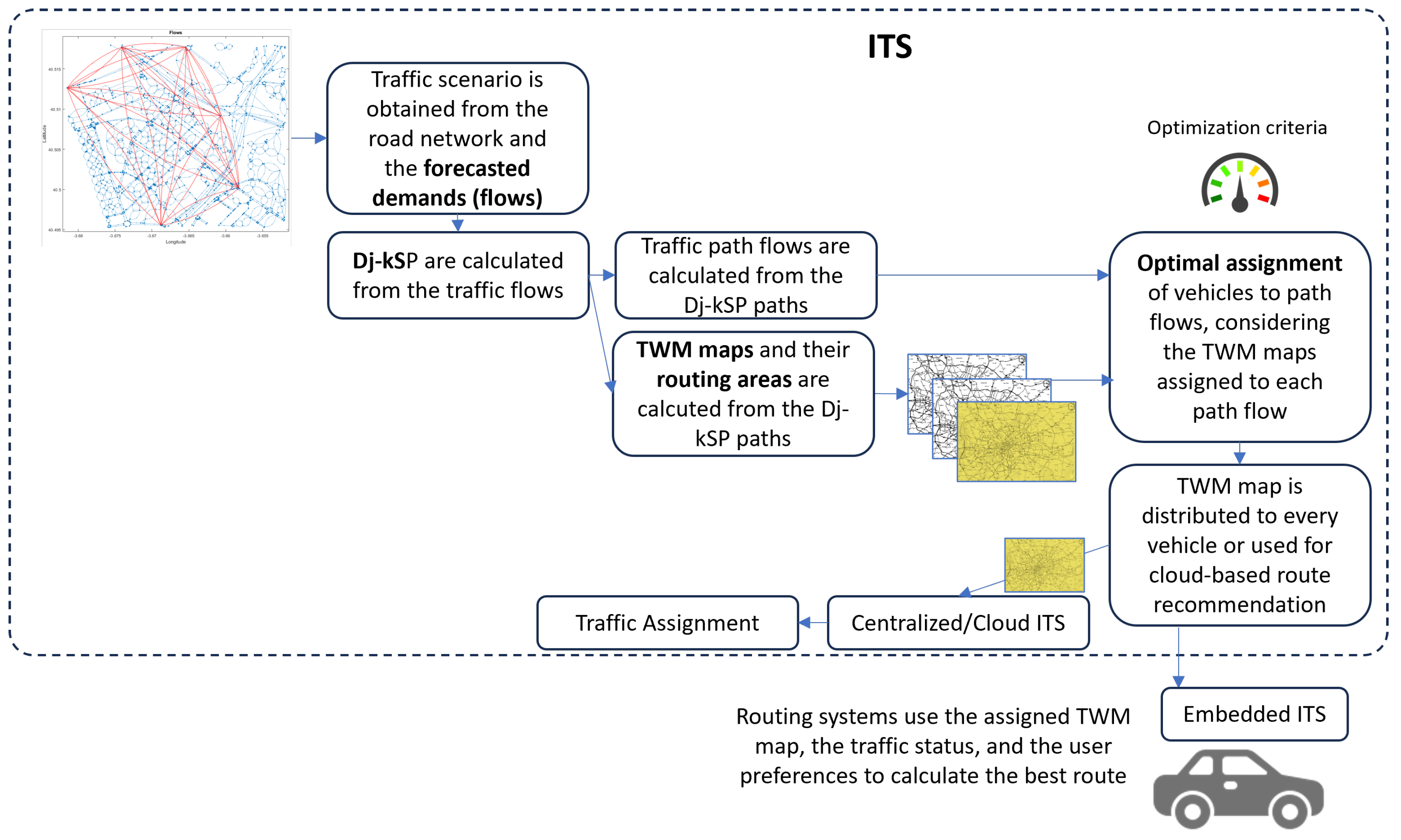
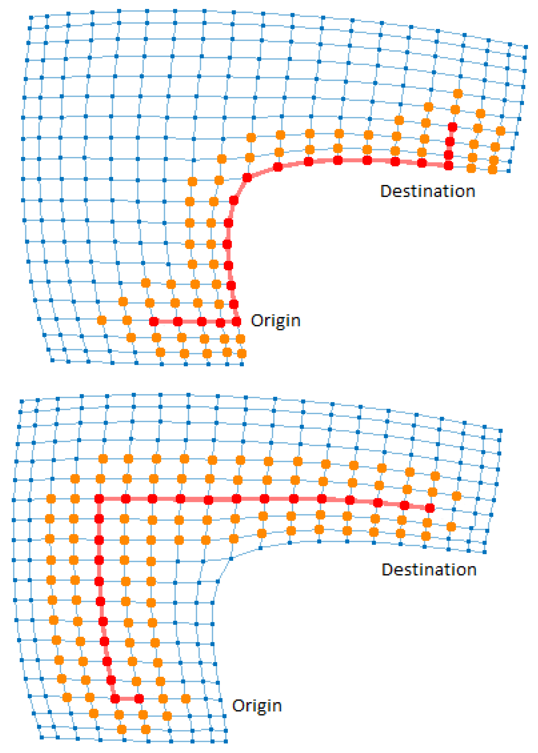
• A new method to create TWM map sets based on traffic flows, using the semi-disjoint k-shortest paths (Dj-kSP) linking their origin/destination nodes [13,18]. These semi-disjoint k-shortest paths define the best low-overlapping routes for each flow and are used to create routing zones that promote traffic usage through them.
• A study for optimal TWM assignment to the vehicles using a per-flow strategy. Optimization is achieved by applying genetic evolutionary algorithms (GA), to find which flow amounts will receive each TWM map.
• An empirical study for real urban networks with synthetic traffic demands, comparing the results with basic traffic assignment policies for lower and higher bounds such as free-flow and all-or-nothing routing methods [5], and with system optimum estimation methods such as Successive Averages Method (MSA), Cumulative Assignment Method (CAM) [5] or the linear programming method proposed by Wei [19].
• A discussion about the obtained results and the computing complexity of the different approaches. Calculating TWM maps based on routing areas around Dj-kSP seems to be a cost-effective solution for the problem. An initial optimal TWM distribution based on the Dj-kSP routes provides a good enough solution like a full TWM distribution optimization, thus offering a practical heuristic solution to the problem.

Transit traffic is a main urban traffic demand component [4,20], refers to the movement of people within the metropolitan areas, using public multi-modal transport such as buses, trams, light rail, subways, and commuter trains. Urban traffic planning needs to address the challenges of congestion, environmental concerns, and the efficient movement of many people, dealing with route design, schedule and frequency of service, fare structures, integration with other modes of transportation, accessibility, safety, and user experience [21,22]. TWM may be efficiently used for transit management with specific policies. Though it is out of the scope of this work, it constitutes a challenge for future research.

The next Section 2 reviews the state-of-the-art and previous works. Section 3 describes the TWM and path flow model, and the optimization strategies are discussed in Section 4. Section 5 describes the materials and methods used in the research. Section 6 describes the experimental use cases and results, and finally, Section 8 points out conclusions and future research directions.

2. Related Work

Traffic assignment deals with the distribution of a given traffic demand in a network following ideal driver’s behaviors. Static traffic assignment is based on Wardrop’s user equilibrium (UE) and system optimum (SO) principles [23]. There is a huge amount of literature on traffic assignment concepts and methods [5,6,24,25].

User equilibrium entails a user-centric traffic assignment, where each individual selfishly selects the most convenient route. This principle ensures fairness among users, as all individuals sharing a common origin and destination encounter identical travel times upon reaching equilibrium. However, a significant drawback of user equilibrium is that it fails to minimize the overall system travel time, leading to the incurrence of the “Price of Anarchy” (PoA) [26].

Sheffi [20] furnishes evidence establishing the user equilibrium’s existence and uniqueness. Lujak et al. [27] extend this by proving that this equilibrium aligns with a Nash equilibrium within a game involving many players. The stochastic version of the user equilibrium introduced in [20] considers drivers with incomplete information and less than complete rationality. Mirchandani and Soroush [28] proposed a model based on the expected utility theory. In the same direction, the travel time budget model was proposed by [29], the late arrival penalty model presented in [30], and the prospect-based user equilibrium model introduced at [31]. The ambiguity of driver travel time perception was handled using fuzzy decision techniques [32,33,34].

In contrast, the system optimum represents an efficient network-wide traffic assignment. Here, drivers are directed through the network in a manner that minimizes the total travel time. Nonetheless, users might encounter travel durations surpassing those of fellow travelers journeying from the same origin and destination, impacting overall compliance. Consequently, the limitations of either of these two approaches can be surmounted by amalgamating them, striving to establish a connection between user fairness and system-wide efficiency.

The calculation of the optimal solution involves solving the TAP. It is an NP-hard problem, so heuristic approximate methods are used, such as the cumulative assignment method (CAM), the successive averages method (MSA), or the Frank-Wolfe algorithm [5]. Second-order cone and linear programming (LP) approaches have recently been proposed [19] with a very efficient calculation. Constrained SO (CSO) was presented by Jahn [35], where length-bounded alternatives were offered to the drivers. The impact of choosing a CSO traffic assignment is described in [36], where a theoretical work on efficiency and fairness is proposed.

Jalota et al. [37] recently created an efficient method based on interpolation between SO and UE considering the Constrained System Optimum (CSO) defined by Jahn [35] and bounding the route unfairness.

Dynamic traffic assignment (DTA) deals with the time-varying traffic conditions, leading to dynamic user equilibrium (DUE). Additional stochastic models are used to model the user’s perception and travel time uncertainty, leading to stochastic user equilibrium (SUE) [7].

Route diversification is a critical factor in reducing congestion in traffic assignment. Kafani and Al-Deek [38] demonstrated the effects of an intelligent vehicle routing strategy on the performance and utilization of the traffic network in relation to system optimum in terms of overall transit times and congestion. Guidance diverts traffic from the freeway using a freeway overlaid on city streets when its marginal cost exceeds streets. Managing street speeds was a key finding for this routing guidance, though practical general implementation was not suggested.

Modifying edge costs through the design of tolls has also been one of the mechanisms employed for diversifying routes and leading to system optimality [39,40]. Ref. [41] considers the origin and destination tuples for the tolling service. In all cases, a microscopic simulation is used.

Synthetic route cost modification by the ITS needs to be balanced with the driver’s experience who takes the routing decision considering factors such as available network status information, previous experiences, or subjective concerns, as pointed out in [34,42].

Traffic Weighted Multi-maps (TWM) consider that drivers with different usage needs and concerns (utility functions), may receive different network maps. It takes into account that a map is just a view of the (urban) traffic network composed of (a) a physical layer for the topology of paths, junctions, and crossings, (b) a logical layer with management conventions and rules (sense, speed, constraints, prohibitions, and others.), and (c) a status/usage layer [34] showing network occupancy. An ITS generates a TWM comprising a set of map views for the same area (same physical layer) and a modified logical view formed by a distribution of edge/link weights based on the original network map ones. The so-formed multi-map (TWM) is distributed to traffic groups to create differentiated routing. Other related experiences have also pointed to map transformation procedures to generate alternative routes [43].

This technique may be applied to multiple use cases such as multi-objective travel optimization, congestion reduction, incident management, per fleet differential routing, and others [8]. Beyond these use cases, congestion management is a fundamental concern to transportation mobility linked to traffic equilibrium situations. TWM is a feasible technique compatible with both approaches as it combines different perspectives: (a) traffic network topology; (b) trip data (past and predictions); (c) usage costs; and (d) vehicle/trip segmentation based on activity models.

TWM can be easily integrated into traffic planning systems based on the Trip-based Demand Model (TBM) or the newest Activity-Based Models (ABM) defined by the USA Transportation Research Board [44,45,46]. TBM’s four-step model considers the following activities: (1) trip generation, (2) trip distribution, (3) transport mode choice, and (4) trip assignment. TWM mechanism may be considered between activities (3) and (4), just before the trip assignment stage, as the TWM routing maps should be distributed before it.

Our previous works [8] explored how to create map sets that minimize traffic congestion in a network and how far are the solutions found from the theoretical user equilibrium and system optimum as defined by Wardrop [23]. Dynamic traffic assignment (DTA) based on TWM was studied in [34], focusing on the study of the TWM adherence of driving collectives, considering their perceived utility evolution: when a driver uses a route based on the TWM map and receives a significant improvement in their cost function, their adherence to TWM will increase. The opposite effect will also occur if the utility decreases. User behavior and utility functions were modeled with fuzzy rule sets [47], concluding that the system will quickly evolve to a user equilibrium.

TWM generation may also be addressed by applying existing alternative route computing algorithms to use the resulting paths to modify the TWM map weights, thus conditioning the vehicles to select alternative routes based on these complimentary network views. Assuming that traffic flows may be predicted based on previous data, TWM maps can be created based on the alternative route calculation. The TWM problem then focuses on the best map assignment and distribution aspects.

The main objective for alternative routing is to reduce traffic congestion due to path cost increases caused by link occupancy. Path disjoint level is a critical factor in lowering link occupancy. If it is not considered, k-shortest paths obtained employing standard routing algorithms (such as Dijkstra) will differ in very few links, and so congestion will remain structural [13,14]. Li et al. [48] describe three main alternative route computing strategies:

• Edge-penalty, where link weights are incremented iteratively for each shortest path found until k paths are found [43,49,50,51].
• Using link plateaus formed by the intersections of the k-shortest paths obtained from direct and reverse routing from source to destination. Alternative paths are obtained routing from the source and destination to the plateaus [52,53].
• Path disjoint level (dissimilarity), where semi-disjoint k-shortest paths (Dj-kSP) are obtained iteratively removing edges from the calculation graph [16,17,54,55,56].

The disjoint paths problem is a foundational challenge within algorithmic graph theory and combinatorial optimization. Given a graph G and a collection of k pairs of terminals in G, the problem centers on determining whether k vertex-disjoint paths can be found to link each terminal pair. Robertson and Seymour [57] demonstrated the existence of an $n^3$ algorithm for any fixed k. A variant of this problem focuses on obtaining the shortest paths. It was introduced by Eilam-Tzoreff [14] and dubbed the disjoint shortest paths problem. She established a polynomial time solution for the case when k = 2. This problem has recently garnered increased attention, particularly following Berczi and Kobayashi’s proposed a polynomial time algorithm in the directed scenario for k = 2 [58]. Lochet [59] demonstrated that irrespective of the specific value of k, a polynomial time algorithm can be devised for the disjoint shortest paths problem.

Path disjoint level refers to a ratio between one path and a set of previously selected paths, that typically include the shortest path [13,60]. Disjoint-level metrics usually refer to the number of edges in common but other criteria may be also considered: the number of nodes in common, the total cost of the route, the total length of the route, or even the number of traversed links. A certain path overlapping is commonly accepted using a minimum disjoint level ratio [16,54] to obtain feasible Dj-kSP routing solutions for the so-called k-Shortest Paths with Limited Overlap Problem (kSPwLO). Polynomial time algorithms for kSPwLO solving are proposed and compared in [16]. Specifically, the ESX-C algorithm provides a good balance between the quality of routes and computing effort. It iterates over the previously calculated shortest paths removing selected edges applying removal criteria, and recalculating the new shortest paths. Edge removal criteria may refer to their weights or their relative contribution to the shortest paths or the number of shortest paths that traverse it.

Optimal route assignment is part of the TAP problem, and evolutionary algorithms (GA) have been used to find non-analytical solutions for it [24,61]. In one paper [24], Bazzan uses a GA to find the optimal distribution of the free-flow K-Shortest Paths to the vehicles. KSPs are calculated for each origin/destination (O/D) flow under free-flow and all-or-nothing routing methods, assuming that they will be the preferred routes for each flow during the assignment process using iterative methods. This method is applied to the synthetic network proposed by [5]. Optimization objectives are network total travel time and individual’s mean travel time. The advantage of these methods is that computation times are low, as there is no need to compute KSP iteratively. However, the complexity of the proposed GA depends on the number of vehicles (demand) and assumes that vehicles will always follow the KSP delivered by the algorithm. In addition, there should be a balance between network complexity and the number of considered KSP, as many of the KSP only have subtle variations, not disjoint paths as described in [62]. This previous model has been generalized to cope with multi-objective GA analysis as described in [61]. Both works do not detail how the routes are delivered to the vehicles, assuming that there is a centralized system, and assuming a complete driver’s adherence to proposed routes, effectively using the recommended paths.

To analyze the performance of a heuristic traffic assignment solution, it is necessary to compare its results with the upper/lower bound and theoretical optimal solutions. Figure 2 illustrates different methods to calculate mean user travel time (MTTS). It is lower-bounded by the ideal free-flow travel time (FF) where any vehicle uses the network in empty conditions. On the contrary, it is upper bounded by the ideal all-or-nothing (AON) situation where any user makes their driving decisions ignoring traffic status. Equilibrium and optimal assignments will be somewhere between them. Routing unfairness situations appear when the assignment objective is focused on the system optimum, and some vehicles suffer penalties in their routes [63]. The efficiency provided by a static traffic assignment shall be referenced to these limits [FF,AON]. It should also be compared to the UE and SO situations. The closer the traffic assignment is to the Free-Flow lower limit, the better.

The following methods are used to compare the quality of the results offered by the TWM routing strategy:

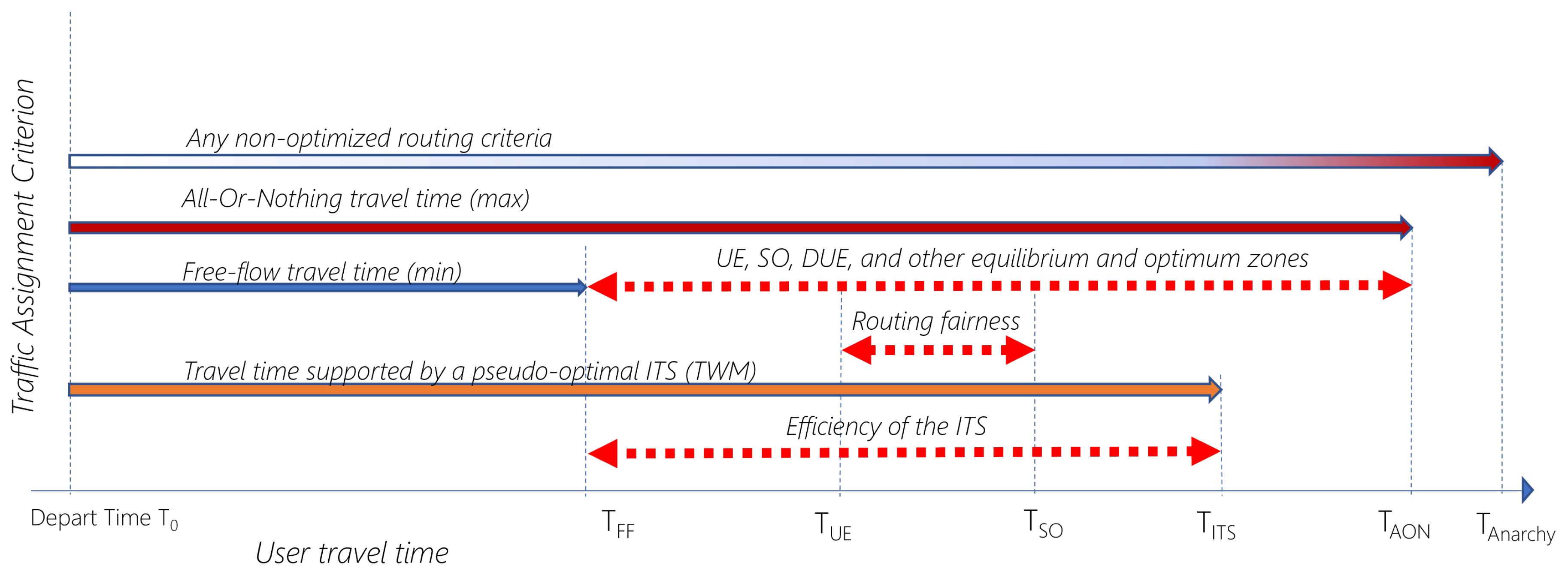
• Free-flow: vehicles use one optimal route and are calculated with basic link costs (1). Though an unreal scenario, it provides a lower bound for routing travel times.
• All-or-nothing: vehicles just use one route and consider link occupancy-costs (3). It is also an unreal scenario, but it delivers a reasonable higher bound in the case of optimal routing.
• System Optimum estimation strategies such as CAM, MSA or LP.

Our work relates to these previous studies in the flow-oriented and GA approaches used to solve the optimal process, though it has significant differences: (a) instead of distributing KSP routes, it uses multi-maps TWM that allows a feasible implementation for traffic routing having the benefits described in [8]; (b) path flows are defined as an abstraction of the O/D+KSP-based routing; (c) path flows determine a bonus-malus strategy encouraging the use of specific routes; (d) individual self-routing is possible using the TWM received without a central routing server; (e) the proposed GA algorithms are more straightforward as they do not use a per-vehicle optimization but a per-path flow basis: only traffic demand matrices are required instead of knowing individual trips in advance.

3. Traffic Multi-Maps Generation Based on Disjoint Path Flows

This section provides the TWM model formulation for map optimization, generation, assignment, and distribution strategies. The TWM model was first outlined in [8]. This paper extends the model to include Dj-kSP for TWM generation and optimal distribution. We rely on the recent multi-pass polynomial time algorithm and its ESX-C heuristic implementation described by Chondrogiannis et al. in [16], considering metrics and edge selection criteria and adding new ones to the original paper.

3.1. Traffic Model

The topological traffic representation of the urban network $\Theta$ is described by a graph $\Theta =G(N,E)$ formed by N nodes $\{{\eta }_n$} and E edges (links) $\left\{{ϵ}_e\right\}$ that connect them. The edge ${ϵ}_e$ connects the nodes ${\eta }_i$ and ${\eta }_j$, ${ϵ}_e=({\eta }_i,{\eta }_j)$, with a weight ${\omega }_e$. Edge weight is the intrinsic minimum cost of traversing it. It depends on physical and logical edge attributes, such as edge length $l_e$, edge max speed $s_e$, and edge tolls ${\tau }_e$. Edge weight is calculated considering the edge free-flow travel time $t_e^{FF}\left(x_e\right)$ (1) with no tolls where the vehicle assumes that it is the only user of the link [5].

$${\omega }_e=t_e^{FF}\left(x_e\right)=\frac{l_e}{s_e}$$

(1)

Traffic demand is composed of V vehicles $\left[v_a\right]$ that make trips between origin and destination nodes (O/D). The D unique O/D pairs in the demand form traffic commodities. Traffic flow $x^d$ is formed by the vehicles that belong to the same commodity $\mathrm{d}$, that is, moving from the same source node ${\eta }_i$ to the destination node ${\eta }_j$. Sources and destinations may refer to physical network nodes, traffic area zones, or traffic centroids. Total traffic flow (demand) in the network is $X=\left\{x^d\right\},\forall d\in D$.

Traffic flow $x^d$ may be routed through any of the $P^d$ feasible paths in the network connecting the source node ${\eta }_i$ to the destination node ${\eta }_j$. Any path $p_i^d\in P^d$ is an ordered sequence of connected edges with no loops. Traffic routing selects either statically or dynamically, some of these paths $\left\{p_i^d\right\}$ and allocate part of flow $x_i^d\in x^d$ to each path $p_i^d$, so that $\sum \left\{x_i^d\right\}=x^d$.

From the edge perspective, the traffic flow $x_e$ that traverses an edge ${ϵ}_e$ is formed by the traffic contribution of all the paths that traverse this edge (2).

$$x_e=\sum {\left\{x_i^d\right\}}_{\forall {ϵ}_e\in \left\{p_i^d\right\}}$$

(2)

The travel time $t_e\left(x_e\right)$ to traverse edge ${ϵ}_e$ depends highly on this traversing flow and is expressed by a volume-delay function $\Psi$ (VDF). The American Bureau of Public Roads (BPR) [64] defined VDF models to reflect the impact of edge occupancy being (3) the most widely used, where $W_e$ is the link capacity [11] and $\alpha$ and $\beta$ are predefined constants (typical values of $\alpha =0.15$ and $\beta =4.0$). This BPR link-cost model is widely used as a basis for traffic assignment.

$$t_e\left(x_e\right)={\omega }_e{(1+\alpha \frac{x_e}{W_e})}^{\beta }$$

(3)

Cost $c_e$ of an edge includes both the travel time and the eventual tolls ${\tau }_e$ that apply to the edge (4). Also, the free-flow cost of the edge is considered $c_e^{FF}$.

$$c_e=t_e\left(x_e\right)+{\tau }_e,\forall {ϵ}_e\in p_i^d$$

(4)

$$c_e^{FF}={\omega }_e+{\tau }_e,\forall {ϵ}_e\in p_i^d$$

(5)

Travel time $t_i^d$ over path $p_i^d$ is formed by the aggregation of the travel time at all the traversed edges (6):

$$t_i^d=\sum t_e\left(x_e\right),\forall {ϵ}_e\in p_i^d$$

(6)

The generalized cost model of a path $c_i^d$ considers both the travel time and the possible tolls associated with the edges that are included (7) as described in [25].

$$c_i^d=\sum c_e=\sum t_e\left(x_e\right)+\sum {\tau }_e,\forall {ϵ}_e\in p_i^d$$

(7)

We refer to the free-flow cost as $ff{c}_i^d$ (8).

$$ff{c}_i^d=\sum {\omega }_e+\sum {\tau }_e,\forall {ϵ}_e\in p_i^d$$

(8)

Route calculation is a complex process executed by the routing agents, which may be located either in the vehicle or in a remote ITS framework. Each routing agent ${\upsilon }_a$ calculates the best route to use for a trip of a commodity in terms of minimal route cost. This calculus is made for every trip and depends on the routing algorithm $\mathbb{R}$, the origin and destination nodes (commodity $\mathrm{d}$); the network map that it uses ${\mu }_a$; and the current traffic status and load in the network. It is measured as edge occupancy (or traffic density) $\left[{\rho }_e\right]$ [62]. The routing agent ${\upsilon }_a$ chooses a single path between all the paths $\left\{p_i^d\right\}\in P^d$ that will be referred as route ${\mathrm{r}}_{\mathrm{a}}$ for simplicity ($r_a=\left[p_i^d\right]$). Routing functions implement criteria such as bounded rationality or selfish behaviors [7,65] to implement traffic equilibrium principles at the user and system levels. Traffic assignment relies on these routing functions and how equilibrium conditions are applied.

Other valuable metrics associated with the route $r_a$ are the route length $L_a$, the number of traversed edges $E_a$, and the number of traversed nodes $N_a$.

Any routing agents ${\upsilon }_a$ and ${\upsilon }_b$ belonging to the same flow $x^d$ may select different routes. According to this, the traffic flow $x^d$ can be divided in sub-flows $\left\{x_i^d\right\}$ called path flows, containing each one of the vehicles that have selected the same route (9):

$$x^d=\left\{x_i^d\right\},\forall v_a,v_b\in x_i^d,r_a=r_b$$

(9)

Recent activity-based traffic models (ABM) [44] consider individual utility functions and driving constraints. The vehicles may also be grouped in Q sets called fleets that reflect their common requirements, such as electric cars, regular buses, scholar transport, diesel cars, etc. Traffic flows $X=\left\{x^q\right\},\forall q\in Q$ are also classified depending on the activity model.

Table 1. Traffic flow decomposition for five commodities and three fleets.

Commodities
Fleets		d${}_1$	d${}_2$	d${}_3$	d${}_4$	d${}_5$
	q${}_1$	$x^{1,1}$	$x^{1,2}$	$x^{1,3}$	$x^{1,4}$	$x^{1,5}$
	q${}_2$	$x^{2,1}$	$x^{2,2}$	$x^{2,3}$	$x^{2,4}$	$x^{2,5}$
	q${}_3$	$x^{3,1}$	$x^{3,2}$	$x^{3,3}$	$x^{3,4}$	$x^{3,5}$
	q${}_4$	$x^{4,1}$	$x^{4,2}$	$x^{4,3}$	$x^{4,4}$	$x^{4,5}$

shows an example of traffic flow decomposition for five commodities and   three fleets.

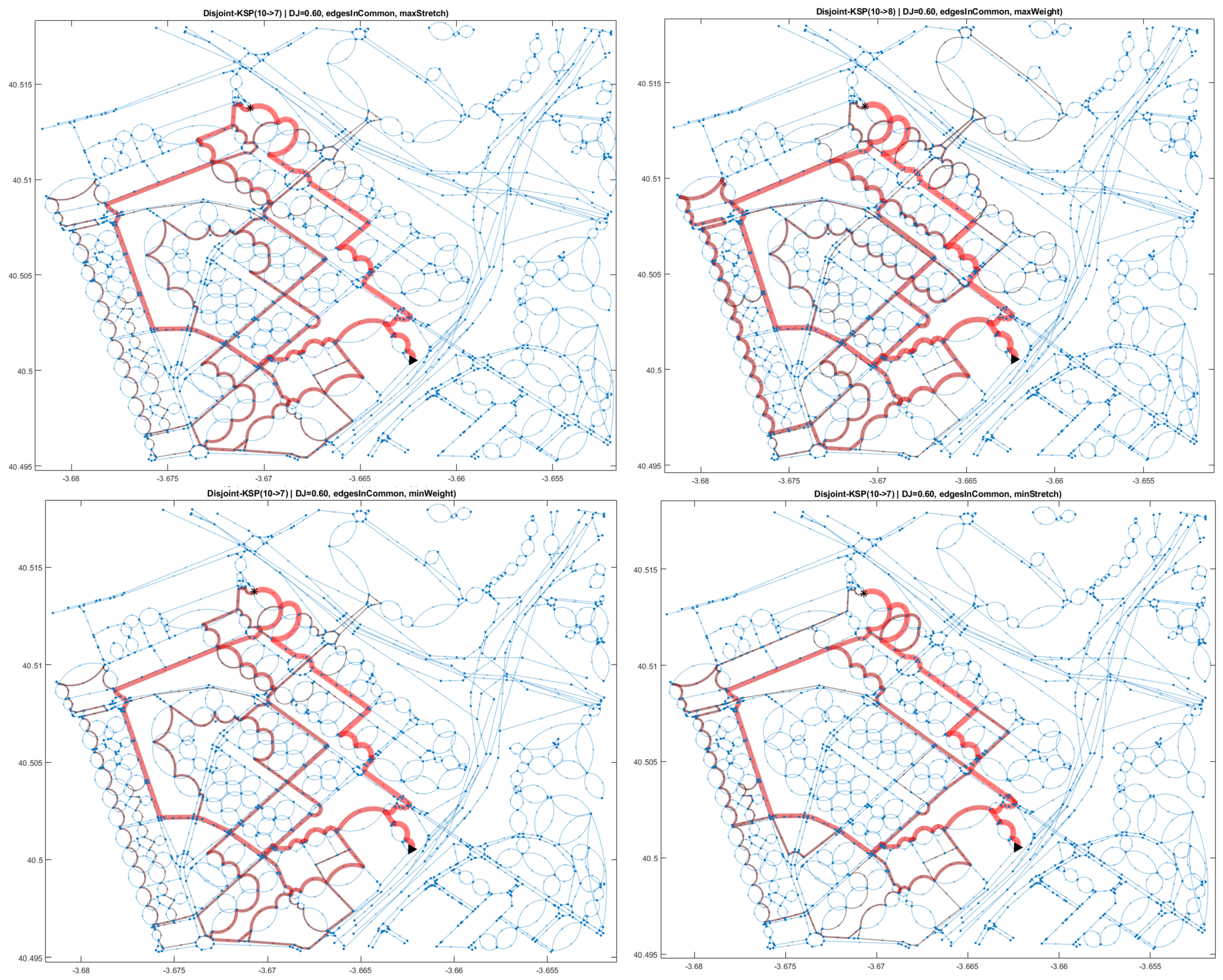
3.2. Semi-Disjoint K-Shortest Paths

When considering all the possible paths available for a commodity, it is necessary to analyze the disjoint level between them. If the first K shortest paths are selected, only one or two links may vary between them. It will cause congestion on some shared links when alternative routes are distributed to the flow. When designing traffic balancing, generating the best route alternatives and route variety is necessary.

$$Dj{C}_n=1-Si{m}_n$$

(10)

Disjoint level criteria $Dj{C}_n$ between two routes ${\mathrm{r}}_{\mathrm{a}}$ and ${\mathrm{r}}_{\mathrm{b}}$ is the inverse of their similarity $Si{m}_n$ (10). Complete disjointed paths a very restrictive constraint, so they is usually considered a partial path disjoint level, assuming a minimum disjoint level threshold $\varphi$. For instance, when a threshold $\varphi =0.6$ is used, any found paths must have at least a 60% difference, considering the similarity criteria selected. Different similarity criteria can be used:

• Edge-cost similarity (11) is the most used term (often simplified as “similarity”) and is measured as the ratio of accumulated cost from edges in common between ${\mathrm{r}}_{\mathrm{a}}$ and ${\mathrm{r}}_{\mathrm{b}}$ versus the minimum cost of the whole routes ${\mathrm{r}}_{\mathrm{a}}$ or ${\mathrm{r}}_{\mathrm{b}}$ [16]:

$$Si{m}_{EC}({\mathrm{r}}_{\mathrm{a}},{\mathrm{r}}_{\mathrm{b}})=\frac{\sum {\mathrm{c}}_{\mathrm{e}}^{\mathrm{FF}}}{\min \{{\mathrm{ffc}}_{\mathrm{a}}^{\mathrm{d}},{\mathrm{ffc}}_{\mathrm{b}}^{\mathrm{d}}\}},\forall {ϵ}_e\in r_a\cap r_b$$

(11)

• In Common-Edges similarity (12), ratio of the number of edges in common between both routes ${\mathrm{r}}_{\mathrm{a}}$ or ${\mathrm{r}}_{\mathrm{b}}$ versus the minimum number of links in both routes:

$$Si{m}_{EiC}({\mathrm{r}}_{\mathrm{a}},{\mathrm{r}}_{\mathrm{b}})=\frac{\mathrm{count}\left({\mathrm{ffl}}_{\mathrm{e}}\right)}{\min \{{\mathrm{E}}_{\mathrm{a}},{\mathrm{E}}_{\mathrm{b}}\}},\forall {ϵ}_e\in r_a\cap r_b$$

(12)

• Route-length similarity (13), differential route length ratio between the two routes ${\mathrm{r}}_{\mathrm{a}}$ and ${\mathrm{r}}_{\mathrm{b}}$ considering the minimum length of both routes, as it is considered in CSO [35]:

$$Si{m}_{RL}({\mathrm{r}}_{\mathrm{a}},{\mathrm{r}}_{\mathrm{b}})=\frac{\mathrm{abs}({\mathrm{L}}_{\mathrm{a}}-{\mathrm{L}}_{\mathrm{b}})}{\min \{{\mathrm{L}}_{\mathrm{a}},{\mathrm{L}}_{\mathrm{b}}\}}$$

(13)

• Route-cost similarity (14), differential route cost ratio between the two routes ${\mathrm{r}}_{\mathrm{a}}$ and ${\mathrm{r}}_{\mathrm{b}}$ considering the minimum cost of both routes:

$$Si{m}_{RC}({\mathrm{r}}_{\mathrm{a}},{\mathrm{r}}_{\mathrm{b}})=\frac{\mathrm{abs}({\mathrm{ffc}}_{\mathrm{a}}^{\mathrm{d}}-{\mathrm{ffc}}_{\mathrm{b}}^{\mathrm{d}})}{\min \{{\mathrm{ffc}}_{\mathrm{a}}^{\mathrm{d}},{\mathrm{ffc}}_{\mathrm{b}}^{\mathrm{d}}\}}$$

(14)

• Route-links number similarity (15), differential number of links ratio between the two routes ${\mathrm{r}}_{\mathrm{a}}$ and ${\mathrm{r}}_{\mathrm{b}}$ considering the minimum number of links in both routes:

$$Si{m}_{RN}({\mathrm{r}}_{\mathrm{a}},{\mathrm{r}}_{\mathrm{b}})=\frac{\mathrm{abs}({\mathrm{E}}_{\mathrm{a}}-{\mathrm{E}}_{\mathrm{b}})}{\min \{{\mathrm{E}}_{\mathrm{a}},{\mathrm{E}}_{\mathrm{b}}\}}$$

(15)

The k-Shortest Paths with Limited Overlap (kSPwLO) problem for a given commodity d is a weak NP-hard task that cannot be afforded by extensive searching over all the paths $\left\{p_i^d\right\}\in P^d$, as it grows exponentially [55]. There are exact algorithms to solve kSPwLO, but they require intense individual shortest-path processing (using Dijkstra or similar algorithms). In general, it is solved by a get_DjKSP procedure (16) that receives as inputs the traffic network $\Theta$, the commodity d (origin-destination pair), the routing algorithm to compute shortest paths $\delta$, the number of paths to find K and the minimal disjoint level threshold between paths $\varphi$. We use the Dijkstra algorithm for convenience [66]. However, other strategies may be used for the path flow calculus such as A*, or hyper-paths [62,67,68,69].

$$\begin{array}{cc}\hfill get\_DjKSP& :\Theta ,d,\delta ,K,\varphi ,Dj{C}_n,DjER{C}_n)\to \left\{r_i^d\right\}\hfill \\ \hfill & \left\{r_i^d\right\}\subset \left\{p_i^d\right\}\hfill \end{array}$$

(16)

Performance-oriented heuristic algorithms provide good enough solutions, such as the ESX-C proposed by Chondrogiannis [55]. It uses a heap of shortest paths that is iteratively incremented by recalculating a new shortest path (SP) while removing selected edges from the paths in the heap. A new SP is added to the heap when it fits the disjoint level criterion chosen. The algorithm loops until the Dj-kSP is set or no more SP can be found, and it returns the $\left\{r_i^d\right\}\subset \left\{p_i^d\right\}$ Dj-kSP.

Sometimes it is not possible to find precisely K disjoint paths that fulfill the disjoint level requirement for the $x^d$ traffic flow, so only the $K^{\ast }<K$ found paths can be used. We use the ESX-C algorithm for our purposes implemented by the $get\_DjKS{P}_{ESX-C}$ procedure. The count of all the returned Dj-kSP path flows is referred to as $numPF=count(\cup \left\{r_i^d\right\})$, and it is widely used in the optimization process.

Two main factors determine the selected Dj-kSP set: (a) the similarity criterion $Dj{C}_n$ used, and (b) the edge removal criteria at each iteration. Edge removal criterion $DjER{C}_n$ may be applied to the edge removal function to solve different traffic situations:

• Smallest/largest free-flow edge weight $c_e^{FF}$, $DjER{C}_{minW/maxW}$. If the MaxW is selected, the algorithm quickly selects highly disjoint paths though similar weighted paths are not considered. On the other hand, MinW enables a detailed full-scan approach.
• Minimum/maximum stretch, $DjER{C}_{minS/maxS}$, where stretch relates to the relative weight link contribution to the shortest path.
• Least/most local shortest paths, $DjER{C}_{minP/maxP}$ considering the amount of shortest paths that include an edge.

We consider the $\left\{r_i^d\right\}$ Dj-kSP as the alternative paths that any vehicle in the flow should consider for its trip in the traffic assignment problem. In this case, the $\left\{x_i^d\right\}$ path  flows will be directly affected by these $\left\{r_i^d\right\}$ routes. It is important to note that our model does not impose that vehicles must strictly follow these routes. The $\left\{r_i^d\right\}$ routes are used by the TWM generation algorithm to create the TWM maps, which will be selectively distributed to the vehicles.

3.3. TWM Model

A multi-map TWM, $\left[{\mu }_m\right]$, is a collection of M cost-weighted views (maps) of the traffic network $\Theta$, which the traffic groups in the network can use. Each map ${\mu }_m$ is a representation of the traffic network $\Theta$ (the m view), which complements the network map $\Theta$ with an additional set of link-weights and time constraints ${\mu }_m=\{\left[{\beta }_e^m\right],{\Gamma }_m\}$.

The Listing 1 shows the map appearance for the open source microscopic traffic simulation environment “Simulation of Urban MObility” (hereafter, SUMO) [70].

Listing 1. A ${\mu }_{002}$ map example showing edge weights and time validity intervals for the SUMO framework.

<twm id=“002”   mapName=“Madrid–LasTablas”   format=“sumo_1”   version=“1.0”>   <validity begin=“0” end=“2000” id=“time_001”>    <edge id=“NodeA_NodeB” weight=“1.871288”/>    <edge id=“NodeA_NodeC” weight=“2.508750”/>    <edge id=“NodeA_NodeD” weight=“1.918288”/>    ...    <edge id=“NodeM_NodeJ” weight=“2.470722”/>    <edge id=“NodeM_NodeL” weight=“2.176508”/>   </validity>   <validity begin=“2001” end=“4500” id=“time_002”>    <edge id=“NodeA_NodeB” weight=“1.871288”/>    <edge id=“NodeA_NodeC” weight=“3.882523”/>    <edge id=“NodeA_NodeD” weight=“2.640266”/>    ...    <edge id=“NodeM_NodeJ” weight=“2.730023”/>    <edge id=“NodeM_NodeL” weight=“2.176508”/>   </validity> </twm>

The TWM generation function $\Pi$ (17) provides the $\left[{\mu }_m\right]$ network views, taking as input (a) the network topology; (b) the Q traffic groups (fleets) that use the network; (c) the existing time-constraints $\left[{\Gamma }_m\right]$ for usage; and (d) network traffic status data $\Phi$. Time constraints $\left[{\Gamma }_m\right]$ consider both periodic-scheduled constraints (i.e., based on traffic restrictions, scholar times, commercial times, or similar) and event-based time constraints (i.e., road works, public events, road incidents, and others).

$$\begin{array}{cc}\hfill \Pi & :\Theta ,Q,\left[{\Gamma }_m\right],\Phi \to \left[{\mu }_m\right]\hfill \\ \hfill & {\mu }_m=\{\left[{\beta }_e^m\right],{\Gamma }_m\}\hfill \end{array}$$

(17)

Some routing agents may not use the TWM mechanism due to different causes: they are not part of the traffic groups that receive TWM, the TWM is not received on time, or they decline using TWM for their trip. They use the weights $\left[w_e\right]$ corresponding to the original physical map. We define the adherence factor $\psi$ (18) as the fraction of routing agents ${\left[{\upsilon }_a\right]}_{TWM}$ that are using it. We use $\psi$ to compare different TWM adoption scenarios.

$$\psi =\frac{\sum {\left[{\upsilon }_a\right]}_{TWM}}{\sum \left[{\upsilon }_a\right]}$$

(18)

3.4. TWM Weights Generation Based on Dj-kSP

The TWM generation function $\Pi$ needs to be modified as ${\Pi }_{DjkSP}$ (19) to create weight maps that encourage usage of the selected Dj-kSP routes $\left\{r_i^d\right\}$. To achieve this, we create the traffic groups Q according to the different Dj-kSP $\left\{r_i^d\right\}$ and generate a TWM map $\left[{\mu }_i^d\right]$. The use of a specific map with promoted edge weights induces the creation of the sub-flows $\left\{x_i^d\right\}$.

$$\begin{array}{cc}\hfill {\Pi }_{DjkSP}& :\Theta ,\left[{\Gamma }_m\right],\Phi ,\left\{r_i^d\right\},{\rm Y}\to \left[{\mu }_i^d\right]\hfill \\ \hfill & {\mu }_i^d=\{\left[{\beta }_e^{d,i}\right],{\Gamma }_m\}\hfill \end{array}$$

(19)

Each map ${\mu }_m$ is obtained by applying a transformation function ${\rm Y}$ to the weight of the edges, which are part of the Dj-kSP $r_i^d$. The most basic transformation function ${{\rm Y}}_{Lin}$ is the linear scaling by a constant factor ${\alpha }^{ϵ}$ to the original edge weight to decrease its weight and force the edges to be selected during the trip routing process.

$${{\rm Y}}_{Lin}:\Theta ,r_i^d,{\alpha }^{ϵ}\to \left[{\beta }_e^{d,i}\right]=\left[w_e\right]\ast {\alpha }^{ϵ}$$

(20)

The linear transformation does not assure that the selected path flow $r_i^d$ strictly has a path with lower cost than the best shortest path, unless an $\alpha$ factor is carefully selected. The ${{\rm Y}}_{Stretch}$ strategy is defined in (21) to solve it, where each map ${\mu }_m$ uses a different ${\alpha }_m$ depending on the global scaling factor ${\alpha }^{ϵ}$ and the relative cost influence (stretch) of the path flow $r_i^d$ over the total path flows $\left\{r_i^d\right\}$ available for the same flow. It is calculated using the free-flow total costs $ff{c}_i^d$.

$$\begin{array}{cc}\hfill {{\rm Y}}_{Stretch}& :\Theta ,r_i^d,\left[ff{c}_i^d\right],{\alpha }^{ϵ}\to \left[{\beta }_e^{d,i}\right]=\left[{\omega }_e\right]\ast {\alpha }_m,\forall ϵ\in \left\{r_i^d\right\}\hfill \\ \hfill & {\alpha }_m={\alpha }^{ϵ}\ast \frac{min\left(ff{c}_i^d\right)}{ff{c}_m^d}\hfill \end{array}$$

(21)

For instance, if we consider the flows $\{x_1,x_2,x_3\}$ with the corresponding path flows $\{\left\{r_{11},r_{12},r_{13},r_{14}\right\},\left\{r_{21},r_{22},r_{23},r_{24}\right\},\left\{r_{31},r_{32}\right\}\}$,

Table 2. Example of ${\alpha }_m$ values based on their path cost with ${\alpha }^{ϵ}=0.5$ factor.

Flow	Sub-Flow	Path Flow ${\mathit{r}}_{\mathit{i}}^{\mathit{d}}$	${\mathit{c}}_{\mathit{i}}^{\mathit{d}}$	${\mathit{\alpha }}_{\mathit{m}}$
$x_1$	$x_{11}$	$r_{11}$	1	0.5
	$x_{12}$	$r_{12}$	3	0.17
	$x_{13}$	$r_{13}$	5	0.10
	$x_{14}$	$r_{14}$	7	0.07
$x_2$	$x_{21}$	$r_{21}$	2	0.5
	$x_{22}$	$r_{22}$	4	0.25
	$x_{23}$	$r_{23}$	6	0.17
	$x_{24}$	$r_{24}$	8	0.13
$x_3$	$x_{31}$	$r_{31}$	5	0.5
	$x_{32}$	$r_{32}$	10	0.25

shows the ${\alpha }_m$ values for the path flows according to their path cost (free-flow cost) and an ${\alpha }^{ϵ}=0.5$ factor.

Using TWM for vehicle routing expands the concept of routing paths to the routing area. In urban traffic networks, a particular routing path may have multiple small alternatives through the closest crossings and streets, which minimally impacts global path costs. They may provide efficient solutions when an edge becomes congested or suffers an incident. We can also lighten these minor path variations around the nodes ${\left\{{\eta }_x\right\}}_i^d$ contained in the path flow $r_i^d$ so that the routing agent can consider them as a suitable alternative while searching for the best path considering the edge occupancy.

The mechanism to generate the TWM for the routing area around the path flow $r_i^d$ is straightforward and described by (22):

$$\begin{array}{cc}\hfill {{\rm Y}}_{Stretch\_Area}& :\Theta ,r_i^d,c_i^d,{\alpha }^{ϵ},R,{\alpha }^1\to \left[{\beta }_e^{d,i}\right]=\left[{\omega }_e\right]\ast {\alpha }_m^{\ast }\hfill \\ \hfill {\alpha }_m^{\ast }={\alpha }_m& ,\forall ϵ\in \left\{r_i^d\right\}\hfill \\ \hfill {\alpha }_m^{\ast }={\alpha }_m\ast {\alpha }^R& ,\forall ϵ\in \Theta ,dist({\eta }_a,{\eta }_b)\in [1,R],\hfill \\ \hfill & {\eta }_a\in \left\{r_i^d\right\},{\eta }_b\in ϵ\hfill \end{array}$$

(22)

First, we select all the edges ${\left\{{ϵ}_e\right\}}_i^d$ connecting the neighbor nodes at a distance R (proximity radius) from the ${\left\{{\eta }_x\right\}}_i^d$ nodes of the path flow, and then a new ${\alpha }_m^{\ast }$ factor is applied to them considering a new ${\alpha }^R$ penalty. Figure 3 illustrates this method with a synthetic traffic network and two completely disjoint path-flows.

The distance between two nodes $dist({\eta }_a,{\eta }_b)$ may be evaluated in diverse ways: as the number of hops (edges) that separate them or as the cost function between them. For simplicity, we will consider the number of hops between them.

The complete TWM generation is described in Algorithm 1.

When the routing agent uses the TWM map ${\mu }_i^d$ based on the path flow $r_i^d$, the route costs are calculated with the new edge weights. The occupancy/capacity link-cost model described by (3) evolves to (23).

$$t_e^{TWM}\left(x_e\right)={\beta }_e^{d,i}\ast {(1+\alpha \frac{x_e}{W_e})}^{\beta }$$

(23)

It is also possible to define an obvious ${{\rm Y}}_{Toll}$ strategy that adds/removes tolls to the generalized cost function in (7).

Algorithm 1 TWM generation algorithm based on Dj-kSP

Require:  traffic network $\Theta$, commodities D, shortest paths algorithm $\delta$, max SP K, disjoint level threshold $\varphi$, disjoint level criteria $Dis{j}_n$ and $DjER{C}_n$ as $C_1$ and $C_2$, alfa factors ${\alpha }^{ϵ}$ and ${\alpha }^R$, edge proximity radius R Ensure: TWM maps $\left[{\mu }_i^d\right]$ as $twm$   1: $twm\leftarrow \left(\right)$   2: for all (d in D) do {iterate over commodities}   3:  {Get Dj-kSP and their free-flow costs}   4:  {Use ESX-C or similar algorithm}   5:  $\left(r_i^d\right),\left(ff{c}_i^d\right)\leftarrow get\_DjKSP(\Theta ,d,\delta ,K,\varphi ,C_1,C_2)$   6:  $nr\leftarrow size\left(\left(r_i^d\right)\right)$   7:  $\mu \leftarrow array(nr,\Theta )$ {allocate maps}   8:  for all (r in $\left(r_i^d\right)$) do {weight the maps}   9:   $\mu \left(r\right)\leftarrow \Theta$ {assign the initial network} 10:   ${\alpha }_m\leftarrow {\alpha }^{ϵ}\ast \frac{min\left(ff{c}_i^d\right)}{ff{c}_r^d}$ 11:   for all ($ϵ$ in r) do {assign weights to path edges} 12:    $\mu \left(r\right)\left(ϵ\right).weight\leftarrow {\alpha }_m\ast \Theta \left(ϵ\right).weight$ 13:   end for 14:   $rEdges\leftarrow get\_surroundingEdges(\Theta ,r,R)$ 15:   for all ($ϵ$ in $rEdges$) do {assign weights to the R-closest edges} 16:    $\mu \left(r\right)\left(ϵ\right).weight\leftarrow {\alpha }_m\ast {\alpha }^R\ast \Theta \left(ϵ\right).weight$ 17:   end for 18:  end for 19:  $twm\leftarrow push(twm,{\mu }^d)$ 20: end for

4. Optimal TWM Assignment

Once the TWM maps have been designed favoring the different traffic flows according to their possible best disjoint routes, the question to be solved is what will be their best allocation to achieve the system’s optimum, measured as the minimum mean travel time.

Optimal distribution strategies minimize average travel time from a system-wide perspective. Different algorithms based on GA were preliminarily introduced in [12] for accomplishing this goal, applying two strategies: per vehicle optimal assignment (OTV) and per path flow optimal assignment with linearly constrained or unconstrained (LCTV/UCTV).

All of them use the mean travel time evaluation procedure $computeMTTS$ (24), which uses the network view ${\mu }_i$, the network occupancy is expressed as the trips (routes) assigned to each vehicle $\left\{p_i^d\right\}$, a reference to a volume-delay function $\Psi$ (VDF), and its specific VDF arguments ${\Psi }_{args}$. It computes the aggregated edge occupancy based on the individual routing decisions, which are then used for the VDF evaluation with the edge weight, the edge capacity, and the corresponding VDF arguments [5].

$$\begin{array}{cc}\hfill & computeMTTS:{\mu }_i,\left\{p_i^d\right\},\Psi ,{\Psi }_{args}\to mtts\hfill \end{array}$$

(24)

$$\begin{array}{cc}\hfill & x_e\leftarrow count\left(ϵ\right),\forall ϵ\in \left\{p_i^d\right\}\hfill \end{array}$$

(25)

$$\begin{array}{cc}\hfill & mtts\leftarrow mean(\Psi ({\mu }_i\left({\beta }_e^{d,i}\right),x_e,{\mu }_i\left(W_e\right),{\Psi }_{args}),\forall ϵ\in \left\{p_i^d\right\}\hfill \end{array}$$

(26)

As discussed in [12], OTV has significant drawbacks. First, the number of vehicles in the network directly influences the number of variables that need to be optimized (the chromosome size will shape the number of vehicles), leading to a demand for extensive computing resources that may be unaffordable even in small scenarios. Second, optimizing the microscopic assignment of TWM based on flows and path flows offers a macroscopic perspective of the traffic demand. As a result, it may not accurately represent traffic planning since it depends on specific trips.

Considering the assignment of maps per path flow, we may surpass the pointed limitations. In this approach, each sub-flow $x_i^d$ is assigned a fixed TWM map ${\mu }_i^d$. The challenge now lies in solving the number of vehicles assigned to each sub-flow, that is, how many vehicles will use each ${\mu }_i^d$ efficiently. The distribution is determined as a percentage of the traffic for every commodity d. Consequently, each vehicle will be assigned the appropriate path flow map.

The GA function generates the chromosome ${\aleph }_1$ with a $numPF$ size. Each value represents the percentage of vehicles from each flow allocated to a particular sub-flow $x_i^d$. Two constraints are applied to ensure the validity of the chromosome. First, $[0,1]$ normalization is enforced. Second, flow conservation is maintained, which means that the sum of all vehicle percentages belonging to the same flow must equal 1. Both constraints are directly incorporated into the GA algorithm.

The GA fitness function for LCTV is invoked during each population iteration to compute the mean travel time (MTTS). It receives the chromosome ${\aleph }_1$ to evaluate the VDF function $\Psi$, the physical network map ${\mu }_0$, the traffic flows $\left\{x_i^d\right\}$, the path flows $\left\{r_i^d\right\}$, and the TWM $\left[{\mu }_i\right]$.

The GA solver with linear constraints reduces the target population since it discards the individuals from the GA that do not fit them. This elimination of individuals evaluates the algorithm longer. It leads to worse results, as we will see in the case studies. The unconstrained solver UCTV applies the normalization step at the end of the process to the resulting values to compute the corresponding TWM distribution.

5. Materials and Methods

The experiments were developed using Matlab R23A on a Windows 11 system with an iCore7 2.10GHz processor and 64GB RAM.

The genetic algorithms utilized Matlab’s global optimization toolbox [10].

The resulting TWM maps are dumped in data files compatible with SUMO 1.18 [70].

The solutions use a plugin developed for TWM management through the TRACI interface at SUMO.

Each TWM allocation strategy involving a stochastic process was repeated 100 times for the GA execution and the random population adherence to achieve the necessary confidence intervals in the results presented. Experiments with 10, 20, 50, 50, 80, and 100 repetitions were carried out, all showing congruent and convergent results from the first values and very low dispersion of the results.

6. Results

To obtain the experimental results, we use the Madrid-Las Tablas district’s real urban traffic network, described in [34]. Different routing strategies are evaluated regarding MTTS and the effects of Dj-kSP and routing area variation are analyzed.

As pointed out in (16) and (19), multiple variations can be applied to generate the corresponding TWM maps:

• The number of K alternative paths considered for Dj-kSP. We vary on it, typically ranging between 3 and 10. Selecting a low K value will not create route variety, and using a higher number presumably is worthless as it will not find so many disjoint paths. Using a high K value has a significant performance penalty in the Dj-kSP algorithm with polynomial time complexity.
• The routing algorithm $\varphi$ is used to calculate the minimum cost route. In this work, we use the Dijkstra algorithm as it will not significantly affect the resulting maps. The routing algorithm performance affects the overall performance as the traffic assignment used during the optimization stage uses it extensively.
• The disjoint level criteria $Dj{C}_n$ used to evaluate the disjoint level of the paths. It is a traffic planning decision that conditions how routes are generated depending on the edge selection policy used. It is analyzed in the experimental section. This parameter also affects algorithm performance during the Dj-kSP calculation phase, as edge removal could take broader searches.
• The disjoint level threshold $\varphi$. We also vary it, with a typical value of 60%. This a traffic planning decision, where a high value of disjointness (>80%) probably will not produce the necessary variety of alternative routes, and a low value (<30%) will generate very overlapping routes. The combination of $\varphi$ and K directly affects the number of Dj-kSP and, consequently, the path flows to be obtained since there may not be enough alternative paths that meet the maximum overlap constraints.
• The similarity criterion (max/min Stretch, max/min Weight, max/min Crossing Paths) affects the performance of Dj-kSP calculation and the effectiveness of the routes found. Also, depending on the selected criterion, the ESX-C algorithm finds different paths or restricts the ones found. Our experiments and the findings described by [16] suggest using the maxStretch or the maxWeight edge-removal criteria as they lead to better assignment.
• The distance of surrounding nodes to the nodes of each path flow, to define the routing areas. It should be greater than 1 to find some routing alternative; a typical value ranges from 2 to 5 connected nodes. It is possible to use higher values, but the routing areas probably would overlap, losing the disjointness properties. It does not affect the algorithm’s performance.
• The different utility functions for the vehicle fleets. This item is not considered in the scope of this work.

The map assignment to the vehicles and the static traffic (route) assignment processes also have different variation alternatives:

• The adherence factor $\psi$ (18) of the vehicles using TWM.
• The own GA resolution parameters.

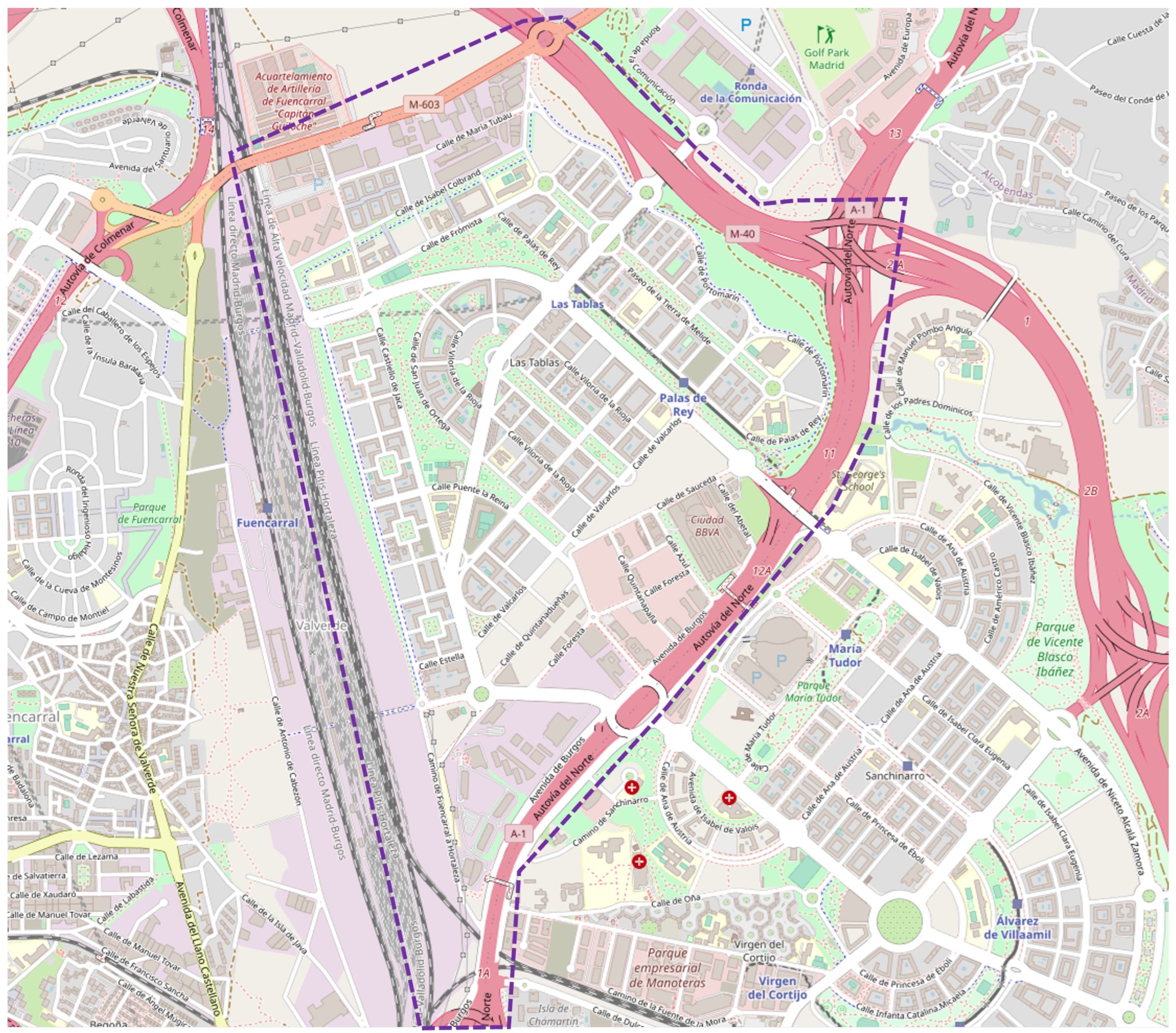
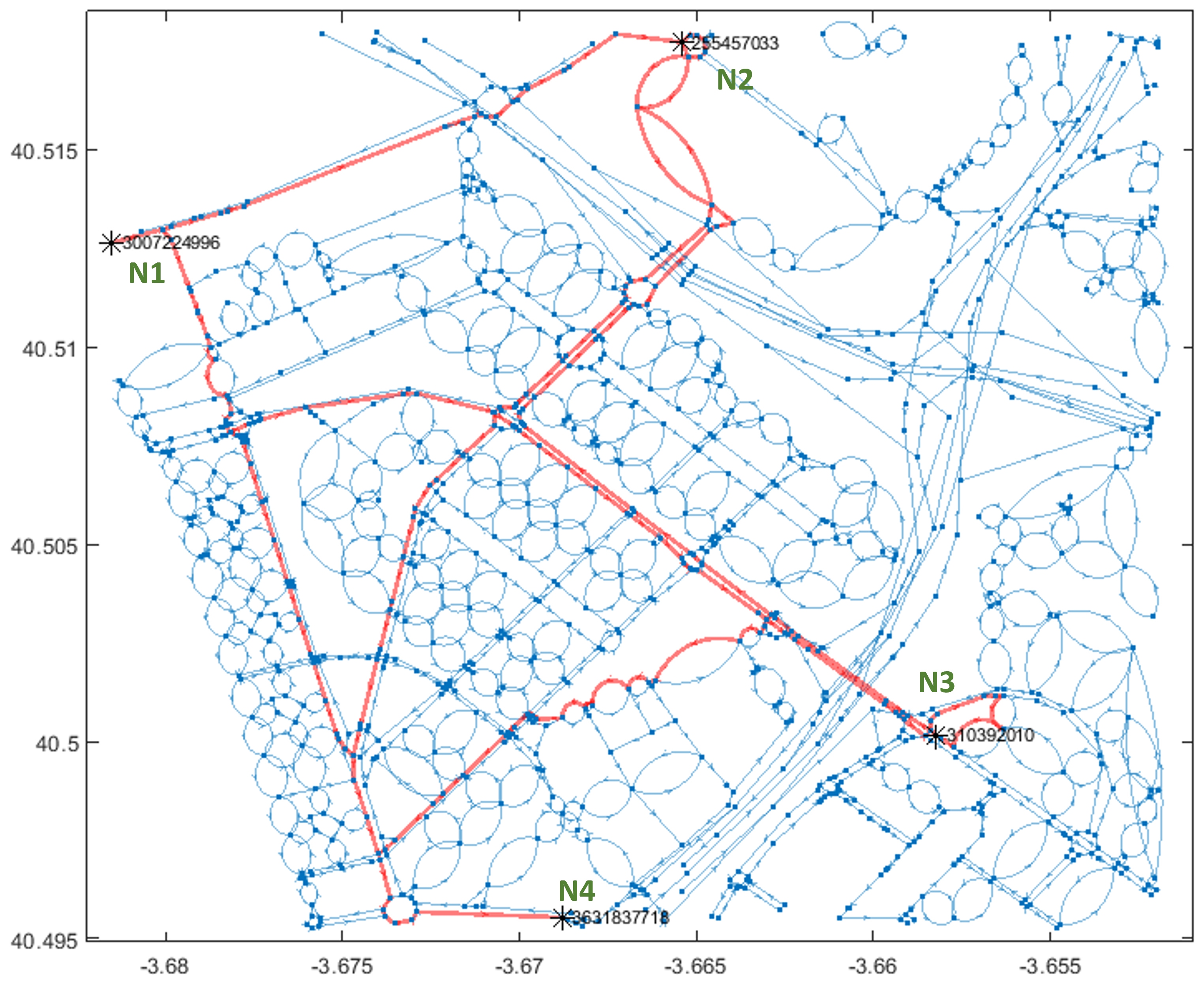
6.1. Madrid-Las Tablas Traffic Scenario (MLT)

This traffic scenario was first outlined in [34]. The traffic network is depicted in Figure 4 and Figure 5 and consists of 971 nodes and 1583 links covering one of the largest districts in Madrid, Spain. It spans over 24,300 hectares with approximately 43,000 residents plus a daily floating job population of around 38,000 office workers. The district also has major commercial and financial hubs, leading to significant traffic influx and outflow during business hours. Its borders are defined by major expressways to the north, south, and east, while railways block the western side. The scenario contains a synthetic traffic demand of 3500 vehicles generated to simulate congested areas across the network. It is divided into 7 flows of 500 vehicles each, as depicted in Figure 5 and

Table 3. Madrid-Las Tablas O/D Matrix.

Source/Destination	N1	N2	N3	N4
N1		500	500	500
N2			500	500
N3		500		500

.

Dj-kSP TWM Maps Generation

Due to the size, complexity, and variety of parameter combinations that generate the path flow sets for the MLT network, we will develop in-depth relevant experiments pointing to the significant variations around it. The reference experiment uses $K=6$ semi-disjoint paths with an index of $\varphi =0.6$ (there can only be a maximum of 40% overlap between paths) and a distance radius of $R=5$. We concentrate on the “Edge-Cost” $Dj{C}_n$ removal policy by affecting the fundamental criterion for creating TWMs, which are the weights of the edges.

Figure 6 illustrates the Dj-kSP obtained for the flow ($N3$→$N5$) using the disjoint criteria for edges in common, $Si{m}_{EiC}({\mathrm{r}}_{\mathrm{a}},{\mathrm{r}}_{\mathrm{b}})$, applying different edge removal policies ($DjER{C}_{maxW}$, $DjER{C}_{minW}$, $DjER{C}_{minS}$, $DjER{C}_{maxS}$). It is remarkable to observe that the ESX-C algorithm sometimes cannot find the target of K Dj-kSP with the applied disjoint level constraints (not enough paths that meet the requirements).

For instance, Dj-kSP process for the MLT scenario applying $Si{m}_{EiC}({\mathrm{r}}_{\mathrm{a}},{\mathrm{r}}_{\mathrm{b}})=60\%$ with $DjER{C}_{minW}$ and K = 6, will return only 17 path-flows. The same scenario with $Si{m}_{EiC}({\mathrm{r}}_{\mathrm{a}},{\mathrm{r}}_{\mathrm{b}})=30\%$ will return 41 path-flows.

6.2. TWM Assignment and Routing Strategies

Different scenarios are compared to check the effectiveness and quality of the solution proposed by TWM(Dj-kSP):

• Free-Flow and All-Or-Nothing to obtain the minimum and maximum assignment values as discussed in previous sections.
• The user equilibrium estimated solutions are provided by methods such as the cumulative, the successive averages, the Frank-Wolfe [5], and Wei [19]. Although they offer approximate theoretical values, they give us an insight into the actual quality of the solution offered by other strategies.
• Ideal routing solutions for MTTS in hypothetical scenarios that do not use TWM and, thus, no adherence to them is considered. They are included for:

  kSP(u)     

  When the vehicles use the most straightforward k-shortest paths (not considering disjoint level) for each flow and use a random uniform assignment under AON conditions. The scenario is unrealistic as it does not reflect the selfish behavior of the routing agents.

  kSP(f)      

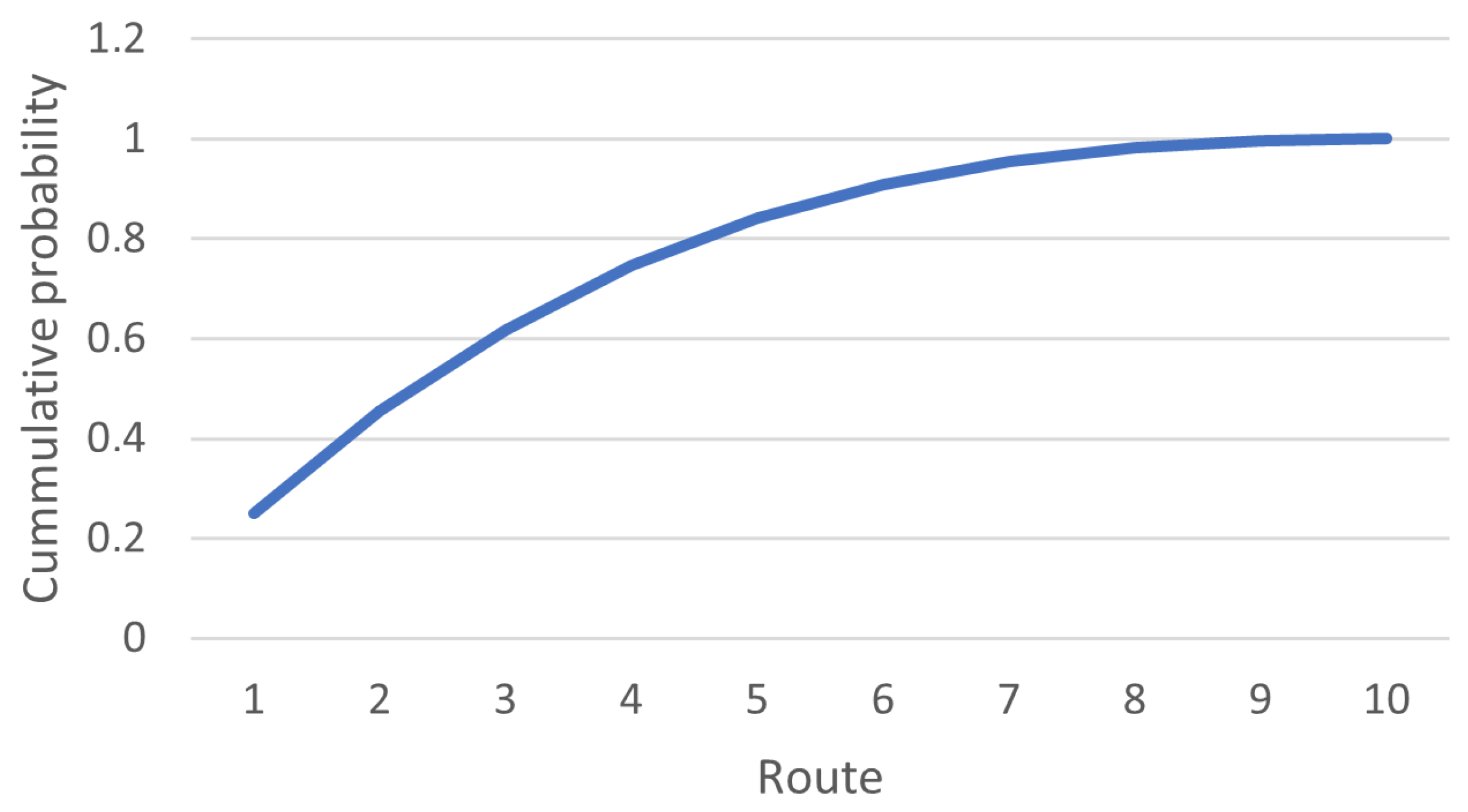
  When the vehicles use the simplest k-shortest paths (not considering disjoint level) for each flow and a random Fibonacci-based assignment for them shown in Figure 7. This Fibonacci series emulates a procedure to incrementally assign kSP routes to the vehicles.

  Dj-kSP(f)    

  When the vehicles directly use the Dj-kSP routes for each flow with the random Fibonacci-based assignment.

  Dj-kSP(opt)   

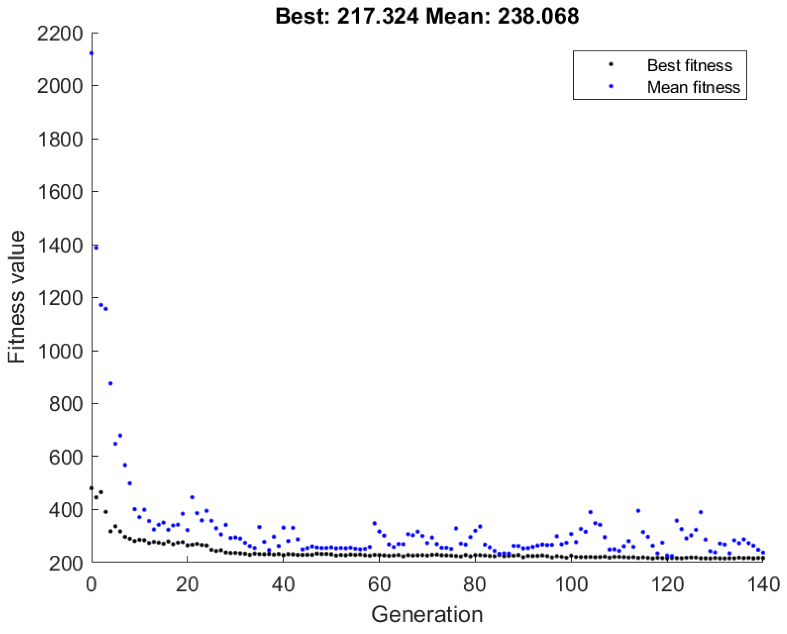
  When the vehicles directly use the Dj-kSP routes for each flow, calculating an optimal assignment. This optimal assignment is achieved using a GA engine.

• Usage of Dj-kSP-based TWM, based on different adherences $\psi$ in the routing agents.

  $\psi$-TWM(f)  

  When the vehicles use the TWM maps with a $\psi$ adherence ratio and a random distribution (uniform or Fibonacci) for assignment.

  $\psi$-TWM(opt) 

  When the vehicles use the TWM maps with a $\psi$ adherence ratio and an optimal assignment with UCTV algorithm. It is our main objective.

As pointed out before, some variations cannot be covered extensively in this paper, so we have selected the most relevant ones to illustrate how these parameters affect the TWM routing efficiency.

UCTV Parameterization

For the optimal assignment solutions, the UCTV genetic algorithm uses a ${\aleph }_1$ chromosome with $numPF$ genes, which will return a collection of $numPF$ values. They correspond to the volume of vehicles of each sub-flow which will receive the corresponding TWM map. $numPF$ depends on the disjoint level criteria and edge-discard criterion used, and of course, on the redundancy of feasible paths in the physical topology of the traffic network.

The UCTV-GA uses an initial population of $k_1\ast numPF$ individuals and $k_2\ast numPF$ generations. Using $k_1=5$, the algorithm’s convergence to the mean value is quickly achieved in all scenarios in $k_2⩽10$ generations. These values have been selected after multiple experiments using high values and analyzing how the algorithm converges. Gene values in the chromosomes are $[0,1]$ normalized. Selection applies a stochastic uniform strategy in every evolutionary step using an elite count of 5% of immutable individuals and selecting random individuals from uniformly distributed population buckets arranged linearly. Crossover is limited to a $k_3$ fraction of the genes, applying a $[0,1]$ normalized random scattered function. The crossover fraction applied is $k_3=0.8$. Mutation uses a zero-mean Gaussian operator with a 1-normalized scaling factor that shrinks its amplitude at every iteration of the algorithm by a factor or $\frac{g}{G_{max}}$ where g is the current generation of the algorithm and $G_{max}$ is the total number of generations.

Figure 8 shows UCTV genetic algorithm execution for the TWM(Dj-kSP) assignment, with 60% disjoint level, “Edge-costs” disjoint level policy, 6-kSP and minWeight edge discard. This scenario returns a $numPF=21$.

7. Discussion

Figure 9, Figure 10, Figure 11 and Figure 12 compare some scenario configurations and driver adherences. They have been created using Matlab’s boxplot diagram to display values dispersion between 2% and 75%, their 95% confidence interval, and the median value marked in red. The median is taken as a reference for comparison.

Free-Flow and All-Or-Nothing values are displayed as dotted lines as min/max bounds, together with the User Equilibrium estimated from the mean value of the approximate cumulative and successive averages, the Frank-Wolfe, and Wei-Linear-Programming methods. These lines allow for a quick comparison of the values obtained by the different map assignments and routing strategies for the static traffic assignment.

Figure 9 illustrates the comparative strategy for the 3-kSP, 60% Disjointed, Edge-cost policy with minWeight discard selection, showing the scenarios kSP(u), kSP(f), Dj-kSP(f), Dj-kSP(opt), and $\psi$-TWM(f) and $\psi$-TWM(opt) for different values of TWM driver adherences of [25%, 50%, 75%, 100%].

As we can observe, the direct assignment of k-shortest path routes to the vehicles (kSP and Dj-kSP) does not provide better results than the All-Or-Nothing approach: as the edge costs rise due to their occupancy, the kSP calculation is affected, so routing agents compute and select other different kSP considering the new VDF costs. They do not use a TWM map, so they consider just their plain original information. However, these are not realistic approaches since routing agents will not follow these expected kSPs under the free-flow assumption.

On the other hand, the optimal Dj-kSP assignment method provides a good understanding of the theoretical limits of the TWM-based method in case of a perfect adoption scenario ($\psi =100\%$). But it is neither a realistic approach as the routing agents are not supposed to take precisely the Dj-kSP unless a central ITS is used to provide routes to the vehicles and they follow them strictly.

Nevertheless, the TWM-based approaches consider that the routing agents freely use the promoted routing areas around the pre-calculated Dj-kSP coded in the TWM. They also take into account the VDF costs based on occupancy. As traffic is intrinsically diverted to promoted routing areas using the TWM, the links have lower occupancy, and therefore, VDF costs have a softer impact.

Table 4. MTTS Figures index.

Figure	Dj-kSP	Disjoint Criterion	$\mathit{\varphi }$	Edge Policy	Adherences	Comments
Figure 9	3	Edge costs	60%	minWeight	25%, 50%, 75%, 100%	Compare with kSP assignment
Figure 10	3	Edge costs	60%	maxStretch	25%, 50%, 75%, 100%
Figure 11	6	Edge costs	60%	maxWeight	25%, 50%, 75%, 100%
Figure 12	6	Edge costs	30%	maxStretch	25%, 50%, 75%, 100%

addresses the analysis scenarios.

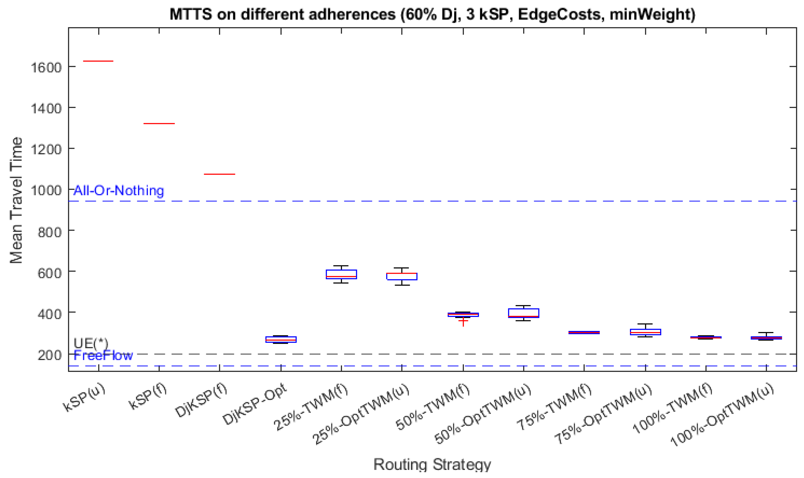
7.1. Effects of Driver’s Adherence to TWM

In our previous works [12,34], a driver’s adherence to TWM was already identified as a critical factor for TWM success, both in static assignment and in dynamic behavior using econometric models of utility functions and fuzzy logic.

The effectiveness and impact of Dj-kSP-based TWMs depend on the adherence factor $\psi$ as it is shown in Figure 9. Our experiments covered driver adhesion based on quartiles with $\psi =25\%,50\%,75\%,100\%$.

Even with low adherence of 25%, the traffic assignment using TWM significantly impacts the overall traffic scenario since the vehicles that use alternative paths relieve the most congested links (

Table 5. Number of routes obtained with different adherences.

Figure	Dj-kSP	Disjoint Criterion	$\mathit{\varphi }$	Edge Policy	Adherences
Figure 13	6	Edge costs	3	maxStretch	25%
Figure 14	6	Edge costs	3	maxStretch	50%
Figure 15	6	Edge costs	3	maxStretch	75%

). As the level of adherence increases, the impact on traffic assignment becomes greater, though not linearly, as the alternative paths also raise their occupation status, and their edge costs depend on their occupancy. In Figure 9 and Figure 10 we observe how 75% of drivers’ adherence approaches the minimal MTTS marked by Dj-kSP(opt). A complete adherence scenario hardly improves MTTS, or even worsen it, as in the case of maxWeight in Figure 11.

The effect of optimal TWM distribution depends on the number of path flows $numPF$, which in turn depends on the number of flows and the number of Dj-kSP in the product $F\ast K$. As can be seen from the diagrams, TWM(Dj-kSP) provides sufficient variety and diversity of routes for the flows so that the optimal distribution could be providing more improvement, making the approach much more interesting for its efficiency.

Figure 13, Figure 14 and Figure 15 show the route dispersion for the flows in three snapshots of concrete traffic assignments with different adherence levels of 25%, 50%, and 100%. These routes are assigned to the vehicles using the TWM map set considering the edge occupancy. In 25% adherence, few vehicles use the alternative routing with TWM, and therefore there is not a great variety of routes, obtaining 45 routes but with high usage in a few of them. The full adherence scenario induces disjoint paths that could be more optimal, obtaining 41 routes with dispersed usage. 50% adherence scenario shows how 48 routes are selected with high use.

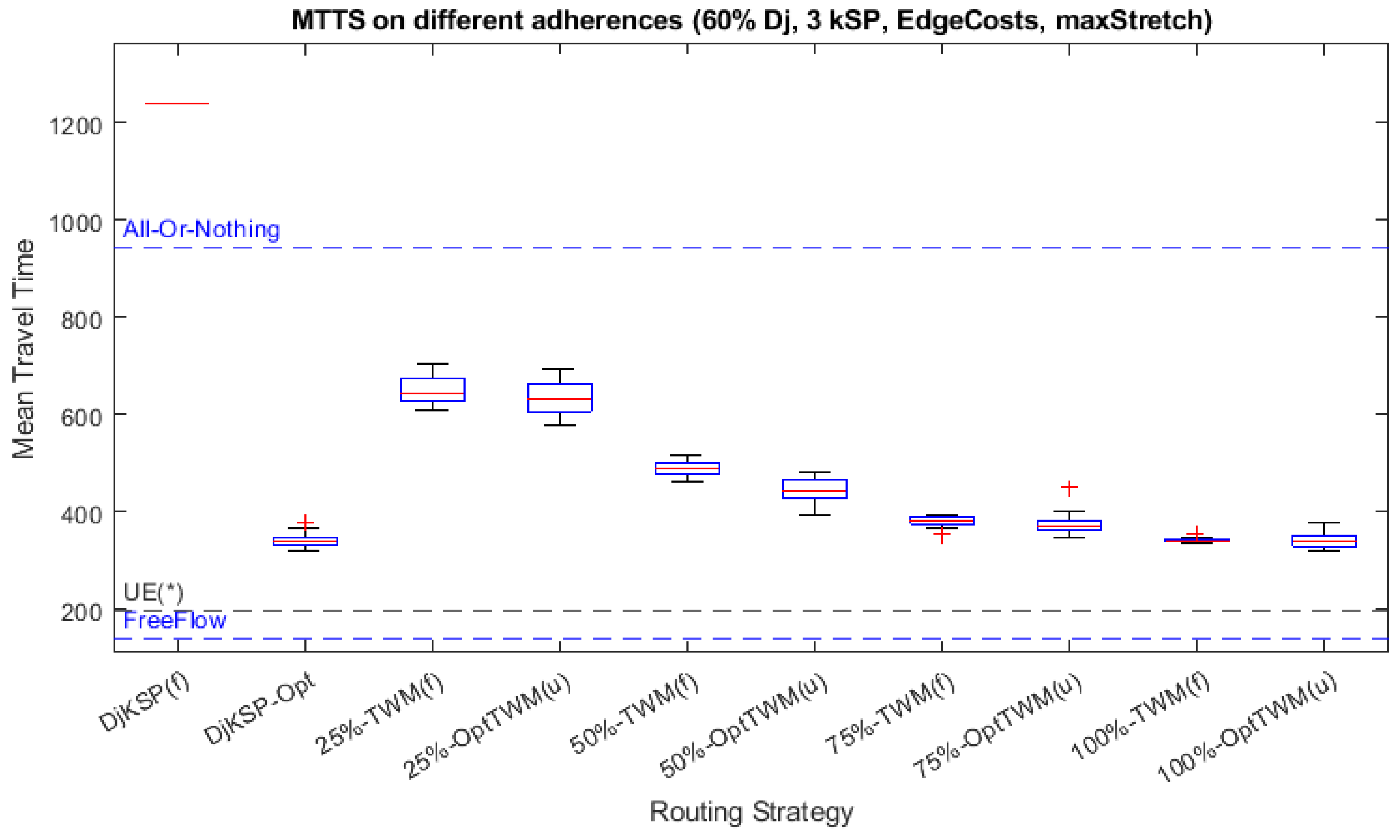
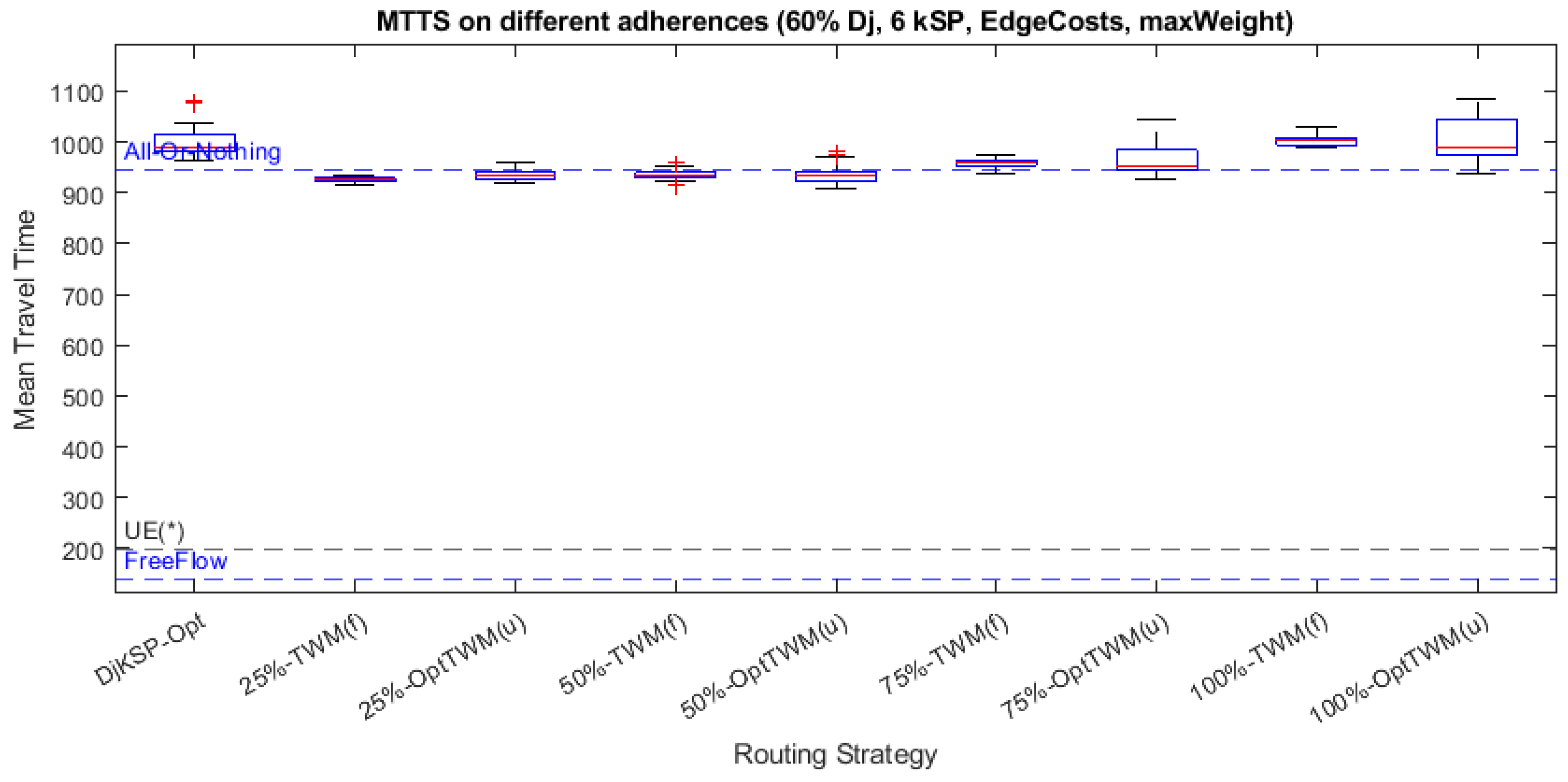
7.2. Effects of Edge Removal Criterion

If we compare the scenarios {minWeight with 3 Dj-kSP, 60% disjoint} and {maxWeight with 6 Dj-kSP, 60% disjoint}, we could affirm that having more path flows and using a policy that discards the edges with higher costs earlier, we would obtain a better traffic assignment. But it is not the case, as can be seen in Figure 9 and Figure 11, where we can see that the maxWeight edge removal policy provides bad results, even duplicating the number of Dj-kSP. The justification for this is that in the search for the Dj-kSP the edges with the most significant weight are eliminated, but this causes the incorporation of other edges with even greater weight. Let us remember that the starting point was using the shortest path. Vehicles will only accept the use of these Dj-kSP unless the occupancy of edges on the best routes increases their costs above the cost of the new route.

The minWeight policy provides the best results, replacing the edges with minimal costs for new alternatives with minimal costs in the disjoint paths. The maxStretch policy also provides reasonable solutions because we replace edges with a high relative impact on the path for others with a similar one.

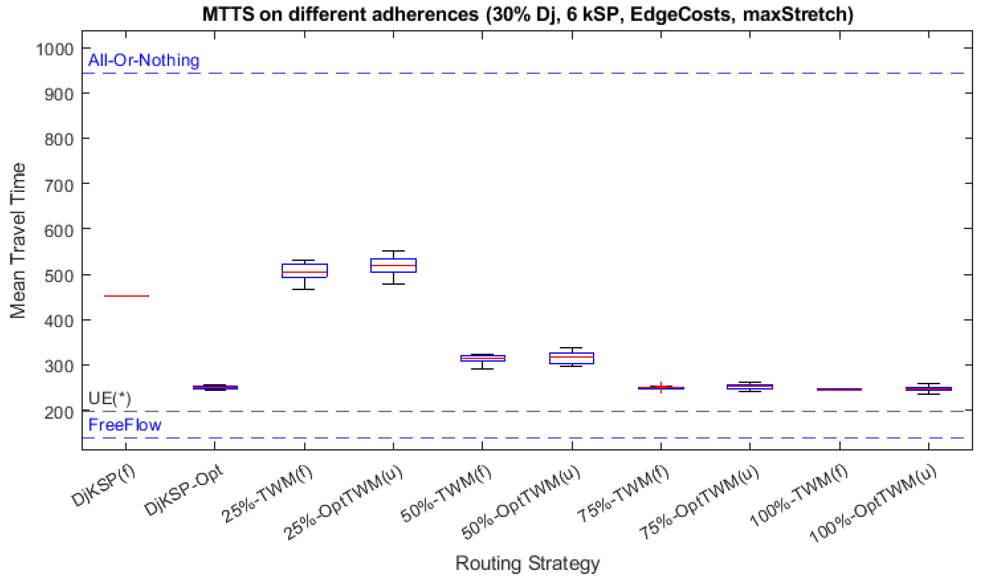
7.3. Effects of Disjoint Level Threshold

The use of very high levels of disjoint threshold has two main effects: a) restricting the number of disjoint routes, as it will depend on the topological connectivity of the traffic network. In the MLT network, the Dj-kSP calculation for 6 routes with minWeight and 60% disjoint level returns in some O/D tuples just 2 or 3 matching paths. If we lighten the disjoint constraint to 30%, we obtain 5 or even 6 paths, which provide the required path variety. These path flows are used to generate the TWM maps that will be used later for route selection by the routing agents.

8. Conclusions

Though TWM has yet to be deployed in real traffic scenarios, simulations show that using Traffic Weighted Multi-maps effectively creates alternative routes for traffic planning and assignment. The complexity of new ITS deployments requires extensive previous simulation. TWM management involves four main stages: map generation, map allocation, map distribution, and map adoption from a dynamic econometric utility perspective. They are compatible with the existing traffic planning models (TBM, ABM). Our work focuses on the first two stages.

On the TWM generation side, previous works focused on optimal TWM creation and dynamic usage models. Optimal TWM generation requires intense computing effort because of the complexity related to the network’s size and topology, and utility models. Our new approach shows how to create pseudo-optimal TWM distributions based on the traffic flows, creating disjoint path-flows that determine routing areas, and allowing a wide variety of parametric configurations and policies.

The partially disjoint paths are created using the ESX-C algorithm defined in [16]. However, instead of using the returned disjoint paths for direct vehicle routing, they are used to generate routing areas in the traffic maps. The routing agents autonomously decide their final routing, considering the maps received and traffic status (links occupancy).

The TWM(Dj-kSP) map set could be distributed with an optimal assignment. However, it should be optional from a practical perspective, as optimal criteria depend highly on the drivers’ adherence to the TWM proposed maps and the disjoint features used to generate the maps. The disjoint routing areas perspective creates the necessary path variety with partially overlapping paths.

The experimental environment has been developed by simulation on a real urban network using synthetic traffic flows that can be easily implemented in any urban environment. The challenge here is to identify the necessary traffic flows and demands, which is a well-known problem that traffic operators already manage.

Previous works on TWM [8,15,34] have showed that it can coexist with existing ITS helping to mitigate congestion effectively. It should be implemented as a complementary system, as in the real traffic world, multiple ITS systems coexist (centralized, distributed, per vehicle vendor, per ITS solutions vendor, etc.). TWM can be easily integrated with any existing ITS as it implements a map service.

The TWM method stands out from an innovative standpoint in the following ways:

• Presents an integrated traffic planning model that is both expandable and open.
• Facilitates traffic categorization, applicable to various scenarios and groups: electric vehicles, pay-to-drive and car-sharing fleets, commercial distribution, individuals with disabilities, pollution considerations, hazardous transport, weather-based routing, timetables, and others.
• Features continuous enrichment and self-learning capabilities, and is compatible with dynamic traffic assignment and management.
• Driver decision capabilities are preserved to select the best route choice.
• Utilizes conventional optimization algorithms and techniques for route calculation.
• Leverages existing data sources like Smart-Cities and OpenData, while adding further value.
• Seamlessly integrates into present traffic control systems, introducing a novel routing module that utilizes distinct maps as defined by TWM. This incorporation does not necessitate extra infrastructure installation.
• Ensures compatibility with existing traffic agents from the user’s viewpoint, replacing the maps they currently employ.
• Requires no universal adoption by all vehicles; it can be selectively employed, potentially biasing its usage for specific categories or policies.
• Operates without reliance on V2V communications or the deployment of sensors, panels, or communication networks.

Among the main limitations of TWM are the following:

• Requires the figure of a network operator operating the ITS.
• It is a heuristic method as it induces driver and fleet behavior, and its results may be affected by the ITS that uses it.
• Under low traffic demands, its results have a low impact.

An ethical discussion may be addressed by serving different traffic network views to different drivers depending on their differentiated utility requirements and also from the perspective of the traffic system operator to achieve a good network performance. We should consider the following aspects:

• Fairness and Equity: If specific drivers are given preferential treatment based on their utility requirements, it could potentially disadvantage others (routing unfairness). It is crucial to ensure that any differentiation is based on justifiable criteria and does not result in discrimination or unfair advantages for specific individuals or groups.
• Safety: Any traffic system’s primary objective should be ensuring all road users’ safety. Introducing differentiated traffic network views should not compromise safety standards. The system should prioritize factors such as avoiding congestion, minimizing accidents, and adhering to traffic laws, rather than solely focusing on individual utility requirements.
• Efficiency and Network Performance: A well-functioning traffic network benefits everyone by reducing travel times, congestion, and environmental impact. By tailoring traffic network views to individual drivers’ utility requirements, it may be possible to optimize overall network performance. However, this approach should not come at the expense of fairness, safety, or the public interest.
• Data Privacy and Security: It is crucial to ensure that personal information is protected and used responsibly. Using traffic flows enables this. Informed driver consent to use the system should be addressed.
• Transparency and Accountability: The traffic system operator must be transparent about the principles and algorithms used to differentiate traffic network views. The decision-making process should be clear, and drivers should be able to understand and challenge the system’s outcomes. Accountability mechanisms should be in place to address any potential biases or errors in the system.

Future Works

The study opens promising future works:

• Multi-objective optimization, considering not only total travel time and mean total travel time but also other indicators.
• Path flows could be segmented by k-shortest paths and vehicle fleets, considering them as sub-flows, using cost functions based on fleet utility models.
• Creating ad hoc dynamic TWM for just-congested areas.
• Using not only alpha-scaling of kSP but also an optimization of the TWM weights. It would lead to a double-step algorithm where (1) optimal TWM is created considering the whole traffic demand, and (2) optimal TWM distribution is finished.
• TWM application for transit traffic and multi-modal transportation.

A different research line would create TWM sets for path flows based on AI deep learning techniques instead of the semi-disjoint k-shortest paths algorithms.

References

1. USA-EPA. Carbon Pollution from Transportation. Overviews and Factsheets. Available online: https://www.epa.gov/transportation-air-pollution-and-climate-change/carbon-pollution-transportation (accessed on 3 April 2023).
2. European Union. Clean Transport, Urban Transport: Urban Mobility. Available online: https://ec.europa.eu/transport/themes/urban/urban_mobility_en (accessed on 1 June 2021).
3. European Climate, Infrastructure and Environment Executive Agency. Transport Infrastructure. Available online: https://cinea.ec.europa.eu/programmes/connecting-europe-facility/transport-infrastructure_en (accessed on 3 April 2023).
4. Patriksson, M. The Traffic Assignment Problem: Models and Methods; Dover Publications Inc.: Mineola, NY, USA, 2015; ISBN 978-0-486-78790-9. [Google Scholar]
5. Ortuzar, J.d.D.; Willumsen, L.G. Modelling Transport, 3rd ed.; John Wiley & Sons: Hoboken, NJ, USA, 2001; ISBN 978-1119282358. [Google Scholar]
6. Chow, J.; Recker, W. Informed Urban Transport Systems: Classic and Emerging Mobility Methods toward Smart Cities, 1st ed.; Elsevier: Amsterdam, The Netherlands, 2018. [Google Scholar] [CrossRef]
7. Szeto, W.; Wang, S. Dynamic Traffic Assignment: Model Classifications and Recent Advances in Travel Choice Principles. Cent. Eur. J. Eng. 2011, 2, 1–18. [Google Scholar] [CrossRef]
8. Paricio, A.; Lopez-Carmona, M.A. Urban Traffic Routing Using Weighted Multi-Map Strategies. IEEE Access 2019, 7, 153086–153101. [Google Scholar] [CrossRef]
9. Yang, X.S. Ch.6-Genetic Algorithms. In Nature-Inspired Optimization Algorithms, 2nd ed.; Yang, X.S., Ed.; Academic Press: Cambridge, MA, USA, 2021; pp. 91–100. [Google Scholar] [CrossRef]
10. Mathworks. MatLab-Genetic Algorithm Options-MATLAB & Simulink. Available online: https://www.mathworks.com/help/gads/genetic-algorithm-options.html#f6633 (accessed on 16 May 2020).
11. Loder, A.; Ambühl, L.; Menendez, M.; Axhausen, K.W. Understanding Traffic Capacity of Urban Networks. Sci. Rep. 2019, 9, 16283. [Google Scholar] [CrossRef] [PubMed]
12. Paricio-Garcia, A.; Lopez-Carmona, M.A. Traffic Assignment Optimization Using Flow-Based Multi-maps. In Advances in Practical Applications of Agents, Multi-Agent Systems, and Cognitive Mimetics. The PAAMS Collection; Mathieu, P., Dignum, F., Novais, P., De la Prieta, F., Eds.; Springer Nature Switzerland: Cham, Switzerland, 2023; pp. 237–248. [Google Scholar] [CrossRef]
13. Suurballe, J. Disjoint Paths in a Network. Networks 1974, 4, 125–145. [Google Scholar] [CrossRef]
14. Eilam, T. The Disjoint Shortest Paths Problem. Discret. Appl. Math. 1998, 85, 113–138. [Google Scholar] [CrossRef]
15. Paricio, A.; Lopez-Carmona, M.A. Application of Traffic Weighted Multi-Map Optimization Strategies to Traffic Assignment. IEEE Access 2021, 9, 28999–29019. [Google Scholar] [CrossRef]
16. Chondrogiannis, T.; Bouros, P.; Gamper, J.; Leser, U.; Blumenthal, D. Finding K-Shortest Paths with Limited Overlap. VLDB J. 2020, 29, 1023–1047. [Google Scholar] [CrossRef]
17. Chondrogiannis, T.; Bouros, P.; Gamper, J.; Leser, U.; Blumenthal, D.B. Finding K-Dissimilar Paths with Minimum Collective Length. In Proceedings of the 26th ACM SIGSPATIAL International Conference on Advances in Geographic Information Systems, Seattle, WA, USA, 6–9 November 2018; pp. 404–407. [Google Scholar] [CrossRef]
18. Sidhu, D.; Nair, R.; Abdallah, S. Finding Disjoint Paths in Networks. In Proceedings of the Conference on Communications Architecture & Protocols, Zurich, Switzerland, 1 August 1991; Volume 21, pp. 43–51. [Google Scholar] [CrossRef]
19. Wei, W.; Hu, L.; Wu, Q.; Ding, T. Efficient Computation of User Optimal Traffic Assignment via Second-Order Cone and Linear Programming Techniques; IEEE: Piscataway, NJ, USA, 2019; pp. 137010–137019. [Google Scholar] [CrossRef]
20. Sheffi, Y. Urban Transportation Networks: Equilibrium Analysis with Mathematical Programming Methods; Prentice-Hall: Hoboken, NJ, USA, 1984; ISBN 0-13-939729-9. [Google Scholar]
21. Ceder, A. Public Transit Planning and Operation: Modeling, Practice and Behavior; CRC Press: Boca Raton, FL, USA, 2015. [Google Scholar] [CrossRef]
22. Ceder, A.A.; Jiang, Y. Route Guidance Ranking Procedures with Human Perception Consideration for Personalized Public Transport Service. Transp. Res. Part C Emerg. Technol. 2020, 118, 102667. [Google Scholar] [CrossRef]
23. Wardrop, J.; Whitehead, J. Correspondence. Some Theoretical Aspects of Road Traffic Research. Proc. Inst. Civ. Eng. 1952, 1, 767–768. [Google Scholar] [CrossRef]
24. Bazzan, A.L.C.; Cagara, D.; Scheuermann, B. An Evolutionary Approach to Traffic Assignment. In Proceedings of the 2014 IEEE Symposium on Computational Intelligence in Vehicles and Transportation Systems, Orlando, FL, USA, 9–12 December 2014; IEEE: Orlando, FL, USA, 2014; pp. 43–50. [Google Scholar] [CrossRef]
25. Chiu, Y.C.; Bottom, J.; Mahut, M.; Paz, A.; Balakrishna, R.; Waller, T.; Hicks, J. Dynamic Traffic Assignment: A Primer. In Transportation Research Board; E-Circular: Washington, DC, USA, 2011; ISSN 0097-8515. [Google Scholar]
26. Koutsoupias, E.; Papadimitriou, C. Worst-Case Equilibria. In STACS 99; Meinel, C., Tison, S., Eds.; Springer: Berlin/Heidelberg, Germany, 1999; pp. 404–413. ISBN 978-3-540-49116-3. [Google Scholar]
27. Lujak, M.; Giordani, S.; Ossowski, S. Route Guidance: Bridging System and User Optimization in Traffic Assignment. Neurocomputing 2014, 151, 449–460. [Google Scholar] [CrossRef]
28. Mirchandani, P.; Soroush, H. Generalized Traffic Equilibrium with Probabilistic Travel Times and Perceptions. Transp. Sci. 1987, 21, 133–152. [Google Scholar] [CrossRef]
29. Lo, H.; Luo, X.; Siu, B. Degradable Transport Network: Travel Time Budget of Travelers with Heterogeneous Risk Aversion. Transp. Res. Part B Methodol. 2006, 40, 792–806. [Google Scholar] [CrossRef]
30. Watling, D. User Equilibrium Traffic Network Assignment with Stochastic Travel Times and Late Arrival Penalty. Eur. J. Oper. Res. 2006, 175, 1539–1556. [Google Scholar] [CrossRef]
31. Avineri, E. The Effect of Reference Point on Stochastic Network Equilibrium. Transp. Sci. 2006, 40, 409–420. [Google Scholar] [CrossRef]
32. Ramazani, H.; Shafahi, Y.; Seyedabrishami, S. A Fuzzy Traffic Assignment Algorithm Based on Driver Perceived Travel Time of Network Links. Sci. Iran. 2011, 18, 190–197. [Google Scholar] [CrossRef]
33. Miralinaghi, M.; Lou, Y.; Hsu, Y.T.; Shabanpour, R.; Shafahi, Y. Multiclass Fuzzy User Equilibrium with Endogenous Membership Functions and Risk-Taking Behaviors. J. Adv. Transp. 2016, 50, 1716–1734. [Google Scholar] [CrossRef]
34. Paricio, A.; Lopez-Carmona, M.A. Modeling Driving Experience in Smart Traffic Routing Scenarios: Application to Traffic Multi-Map Routing. IEEE Access 2021, 9, 90170–90184. [Google Scholar] [CrossRef]
35. Jahn, O.; Möhring, R.; Schulz, A.; Stier-Moses, N. System-Optimal Routing of Traffic Flows with User Constraints in Networks with Congestion. Oper. Res. 2004, 53, ii-743. [Google Scholar] [CrossRef]
36. Schulz, A.; Stier-Moses, N. Efficiency and Fairness of System-Optimal Routing with User Constraints. Networks 2006, 48, 223–234. [Google Scholar] [CrossRef]
37. Jalota, D.; Solovey, K.; Tsao, M.; Zoepf, S.; Pavone, M. Balancing Fairness and Efficiency in Traffic Routing via Interpolated Traffic Assignment. In Proceedings of the 21st International Conference on Autonomous Agents and Multiagent Systems; International Foundation for Autonomous Agents and Multiagent Systems: Richland, SC, USA, 2022; pp. 678–686. [Google Scholar] [CrossRef]
38. Kanafani, A.; Al-Deek, H. A Simple Model for Route Guidance Benefits. Transp. Res. Part B Methodol. 1991, 25, 191–201. [Google Scholar] [CrossRef]
39. Abou Senna, H.A. Investigating the Potential of Route Diversion through Its Application on an Orlando Transportation Network Using PARAMICS Simulation Model. Ph.D. Thesis, University of Central Florida, Orange County, FL, USA, 2003. [Google Scholar]
40. Abou-Senna, H. Congestion Pricing Strategies to Investigate the Potential of Route Diversion on Toll Facilities Using En-Route Guidance. J. Traffic Transp. Eng. 2016, 3, 59–70. [Google Scholar] [CrossRef]
41. Al-Deek, H.; Chandra, S.R.; Emam, E.B.; Klodzinski, J. Evaluating Effects of Toll Strategies on Route Diversion and Travel Times for Origin–Destination Pairs in a Regional Transportation Network. Transp. Res. Rec. 2007, 2035, 205–215. [Google Scholar] [CrossRef]
42. Al-Deek, H.M.; Khattak, A.J.; Thananjeyan, P. A Combined Traveler Behavior and System Performance Model with Advanced Traveler Information Systems. Transp. Res. Part A Policy Pract. 1998, 32, 479–493. [Google Scholar] [CrossRef]
43. Cheng, D.; Gkountouna, O.; Züfle, A.; Pfoser, D.; Wenk, C. Shortest-Path Diversification through Network Penalization: A Washington DC Area Case Study. In Proceedings of the 12th ACM SIGSPATIAL International Workshop, Chicago, IL, USA, 5 November 2019; ACM: New York, NY, USA, 2019; pp. 1–10. [Google Scholar] [CrossRef]
44. Donnelly, R.; Erhardt, G.D.; Moeckel, R.; Davidson, W.A. Advanced Practices in Travel Forecasting: A Synthesis of Highway Practice. National Cooperative Highway Research Program Synthesis 406; Transportation Research Board, TRB: Washington, DC, USA, 2010; ISBN 978-0-309-43004-3. [Google Scholar]
45. TPB’s Four-Step Travel Model—Travel Demand Modeling | Metropolitan Washington Council of Governments. Report. Available online: https://www.mathworks.com/products/fuzzy-logic.html (accessed on 11 April 2021).
46. McNally, M.G. The Four-Step Model. In Handbook of Transport Modelling; Emerald Group Publishing Limited: Leeds, UK, 2007. [Google Scholar]
47. Mathworks. Matlab’s Fuzzy Logic Toolbox. Available online: https://www.mathworks.com/products/fuzzy-logic.html (accessed on 11 April 2021).
48. Li, L.; Cheema, M.A.; Lu, H.; Ali, M.E.; Toosi, A.N. Comparing Alternative Route Planning Techniques: A Comparative User Study on Melbourne, Dhaka and Copenhagen Road Networks. IEEE Trans. Knowl. Data Eng. 2022, 34, 5552–5557. [Google Scholar] [CrossRef]
49. Akgün, V.; Erkut, E.; Batta, R. On Finding Dissimilar Paths. Eur. J. Oper. Res. 2000, 121, 232–246. [Google Scholar] [CrossRef]
50. Chen, Y.; Bell, M.G.; Bogenberger, K. Reliable Pretrip Multipath Planning and Dynamic Adaptation for a Centralized Road Navigation System. IEEE Trans. Intell. Transp. Syst. 2007, 8, 14–20. [Google Scholar] [CrossRef]
51. Kobitzsch, M.; Radermacher, M.; Schieferdecker, D. Evolution and Evaluation of the Penalty Method for Alternative Graphs. In 13th Workshop on Algorithmic Approaches for Transportation Modelling, Optimization, and Systems; Schloss Dagstuhl–Leibniz-Zentrum fuer Informatik: Dagstuhl, Germany, 2013; Volume 33, pp. 94–107. [Google Scholar] [CrossRef]
52. Jones, A.H. Method of and Apparatus for Generating Routes; Cotares Ltd.: Cambridge, UK, 2012. [Google Scholar]
53. Kobitzsch, M. An Alternative Approach to Alternative Routes: HiDAR. In Proceedings of the Algorithms–ESA 2013: 21st Annual European Symposium, Sophia Antipolis, France, 2–4 September 2013; pp. 613–624. [Google Scholar] [CrossRef]
54. Häcker, C.; Bouros, P.; Chondrogiannis, T.; Althaus, E. Most Diverse Near-Shortest Paths; ACM: New York, NY, USA, 2021; p. 239. [Google Scholar] [CrossRef]
55. Chondrogiannis, T.; Bouros, P.; Gamper, J.; Leser, U. Alternative Routing: K-Shortest Paths with Limited Overlap. In SIGSPATIAL’15: Proceedings of the 23rd SIGSPATIAL International; ACM: New York, NY, USA, 2015. [Google Scholar] [CrossRef]
56. Bachtler, O.; Bergner, T.; Krumke, S. Almost Disjoint Paths and Separating by Forbidden Pairs. Available online: https://api.semanticscholar.org/CorpusID:247011962 (accessed on 15 November 2022).
57. Robertson, N.; Seymour, P. Graph Minors. XIII. The Disjoint Paths Problem. J. Comb. Theory. Ser. B 1995, 63. [Google Scholar] [CrossRef]
58. Bérczi, K.; Kobayashi, Y. The Directed Disjoint Shortest Paths Problem; The Egerváry Research Group: Budapest, Hungary, 2016; ISBN 1587-4451. [Google Scholar]
59. Lochet, W. A Polynomial Time Algorithm for the K-Disjoint Shortest Paths Problem. In Proceedings of the 2021 ACM-SIAM Symposium on Discrete Algorithms (SODA), Virtual, 10–13 January 2021; Proceedings. Society for Industrial and Applied Mathematics SIAM: Philadelphia, PA, USA, 2021; pp. 169–178. [Google Scholar] [CrossRef]
60. Abraham, I.; Delling, D.; Goldberg, A.V.; Werneck, R.F. Alternative Routes in Road Networks. J. Exp. Algorithmics 2013, 18, 1. [Google Scholar] [CrossRef]
61. Chira, C.; Bazzan, A.L.C.; Rossetti, R.J.F. Multi-Objective Evolutionary Traffic Assignment. In Proceedings of the IEEE 18th International Conference on Intelligent Transportation Systems, ITSC 2015, Gran Canaria, Spain, 15–18 September 2015; pp. 1177–1182. [Google Scholar] [CrossRef]
62. Pan, J.; Sandu Popa, I.; Zeitouni, K.; Borcea, C. Proactive Vehicular Traffic Rerouting for Lower Travel Time. IEEE Trans. Veh. Technol. 2013, 62, 3551–3568. [Google Scholar] [CrossRef]
63. Angelelli, E.; Morandi, V.; Speranza, M. Minimizing the Total Travel Time with Limited Unfairness in Traffic Networks. Comput. Oper. Res. 2020, 123, 105016. [Google Scholar] [CrossRef]
64. Division, B.U.P. Traffic Assignment Manual; Bureau of Public Roads, U.S. Department of Commerce: Washington, DC, USA, 1964. [Google Scholar]
65. van-Essen, M.; Thomas, T.; van-Berkum, E.; Chorus, C. From User Equilibrium to System Optimum: A Literature Review on the Role of Travel Information, Bounded Rationality and Non-Selfish Behaviour at the Network and Individual Levels. Transp. Rev. 2016, 36, 1–22. [Google Scholar] [CrossRef]
66. Dijkstra, E. A Note on Two Problems in Connexion with Graphs. Numer. Math. 1959, 1, 269–271. [Google Scholar] [CrossRef]
67. Ji, Z.; Kim, Y.S.; Chen, A. Multi-Objective Alpha-Reliable Path Finding in Stochastic Networks with Correlated Link Costs: A Simulation-Based Multi-Objective Genetic Algorithm Approach (SMOGA). Expert Syst. Appl. 2011, 38, 1515–1528. [Google Scholar] [CrossRef]
68. Reinhardt, L.B.; Pisinger, D. Multicriteria and Multi-Constrained Non-Additive Shortest Path Problems. Comput. Oper. Res. 2011, 38, 605–616. [Google Scholar] [CrossRef]
69. Bell, M.G.H. Hyperstar: A Multi-Path Astar Algorithm for Risk Averse Vehicle Navigation. Transp. Res. Part B Methodol. 2009, 43, 97. [Google Scholar] [CrossRef]
70. Behrisch, M.; Bieker, L.; Erdmann, J.; Krajzewicz, D. SUMO-Simulation of Urban MObility: An Overview. In SIMUL 2011, The Third International Conference on Advances in System Simulation; Omerovic, S.U.o.O.A., Simoni, R.I.R.T.P.D.A., Bobashev, R.I.R.T.P.G., Eds.; ThinkMind: Barcelona, Spain, 2011; pp. 63–68. ISBN 978-1-61208-169-4. [Google Scholar]
71. Mathworks. MATLAB R23A. Available online: https://www.mathworks.com/products/matlab.html (accessed on 20 August 2023).
72. OpenStreetMaps (OSM). Available online: https://www.openstreetmap.org (accessed on 25 September 2019).
Figure 1. Schematic of the generation and distribution of TWM maps based on Dj-kSP (source: authors).
Applsci 13 10071 g001
Figure 2. Impact of different traffic assignment methods on user travel time estimation (source: authors).
Applsci 13 10071 g002
Figure 3. Synthetic traffic network showing how TWM areas are selected for two non-overlapping path flows between origin and destination with a distance radius R = 2 (created with Matlab R23A [71]).
Applsci 13 10071 g003
Figure 4. Madrid-Las Tablas, topological view (source OpenStreetMaps, colour codes as described in [72]).
Applsci 13 10071 g004
Figure 5. Logical view with the traffic commodities depicted in red (created with Matlab R23A [71]).
Applsci 13 10071 g005
Figure 6. Dj-kSP obtained (in red) for flow x N 2 , N 3 with a disjoint level ratio of ϕ = 60 for K = 10 different disjoint level policies (maxStretch, maxWeight, minStretch, minWeight) (created with Matlab R23A [71]).
Applsci 13 10071 g006
Figure 7. Fibonacci-based cumulative probability function for 10 path flows.
Applsci 13 10071 g007
Figure 8. UCTV genetic algorithm execution for TWM(Dj-kSP) assignment, with 60% disjoint level, “Edge-costs” disjoint level policy, 6-kSP and minWeight edge discard (created with Matlab R23A [71]).
Applsci 13 10071 g008
Figure 9. MTTS for MLT scenario with 60% disjoint level, “Edge-costs” disjoint policy, 3-kSP and minWeight edge discard, comparing with kSP(u) and kSP(f). (UE(*), estimated user equilibrium) (Created with Matlab R23A [71]).
Applsci 13 10071 g009
Figure 10. MTTS for MLT scenario with 60% disjoint level, “Edge-costs” disjoint policy, 3-kSP and maxStretch edge discard. (UE(*), estimated user equilibrium) (Created with Matlab R23A [71]).
Applsci 13 10071 g010
Figure 11. MTTS for MLTscenario with 60% disjoint level, “Edge-costs” disjoint policy, 6-kSP and maxWeight edge discard. (UE(*), estimated user equilibrium) (Created with Matlab R23A [71]).
Applsci 13 10071 g011
Figure 12. MTTS for MLT scenario with 30% disjoint level, “Edge-costs” disjoint policy, 6-kSP and maxStretch edge discard. (UE(*), estimated user equilibrium) (Created with Matlab R23A [71]).
Applsci 13 10071 g012
Figure 13. Example of sub-flow assignment using TWM((Dj-kSP) with 25% adherence, 30% disjoint level, 6-kSP, “Edge-costs” disjointed policy and maxStretch edge discard criterion (created with Matlab R23A [71]).
Applsci 13 10071 g013
Figure 14. Example of sub-flow assignment using TWM((Dj-kSP) with 50% adherence, 30% disjoint level, 6-kSP, “Edge-costs” disjointed policy and maxStretch edge discard criterion (created with Matlab R23A [71]).
Applsci 13 10071 g014
Figure 15. Example of sub-flow assignment using TWM((Dj-kSP) with 100% adherence, 30% disjoint level, 6-kSP, “Edge-costs” disjointed policy and maxStretch edge discard criterion (created with Matlab R23A [71]).
Applsci 13 10071 g015