Abstract
In this paper, we propose a deterministic shift design model with task-based demand and give the corresponding stochastic version with a probability constraint such that the shift plan designed is staffed with the workforce with a certain probability of performing all given tasks. Since we currently find no suitable methods for solving this stochastic model from the literature related to solving stochastic shift design models, we developed a single-stage heuristic method based on statistics, whose main idea is to reduce the occurrence of manpower shortage by prolonging the resource occupation time of a task, but this leads to a serious waste of resources, which is common in solving resource allocation problems with uncertain durations. To reduce the cost of wastage, we also propose a two-stage heuristic approach that is a two-stage heuristic with an evolutionary strategy. The two heuristics show their effectiveness in solving the proposed stochastic model in numerical experiments, and the two-stage heuristic significantly outperforms the one-stage heuristic in cost optimization and solution time stability.
1. Introduction
General workforce scheduling aims at balancing supply and demand for labor. The process of workforce scheduling can be decomposed into the following seven main steps [1]: Forecasting Demand, Determining Staffing Requirements, Shift Design [2], Rostering [3], Staff Management or Tour Scheduling [4,5], Task Assignment [6] or Staff Scheduling [7], and Re-scheduling [8,9,10,11].
Among these processes, shift design can be the most significant because it determines the labor costs and human resource allocation for each period. In addition, a reasonable allocation of human resources can guarantee the comfort of employees at work and the successful performance of tasks.
Since Dantzig [12] introduced the first shift design model, many subsequent shift design models just considered deciding which shift types to use among a limited number of alternative shifts and allocating the appropriate workforce for the chosen shift type so that the staffing allocation for each time slot can satisfy the staffing requirements for the corresponding time slot to some extent.
However, when the source of staffing requirements is the workforce required to perform the task, this approach of independently meeting the staffing demands for each time period and ignoring the relationship between the demands for successive periods is unreasonable. As in the example in Figure 1, DSR refers to Determining Staffing Requirements, SD refers to Shift Design, and TA refers to Task Assignment. The demand curve in the middle is converted from the workforce required for task 1 and task 2 (assuming one staff is required to perform task 1 and task 2, respectively). For this demand curve, an optimal solution can be found via the traditional shift design model: shift 1 and shift 2 (assuming both shift 1 and shift 2 are allocated one staff). However, it is clear that for task 1, neither shift 1 nor shift 2 can perform. The shift plan is not feasible for the actual demand (tasks).
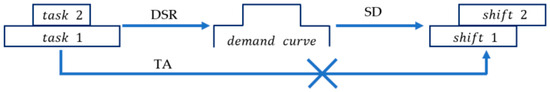
Figure 1.
The simple workforce planning processes.
If the manager uses these two shifts when making task assignments, what is likely to happen is that the employee assigned to shift 1 is made to perform task 1 by working overtime. Obviously, via such operations, not only the actual labor costs will be increased (overtime usually requires triple the hourly wage), but also a great disruption will be caused to employees’ personal lives, and the job weariness of employees will be strengthened [13]. Meanwhile, employees’ well-being will be significantly reduced under such a constantly changing schedule [14], easily leading to resignation.
To avoid this phenomenon, for task-based demand, it seems to be a good option to consider shift design and task assignment in an integrated manner. For example, multiple task sequences (each task sequence can be carried out by one person) are first generated for each alternative shift type. Then, a set cover model is used to select the appropriate shifts (task sequences). Indeed, this was a common practice in early studies of shift design with task-based demand [15].
However, the limitation of this approach lies in the fact that generating task sequences is an NP-hard problem, and enumerating all possible task sequences based on optional shift types as input to the set cover model is even more of an impossibility. Therefore, the performance of the shift plan designed via this approach depends on the sequences of tasks fed to the set cover model.
There is another common approach for shift design with task-based demand: Firstly, generating sets of tasks that can be performed by each alternative shift type and allocating sufficient workforce to each alternative shift, then considering each workforce as a different shift. Finally, using a set cover model to select the appropriate shifts/employees to minimize the number of shifts/employees used. The second method is the one that has been studied most frequently, and it was first proposed to solve the Shift Minimization Personnel Task Scheduling Problem (SMPTSP). Krishnamoorthy et al. [16] first defined SMPTP and discussed its properties, which was a variant of the Personnel Task Scheduling Problem (PTSP) but with the objective of minimizing the number of shifts/persons required to perform all tasks, and described the basic model of the problem as well as developed a heuristic algorithm that could find feasible solutions in the face of large-scale problems.
Most of the subsequent research is centered on the algorithm for solving this problem, such as Lin and Ying [17] proposed a three-stage heuristic algorithm for the SMPTSP, where a constructive heuristic algorithm was used in the first stage to quickly obtain the initial solution of the problem, an iterative greedy algorithm was used in the second stage to improve the initial solution and obtain the near-optimal solution, and finally the near-optimal solution was used as the initial solution, and used the commercial solver to further find the optimal solution. Chandrasekharan et al. [18] developed a time-based constructive matheuristic (CMH): a decomposition-based method where sub-problems are solved to optimality using exact techniques, and the optimal solutions of sub-problems are subsequently utilized to construct a feasible solution for the entire problem, which firstly solved all the difficult instances introduced by Smet et al. [19] to optimality. The current input of this method generally involves the problem of finding the maximum group of mutually exclusive tasks, which is also an NP-hard problem, so it is generally difficult to consider too many shift types and tasks. Furthermore, determining the initial number of workers for each shift type is also a problem. Too many initial configurations will lead to a sharp increase in the difficulty of solving the model, while too few will lead to no feasible solution for the model. In addition, most of the researchers of this method work on the algorithm based on a given public test set (given the optional shifts/workers and the corresponding set of performable tasks directly, with the shift type generation process hidden) without discussing the nature of the problem in more depth.
Both of the above two shift design methods with task-based demand have completed the assignment of tasks while carrying out the shift design, which has introduced other NP-hard problems and increased the difficulty of solving the problem. We believe that even in the face of task-based demand, we should return to the original intention of shift design, i.e., focus on the configuration of labor resources, while the assignment of tasks is non-essential. In this paper, we propose a new shift design model with task-based demand, which focuses more on the configuration of the workforce than the matching of workforce and demands/tasks.
Further, since, in reality, the start time of a task often deviates from the planned time, i.e., the start time of tasks is with a certain degree of randomness, if only the planned start time of a task is used for shift design, once a task arrives early or late, many tasks cannot be executed in time on the operation day, thus leading to a series of unpredictable consequences. We are therefore convinced that the uncertainty in the start time of tasks must be considered when modeling shift design with task-based demand to make the designed shift plan robust. Such a robust shift plan can guarantee that the corresponding cost of overstaffing and understaffing will not change significantly when the staffing requirements estimated are deviated [20].
However, there is a paucity of literature on the problem of shift design with stochastic demand and even less on the stochastic problem of shift design with task-based demand.
Elahipanah et al. [21] considered the shift design and task assignment problem with uncertain demand by adjusting the original shifts, reassigning tasks, and scheduling temporary shifts before the operating day to meet the demand where the randomness has become sufficiently small. However, this approach relies on the availability of temporary workers and requires that the uncertainty in demand be reduced sufficiently before the operating date. Zhen [22] used a multi-scenario approach to solve this stochastic problem to minimize the expected cost when studying the task assignment problem with an uncertain workload. Maenhout and Vanhoucke [23] proposed a model for repairing shift schedules with minimum variation after tasks are perturbed and used a meta-heuristic algorithm to solve the model, which has constraints similar to those of the SMPTSP except that the objective is to minimize perturbations, unlike expressing the staffing to perform tasks in terms of costs for over- and understaffing. Hur et al. [24] studied the stochastic problem of shift design by using the sample average approximation method to convert the stochastic model into a MILP model, then solving this model via the Lagrangian decomposition method and the subgradient method. Bürgy et al. [25], in their study of the employee scheduling problem in retail stores, considered temporary demand perturbations, developed two robust models of employee scheduling, and used multiple scenarios to simulate real-life situations. Poullet and Parmentier [26] introduce a shift design problem considering delay costs in the context of flight delays. The model takes alternative shifts containing task sequences as input data, and uses methods such as column generation to quickly obtain a shift solution with lower expected costs by continuously optimizing the set of alternative shifts and testing the delay costs of the solution under different delay scenarios. Liu et al. [27] considered the uncertainty of aircraft departure time when studying the task assignment problem at airport check-in counters, described the stochastic problem by building a multi-scenario model, and introduced the objectives and constraints of the risk aversion model, and then solved the problem using the sample average approximation and the progressive hedging algorithm, respectively.
From the relevant scientific literature on shift design and task assignment with uncertainty in demand/tasks, there are two main approaches to solving such stochastic problems: one is to wait for the randomness of demand/tasks to reduce to a low enough level to go for rescheduling, while another is to simulate the stochastic demand/tasks of the real environment via multiple scenarios of demand/tasks and find a robust solution based on those scenarios. The former approach requires the demand/task uncertainty to be reduced sufficiently small before the operational day to ensure the rescheduled solution is feasible. The latter approach usually expresses the degree of over- and understaffing in terms of expected cost. However, evaluating the reliability of a solution solely in terms of expected cost is also problematic. This is because what we can know is just the expected cost of the shift plan designed if it is applied in real environments, but not the probability that understaffing will occur. Only when the level of the demand/task’s stochasticity is reduced low enough can the dispatchers know what measures to take to cope with the coming demand/tasks, making it difficult to use such a robust shift plan? Therefore, a probability constraint on describing the probability that all tasks in the task set can be performed when using the designed shift plan should be added when constructing the stochastic model of shift design with task-based demand.
The contributions of this paper are to propose a shift design model with task-based demand, give a stochastic version of this model with a probability constraint, and develop two heuristics for solving this stochastic model. Besides, the effectiveness of these methods is demonstrated in numerical experiments.
The rest of the paper is organized as follows: Section 2 describes the deterministic shift design model with task-based demand and the corresponding stochastic version. Section 3 proposes two scenario-based heuristics for solving the stochastic model. We evaluate the performances of these proposed heuristics via numerical experiments in Section 4, and conclusions are given in Section 5.
2. Problem Description
The shift design problem for task-based demand can be stated as follows:
For a given set of tasks and a set of alternative shifts , the decision maker needs to select the appropriate shift types from and allocate the appropriate manpower to each selected shift type so that all the tasks in can be assigned sufficient manpower so that the individual tasks can be performed successfully. And each shift in the set of shifts has the parameters , refers to the start time of the shift , refers to the end time of the shift , and refers to the workforce configured for the shift . Note that is the decision variable in the shift design model and is replaced by . Similarly, each task in has parameters , where refers to the start time of task , refers to the end time of task , and refers to the workforce required to perform task k.
The following constraints are followed when designing a shift plan:
- All tasks are uninterruptible;
- manpower can be transferred from a shift to perform a task only if the start time as well as the end time of the task fall within this shift’s working duration;
- A single manpower can only perform a single task at the same time;
- manpower to perform a task can come from more than one shift.
In solving this problem, the optimization direction is to minimize the cost of the designed shift plan. For instance, as shown in Figure 2, suppose that we have designed shift 1 based on task 1 and task 2, where , , and are the start time of task 1, task 2, and shift 1, respectively; , , and are the end times of task 1, task 2, and shift 1, respectively; and are the required workforce for task 1 and task 2, respectively, and is the staffing allocated for shift 1, where . Then we call the overstaffing and the understaffing. Both overstaffing and understaffing are part of the objective function regarding the cost of the shift design model. It is important to note that the cost of understaffing referred to here does not mean that tasks can be performed without enough workforce required, but rather that dispatchers need to ensure the successful execution of tasks by outsourcing tasks, delaying the departure time of employees on duty or urgently calling back employees who are on leave.
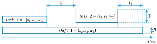
Figure 2.
The cost components of the shift design with task-based demand.
Since the model proposed in this paper is based on the traditional shift design model 12, i.e., we need to discretize the workforce required for a single task into the workforce required for each of its work periods. The work periods of a single task are determined, as shown in Figure 3. Suppose the start and end times of task k are located at the time slot and , respectively, then we consider time slots to as work periods of task k. The more periods the planning period is discretized into (the shorter the duration of each period), the more accurate this description will be, but at the same time, it will also make the model more difficult to solve.
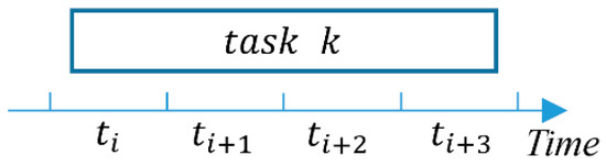
Figure 3.
The work periods of task .
Unlike the traditional shift design model, the model proposed in this paper considers the correlation between the staffing requirements at successive periods, i.e., the tasks from which the staffing requirements at each period originate. The model can be described as model M1 in Appendix A.
Further, for deterministic problems, the start time, and the end time of the task are fixed, i.e., and are constants. However, in reality, the start time and the end time of the task are often random, which means that and are actually random 0–1 variables. To facilitate the distinction between deterministic and stochastic models, we re-represent them in the stochastic version with and , respectively. Thus, we can rewrite the deterministic model above as the stochastic model M2 in Appendix B.
In addition, taking into account the growing demand for the competence of employees in various industries and the danger and confidentiality of some jobs, simply outsourcing work or temporarily notifying those employees who are on leave to come back to work [13] or force those who are on-duty to work overtime [28,29] is no longer feasible to satisfy the understaffing demand. Therefore, we introduce a probability constraint to describe the probability that all tasks in the task set can be performed using the designed shift plan in model M2 in Appendix B.
3. Solution Approach
This section will propose two stochastic methods for solving the stochastic problem mentioned in the previous section. One is a simple one-stage heuristic (OSH): First, obtain the probability of each task occupying every time slot as a work period through a large number of randomly generated scenarios so that a shift plan that both satisfies the probability constraint (A9) and performs well in terms of cost can be found by relaxing the range of work slots for the tasks. The other is a two-stage heuristic (TSH): In the first stage, obtain a series of shift plans by continuously generating scenarios to evaluate the performance of the shift plan designed/revised and thus continuously revising the shift plan designed/revised. In the second stage, use a search algorithm to find a shift plan in the shift plan set obtained in the first phase that both satisfies the probability constraint (A9) and performs well in terms of cost. Both of these approaches involve a shift design model without over- and understaffing cost, which we call M3, and a task assignment algorithm (TAA) whose core idea is to evaluate the expected performance of the shift plan by using a greedy strategy to simulate a realistic dispatchers’ assignment of tasks during the operational day.
In the following, we will give the specific formulation of the model M3 in Section 3.1, then describe the task assignment algorithm we use in Section 3.2, followed by Section 3.3 and Section 3.4 to show the two heuristics we propose, respectively.
3.1. Shift Design Model M3
The model M3 is described in Appendix C.
3.2. Task Assignment Algorithm
Before describing the TAA, we state the following definition:
For a given designed shift plan , denote the i-th shift in by , and the corresponding shift has the following information , where and are the start time and end time of shift , respectively, and is the staffing for shift . The inherent cost of shift plan is .
Also for any shift , there are subshifts, and each subshift has the following information . The subshifts of each shift are collected to generate a new set of subshifts , and the i-th shift in is denoted by .
And for a given set of tasks , is the j-th task in with the following information , where and are the start time and end time of task , respectively, and is the workforce required to perform task .
To some extent, each shift can also be viewed as a task, and we will use this feature in the first phase of the TSH.
The specific process of TAA is as follows:
- Step 1
- For a given designed shift plan , generate the corresponding set of subshifts and make the tasks in sorted by the start time of the tasks. Initialize , create an empty set , and go to step 2.
- Step 2
- If , then let , collect the subshifts that can dispatch workforce to the j-th task from the set to generate a new set , where , and sort the shifts in from front to back according to the start time of shifts. Use to denote the i-th shift in , update with =, and go to Step 3; otherwise go to Step 4.
- Step 3
- Compute , , where if , then , , and let ; otherwise ,, and let , and then generate a new task with the information , add task to , update , =, and go to Step 2.
- Step 4
- Compute , where and output and .
is the over- and understaffing cost of the shift plan when this plan is used in the scenario , and is the corresponding set of those tasks without workforce to perform.
3.3. One-Stage Heuristic
As shown in Figure 4, if the start time of task obeys the probability density function , then we can randomly generate a large number of scenarios based on this function (task a, b, and c are one possible scenario for task , respectively). Based on these scenarios, we can count the probability that time slot t is a work period for task . Thus we can introduce the following equation.
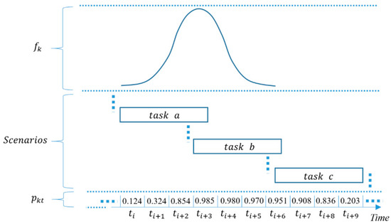
Figure 4.
The work periods with a probability of task k.
Formula (1) indicates that when the probability that time slot is a work period for task is not less than ( takes values in the range of ), then time slot is considered a working slot for task . The closer the value of is to 0, the more working slots task k has, and if the workforce is allocated to task k according to these slots via the shift design model, the higher is the probability that task can be allocated sufficient workforce on the operation day.
The one-stage heuristic proposed below is to adjust the value of to obtain a shift plan that satisfies the probability constraint (A9) and performs well in terms of cost.
The specific algorithm is as follows:
- Step 1
- Count via for . Initialize the parameters , and go to step 2.
- Step 2
- Update via constraint (1) and find the corresponding optimal shift plan via M3. Generate M scenarios by perturbing the start time of tasks in task set K. Take and each of these M scenarios as the input of TAA, respectively, and denote the number of occurrences by . Let , and calculate the inherent cost and the expected cost of the shift plan , where , . If , then go to Step 3; otherwise go to Step 6.
- Step 3
- Let . If , then go to Step 6, otherwise go to Step 4.
- Step 4
- Update via constraint (1) and update the shift plan via M3, respectively. Generate M scenarios by perturbing the start time of tasks in task set . Take and each of these M scenarios as the input of TAA, respectively, denote the number of occurrences by , and let . If , then go to Step 5; otherwise let and go to Step 3.
- Step 5
- If , then let and go to Step 3; otherwise, let and go to Step 3.
- Step 6
- Output and .
is a shift plan that satisfies the probability constraint (A9) while performs well in terms of the expected cost (the expected cost of this plan is ), and the probability that this shift plan can provide a sufficient workforce for all tasks in K on the operation day via TAA is .
3.4. Two-Stage Heuristic
In this subsection, we propose a scenario-based two-stage heuristic algorithm (TSH) to solve the previously mentioned stochastic problem. In the first phase, we will propose an algorithm to modify the shift plan designed and generate the set of modified shift plans. The algorithm process is roughly as follows. First, generate an initial shift plan via M3, and then generate a possible scenario by perturbing the start time of each task in the original set of tasks. Suppose the initial shift plan cannot provide sufficient workforce for all tasks in this scenario. In that case, the tasks with insufficient workforce and the initial shift plan are considered as a new set of tasks, and this new set of tasks is used as input to M3 to find a new shift plan (this new shift plan is called the revised shift plan). Then generate a new scenario again, and if the revised shift plan still cannot provide all tasks with a sufficient workforce, revise the shift plan again and repeat the process until there is a revised shift plan that continuously passes the test for a certain number of scenarios (the revised shift plan can provide enough labor for all tasks in any one of these scenarios). Record each revised shift plan in the process to generate a revised shift plan set and terminate the first stage of the algorithm. In the second phase, we will develop a search algorithm. This bisection method combines the Monte Carlo method for searching the revised shift plan set generated in the first phase for a shift plan that meets the probability constraint (A9) and performs relatively well in cost.
3.4.1. The First Phase of TSH
The specific algorithm is as follows:
- Step 1
- Initialize parameters, let , , and go to step 2.
- Step 2
- For the given alternative shift set and the task set , find an initial shift paln via the model M3, and let = , then go to step 3.
- Step 3
- Obtain the new scenario by perturbing the start time of the tasks in (assuming that the execution time of each task is constant), use and as the input of TAA to obtain the corresponding output , and go to step 4.
- Step 4
- If , let and go to step 5; otherwise let and go to step 6.
- Step 5
- Treat the shifts in as tasks and generate a new task set , where . Use and as inputs for M3 to find the corresponding shift plan and let , = , then go to step 3.
- Step 6
- If , then go to step 3; otherwise go to step 7.
- Step 7
- Generate a revised shift plan set , where , and output .
is the collection of all shift plans generated in the first phase, and it is also the input for the second phase.
3.4.2. The Second Phase of TSH
Use to denote the d-th shift plan in the set . Since in the set derived in the first stage, the later the shift plan is designed, the more scenarios can be covered, i.e., the coverage of each shift plan in increases as d increases. Therefore, we can use the bisection method to search for a shift plan from that both satisfy the probability constraint (A9) and perform well in terms of cost.
The specific algorithm is as follows:
- Step 1
- Initialize the parameters . Use to denote the d-th shift plan in the shift plan set and go to step 2.
- Step 2
- Generate M scenarios by perturbing the start time of tasks in task set K. Take and each of these M scenarios as the input of TAA, respectively, and denote the number of occurrences by . Let ,,, and calculate the inherent cost and the expected cost of the shift plan , where , . If , then go to Step 3; otherwise go to Step 6.
- Step 3
- Let . If , then go to Step 6, otherwise go to Step 4
- Step 4
- Generate M scenarios by perturbing the start time of tasks in task set K. Take and each of these M scenarios as the input of TAA, respectively, denote the number of occurrences by , and let . If , then go to Step 5; otherwise, let and go to Step 3.
- Step 5
- If , then let and go to Step 3; otherwise, let and go to Step 3.
- Step 6
- Output and .
is a shift plan that satisfies the probability constraint (A9) while performs well in terms of the expected cost (the expected cost of this plan is ), and the probability that this shift plan can provide a sufficient workforce for all tasks in K on the operation day via TAA is .
4. Numerical Results
This section first shows the impact of the relevant parameters on both methods proposed in this paper. Further, it compares the performance of these two algorithms under their respective superior parameters. All calculations are performed on a computer with an AMD R5 4600H Radeon Graphics @ 3.0 GHz, 16 G of RAM. And the commercial solver to solve model M3 is Gurobi 9.0.1.
In subsequent experiments, we consider only one planning day, which starts at 4:00 a.m. on a normal calendar day and ends after 24 h. In addition, we split the planning day into 288 equal-size time slots , the lengths of which are h, and indicates the start time of the planning day. Denote the time slot set and the time point set.
Due to not considering the shift breaks, we can describe the alternative shift set as , where denotes shift start time, denotes shift end time, means that the alternative shift lengths are 6 to 10 h, and indicates that all shifts can only start or end every half hour.
The original data we use in the following experiments are originated from a Chinese mega-airport operational department, and the probability density function obeyed by the start time of all tasks is estimated via statistical methods (there is a lack of sufficient data to estimate the probability density function of the start time of each task ). Therefore, the scenarios used to test the solutions found by OSH and TSH are generated based on the original task set and function .
4.1. The Effect of the Scale of Ω on the Performances of OSH
In this subsection, we test the effect of different sizes of scenario set Ω on the performances of OSH. Fix the parameters , and vary the size of with . Carry out 20 times each experiment and calculate the average of these experiments result. In addition, regenerate the scenario set before starting each experiment.
Figure 5 shows that as the scale of the scenario set Ω increases, the maximum expected task coverage of the shift plan found via OSH will gradually approach 1, while the expected cost and solution time of the corresponding shift plan will also increase. When the number of scenarios increases to a certain level, the maximum expected task coverage, cost and runtime of OSH will stabilize (the maximum expected coverage is slightly less than 1), i.e., increasing the scale of scenarios again will not cause significant changes in the maximum expected coverage, cost and runtime. Among them, the reason that the expected cost and the expected task coverage of OSH first increase and then stabilize with the increasing scenario scale is that only when the number of scenarios is large enough, the real situation be better simulated, or it is more likely to find out the potential work periods of each task. In addition, the number of non-zero terms in model M3 increases as more potential work periods for each task are explored, and the number of non-zero terms in model M3 stabilizes when the number of scenarios used is sufficiently large, which is why the expected solution time of OSH also increases and then stabilizes with the increasing scenario scale.
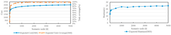
Figure 5.
The impact of the scenario number on the performances of OSH.
4.2. The Effect of the Accuracy of Value on the Performances of OSH
The effect of the accuracy of value ϵ on the performance of OSH is tested in this subsection. Fix the parameters α = 1, γ = 0.5, δ = 3, M = 8000, |Ω| = 5000, η = 0.95 and vary the accuracy of ϵ with ϵ = 0.01, 0.001, 0.0001, 0.00001, 0.000001, 0.0000001. Carry out 20 times each experiment and calculate the average of these experiments result. In addition, regenerate the scenario set before starting each experiment.
Figure 6 shows that the expected cost and expected coverage of OSH first decrease and then stabilize as the accuracy of the value ϵ is increased. This is because when the accuracy of value ϵ is increased, OSH can find better solutions near the feasible solution, and when OSH has found a locally optimal solution near the feasible solution, at this point, increasing the accuracy of value ϵ again will not have an optimizing effect on the solution. In addition, the running time of OSH increases significantly (exponentially) with the increase in the precision of ϵ. This is because each increase in the precision of the value ϵ by an order of magnitude doubles the number of searches of the dichotomy in OSH.
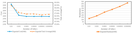
Figure 6.
The impact of the accuracy of value ϵ on the performances of OSH.
4.3. The Effect of the Value N on the Performances of TSH
The effect of the value N taken on the performance of TSH is tested in this subsection. Fix the parameters α = 1, γ = 0.5, δ = 3, M = 8000, η = 1 and vary the value of N with . Carry out 20 times each experiment and calculate the average of these experiments result.
Similar to Figure 5, Figure 7 shows that as scenario number N increases, the maximum expected task coverage of the shift plans found by TSH will gradually approach 1, while at the same time, the expected cost of the corresponding shift plans will increase. This is due to the fact that when increasing the scenario number, TSH will discover a bad scenario to which the current shift plan found is not applicable, for which TSH will update the shift plan to improve the robustness of the shift plan, but at the same time, it also increases the cost of the shift plan. When the scenario number increases to a certain level, the maximum expected coverage and the expected cost of the shift plans found by TSH will stabilize (the maximum expected coverage is slightly less than 1) because the number of scenarios the shift plan can cope with is sufficiently large. It is very difficult to appear in bad scenarios that cannot be coped with by the shift plan anymore. In addition, the runtime of TSH increases (linearly) with N. This is because increasing scenario number N corresponds to increasing test times for the shift plan in TSH.
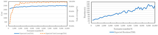
Figure 7.
The impact of the value N taken on the performances of TSH.
4.4. The Effect of the Scenario Scale M on the Expected Performance Stability of the Shift Plan
The effect of the number of scenarios used to calculate the expected performance metrics for the shift plans on the stability of the metrics is tested in this subsection. Randomly select 20 shift plans in the previous section to generate a set , and use to denote the d-th shift plan in the set. Vary the value of with , and use to denote the i-th value of where has values. Fix the parameters . For each plan and each value of , we can generate scenarios and use TAA to calculate the corresponding expected cost and expected coverage .
Then denote the stability of the expected cost and expected coverage of the shift plan with by and , respectively. The formulas of and are as follows:
Figure 8 indicates that as the number of scenarios used to calculate the shift plan increases for the metrics, the expected cost of the shift plan will fluctuate less with the expected coverage, i.e., the expected performance calculated for each shift plan will be accurate only if the number of scenarios is sufficient. This result follows the law of large numbers.
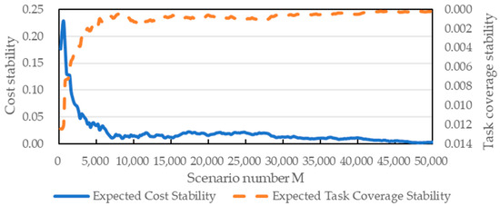
Figure 8.
The impact of scenario number M on the stability of the expected metrics of shift plan.
4.5. The Effect of the Task Coverage η on the Performances of OSH and TSH
The effect of the task coverage η on the performances of OSH and TSH is tested in this subsection. Fix the parameters and vary the value of with . Carry out 20 times each experiment and calculate the average of these experiments result. In addition, regenerate the scenario set before starting each experiment.
Figure 9 shows that as the task coverage η increases, the expected cost of the solutions found by both methods under their respective better parameters increases, which is the cost of additional resources to overcome the bad scenario. And when requiring a task coverage η of 1, the expected cost of shift plans found by both methods increases dramatically, due to the diminishing marginal benefit effect. Among them, the solutions found by TSH are always cost-advantageous, and the advantage is more pronounced the higher the task coverage η is. This is because OSH finds the feasible solution by relaxing the resource occupancy time of all tasks simultaneously, while TSH updates the feasible solution by iterating, which makes the cost of the shift plan found by TSH lower than that of OSH.
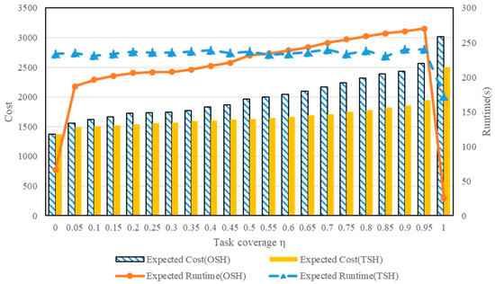
Figure 9.
The impact of the task coverage η on the performances of OSH and TSH.
In addition, the running time of OSH increases with the task coverage η, while the running time of TSH remains relatively stable. This is because increasing the task coverage η increases the non-zero term in the M3 model used by OSH, which increases the running time of OSH, whereas TSH always first finds a shift plan with task coverage close to 1 before using dichotomization to find a shift plan that satisfies the task coverage η and performs well in terms of cost in the updating process. Besides, when the required task coverage η is 1, the running time of both methods drops dramatically. This is because the task coverage of the solutions found by both methods can only be close to 1. Both methods use backtracking to find a solution that satisfies the constraint (A9), so both algorithms terminate as soon as the initial backtracked solution does not satisfy the constraint (A9), which is why the running time is so short at this time.
5. Conclusions
In this paper, an original model is proposed for the shift design problem with task-based demand, and a stochastic version is given, to which a probability constraint is added according to practical needs to describe the probability that the workforce allocated by the shift plan designed can satisfy the workforce required by all tasks.
In addition, this paper proposes two methods (OSH and TSH) to solve this stochastic model. OSH is a one-stage heuristic that is commonly used in factories to enhance the robustness of routing. In this paper, we enhance the robustness of the shift plan by increasing the resource occupancy time for each task. The advantage of this method is that the method is simple and easy to implement, but the disadvantage is that the resource occupancy time of all tasks is increased synchronously, which leads to the high cost of the solution. Therefore, we propose a two-stage heuristic (TSH) that combines the optimization model with a simulation method. Firstly, we find an initial shift plan and test the feasibility of the plan by a simulation method. Then, we correct the inputs of the optimization model based on the test results. And iterate the process multiple times to obtain a feasible solution that satisfies the probabilistic constraints (A9). The advantage of this method is that each iteration of the optimization is searching for the solution with the optimal cost, thus slowing down the increase in the cost of the shift plan.
Further, the experimental results show that: (1) Only when the scale of scenarios used to simulate the real situation are large enough the reliability of the solution can be high enough; (2) Only when the scale of the scenarios used to calculate the expected performance of the solution reaches a certain level, the calculated performance indexes can be sufficiently accurate and stable; (3) Under relatively better parameter settings in each of the two solution methods, TSH always outperforms OSH in terms of the cost of the solution, and the running time of TSH is more stable; (4) There is a law of diminishing marginal benefit for the robustness solutions found by both methods, i.e., each enhancement in the robustness of the solution requires more additional cost, and the cost of the solution increases dramatically when the risk of pursuing the solution approaches zero.
In summary, we recommend that managers use TSH to find robust shift plans and use as many scenarios as possible when finding solutions and calculating the expected metrics. Finally, managers should also be aware that pursuing a solution with an understaffing risk close to zero will significantly increase the cost of the solution.
The stochastic problem considered in this paper (the randomness of the task cannot be reduced low enough before the operation date) has no way to find the optimal solution to compare the degree of merit of the solutions found by each method for the time being. The solution derived from the OSH proposed in this paper can be considered a benchmark. In addition, if the randomness of tasks can be reduced sufficiently before the operating day, the TAA proposed in this paper can be replaced by a conventional task assignment model, or even the stochastic model proposed in this paper can be directly converted into a conventional deterministic integer programming model via the sample average approximation method [30], and the corresponding optimal solution can be found by using commercial solvers (the sample size of the model for approximating the realistic situation may be relatively so large that the solution time of the model is unacceptable).
Furthermore, the TSH proposed in this paper lacks a supervisory means to avoid the designed or modified shifts from encountering the worst-case scenario prematurely in the first stage, which has a certain probability of causing the cost of shifts to rise too fast. Therefore, in future research, it is worthwhile to investigate the development of new methods to find the optimal solution to the stochastic problem considered in this paper and the inclusion of controls in TSH to avoid excessive increases in shift costs.
Author Contributions
Conceptualization, Z.W. and Q.C.; Methodology, Z.W. and Q.C.; Software, Z.W.; Validation, G.X.; Formal analysis, G.X.; Writing—original draft, Z.W.; Visualization, G.X.; Supervision, N.M.; Project administration, N.M. All authors have read and agreed to the published version of the manuscript.
Funding
This research was supported by the National Natural Science Foundation of China (No.61973089).
Data Availability Statement
The data are not publicly available due to restrictions e.g., privacy or ethical.
Conflicts of Interest
The authors declare no conflict of interest.
Abbreviations
| set of time periods within the planning horizon; | |
| set of alternative shifts; | |
| set of tasks; | |
| cost per staff per hour | |
| cost per overstaff per hour | |
| cost per understaff per hour | |
| the probability that all tasks have a sufficient workforce to be carried out | |
| the length of shift | |
| the length of task | |
| the length of a single time slot | |
| staffing requirements of task k | |
| binary parameter that takes the value 1 if time slot is a work period for shift , 0 otherwise | |
| binary parameter that takes the value 1 if time slot is a work period for task , 0 otherwise | |
| random binary parameter that takes the value 1 if time slot is a work period for task , 0 otherwise | |
| binary parameter that takes the value 1 if the work periods of shift can cover the work periods of task , 0 otherwise | |
| random binary parameter that takes the value 1 if the work periods of shift can cover the work periods of task , 0 otherwise | |
| overstaffing for shift in time slot , | |
| understaffing for task , | |
| staffing for shift , ; is a -dimensional vector consisting of | |
| workforce assigned to task k from shift h, | |
| cost of overstaffing in assigning workforce to the j-th task | |
| cost of understaffing in assigning workforce to the j-th task | |
| additional cost of shift plan , consisting of over- and understaffing cost | |
| set of tasks without workforce to perform | |
| set of scenarios generated to approximate the stochastic problem; | |
| a threshold value used to terminate the algorithm | |
| a sufficiently small constant; | |
| M | number of scenarios used to obtain the expected cost of the shift plan |
| N | The number of scenarios for which the revised shift plan needs to pass the test consecutively when terminating the algorithm. |
Appendix A
M1
Subject to
Objective (A1) is to minimize the cost, which comprises the inherent cost of every shift itself, the cost of understaffing for every task, and the cost of overstaffing for every shift in every time slot. Constraint (A2) ensures that the sum of the workforce dispatched to task from each shift plus the understaffing for task is equal to the staffing requirements of task . Constraint (A3) ensures that the staffing for shift minus the overstaffing of shift during time slot is equal to the sum of the workforce dispatched to every task from shift during time slot . Constraint (A4) states the integrality conditions on variables.
Appendix B
M2
Subject to
The objective function (A5) minimizes the cost function, which is an expectation function on staffing, over- and understaffing. Constraints (A6)–(A8) have similar meanings as constraints (A2)–(A4).
The symbol referred to as task coverage, indicates the probability that all tasks can be performed with sufficient staff. And the probability constraint ensures that the probability that all tasks can be performed with sufficient staff is not less than the value .
Appendix C
M3
Subject to
The objective function minimizes the cost, which only consists of the inherent cost of every shift. Constraint ensures that the sum of the workforce dispatched to task from each shift is equal to the staffing requirements of task . Constraint ensures that the staffing for shift during time slot is not less than the sum of the workforce dispatched to every task from shift during time slot . The domains of variables are stated in constraint .
References
- Wu, Z.; Xu, G.; Chen, Q.; Mao, N. Two stochastic optimization methods for shift design with uncertain demand. Omega 2023, 115, 102789. [Google Scholar] [CrossRef]
- Smet, P.; Lejon, A.; Berghe, G.V. Demand smoothing in shift design. Flex. Serv. Manuf. J. 2021, 33, 457–484. [Google Scholar] [CrossRef]
- Ingels, J.; Maenhout, B. Optimised buffer allocation to construct stable personnel shift rosters. Omega 2019, 82, 102–117. [Google Scholar] [CrossRef]
- Becker, T. A decomposition heuristic for rotational workforce scheduling. J. Sched. 2020, 23, 539–554. [Google Scholar] [CrossRef]
- Guo, J.; Bard, J.F. A column generation-based algorithm for midterm nurse scheduling with specialized constraints, preference considerations, and overtime. Comput. Oper. Res. 2022, 138, 105597. [Google Scholar] [CrossRef]
- Mansini, R.; Zanella, M.; Zanotti, R. Optimizing a complex multi-objective personnel scheduling problem jointly complying with requests from customers and staff. Omega 2023, 114, 102722. [Google Scholar] [CrossRef]
- Moosavi, A.; Ozturk, O.; Patrick, J. Staff scheduling for residential care under pandemic conditions: The case of COVID-19. Omega 2022, 112, 102671. [Google Scholar] [CrossRef] [PubMed]
- Wolbeck, L.; Kliewer, N.; Marques, I. Fair shift change penalization scheme for nurse rescheduling problems. Eur. J. Oper. Res. 2020, 284, 1121–1135. [Google Scholar] [CrossRef]
- Hassani, R.; Desaulniers, G.; Elhallaoui, I. Real-time bi-objective personnel re-scheduling in the retail industry. Eur. J. Oper. Res. 2021, 293, 93–108. [Google Scholar] [CrossRef]
- Wang, F.; Zhang, C.; Zhang, H.; Xu, L. Short-term physician rescheduling model with feature-driven demand for mental disorders outpatients. Omega 2021, 105, 102519. [Google Scholar] [CrossRef]
- Breugem, T.; van Rossum, B.; Dollevoet, T.; Huisman, D. A column generation approach for the integrated crew re-planning problem. Omega 2022, 107, 10255. [Google Scholar] [CrossRef]
- Dantzig, G.B. Letter to the Editor—A Comment on Edie’s “Traffic Delays at Toll Booths”. J. Oper. Res. Soc. Am. 1954, 2, 339–341. [Google Scholar] [CrossRef]
- Åkerstedt, T.; Kecklund, G. What work schedule characteristics constitute a problem to the individual? A representative study of Swedish shift workers. Appl. Ergon. 2017, 59, 320–325. [Google Scholar] [CrossRef] [PubMed]
- Zhou, Z.; Zhang, Y.; Sang, L.; Shen, J.; Lian, Y. Association between sleep disorders and shift work: A prospective cohort study in the Chinese petroleum industry. Int. J. Occup. Saf. Ergon. 2020, 28, 751–757. [Google Scholar] [CrossRef] [PubMed]
- Ernst, A.; Jiang, H.; Krishnamoorthy, M.; Sier, D. Staff scheduling and rostering: A review of applications, methods and models. Eur. J. Oper. Res. 2004, 153, 3–27. [Google Scholar] [CrossRef]
- Krishnamoorthy, M.; Ernst, A.; Baatar, D. Algorithms for large scale Shift Minimisation Personnel Task Scheduling Problems. Eur. J. Oper. Res. 2012, 219, 34–48. [Google Scholar] [CrossRef]
- Lin, S.-W.; Ying, K.-C. Minimizing shifts for personnel task scheduling problems: A three-phase algorithm. Eur. J. Oper. Res. 2014, 237, 323–334. [Google Scholar] [CrossRef]
- Chandrasekharan, R.C.; Smet, P.; Wauters, T. An automatic constructive matheuristic for the shift minimization personnel task scheduling problem. J. Heuristics 2021, 27, 205–227. [Google Scholar] [CrossRef]
- Smet, P.; Wauters, T.; Mihaylov, M.; Vanden Berghe, G. The shift minimisation personnel task scheduling problem: A new hybrid approach and computational insights. Omega 2014, 46, 64–73. [Google Scholar] [CrossRef]
- van Hulst, D.; Hertog, D.D.; Nuijten, W. Robust shift generation in workforce planning. Comput. Manag. Sci. 2017, 14, 115–134. [Google Scholar] [CrossRef]
- Elahipanah, M.; Desaulniers, G.; Lacasse-Guay, È. A two-phase mathematical-programming heuristic for flexible assignment of activities and tasks to work shifts. J. Sched. 2013, 16, 443–460. [Google Scholar] [CrossRef]
- Zhen, L. Task assignment under uncertainty: Stochastic programming and robust optimisation approaches. Int. J. Prod. Res. 2014, 53, 1487–1502. [Google Scholar] [CrossRef]
- Maenhout, B.; Vanhoucke, M. A perturbation matheuristic for the integrated personnel shift and task re-scheduling problem. Eur. J. Oper. Res. 2018, 269, 806–823. [Google Scholar] [CrossRef]
- Hur, Y.; Bard, J.F.; Frey, M.; Kiermaier, F. A stochastic optimization approach to shift scheduling with breaks adjustments. Comput. Oper. Res. 2019, 107, 127–139. [Google Scholar] [CrossRef]
- Bürgy, R.; Michon-Lacaze, H.; Desaulniers, G. Employee scheduling with short demand perturbations and extensible shifts. Omega 2019, 89, 177–192. [Google Scholar] [CrossRef]
- Poullet, J.; Parmentier, A. Shift Planning Under Delay Uncertainty at Air France: A Vehicle-Scheduling Problem with Outsourcing. Transp. Sci. 2020, 54, 956–972. [Google Scholar] [CrossRef]
- Liu, M.; Liang, B.; Zhu, M.; Chu, C. Stochastic Check-in Employee Scheduling Problem. IEEE Access 2020, 8, 80305–80317. [Google Scholar] [CrossRef]
- Voinescu, B.I. Common Sleep, Psychiatric, and Somatic Problems According to Work Schedule: An Internet Survey in an Eastern European Country. Int. J. Behav. Med. 2018, 25, 456–464. [Google Scholar] [CrossRef]
- Brauner, C.; Wöhrmann, A.M.; Frank, K.; Michel, A. Health and work-life balance across types of work schedules: A latent class analysis. Appl. Ergon. 2019, 81, 102906. [Google Scholar] [CrossRef]
- Verweij, B.; Ahmed, S.; Kleywegt, A.J.; Nemhauser, G.; Shapiro, A. The Sample Average Approximation Method Applied to Stochastic Routing Problems: A Computational Study. Comput. Optim. Appl. 2003, 24, 289–333. [Google Scholar] [CrossRef]
Disclaimer/Publisher’s Note: The statements, opinions and data contained in all publications are solely those of the individual author(s) and contributor(s) and not of MDPI and/or the editor(s). MDPI and/or the editor(s) disclaim responsibility for any injury to people or property resulting from any ideas, methods, instructions or products referred to in the content. |
© 2023 by the authors. Licensee MDPI, Basel, Switzerland. This article is an open access article distributed under the terms and conditions of the Creative Commons Attribution (CC BY) license (https://creativecommons.org/licenses/by/4.0/).