Figure 1.
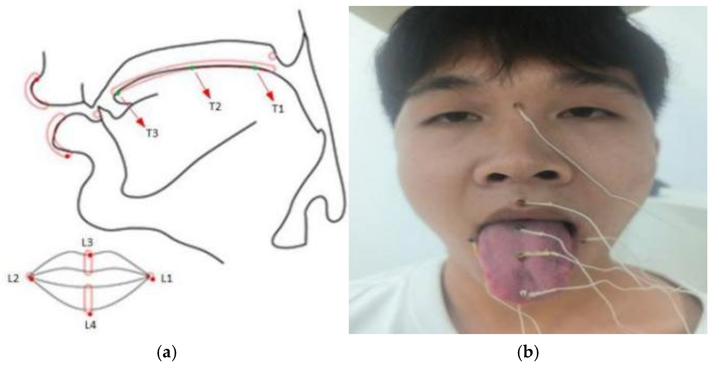
Articulatory sensor placement and participant setup for data acquisition. Participant gave permission for the use of his image. (a) Placement of EMA sensors on lips (L1–L4) and tongue (T1–T3). (b) Participant wearing EMA sensors in the recording session.
Figure 1.
Articulatory sensor placement and participant setup for data acquisition. Participant gave permission for the use of his image. (a) Placement of EMA sensors on lips (L1–L4) and tongue (T1–T3). (b) Participant wearing EMA sensors in the recording session.
Figure 2.
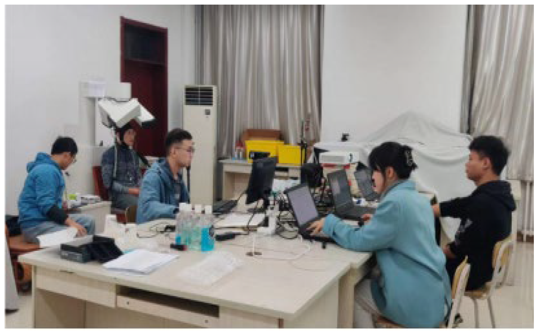
Schematic diagram of data acquisition.
Figure 2.
Schematic diagram of data acquisition.
Figure 3.
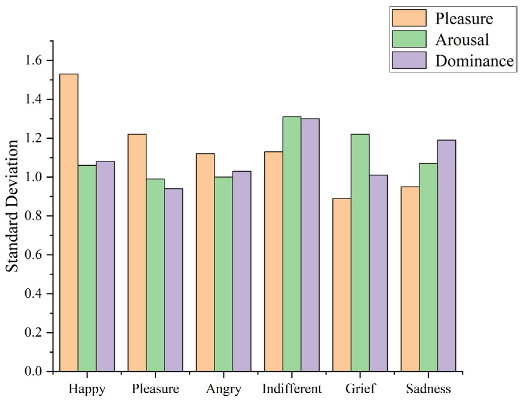
Intra-class dispersion of PAD annotations. Standard deviations of pleasure, arousal, and dominance are computed per emotion category to quantify annotation consistency across annotators.
Figure 3.
Intra-class dispersion of PAD annotations. Standard deviations of pleasure, arousal, and dominance are computed per emotion category to quantify annotation consistency across annotators.
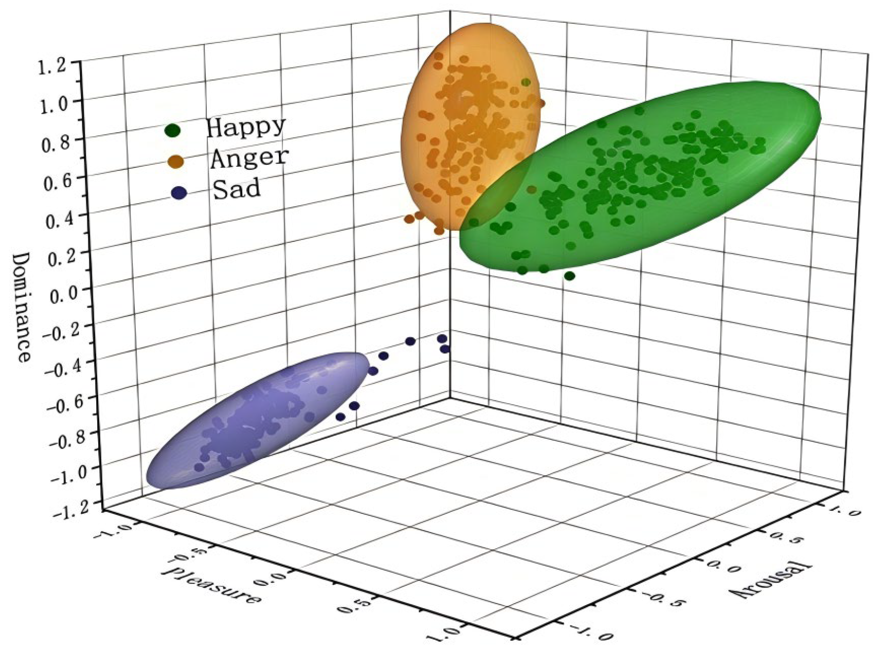
Figure 4.
PAD-space visualization of strong emotions. Each point represents the mean PAD label of a sample; ellipsoids indicate 95% confidence regions for happy, anger, and sadness, illustrating cluster separability and remaining outliers.
Figure 4.
PAD-space visualization of strong emotions. Each point represents the mean PAD label of a sample; ellipsoids indicate 95% confidence regions for happy, anger, and sadness, illustrating cluster separability and remaining outliers.
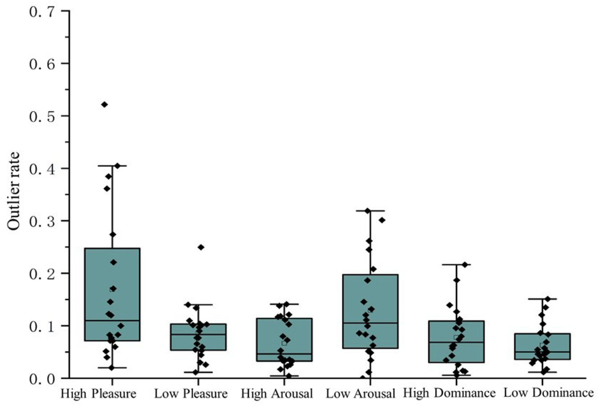
Figure 5.
Distribution of annotator outlier rates across the six high/low PAD dimension categories. The boxplots visualize the statistical dispersion of annotation error rates for the 20 annotators. Each dot represents an individual annotator.
Figure 5.
Distribution of annotator outlier rates across the six high/low PAD dimension categories. The boxplots visualize the statistical dispersion of annotation error rates for the 20 annotators. Each dot represents an individual annotator.
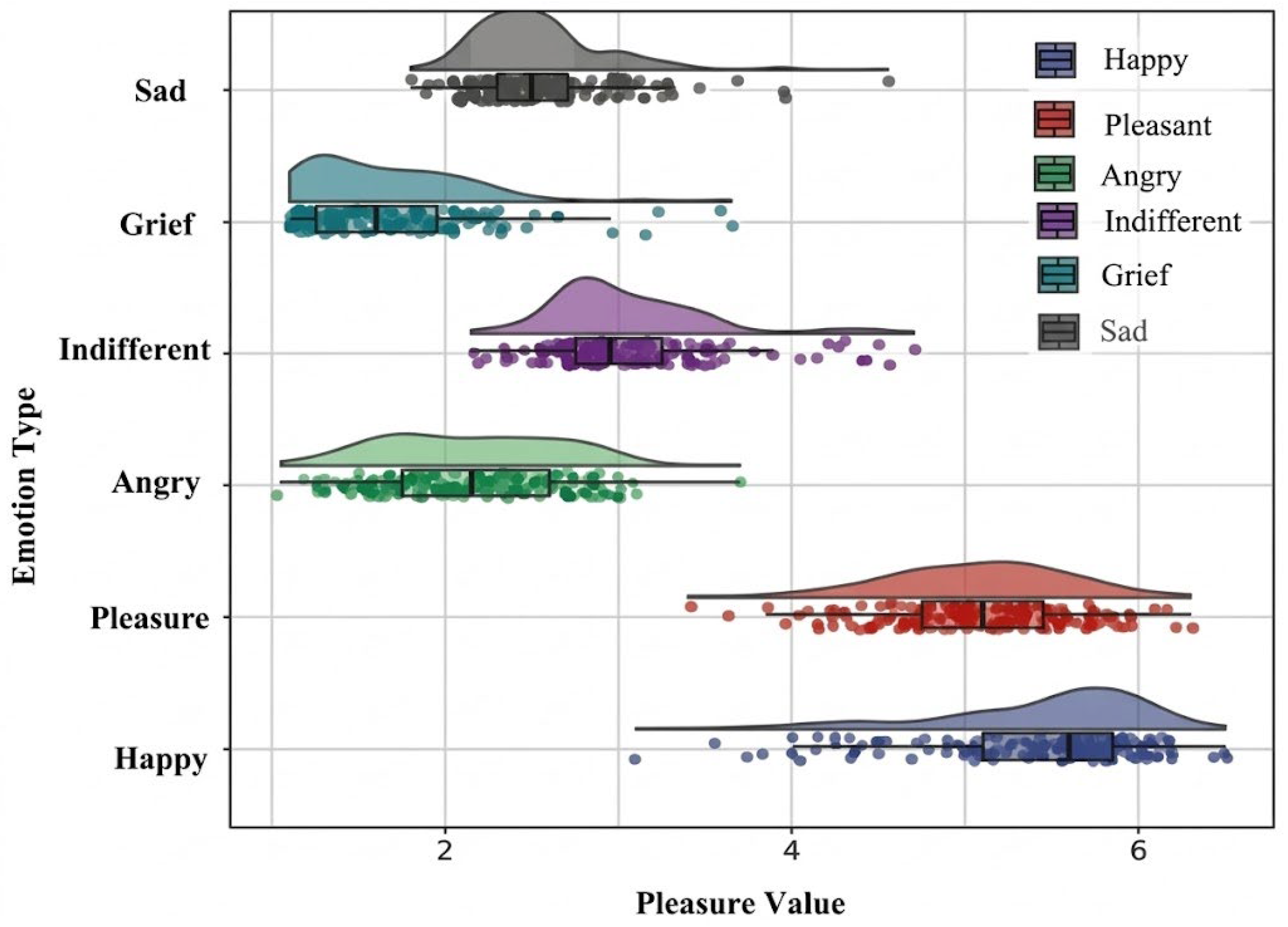
Figure 6.
The average distribution of various emotions. The “cloud and rain” graph (density estimation curve graph, box plot, and jitter scatter plot) shows the distribution of the degree of pleasure across the six emotional categories.
Figure 6.
The average distribution of various emotions. The “cloud and rain” graph (density estimation curve graph, box plot, and jitter scatter plot) shows the distribution of the degree of pleasure across the six emotional categories.
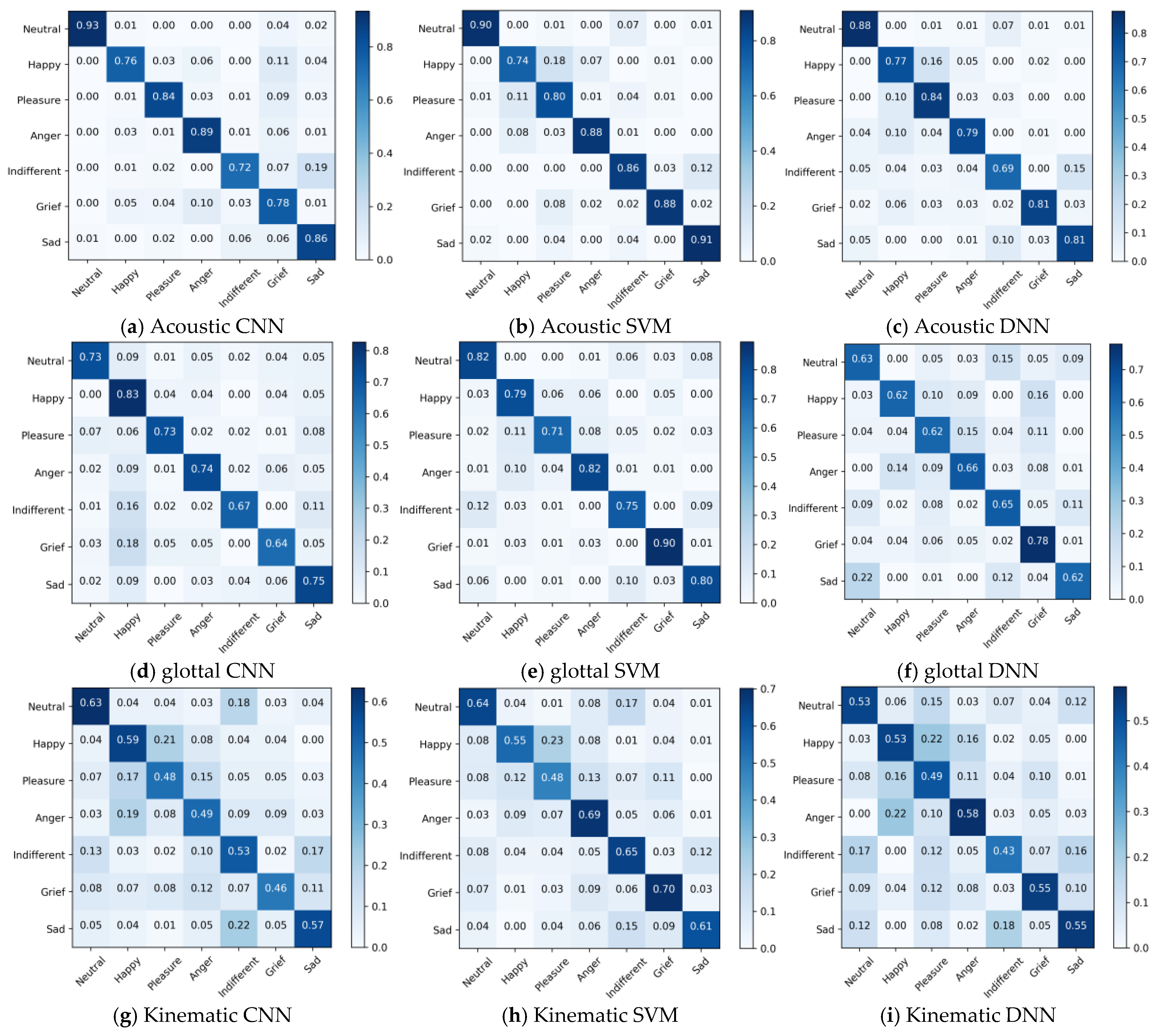
Figure 7.
Confusion matrices of unimodal baselines on STEM-E2VA. Rows denote ground-truth emotion classes and columns denote predicted classes; panels (a–i) correspond to CNN/SVM/DNN models for acoustic, glottal, and kinematic modalities.
Figure 7.
Confusion matrices of unimodal baselines on STEM-E2VA. Rows denote ground-truth emotion classes and columns denote predicted classes; panels (a–i) correspond to CNN/SVM/DNN models for acoustic, glottal, and kinematic modalities.
Figure 8.
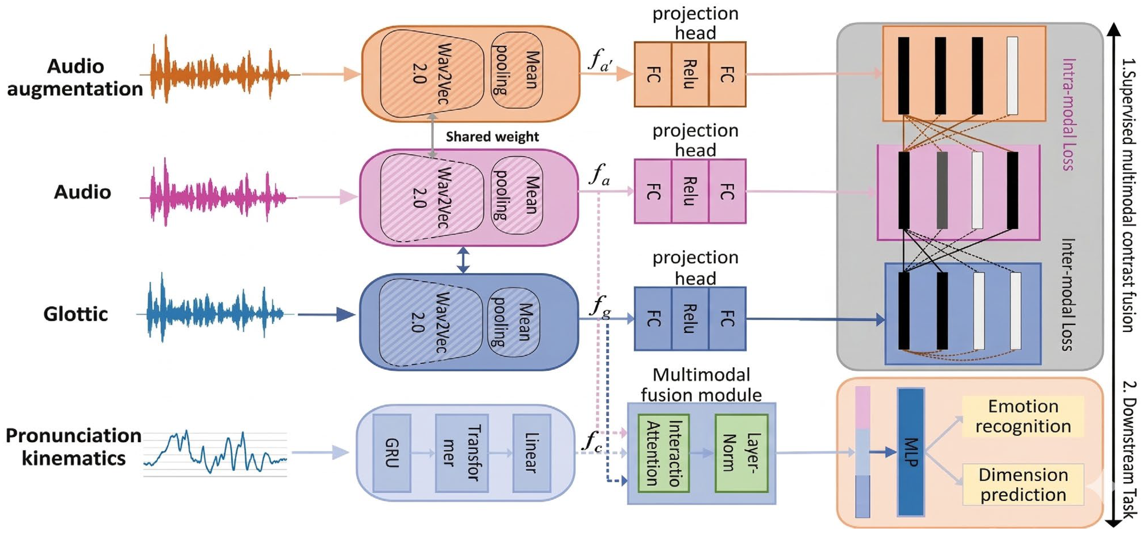
Overview of the PAD-guided multimodal hybrid contrastive framework. In this framework, Wav2Vec 2.0 encodes acoustic and glottal signals, and a GRU–Transformer models articulatory kinematics. These representations are optimized by MMCL-PAD and integrated using an interactive attention fusion module to achieve discrete classification and PAD regression.
Figure 8.
Overview of the PAD-guided multimodal hybrid contrastive framework. In this framework, Wav2Vec 2.0 encodes acoustic and glottal signals, and a GRU–Transformer models articulatory kinematics. These representations are optimized by MMCL-PAD and integrated using an interactive attention fusion module to achieve discrete classification and PAD regression.
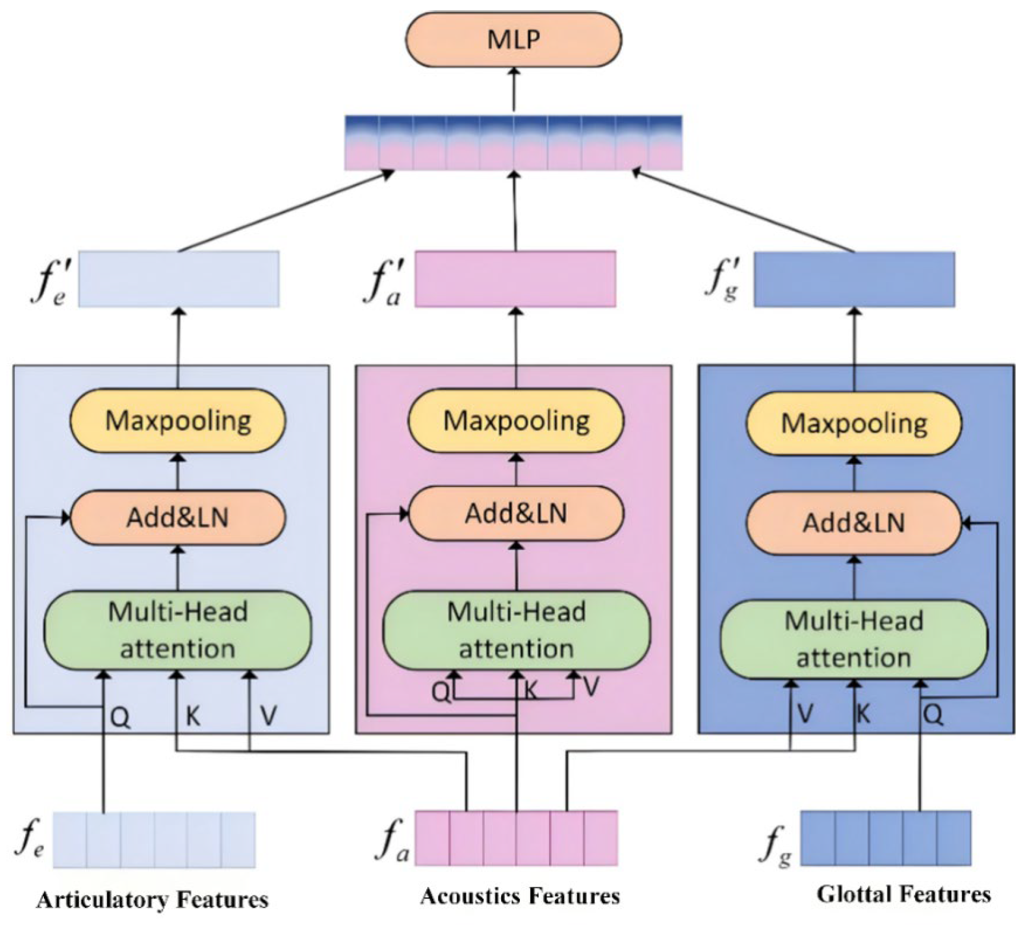
Figure 9.
Interactive attention fusion for multimodal integration. The cross-modal multi-head attention model integrates the interaction between acoustic features (as keys/values) and glottal/articulatory kinematics features (as queries). The representations after attention processing are aggregated and concatenated to form a unified fused feature.
Figure 9.
Interactive attention fusion for multimodal integration. The cross-modal multi-head attention model integrates the interaction between acoustic features (as keys/values) and glottal/articulatory kinematics features (as queries). The representations after attention processing are aggregated and concatenated to form a unified fused feature.
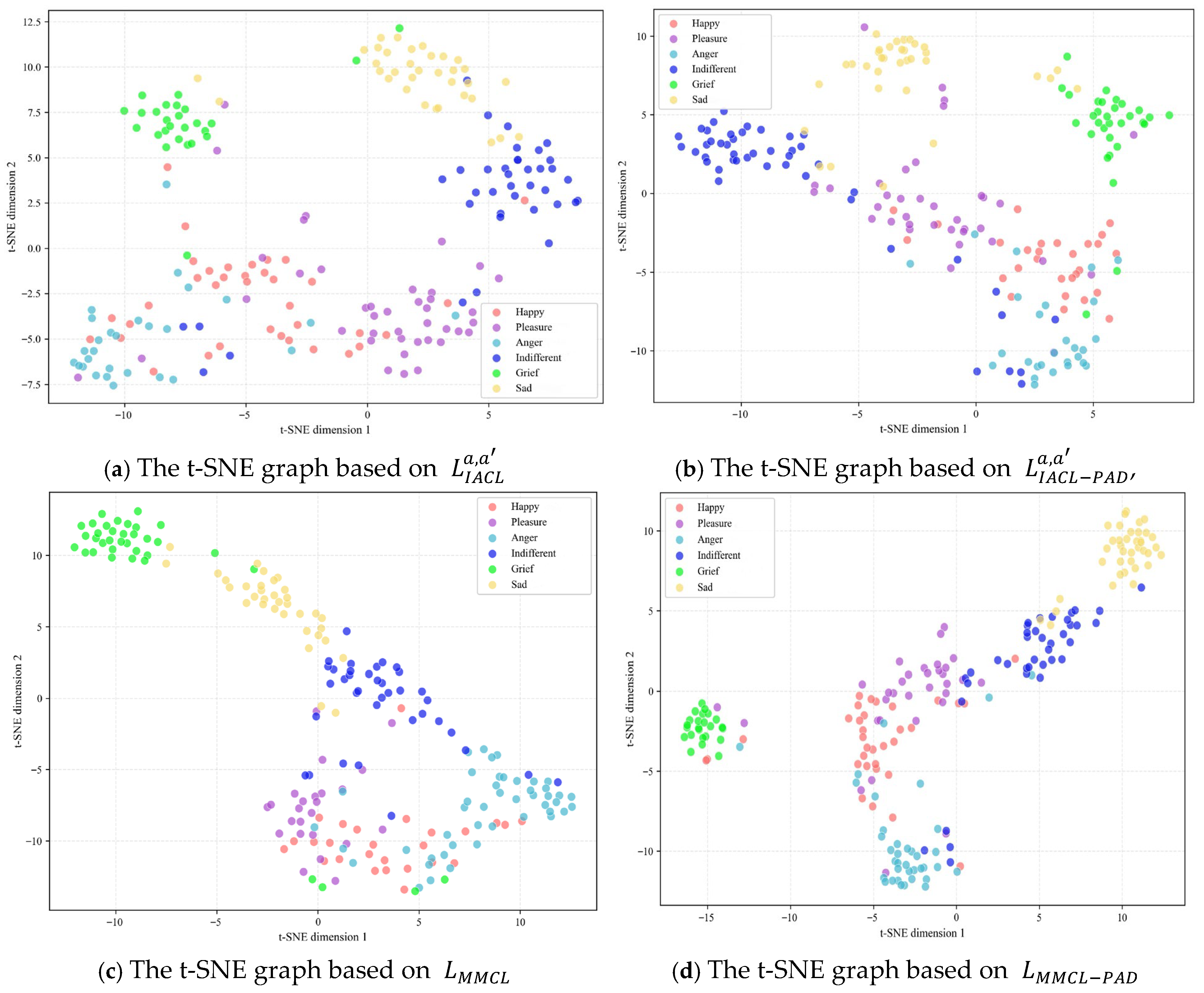
Figure 10.
t-SNE visualization of learned multimodal representations on the STEM-E2VA dataset under different contrastive loss functions: (a) , (b) , (c) , (d) . The points are colored according to their ground-truth emotion labels: red for happy, purple for pleasure, cyan for anger, dark blue for indifferent, green for grief, and yellow for sad.
Figure 10.
t-SNE visualization of learned multimodal representations on the STEM-E2VA dataset under different contrastive loss functions: (a) , (b) , (c) , (d) . The points are colored according to their ground-truth emotion labels: red for happy, purple for pleasure, cyan for anger, dark blue for indifferent, green for grief, and yellow for sad.
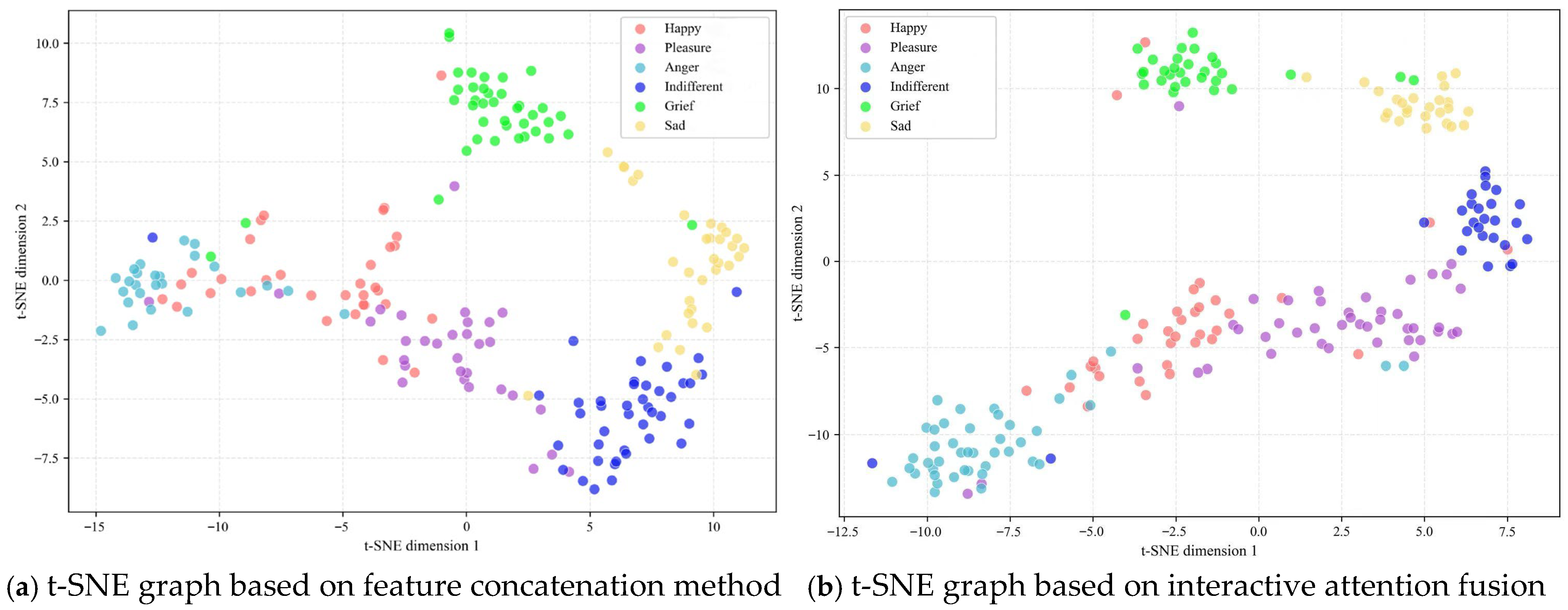
Figure 11.
t-SNE visualization of learned multimodal representations on the STEM-E2VA dataset under different fusion strategies: (a) concatenation method; (b) interactive attention fusion method. The points are colored according to their ground-truth emotion labels: red for happy, purple for pleasure, cyan for anger, dark blue for indifferent, green for grief, and yellow for sad.
Figure 11.
t-SNE visualization of learned multimodal representations on the STEM-E2VA dataset under different fusion strategies: (a) concatenation method; (b) interactive attention fusion method. The points are colored according to their ground-truth emotion labels: red for happy, purple for pleasure, cyan for anger, dark blue for indifferent, green for grief, and yellow for sad.
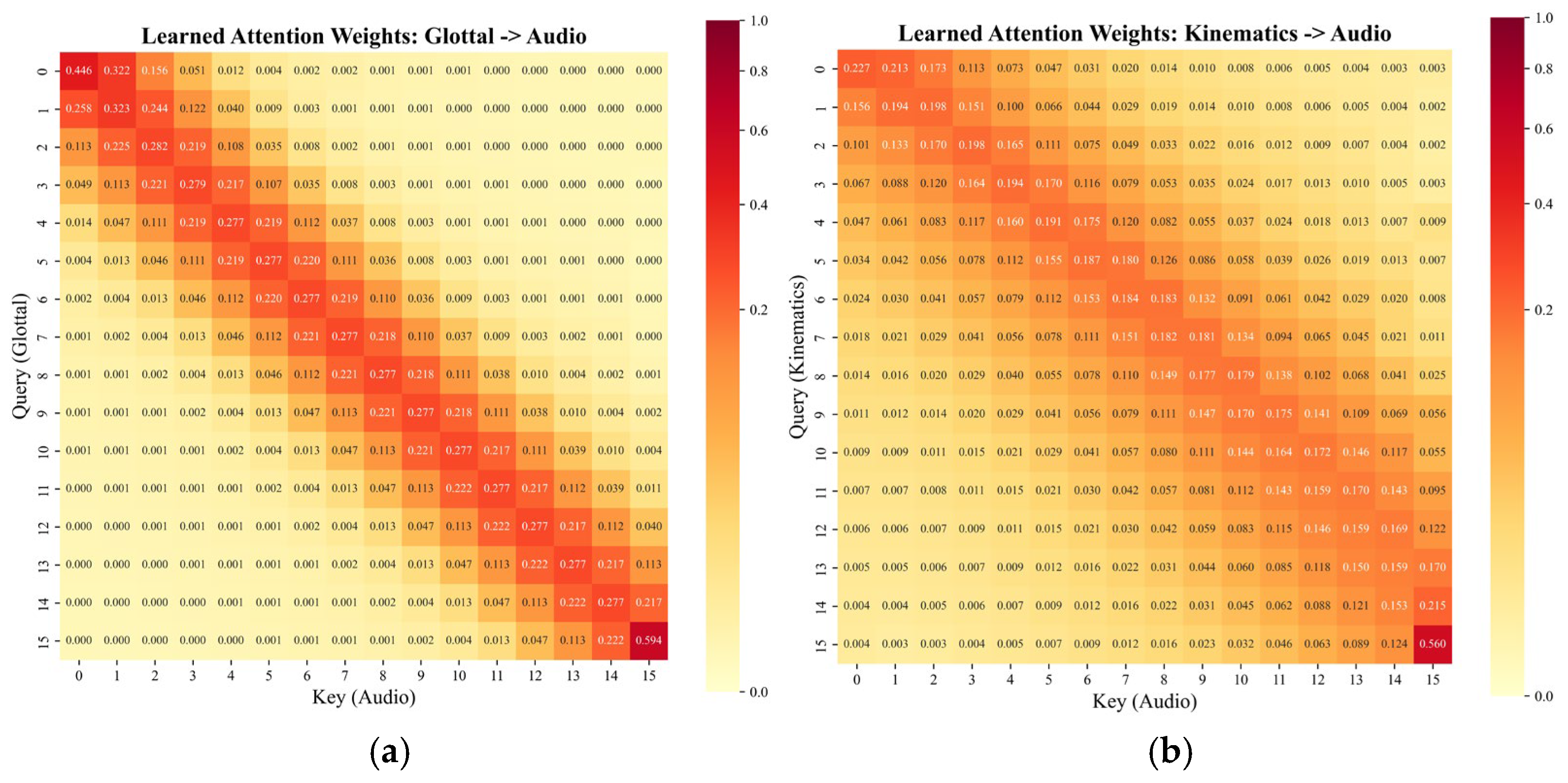
Figure 12.
Visualization of the cross-modal cross-attention weights (averaged over 8 heads) in the interactive fusion module. The horizontal axis denotes the acoustic tokens (keys/values), while the vertical axis denotes the glottal tokens (left) and articulatory kinematics tokens (right) as queries. Each row is normalized to sum to one. The prominent near-diagonal bands suggest that the model captures near-synchronous temporal correspondence and semantic alignment between heterogeneous modalities. (a) Cross-modal interaction attention weight heatmap of “Glottal” → “Audio” (average of 8 heads). (b) Cross-modal interaction attention weights heatmap for “Kinematics → Audio” (average of 8-head model).
Figure 12.
Visualization of the cross-modal cross-attention weights (averaged over 8 heads) in the interactive fusion module. The horizontal axis denotes the acoustic tokens (keys/values), while the vertical axis denotes the glottal tokens (left) and articulatory kinematics tokens (right) as queries. Each row is normalized to sum to one. The prominent near-diagonal bands suggest that the model captures near-synchronous temporal correspondence and semantic alignment between heterogeneous modalities. (a) Cross-modal interaction attention weight heatmap of “Glottal” → “Audio” (average of 8 heads). (b) Cross-modal interaction attention weights heatmap for “Kinematics → Audio” (average of 8-head model).
Table 1.
Discrete emotion categories in STEM-E2VA, comprising neutral and strong/weak intensities of happy, anger, and sad.
Table 1.
Discrete emotion categories in STEM-E2VA, comprising neutral and strong/weak intensities of happy, anger, and sad.
| Neutral | Happy | Anger | Sad |
|---|
| - | Strong | Weak | Strong | Weak | Strong | Weak |
| - | Happy | Pleasure | Anger | Indifference | Grief | Sadness |
Table 2.
Sampling rates, synchronization methods, and alignment strategies across modalities.
Table 2.
Sampling rates, synchronization methods, and alignment strategies across modalities.
| Modality | Acquisition Sampling Rate | Synchronization Strategy | Preprocessing Rate | Input Sequence Length (per 3.4 s Window) | Alignment Mechanism |
|---|
| Acoustic | 48 kHz | Hardware Trigger (Sync Box) | 16 kHz | 54,400 samples | Implicit (via Wav2Vec 2.0 encoder) |
| Glottal | 44.1 kHz | Waveform Alignment (Right-channel) | 16 kHz | 54,400 samples | Implicit (via Wav2Vec 2.0 encoder) |
| Articulatory kinematics | 250 Hz | Hardware Trigger (Sync Box) | 250 Hz | ~850 samples | Explicit (via Cross-Attention) |
Table 3.
Composition of the STEM-E2VA corpus. Counts are reported for rhymes (single rhymes, compound rhymes, and nasal) and sentence prompts across the discrete categories listed in the table (neutral, happy, pleasure, anger, indifference, grief and sadness), together with the total video data duration.
Table 3.
Composition of the STEM-E2VA corpus. Counts are reported for rhymes (single rhymes, compound rhymes, and nasal) and sentence prompts across the discrete categories listed in the table (neutral, happy, pleasure, anger, indifference, grief and sadness), together with the total video data duration.
| Data Type | Type of Corpus | Number of Corpus | Total |
|---|
Pronunciation Data
Acoustic Data
Laryngeal data | Rhymes | Single Rhymes | Compound Rhymes | Nasal | 528 |
| 132 | 198 | 198 |
| Sentence | Neutral | Happy | Pleasure | Anger | Indifference | Grief | Sadness | 2415 |
| 352 | 335 | 345 | 345 | 352 | 337 | 349 |
| Video data | 24.5 h | 24.5 h |
Table 4.
Simplified 7-point PAD annotation scale used in STEM-E2VA. Each dimension (pleasure, arousal, dominance) is rated from 1 to 7 using a semantic differential scheme adapted from the revised PAD scale.
Table 4.
Simplified 7-point PAD annotation scale used in STEM-E2VA. Each dimension (pleasure, arousal, dominance) is rated from 1 to 7 using a semantic differential scheme adapted from the revised PAD scale.
| Meaning | 1 | 2 | 3 | 4 | 5 | 6 | 7 |
|---|
| Pleasure | Angry | Angry | Unpleasant | Neutral | Attentive | Concern | Interested |
| Pejorative | Cold | Calm | Neutral | Mild | Friendly | Intimate |
| Grief | Sad | Perturbed | Neutral | Satisfied | Satisfied | Delighted |
| Infuriated | Sorrow | Boredom | Neutral | Pleasant | Happy | Excited |
| Arousal | Sleepy | Lazy | Absent-minded | Neutral | Advertent | Attentive | Sober |
| Calm | Relaxed | Mild | Neutral | Interested | Cheerful | Excited |
| Depressed | Relaxing | Peaceful | Neutral | Comfortable | Attention-grabbing | Interested |
| Restrained | Scared | Worried | Neutral | Stunned | Surprised | Surprised |
| Dominance | Controlled | Anxious | Perturbed | Neutral | Satisfied | Exhilarating | Mastered |
| Compliant | Accepted | Agreed | Neutral | Hopefully | Covetous | Dominative |
| Humility | Shy | Dependent | Neutral | Confident | Conceited | Proud |
| Affected | Helpless | Accepted | Neutral | Calmly | Attention-grabbing | Influential |
Table 5.
High/low grouping of emotions. Emotions are categorized as high or low along each PAD dimension (pleasure, arousal, dominance).
Table 5.
High/low grouping of emotions. Emotions are categorized as high or low along each PAD dimension (pleasure, arousal, dominance).
| Dimension | Strength | Emotion |
|---|
| Pleasure | High | Happiness, Pleasure |
| Low | Anger, Indifference, Grief, Sadness |
| Arousal | High | Happiness, Pleasure, Anger, Indifference |
| Low | Grief, Sadness |
| Dominance | High | Happiness, Pleasure, Anger, Indifference |
| Low | Grief, Sadness |
Table 6.
Stepwise regression model fit for predicting high-pleasure outlier rates from SCL-90 factors. R, R2, adjusted R2, and the standard error are reported for Models 1–3.
Table 6.
Stepwise regression model fit for predicting high-pleasure outlier rates from SCL-90 factors. R, R2, adjusted R2, and the standard error are reported for Models 1–3.
| Model | R | R2 | Adjusted R2 | Error of Standard Estimation |
|---|
| 1 | 0.762 | 0.581 | 0.558 | 0.094 |
| 2 | 0.826 | 0.682 | 0.644 | 0.084 |
| 3 | 0.894 | 0.799 | 0.762 | 0.069 |
Table 7.
Regression coefficients for model 3 explaining high-pleasure outlier rates. Unstandardized/standardized coefficients, t-statistics, p-values, and collinearity diagnostics (Tolerance, VIF) are reported.
Table 7.
Regression coefficients for model 3 explaining high-pleasure outlier rates. Unstandardized/standardized coefficients, t-statistics, p-values, and collinearity diagnostics (Tolerance, VIF) are reported.
| Model 3 | Unstandardized | Standardized | t | p | Covariance Statistics |
|---|
| Coefficient | Coefficient | Tolerance | VIF |
|---|
| Constant | 0.093 | - | 3.304 | 0.004 | - | - |
| 0.398 | 0.786 | 4.835 | 0.000 | 0.475 | 2.106 |
| −0.328 | −0.790 | −4.146 | 0.001 | 0.345 | 2.895 |
| 0.286 | 0.655 | 3.061 | 0.007 | 0.274 | 3.654 |
Table 8.
Representative PAD vectors for each emotion category after outlier processing. Mean and standard deviation (mean, Std) are reported for pleasure, arousal, and dominance.
Table 8.
Representative PAD vectors for each emotion category after outlier processing. Mean and standard deviation (mean, Std) are reported for pleasure, arousal, and dominance.
| (Mean, Standard Deviation) |
|---|
| Emotion | Pleasure | Arousal | Dominance |
|---|
| Happy | (5.71, 1.01) | (5.77, 0.78) | (5.68, 0.76) |
| Pleasure | (5.26, 0.83) | (5.42, 0.65) | (5.33, 0.63) |
| Anger | (2.04, 0.84) | (6.06, 0.82) | (5.99, 0.79) |
| Indifferent | (2.81, 0.70) | (3.95, 1.12) | (4.14, 1.07) |
| Grief | (1.59, 0.64) | (2.92, 0.38) | (1.65, 0.72) |
| Sadness | (2.38, 0.60) | (2.24, 0.74) | (2.45, 0.79) |
Table 9.
Single-modality emotion recognition baselines on STEM-E2VA. Accuracy (%) is reported for acoustic, glottal, and articulatory kinematics modalities using SVM, DNN, and CNN classifiers under the same train/test split.
Table 9.
Single-modality emotion recognition baselines on STEM-E2VA. Accuracy (%) is reported for acoustic, glottal, and articulatory kinematics modalities using SVM, DNN, and CNN classifiers under the same train/test split.
| Modality Type | Model Type | Accuracy |
|---|
| acoustic | SVM | 82.57% |
| DNN | 85.28% |
| CNN | 79.85% |
| glottal | SVM | 72.28% |
| DNN | 79.85% |
| CNN | 65.42% |
| articulatory kinematics | SVM | 53.57% |
| DNN | 61.17% |
| CNN | 52.28% |
Table 10.
Hyperparameter configuration for the four-stage training pipeline. stage 1 pre-trains feature encoders, stage 2 performs contrastive learning, stage 3 jointly trains the multimodal fusion model, and stage 4 fine-tunes downstream classification/regression heads.
Table 10.
Hyperparameter configuration for the four-stage training pipeline. stage 1 pre-trains feature encoders, stage 2 performs contrastive learning, stage 3 jointly trains the multimodal fusion model, and stage 4 fine-tunes downstream classification/regression heads.
| Hyperparameter | Stage 1: Feature
Extraction | Stage 2: Contrastive Learning | Stage 3: Multimodal Joint Training | Stage 4: Downstream Task |
|---|
| Batch size | 32 | 128 | 64 | 64 |
| Learning rate | 0.0001 | 0.001 | 0.001 | 0.001 |
| Optimizer | Adam | SGD (momentum = 0.8) | Adam | Adam |
| Weight decay | 0.0001 | 0.001 | 0.001 | 0.001 |
| LR scheduler | StepLR (step = 50, γ = 0.1) | StepLR (step = 60, γ = 0.1) | StepLR (step = 40, γ = 0.1) | StepLR (step = 50, γ = 0.1) |
| Epoch | 100 | 100 | 80 | 300 |
Table 11.
A comparative experiment on the handling of abnormal values of PAD on STEM-E2VA (original labels and processed labels). Accuracy refers to discrete emotion classification; RMSE-P/A/D represent the regression errors in terms of pleasure, arousal, and dominance.
Table 11.
A comparative experiment on the handling of abnormal values of PAD on STEM-E2VA (original labels and processed labels). Accuracy refers to discrete emotion classification; RMSE-P/A/D represent the regression errors in terms of pleasure, arousal, and dominance.
| Setup | Outlier Processing | Accuracy | RMSE |
|---|
| P | A | D |
|---|
| Baseline (Raw) | unprocessed | 81.61% | 0.129 | 0.124 | 0.481 |
| Proposed | processed | 85.47% | 0.082 | 0.074 | 0.302 |
Table 12.
Effect of multi-scale contrastive learning on STEM-E2VA. We compare intra-modal contrastive learning with the proposed hybrid intra- and inter-modal strategy. Accuracy and RMSE-P/A/D are reported.
Table 12.
Effect of multi-scale contrastive learning on STEM-E2VA. We compare intra-modal contrastive learning with the proposed hybrid intra- and inter-modal strategy. Accuracy and RMSE-P/A/D are reported.
| Dataset | Losses | Accuracy | RMSE |
|---|
| P | A | D |
|---|
| STEM-E2VA | | 76.25% | 0.189 | 0.181 | 0.369 |
| 78.36% | 0.183 | 0.178 | 0.363 |
Table 13.
Effect of incorporating PAD perception into contrastive learning. Comparing PAD-unaware and PAD-aware losses on IEMOCAP and STEM-E2VA yields accuracy and RMSE-P/A/D.
Table 13.
Effect of incorporating PAD perception into contrastive learning. Comparing PAD-unaware and PAD-aware losses on IEMOCAP and STEM-E2VA yields accuracy and RMSE-P/A/D.
| Dataset | Losses | Accuracy | RMSE |
|---|
| P | A | D |
|---|
| IEMOCAP | | 73.63% | 0.236 | 0.253 | 0.402 |
| 74.85% | 0.202 | 0.213 | 0.391 |
| STEM-E2VA | | 76.25% | 0.189 | 0.181 | 0.369 |
| 78.14% | 0.172 | 0.162 | 0.364 |
| 78.36% | 0.183 | 0.178 | 0.363 |
| 81.23% | 0.152 | 0.145 | 0.358 |
Table 14.
Modality ablation on STEM-E2VA. Performance is reported for acoustics alone and progressively adding glottal and articulatory kinematics to quantify each modality’s contribution; accuracy and RMSE-P/A/D are reported.
Table 14.
Modality ablation on STEM-E2VA. Performance is reported for acoustics alone and progressively adding glottal and articulatory kinematics to quantify each modality’s contribution; accuracy and RMSE-P/A/D are reported.
| Modality Combination | Accuracy | RMSE |
|---|
| P | A | D |
|---|
| acoustics | 78.14% | 0.172 | 0.162 | 0.364 |
| Acoustics + glottal | 82.12% | 0.150 | 0.121 | 0.350 |
| Acoustics + articulatory kinematics | 82.51% | 0.144 | 0.135 | 0.342 |
| Acoustics + articulatory kinematics + glottal | 85.47% | 0.082 | 0.074 | 0.302 |
Table 15.
Comparison of fusion method on STEM-E2VA. Simple concatenation is compared with the proposed interactive attention fusion under the same encoders and training protocol; accuracy and RMSE-P/A/D are reported.
Table 15.
Comparison of fusion method on STEM-E2VA. Simple concatenation is compared with the proposed interactive attention fusion under the same encoders and training protocol; accuracy and RMSE-P/A/D are reported.
| Fusion Method | Accuracy | RMSE |
|---|
| P | A | D |
|---|
| Concatenation | 82.53% | 0.140 | 0.134 | 0.348 |
| Interactive Attention Fusion | 85.47% | 0.082 | 0.074 | 0.302 |
Table 16.
Performance comparison with baseline methods on the IEMOCAP dataset (acoustic only). Accuracy and RMSE-P/A/D are reported.
Table 16.
Performance comparison with baseline methods on the IEMOCAP dataset (acoustic only). Accuracy and RMSE-P/A/D are reported.
| Dataset | Methods | Accuracy | RSME |
|---|
| P | A | D |
|---|
| IEMOCAP | P-TAPT [47] | 74.30% | 0.214 | 0.225 | 0.403 |
| NCDE Classifier [48] | 74.18% | 0.229 | 0.231 | 0.408 |
| Emotion2vec [49] | 74.48% | 0.215 | 0.228 | 0.398 |
| Ours | 74.85% | 0.202 | 0.213 | 0.391 |
Table 17.
Comparison with multimodal fusion baselines on STEM-E2VA. (acoustic, glottal, kinematic); accuracy and RMSE-P/A/D are reported.
Table 17.
Comparison with multimodal fusion baselines on STEM-E2VA. (acoustic, glottal, kinematic); accuracy and RMSE-P/A/D are reported.
| Dataset | Methods | Accuracy | RSME |
|---|
| P | A | D |
|---|
| STEM-E2VA | MulT (MultimodalTranformer) [5] | 82.70 | 0.098 | 0.092 | 0.322 |
| MISA (Modality-Invariant and Specific Representations) [6] | 82.95 | 0.094 | 0.086 | 0.315 |
| HRG-SSA [7] | 83.09% | 0.094 | 0.086 | 0.315 |
| MTAMW [8] | 84.76% | 0089 | 0.081 | 0.307 |
| Ours | 85.47 | 0.082 | 0.074 | 0.302 |




 ,
,