Article

Introducing Friction of Space into the Geography of Cultural Consumption

by
Lorenzo Biferale
1,2,*,
Alessandro Crociata
1,
Lavinia Rossi Mori
2,3,4,5,
Claudio Chiappetta
4 and
Matteo Bruno
2,3
1
Department of Philosophical, Pedagogical and Economic-Quantitative Sciences, University of Chieti-Pescara, Viale Pindaro, 42, 65127 Pescara, Italy
2
Centro Ricerche Enrico Fermi (CREF), Via Panisperna 89/A, 00184 Rome, Italy
3
Sony Computer Science Laboratories—Rome, Joint Initiative CREF-SONY, Centro Ricerche Enrico Fermi, Via Panisperna 89/A, 00184 Rome, Italy
4
Physics Department, Sapienza University of Rome, Piazzale Aldo Moro, 2, 00185 Rome, Italy
5
Physics Department, Università di Roma Tor Vergata, 00133 Rome, Italy
*
Author to whom correspondence should be addressed.
Urban Sci. 2025, 9(8), 316; https://doi.org/10.3390/urbansci9080316
Submission received: 4 June 2025 / Revised: 28 July 2025 / Accepted: 7 August 2025 / Published: 12 August 2025

Abstract

This paper contributes to research on the geography of cultural sectors by exploring cultural consumption habits from a spatial perspective. The study introduces a novel method to the study of cultural consumption spatial patterns by using human mobility data (GPS) to overcome the lack of traditional data on cultural consumption. The results reveal the emergence of spatial inequalities both in the distribution of cultural amenities and in individual consumption behaviours. It shows that proximity to cultural amenities describes individual consumption patterns through a negative power law function, and that this relation is stronger for individuals averse to cultural consumption.

1. Introduction

The cultural economy has acquired a focal role in local and regional development policies during the last decades. The supposed socioeconomic benefits of cultural blossoming in urban settings paved the way for an intense ready-made blueprint for policy setting. Florida’s creative class theory [1], which dominated the scene of urban policies for decades, is nowadays criticised for its mono-directional causal links in domains where socioeconomic complexity cannot be disregarded [2,3]. One of the main criticisms is tracing back the underlying causal scheme to a sort of post-industrial Keynesianism, where the economy of culture causes a boost of demand in the urban system [4]. Escaping from a reductionist treatment of culture as having a mere multiplier effect on the urban economy, scholars have drawn attention to the interplay between the cultural economy and the geographical issues of location, space, and place [5]. By moving from the “cultural turn” [6], scholars have engaged with cultural economic geographies epistemologically, theoretically, empirically, and methodologically [7].
Many of the contributions addressing the geography of cultural phenomena deal with issues of equitable accessibility of cultural amenities, highlighting prominent spatial inequality patterns such as core–periphery [8] and inter-neighbourhood disparities [9]. Great attention has been focused on the supply dimension of culture [10], namely the relevance of cultural amenities to workers’ location choices [11], as well as the impact of cultural heritage on households’ location choices [12]. As for the demand side, there is a dearth of studies focusing on the spatial dimensions of inequality in the geography of cultural amenities [8] and the subsequent spatial participation patterns of individuals residing in different places [13]. While some studies have started to incorporate spatial dimensions in the analysis of cultural consumption behaviours [14,15,16], the geographical distance between consumers and suppliers is either not taken into account or is analysed exclusively in terms of its effect on the probability of consuming culture, due to the limitations of using survey data and probit [17] or logit [16] regression models. Therefore, these studies lack the possibility of exploring the barrier created by spatial distance on an individual’s intensity of cultural consumption.
This paper advocates for a better understanding of the relationship between geography and cultural consumption as a complex system. By conceptualising and operationalising the friction created by spatial distance, the paper addresses the question of understanding the effect of the geographical distance between consumers and suppliers on individual cultural consumption levels.
This study introduces for the first time the use of non-traditional data, namely high-frequency location-based (HFLB—commonly known as GPS) information on human mobility patterns towards cultural amenities, as a way to proxy individual levels of cultural consumption. In this study, high-frequency location-based data (HFLB) refers to anonymised geospatial data collected from GPS-enabled mobile applications that track individuals’ movements over time with high temporal granularity. HFLB data captures user locations at frequent intervals, allowing for the detailed reconstruction of mobility patterns and visits to specific points of interest (POIs).
Although recent scholarship has explored the use of non-traditional data sources to investigate cultural phenomena, such as Spotify listening logs [18], YouTube consumption patterns [19], or user engagement on social media [20], these sources typically lack geographical specificity or spatial continuity. In contrast, high-frequency location-based data (HFLB), such as GPS traces from mobile devices, enable the study of cultural consumption in motion, linking individual behaviours to the geography of residence, urban structure, and travel behaviour. This approach makes it possible not only to identify where cultural consumption occurs, but also to reconstruct the mobility trajectories that precede and follow it, thus offering insights into who consumes culture, from where, and under what spatial constraints. While conventional data sources, such as surveys or ticketing systems, offer static snapshots limited to the moment and site of consumption, HFLB captures real-world behaviour as it unfolds over time and space, overcoming issues of recall bias and sampling limitations [21]. This methodological innovation allows us to operationalise the friction of space and assess how spatial distance and remoteness impact consumption levels. Furthermore, it lays the groundwork for future research on mobility dynamics such as trip chaining and multimodal access, which remain largely invisible to traditional methods and are central to a deeper understanding of spatial inequality in cultural participation.
While this study focuses on cultural consumption, it is important to clarify that the analysis refers specifically to activities linked to the Cultural and Creative Industries (CCIs) and the consumption of market-mediated cultural services. This narrower focus, however, reinforces the analytical strength of our study, which implicitly assumes the existence of market dynamics, enabling us to model spatial consumption behaviours through demand–supply logic.
At the same time, this paper is not only methodologically novel, but also delivers new knowledge regarding the study of cultural consumption in three distinct ways.
First, it shows the potential and the merits of the explored method, which delves deeper at both the spatial and the individual level than traditional data would allow. By using geographical data on human mobility in a continuous spatial setting, we bring out the friction of space, interpreted as the decaying effect that proximity with the offer has on individual cultural consumption levels. Moving away from purely theoretical formulations, through real-world data describing how individuals move around, we show that space no longer needs to be conceptualised as a smooth surface, but as a rough component that plays a significant role in describing human cultural consumption behaviour. We therefore conceptualise the friction of space as the non-linear decrease in the level of cultural consumption corresponding to a marginal increase in the distance between the consumers’ home location and the city’s offer of cultural amenities.
Second, we empirically show that proximity with the cultural offer is positively correlated with individual levels of consumption [13,16], and, by operating in a continuous spatial setting, we advance current knowledge by showing that this relationship is a non-linear one that fades after a given proximity cut-off value, positioned between a travel distance (the measure used for proximity) of 15 and 20 min, resonating therefore with 15 min city theory [22,23]. We further advance the literature by presenting an original classification of individuals to show that the effect played by proximity on consumption levels is significantly stronger for individuals who are averse to cultural consumption compared to individuals who are prone to cultural consumption, signifying that location decisions have lower effects on people with higher human capital.
Third, we operationalise the results by fitting the power law function that best describes the non-linear data correlation. By modelling human behaviour through simple mathematical laws, we show the utility of our method and data, which rely both on the provision of a powerful tool for policy-makers and on its simple scalability. By providing a viable alternative to the need to resort to survey data for cultural consumption research, which is often expensive and time-consuming to collect, and from the potential biases of over/underestimation derived from their use [24], we show the high potential of a method which is smoothly scalable and replicable for evidence-based cultural policies in diverse territorial contexts.
This paper first introduces the most relevant interdisciplinary academic research on cultural consumption and human mobility theories (Section 2). It then moves to formulation of the research questions, most importantly exploration of the possibility of using high-frequency location-based (HFLB) data to understand the complexity of cultural consumption within a geographical perspective. After thoroughly describing the data used for the analysis (Section 3) and the methods adopted (Section 4), Section 5 focuses on analysis of HFLB at the point of origin, the home location of individuals, to investigate the extent to which distance from the city’s cultural supply describes cultural consumption patterns. Afterwards, the main results are discussed (Section 6). The paper concludes by highlighting the most relevant directions for future research stemming from the results obtained.

2. Literature Background

If, on one hand, culture has come to dominate the scene of local development policies as a tool for urban regeneration, on the other hand, as Sacco and Crociata point out [3], current policy models fail to grasp the complexity of cultural and creative phenomena. The popularity of Florida’s approach with policymakers is explained thanks to its ready-to-implement conceptualisation, with the identification of mono-directional causal links. At the same time, as subsequent research has shown, together with poor empirical evidence to support both the existence of a creative class and the hypothesis that creative cities perform better than others [24], it fails to capture both the progressive and problematic contributions of creativity by conflating its complexity with neoliberal urban political regimes [25]. The adoption of mono-directional approaches [26], by failing to capture the underlying social dynamics of the urban contexts in which cultural policies are implemented, might risk generating negative lock-in cycles that exacerbate inequalities.
The necessity of widening participation and increasing access remains the main question of concern, with the aim of making cultural consumption more equitable, calling for cultural mapping approaches able to assess equity of access to bridge the divide between participation and provision [27,28]. Urban planners have placed a strong emphasis on equitable distribution of public facilities, with the assumption that there is a correlation between the location of public facilities and different measures of accessibility [23,29,30]. Such scholars define urban equity as the degree to which public facilities are distributed spatially in an equal way over different areas corresponding to spatial variation in the need for those services [31].
Several studies have therefore addressed the geography of cultural consumption from the supply point of view [32], showing the existence of non-random spatial clustering in the location patterns of cultural amenities and industries [33]. Grodach [34] investigates patterns of spatial concentration of arts industries across different urban areas, as well as the local territorial characteristics associated with artistic clusters [35], finding them to be extremely place-specific. A study that explored patterns of cultural participation of different social groups found that geographic accessibility and commuting patterns are strong predictors of higher attendance levels [36]. Cultural amenity location patterns have also been investigated in terms of neighbourhood characteristics such as racial, income, and industry diversity, finding that more racially diverse and more economically uniform neighbourhoods are the ones that benefit the most from the presence of artistic organisations [37]. Economic geographers have investigated the role played by cultural amenities on workers’ location choices [11], finding that workers are willing to reduce their wages in exchange for better urban amenities, and that such preferences do not differ by skill level. Together with cultural amenities, studies also show that cultural heritage has a significant impact on the attractiveness of cities in terms of households’ location choices [12].
At the same time, there is a lack of studies focusing on cultural consumption through a geographical approach. Some scholars have included geographical dimensions, such as access to the cultural supply, in the explanation of cultural consumption behaviours. This is the case for studies focusing on a city’s specialisation in the creative economy [15] and on a territory’s availability of cultural amenities [17], as well as for studies adopting a neighbourhood approach by including accessibility to public transport and cultural amenities. Nonetheless, the effects of neighbourhood characteristics on cultural consumption have usually been conceptualised as either compositional or contextual [16]; that is, either given by the fact that different territories have different population groups in terms of socio-demographic characteristics that therefore have different patterns of cultural consumption, or resulting from broader territorial characteristics such as access to jobs, transport, or other services [38,39].
Furthermore, most studies adopt what has become a dominant approach in regional science, the discretisation of space in finite space domains [40], departing from classical theories of location and land use that adopted a continuous spatial setting, such as Launhardt [41], Weber [42], and von Thunen [43]. Such an approach is necessary when spatial dimensions (such as access or distance) need to be conflated into models together with other socioeconomic neighbourhood characteristics. The spatial analysis of cultural consumption patterns becomes relevant to uncover patterns of social exclusion, which are now mostly explored aspatially through a sociological lens, following a Bourdieusian approach [44]. This approach has helped to give relevance to cultural consumption as a tool to foster virtuous human behaviours, both at the societal [45,46,47,48] and at the individual level [49,50,51]. Research has addressed the relation between cultural consumption and social stratifications, arguing that culture represents a powerful policy tool to fight social exclusion [52], mostly as a tool to boost prosocial and proactive behaviour [53,54].
Nonetheless, there is a scarcity of studies specifically exploring the problem of inequalities in the geographic distribution of cultural amenities [8] and the subsequent spatial participation patterns of individuals residing in different places [13]. This paper argues for a better understanding of cultural consumption habits in urban contexts, considering the spatial participation patterns of individuals in a continuous spatial setting, with the aim of understanding the effect of the geographical distance between consumers and suppliers on individual cultural consumption levels. In doing so, it explores the potential of using data regarding mobility towards cultural amenities as a measure of physical cultural participation and consumption.
The movement of people is fundamental to our societies, as, among other things, it enables social, economic, and cultural exchanges, shapes the form of cities, gives rise to traffic congestion and pollution, and fuels the spread of contagious diseases [55]. Urban mobility information, operationalised through high-frequency location-based data (HFLB), can be extremely useful in countering the lack of traditional data, such as cultural consumption data, and therefore inform evidence-based policies. Mobility data allows unveiling of the invisible boundaries that segregate people in different groups with diverse accessibility to services [56] and understanding of patterns of spatial segregation at a very granular level [57], thanks to the analysis of visiting rates and distances to different locations within a given area [58]. It is the heterogeneity of trips that dictates the rate at which individuals from different neighbourhoods share the same space and may interact with each other [59], making analysis of mobility patterns towards and visiting frequency of cultural amenities a very effective tool in studying cultural consumption patterns.

3. Data

The amount of digital data logging human mobility traces has boomed in recent years. HFLB has proved to be an extremely valuable source to measure human mobility patterns at unprecedented levels of both spatial and temporal granularity. Such data are usually collected through applications on GPS-enabled phones that register the movement of users in space.

3.1. Data Sources

The mobility data used for this analysis come from users with at least one application using the data provider’s framework on their phone who opted to share anonymised data through a GDPR-compliant process. The dataset contains, for each record, an anonymous ID of the user, latitude and longitude coordinates, and a timestamp with local time and date for all recorded positions. To define the purpose of a stop, the mobility dataset has been enriched with semantic information on the category of the point of interest (POI) where the user makes the stop. This is achieved using open-source data collected from Open Street Map© (OSM) through Overpass API [60]. More specifically, each venue found on OSM has associated metadata (tags) that make it possible to determine the typology and category of the location. OSM tags consist of two elements: a key and a value (usually expressed in the form key.value). The key describes the category, or type of POI, while the value provides further detail. As an example, hospitals can be labelled either as amenity.hospital or building.hospital. In line with the scope of this research, we focus exclusively on cultural POIs associated with cultural and creative industries (CCIs), thus adopting a definition of culture centred on market-oriented consumption and excluding broader non-market cultural practices.

3.2. Data Preparation

Stops are extracted from the mobility dataset according to Hariharan and Toyama [61] by clustering a group of registered positions contiguous in space with a maximum distance between any pair of points less than the diameter D s , for at least a given time T s . The stop duration considered is T s = 600 s, and the stop diameter is D s = 200 m. The stops of each user have been clustered using the DBSCAN algorithm with ε = 100 m (the maximum distance between two points to be considered linked) and s = 1 (the minimum number of neighbours within distance for a point to be regarded as a core point). In other words, stops are extracted by finding clusters of registered positions and are defined as the medoid of the cluster’s positions. We first proceed by assigning home and work locations for each user by considering the 9 p.m. to 8 a.m. hours as home hours on all nights of the week and 9 a.m. to 6:30 p.m. as working hours on weekdays. No minimum duration of home and work stops has been established; the location picked was the one where the user spent the most time in the two time ranges. To reduce data noise, the dataset has been limited to users with at least 15 active days and a minimum of ten valid stops.
Afterwards, third-place stops are given a POI category if they fall within 200 m of an OSM POI. Each POI is beforehand transformed into latitude and longitude coordinates, as OSM POIs can have both point and polygon geometries. For all non-point geometries, we use the barycentre as the projected point. To assign semantic categories to a stop, given the large number of OSM key.value options and the focus of this research being on cultural amenities, we reclassified tags to a simplified taxonomy of places. Considering that currently used taxonomies are mostly focused on the categorisation of cultural production sites, we present a classification derived from the adaptation of the existing ones in the cultural and creative industries (Appendix A), focusing exclusively on OSM tags that represent sites of cultural consumption and which are therefore the potential destination points of cultural trips (Table 1).

3.3. Dataset

The dataset comprises 16,082,194 stops made by 330,929 unique users, covering the period from January 2017 to January 2018. The data are enriched with information from 50,396 OSM POIs (1070 of which are cultural amenities, according to the previously presented semantic classification) that fall within the territory of Milan’s functional urban area (Table 2). The functional urban area of Milan is selected as a case study because it is highly populated, but not too concentrated in the main city; only 43% of the area’s inhabitants live in the city of Milan [62], allowing exploration of both core–periphery and urban–provincial patterns. Furthermore, the city of Milan is considered to be culturally vibrant, with research projects [63] and extensive academic literature on the city’s cultural scene [10,33,64,65] allowing cross-analysis and validation of this paper’s results with previous research.

3.4. Spatial Partitioning

Regarding the chosen spatial partitioning, in order not to lose spatial granularity, a fixed hexagonal tessellation area is preferred for the analysis. Census areas could have been chosen as well, but would have resulted in lower spatial resolution in rural areas. At the same time, regular hexagonal grids face the obstacle of determining a unique size for all areas, which has to be large enough to account for enough people in rural areas while small enough not to account for too many people in urban spaces. No optimal choice for the tessellation size exists, and it depends on the purpose of the analysis. Before choosing the optimal one, the data have been explored using both a hexagonal grid with a 400 m radius and grid with a 2000 m radius, deeming the first more appropriate for this analysis, because it is small enough to capture intra-city differences among neighbourhoods but big enough to aggregate a significant amount of both users’ traces and OSM cultural POIs.
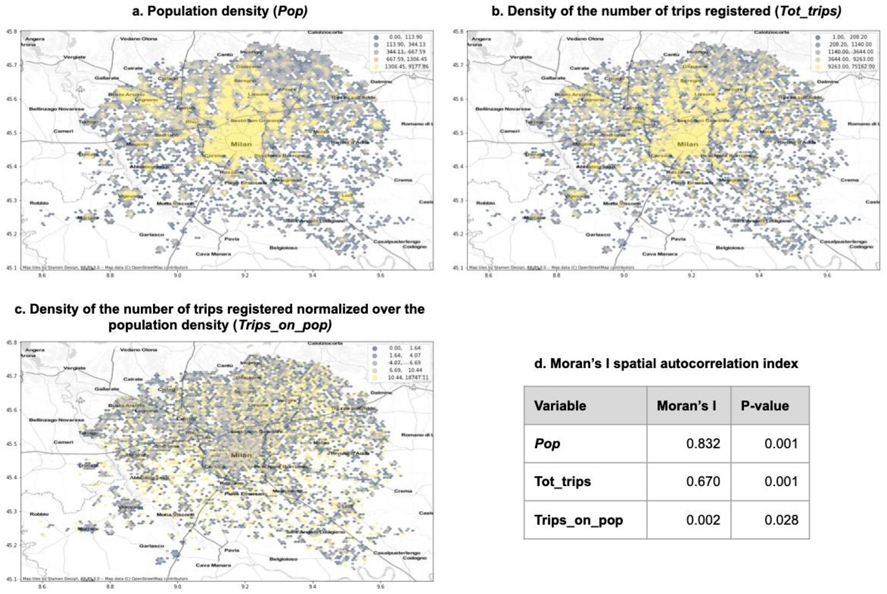
Furthermore, as a preemptive analysis to check for the existence of over/underrepresented areas in the dataset, mapping of the spatial distribution of the HFLB data regarding users’ home location is performed (Appendix B). Both the population (Figure A1a) and the total number of trips recorded per area (Figure A1b) present clear spatial patterns, with a positive, high, and significant spatial autocorrelation index (Figure A1d). At the same time, the ratio between the two values, the per capita density of trips (Figure A1c), and the fact that the results are randomly distributed in Milan’s urban area and not significantly spatially autocorrelated (Figure A1d), allow us to conclude that the data used for the analysis do not present significant spatial biases in terms of over/underrepresented areas.

4. Methods

To perform the analysis, some metrics are computed for each user and averaged for all users with a home location registered within a given hexagon of the tessellation grid. From the HFLB dataset, for each individual it is possible to compute:
  • The overall frequency of cultural consumption (fi), or how many times each individual visited a cultural POI:
    f i = p = 1 N f p , i T i
    where f p , i represents the number of times user i visited cultural amenity p , N   represents the number of cultural amenities visited by user i , and T i represents the number of each individual’s active days.
  • The variety of cultural amenities visited, calculated as the number of different categories of cultural POIs visited by each individual:
    v i = c = 1 N c U c T i
    where U c represents a unique category of cultural amenities visited, N c represents the number of categories visited at least once by user i , and T i represents the number of each individual’s active days.
Frequency ( f i ) and variety ( v i ) metrics are normalised over the number of each individual’s active days, to control for potential distortions that absolute values would have given.
  • The remoteness (Ri) of cultural amenities from the user’s home location, calculated as the average distance of the 20 nearest cultural POIs from the user’s home location.
    R i = p = 1 20 t h i , p 20
    where t h , p represents the time needed to reach the 20 nearest cultural amenities p from the centroid of the hexagon h in which the home location of the user i is registered. Therefore, R i values are the same for all users i with a home location in the same hexagon h , and R i = R h . This remoteness measure is used as a proxy of the average proximity of each neighbourhood with the cultural offer of the city and theoretically derives from the 15 min city theory [23,24]. The travel time is estimated through the OSRM algorithm. The choice of considering the 20 nearest cultural POIs reflects a balance between capturing a representative local offer and ensuring comparability across heterogeneous spatial contexts [66].
Cultural consumption studies point out that indicators of cultural consumption should be able to capture information on the typology of cultural goods consumed, as opposed to the mere quantity of consumption, as this is strongly linked to socioeconomic stratification. In trying to understand how different people appropriate different cultural products [49], it becomes evident how the variety of consumption categories should become the object of measurement, overcoming the distinction between high and low/mass culture [67] and moving towards the integration of different cultural consumption indicators [68]. In this direction, the question which is now being asked is not only whether people have access to facilities, but also what variety of facilities they have access to and what use they make of them [69]. Cultural consumption inequalities have been historically framed by the sociological literature in terms of highbrow and lowbrow products [70], a distinction which is nowadays criticised, as scholars started to point out that modern cultural divisions separate those who have a wide range of cultural interests [71] and a greater tendency towards novelty [72] from those who do not, therefore overcoming traditional cultural hierarchies and framing inequalities from an “access to a variety of products” point of view [73]. To account for such theoretical debates, we propose a compounded measure of the level of consumption ( C i ) which accounts for both quantity and variety factors, measured as visiting POIs that belong to different sub-categories of cultural amenities according to the presented taxonomy (Section 3.2).
C i = f i v i
The new measure of cultural consumption ( C i ), which is correlated to the remoteness of cultural amenities ( R i ), like its two components ( f i , v i ), allows us to control for theoretical debates on how to measure cultural consumption and to update purely quantity-driven indicators ( f i ) with a measure of the typology of culture consumed, implying that the higher the variety ( v i ), the higher the benefits of cultural consumption on the individual.
Once again, to perform a spatial analysis, all variables are aggregated for each hexagonal area of the tessellation grid by averaging the values among all users i with the home location registered in a given hexagon h . As an example, the average level of consumption ( C h ) of each hexagon is obtained through the following equation:
C h =   i   =   1 N i , h C i N i
where N i , h represents the number of users i with a home location registered in hexagon h .
Data on the number of average visits per neighbourhood and their variety in terms of different categories of cultural amenities visited and the average distance travelled by users from the same home hexagon to reach cultural amenities are integrated with information on the proximity of each hexagon to the city’s cultural offer. Individual users are then split in four different categories based on their relative consumption levels and proximity to the cultural offer. This categorisation was performed to explore the extent to which different consumption patterns have different spatial locations within the city.

5. Analysis

By performing a first descriptive analysis (Figure 1), it can be seen that, by increasing remoteness from the city’s cultural offer (3), the average frequency of visits decreases (4). In other words, the more a given place is further away from the city’s cultural offer, the less its residents visit cultural amenities on average. As a robustness check (Figure A2), the same descriptive analysis was performed for the measures of frequency (1) and variety (2) of cultural consumption, obtaining similar results. (Appendix C). Although the relationship between remoteness and cultural participation is continuous, thus preventing identification of a sharp cut-off point, it is possible to observe a distinct change in slope that roughly corresponds to a 15–20 min walking distance, aligning with the widely discussed concept of the “15 min city” [23]. This visual inflection suggests that proximity plays a stronger role in describing consumption patterns within this threshold, beyond which the average frequency of participation appears to decline less markedly.
When mapping the distribution of the hexagonal average of remoteness from the cultural offer and of the level of consumption (5), a clear spatial pattern emerges. Apart from all variables having positive and significant spatial autocorrelation (Figure 2e), a clear core–periphery spatial distribution pattern emerges, resonating with the distribution pattern of the cultural offer (Appendix D). Neighbourhoods (represented by hexagons of the tessellation grid) closer to the centre of urban areas have higher proximity to cultural amenities (Figure 2a) and a higher average level of consumption (Figure 2c). The results reveal core areas with higher levels of consumption and lower remoteness from cultural amenities and an opposite pattern for peripheral areas, with lower levels of consumption and higher remoteness from cultural amenities. The city of Milan is highly unequal, with people in core areas living closer to cultural amenities and consuming more, and people in peripheral areas living further away from cultural amenities and consuming less.
From the visualisations above (Figure 2), it might potentially be inferred that there are two main groups of places in the metropolitan area of Milan:
  • Places on average inhabited by individuals with high consumption levels (4) that are spatially closer to cultural amenities (3), generally concentrated around the core of the main urban centres;
  • Places on average inhabited by individuals with low consumption levels (4) that are spatially far from cultural amenities (3), generally concentrated in the peripheries of the main urban centres.
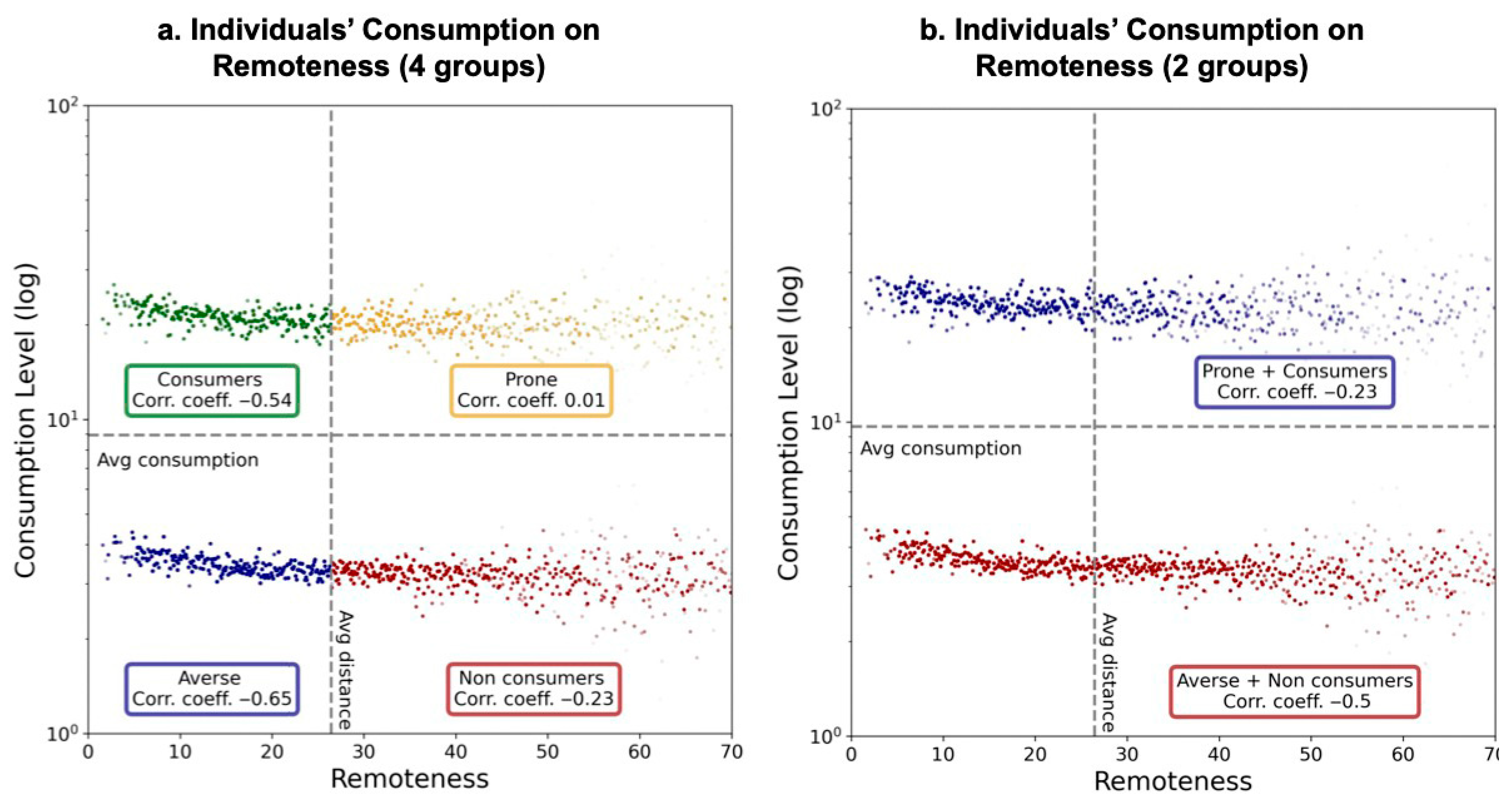
Therefore, the analysis shows how aggregate average results show an apparent mono-directional relationship. At the same time, individual-level data reveal a much fuzzier situation. To better understand such fuzziness, we categorised individuals into four groups based on their relative level of consumption (4) and remoteness (3) from cultural amenities (Figure 3) compared to the sample’s mean. Such classification allows us to better understand the relative composition of each neighbourhood and to explore the extent to which more uniform groups in terms of consumption patterns influence aggregate results.
More precisely, the four groups are:
  • Consumers, behaving according to aggregate flows. Individuals who have consumption levels higher than the sample’s mean and a remoteness from cultural amenities lower than the sample’s mean;
  • Non-consumers, behaving according to aggregate flows. Individuals who have consumption levels lower than the sample’s mean and a remoteness from cultural amenities higher than the sample’s mean;
  • Averse individuals, behaving differently from aggregate flows. Individuals who have consumption levels lower than the sample’s mean and a remoteness from cultural amenities lower than the sample’s mean;
  • Prone individuals, behaving differently from aggregate flows. Individuals who have consumption levels higher than the sample’s mean and a remoteness from cultural amenities higher than the sample’s mean.
When describing the four groups, their composition must be considered first. The majority of individuals (75%) have consumption levels lower than the mean, while only 37% of the sample reflects the expected behaviour, meaning either a low relative consumption level combined with a higher distance from cultural offer or vice versa. Interestingly, the majority of individuals fall in the two non-expected groups, with most of them (45% of the total sample) being culturally averse.
When correlating the remoteness of cultural amenities with the individual level of consumption for the four categories, different relationships emerge (Figure 3a). While all categories have negative correlation coefficients, prone individuals have the lowest coefficient (positive and almost equal to zero), while averse individuals have the highest. This result suggests that the effect of proximity to the cultural offer in increasing the level of individual cultural participation is significantly stronger for those groups of people who are less used to consuming cultural goods (individuals averse to cultural consumption). Similar results are obtained when performing the correlation analysis aggregating individuals in two groups, according to the single criterion of having a cultural consumption level lower ( C i   <   μ C ) or higher ( C i   >   μ C ) than the sample’s mean (Figure 3b). The negative correlation holds true for both groups, but for individuals less accustomed to cultural consumption the correlation is stronger. Visual interpretation of the correlation graphs shows that, for individuals less used to cultural consumption, distance (3) from the city’s cultural amenities describes consumption levels (4) through a strong negative correlation up to a cut-off value, after which the slope of the curve decreases.
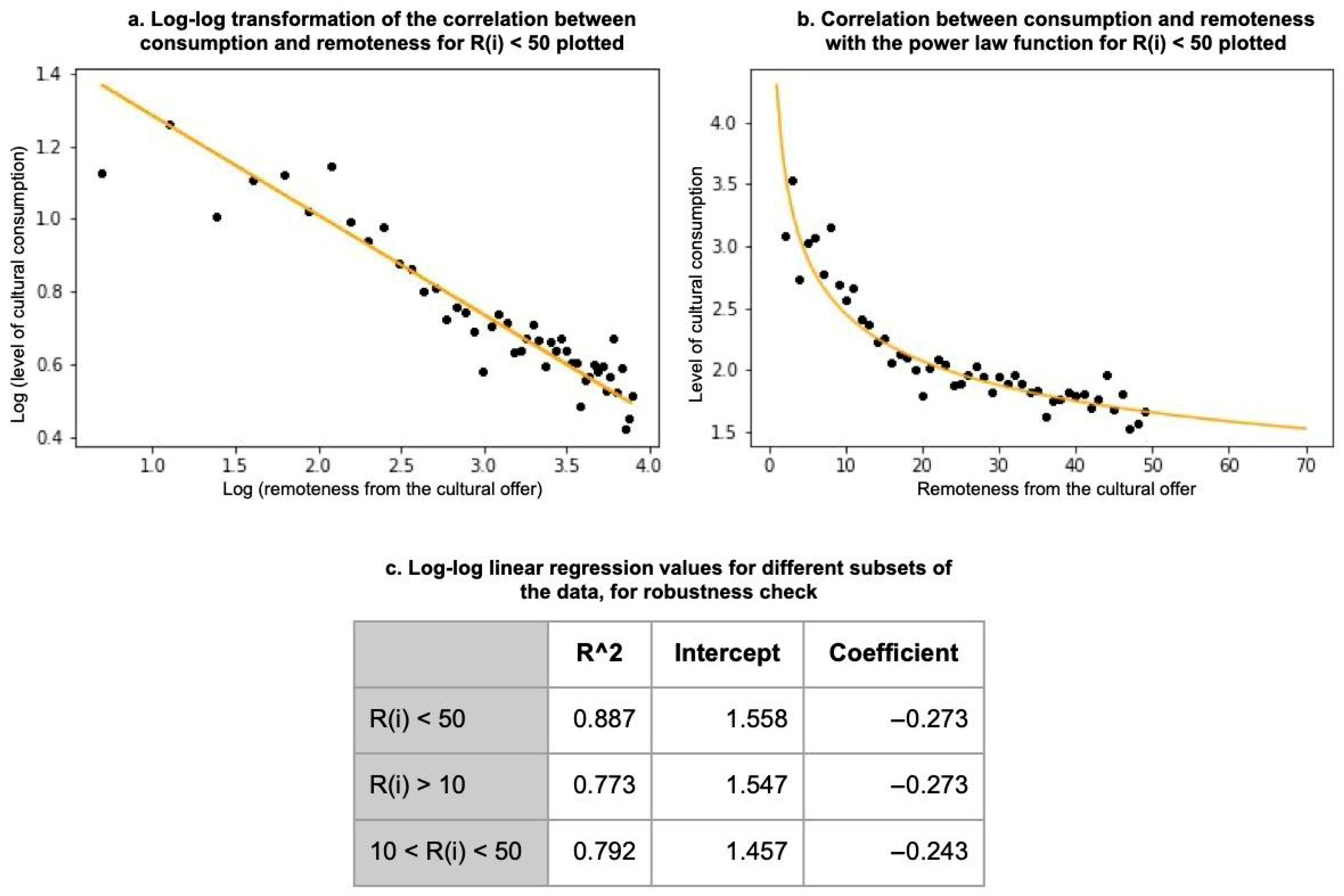
At the same time, it is shown that, by considering all users at the same time, the correlation curve follows a power law function (Figure 4), therefore allowing modelling of cultural consumption levels according to the following equation:
C i   =   α R i β
In a power law function, the relationship between the independent variable ( R ) and the dependent variable ( C ) is non-linear and modelled through an exponent ( β ). Exponent values lower than 1 result in heavy-tailed distributions, where a few values of the independent variable have a significant effect on the dependent one, while the majority of values have relatively little effect. Furthermore, power law functions are found to model real-life phenomena in several domains, from biology to economics, linguistics, and astronomy [75]. In our case, the estimated exponent across all subsets confirms a consistent, sub-linear decay in cultural participation as remoteness increases, implying that a 1% increase in distance leads to a 0.27% decrease in cultural activity.
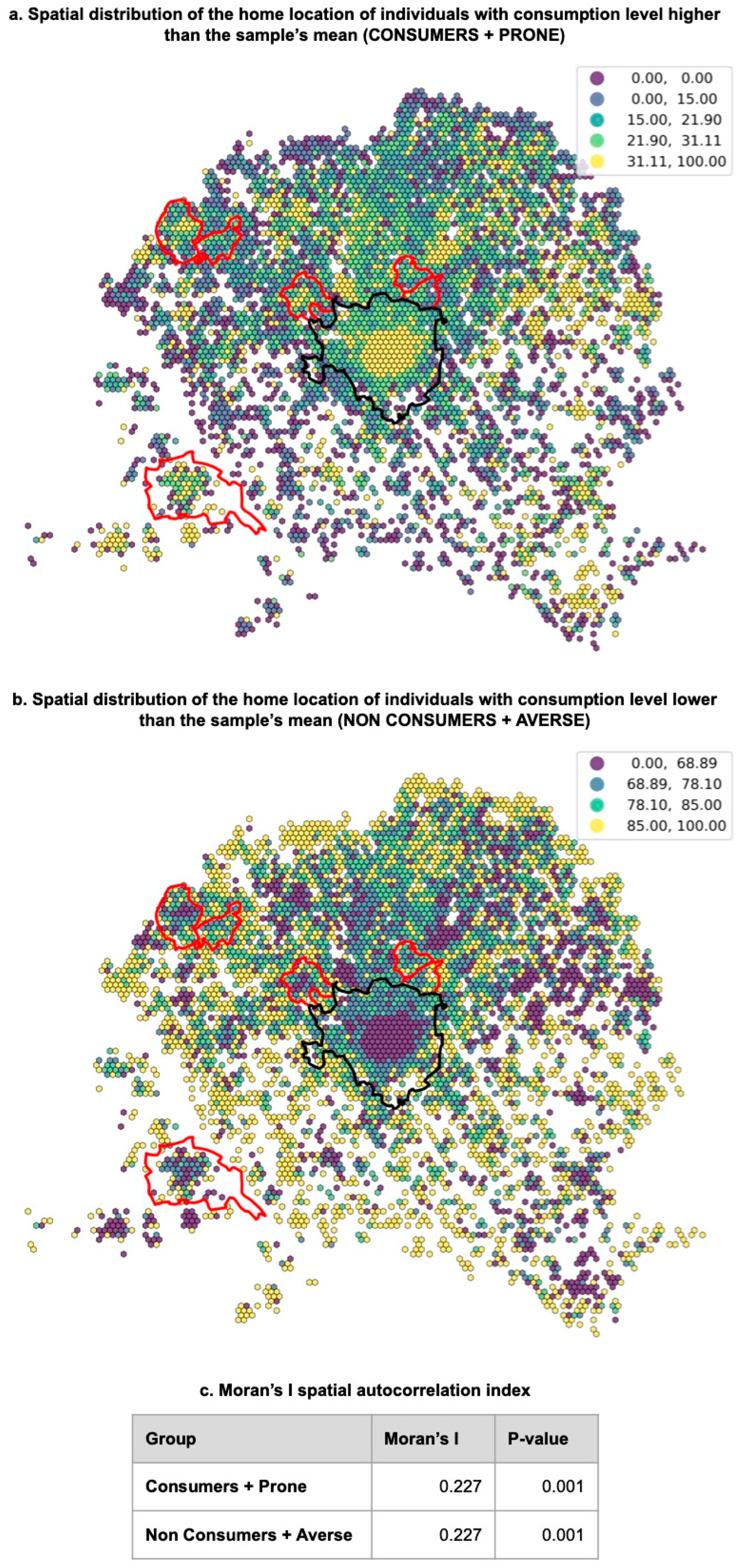
Although aggregated individual data showed an unambiguous pattern, analysis of the disaggregated consumption patterns showed the existence of significant differences in the extent to which remoteness from cultural amenities describes cultural consumption levels among different population groups, each with a more homogenous level of cultural consumption. Such results have particular importance from a policy perspective, mostly through the possibility of mapping the relative presence of each population group in the city’s neighbourhoods to identify areas of higher concentration of each population group, and therefore differentiate policy approaches. Figure 5 shows the relative composition of each hexagon of the tessellation grid. As expected, the same core–periphery patterns previously found are validated, but a closer look at the percentage composition of each neighbourhoods highlights a situation in which individuals more accustomed to cultural consumption make up less than 30% of the population of the majority of the grid, with the exception of core areas in the main urban centres. The same maps show peripheral areas almost entirely inhabited by individuals less used to cultural consumption, reinforcing even more the core–periphery inequality patterns previously identified.

6. Discussion and Conclusions

This paper investigates the way in which individuals move across a city to visit cultural amenities. It argues for the need to develop further knowledge regarding the relationship between geography and cultural consumption as a complex system.
From a methodological standpoint, this study represents a first attempt at using HFLB data to describe spatial patterns of cultural consumption within cities, providing insight into the extent to which human mobility data describe aggregate and individual-level patterns of cultural consumption. The results obtained validate the academic literature on the topic both by showing the emergence of spatial patterns of inequality and by giving them a core–periphery configuration. At the same time, it is shown that HFLB data, while describing aggregate patterns of consumption, allow us to ascertain the variability of such patterns in each neighbourhood, becoming a powerful tool for the formulation of evidence-based local cultural policies and interventions. By combining location-based cluster analysis (Appendix D) with HFLB data describing people’s movements towards cultural amenities, we show that the core–periphery inequality pattern is identifiable both from a supply-side (location of cultural amenities) and a demand-side perspective (people’s consumption patterns from their home location).
This paper’s contribution stems both from its methodological novelty and from three main theoretical advancements. First, it investigates cultural consumption patterns at a deeper level in terms of both geographic and individual granularity than previous studies. By operating in a continuous spatial setting, we identify the decaying effect that proximity with the city’s cultural offer has on individual patterns of consumption, conceptualising it as the friction of space. We show, for the first time on a continuous scale, that space creates friction in the way people are able to appropriate the cultural offer, becoming a relevant determinant of individual consumption patterns.
Second, we validate previous literature on the topic [13,16] through novel data, by showing a positive correlation between proximity to the cultural offer and individual levels of consumption. At the same time, we advance current knowledge of the topic by showing the non-linearity of this relationship and the emergence of a cut-off value. These findings also resonate with the growing policy emphasis on chrono-urbanism [23,24], which shifts the focus from physical proximity to temporal accessibility of urban services. The observed decline in cultural participation beyond a 15–20 min range from cultural amenities supports recent calls to embed time-based metrics into urban and cultural planning strategies [76] that invite planners to consider “temporal distances” as key dimensions of equity and sustainability in service provision, making our findings particularly relevant to current debates on cultural accessibility and the chrono-urbanist framework. We further advance research on the effects of distance on cultural consumption levels by showing that this relationship varies among different categories of individuals. We introduce a novel classification of individuals according to their observed cultural consumption behaviour, showing that, all other conditions being equal, the effects of proximity are stronger for individuals who are less accustomed to cultural consumption.
Third, we operationalise our results by fitting the power law function that best describes cultural consumption behaviours, showing that, through big data, it is possible to describe human behaviours through simple mathematical laws.
While this paper adopts a statistical perspective and focuses on spatial consumption patterns, we acknowledge the importance of situating these findings within the broader context of cultural policy. As clarified in the introduction, this analysis concentrates on cultural amenities that fall within the scope of CCIs, understood in their market-oriented and service-based dimensions. At the same time, the patterns of remoteness and access to cultural amenities we identify have significant implications for the policy design and strategic development of CCIs.
CCIs are increasingly recognised not only for their cultural value, but also for their economic, innovation, and territorial impact. As one of the 14 industrial ecosystems outlined in the European Commission’s Industrial Strategy for Europe, the CCI ecosystem contributes nearly 4% of EU value added and employs around 8 million people, mostly in micro-enterprises and freelance arrangements. These structural features make the sector particularly vulnerable to fragmentation and highly sensitive to spatial disparities in access to infrastructure, audience reach, and cultural demand.
Our findings on spatial remoteness and variation in cultural consumption thus speak directly to one of the key challenges highlighted in EU policy documents: the need for innovation-friendly, territorially balanced infrastructure that can support CCI ecosystems across regions. The observed disparities in access to CCIs can undermine the sector’s contribution to regional competitiveness, particularly where cultural amenities are concentrated in central urban areas, while peripheral zones remain underserved. These dynamics point to the urgency of place-based policies that take into account spatial consumption patterns as part of broader strategies for cultural inclusion and economic diversification.
In this sense, while our analysis adopts a necessarily “reductionist” definition of culture due to data and modelling requirements, it yields insights of relevance for broader policy debates.
Being an exploratory study, this paper’s main limitation resides in the impossibility of drawing causal implications from the obtained results. At the same time, given the anonymity of the HFLB data, it is not possible to control for individual socio-economic and demographic characteristics, which are found to be significant determinants of consumption in the extensive literature on the social stratification of cultural consumption. Notwithstanding their limitations, the obtained results open relevant and interesting possibilities for future research:
  • By using HFLB data on individual mobility towards cultural amenities as a proxy for the level of individual cultural consumption, it is possible to overcome the limitations of traditional survey data [25];
  • By modelling cultural consumption levels through a power law function, it is possible to operationalise the method in different urban and non-urban settings and to understand to what extent metrics such as the slope of the power-law fit (intended as a measure of the sensitivity of cultural consumption levels to spatial friction) are related to broader urban socioeconomic characteristics;
  • By including neighbourhood-specific data on socioeconomic stratification, it is possible to model demand functions for cultural goods in geographical settings;
  • By including individuals’ visiting preferences, it is possible to understand how different neighbourhoods appropriate different types of cultural goods and how such differences influence overall consumption levels;
  • By looking for trip-chaining patterns it is possible to understand the effects of other mobility behaviours, such as recreational or work-related ones, on patterns of cultural consumption.
As a first exploratory descriptive analysis of cultural consumption patterns through a big data approach, this analysis sheds light on a phenomenon in which complexity is paramount. While the methodological approach presented in this paper is scalable and replicable, the findings are derived from the specific context of Milan: a large, culturally vibrant city with relatively well-developed infrastructure and public amenities. As such, the spatial dynamics observed, particularly the patterns of core–periphery inequality and the 15–20 min proximity threshold, may not be directly transferable to smaller or less infrastructure-rich urban areas. Further research is required to assess how different levels of urban infrastructure, density, and public cultural provision influence the relationship between proximity and cultural consumption in diverse city contexts. The conclusions from this study should therefore be interpreted with regard to the characteristics of Milan’s urban fabric.
To conclude, this paper opens the door for a new approach to the exploration of cultural consumption, with the aim of leading towards cultural policies capable of addressing the inner complexity of consumption patterns. As shown, culture within cities is highly spatially unequal. Proximity to cultural amenities represents one of the most easily actionable levers through which policymakers can reduce such inequalities. Understanding the extent to which the location of amenities influences consumption must therefore become a primary research objective, and this paper represents a first step in this direction.

Author Contributions

Conceptualization, L.B.; methodology, L.B., L.R.M., C.C. and M.B.; formal analysis, L.B., L.R.M., C.C. and M.B.; data curation, L.B., L.R.M., C.C. and M.B.; writing—original draft, L.B.; writing—review and editing, L.B., visualization, L.B. and M.B.; supervision, A.C. All authors have read and agreed to the published version of the manuscript.

Funding

This research received no external funding.

Data Availability Statement

The datasets presented in this article are not readily available because of their commercial nature.

Conflicts of Interest

The authors declare no conflict of interest.

Appendix A. Categorising Cultural Amenities

While several taxonomies of cultural and creative industries (CCIs) have already been presented and extensively used, the dynamic and evolving nature of CCIs makes the goal of reaching an exhaustive and conclusive classification an impossible one. Furthermore, to the extent of the authors’ knowledge, current taxonomies address cultural production sites, and a classification of cultural consumption sites has yet to be presented. Therefore, a classification is derived from the adaptation of existing ones on CCIs, limiting its objective to the classification of cultural POIs for the purpose of this project, and not to the proposition of a novel taxonomy of cultural amenities. This classification is limited to cultural amenities associated with cultural and creative industries (CCIs), reflecting a market-oriented definition of culture aligned with the analytical scope of this study, and does not encompass broader non-market cultural expressions such as volunteering, informal practices, or community-based cultural participation.
More precisely, the taxonomies considered (Table A1) all identify the following categories of cultural and creative industries, which have been adopted in the proposed classification, with the following adjustments:
  • Heritage/cultural sites: defined in CCI taxonomies as comprising heritage sites, museums, libraries, and archives, it is split in two main sub-categories, namely heritage and museums, to control for the inclusion of open-air monuments and attractions in the heritage category and their differences from museums.
  • Publishing: libraries and archives are removed from the heritage category and inserted in the new category “reading.”
  • Performing arts/independent artists, writers, and performers: live entertainment is split in two categories, one for theatre and one for night life, which represents concert halls and clubs, as music consumed in theatres is captured by the theatre category.
  • Film/motion picture and video industries: the category is kept as it was in CCI taxonomies, capturing exclusively movie theatres.
Table A1. Classifications of creative industries.
Creative IndustriesDCMS (2009)WIPO (2003)Eurostat LEG (2000)KEA (2006)UNCTAD (2010)DISCE (2022)
Printing X
PublishingXXXXXX
AdvertisingXXXXXX
ArchitectureXXXXXX
Arts marketsXXXXXX
CraftsXXXXXX
DesignXXXXXX
FashionXXXXXX
FilmXXXXXX
MusicXXXXXX
Performing artsXXXXXX
PhotographyXXXXXX
Software and VGXXXXXX
Radio and TVXXXXXX
Heritage XXX
Interactive media XXXX
Other visual arts XX X
Copyright X
Cultural tourism X
Creative R&D XX
Source: Domenech et al. [77] integrated with DISCE [78].
Such changes were necessary to adapt the presented taxonomies, which describe categories of cultural production, to the subject of this paper, which is categories of cultural consumption. Furthermore, it must be pointed out that the presented classification derives from manual analysis of OSM tags and is specifically built to reflect the categorisation that such data allow; it is therefore slightly divergent from taxonomies presented in the considered literature, as it aims to cluster the data for the purposes of this paper rather than propose a novel taxonomy. The categories advertising, architecture, crafts, design, and photography, which were identified by all the considered taxonomies, have been dropped, either because they only describe categories of cultural goods production that have no consumption equivalent (e.g., advertisement), or because they lack the equivalent tag in Open Street Map that allows for identification of POIs.
Initially, three additional categories were created to collect Open Street Map (OSM) tags that remained excluded from the previously mentioned categories; two of them represented more hybrid places of cultural consumption (event and amusement) such as community centres and cultural associations, and one represented tourism accommodation sites. Such categories were later removed from the analysis for their too-fuzzy classification by OSM and/or due to the lack of a significant amount of POIs.

Appendix B. Data Check

Figure A1. Spatial distribution of users’ home locations. The maps show the spatial distribution of the available data over the city of Milan. Values are obtained by averaging individual data over each hexagon of the tessellation grid. (a) Quantile values of the population density according to the ISTAT census. (b) Quantile values of the number of trips registered for users living in a given hexagon. (c) Quantile values of the per capita density of trips registered. (d) Moran’s spatial autocorrelation index for all the variables mapped.
Urbansci 09 00316 g0a1

Appendix C. Cluster Analysis of Cultural Amenities
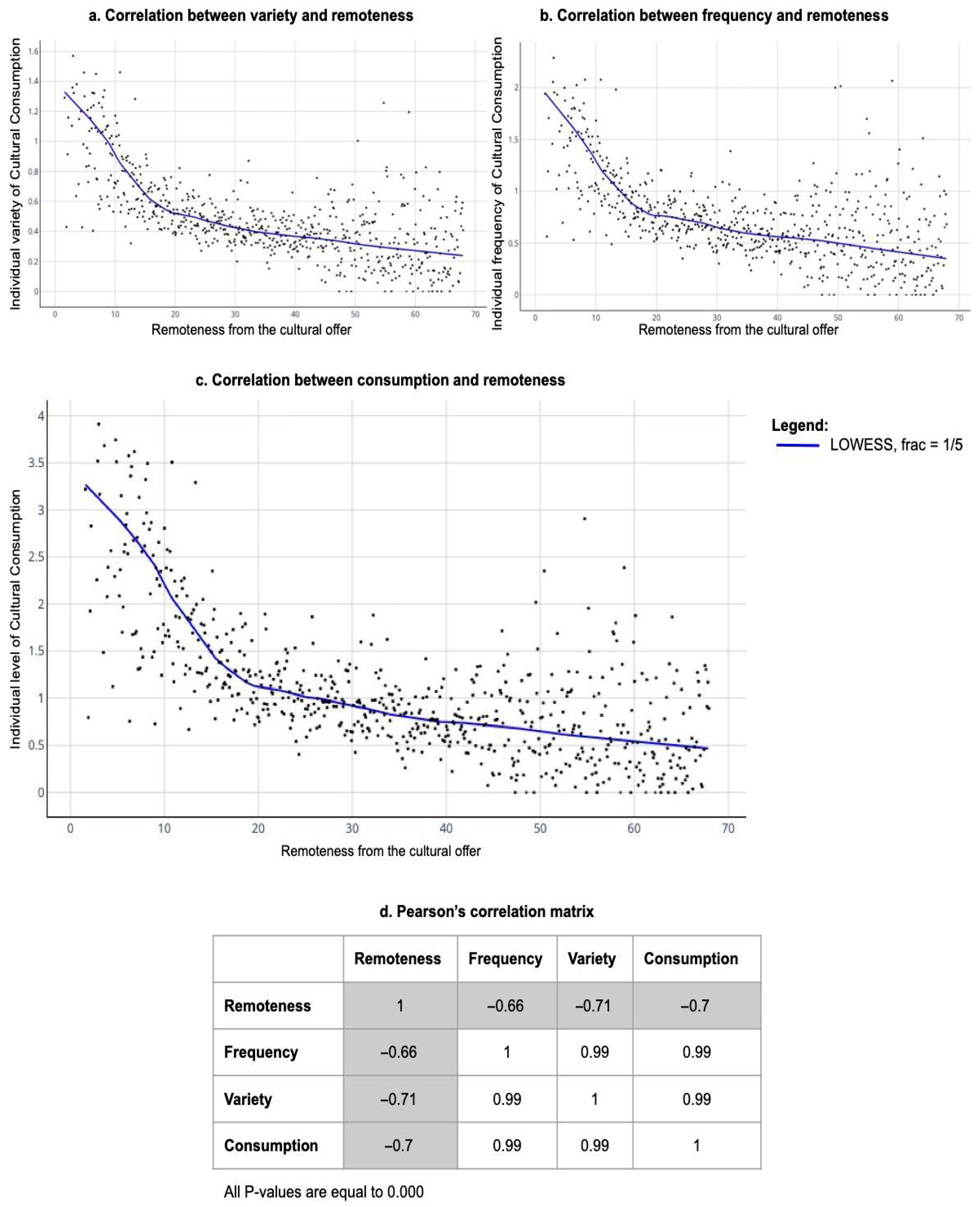
The check the effects on the analysis derived from the adoption of a compounded indicator for individual levels of cultural consumption (4), the descriptive analysis of its correlation with remoteness from the cultural offer (3) has been replicated separately for the measures of frequency (1) and variety (2) of cultural consumption, obtaining similar results.
Figure A2. Correlation of consumption measures with remoteness from cultural amenities. (a) Scatter plot of v i against R i . (b) Scatter plot of f i against R i . (c) Scatter plot of C i against R i . (d) Pearson’s correlation matrix of v i , f i , C i , and R i . The scatter plots show the locally weighted scatterplot smoothing (LOWESS) algorithm, a supervised learning regression algorithm used for regression analysis where data attributes do not allow linear regression models to produce a good fit [74]. Note: to increase the readability of the data visualisations, and to reduce the noise of the data at the users’ level, remoteness values (x) have been rounded (one decimal place), and y variables have been averaged over each rounded x. All correlations hold true for non-rounded and non-averaged values as well.
Urbansci 09 00316 g0a2

Appendix D. Cluster Analysis of Cultural Amenities
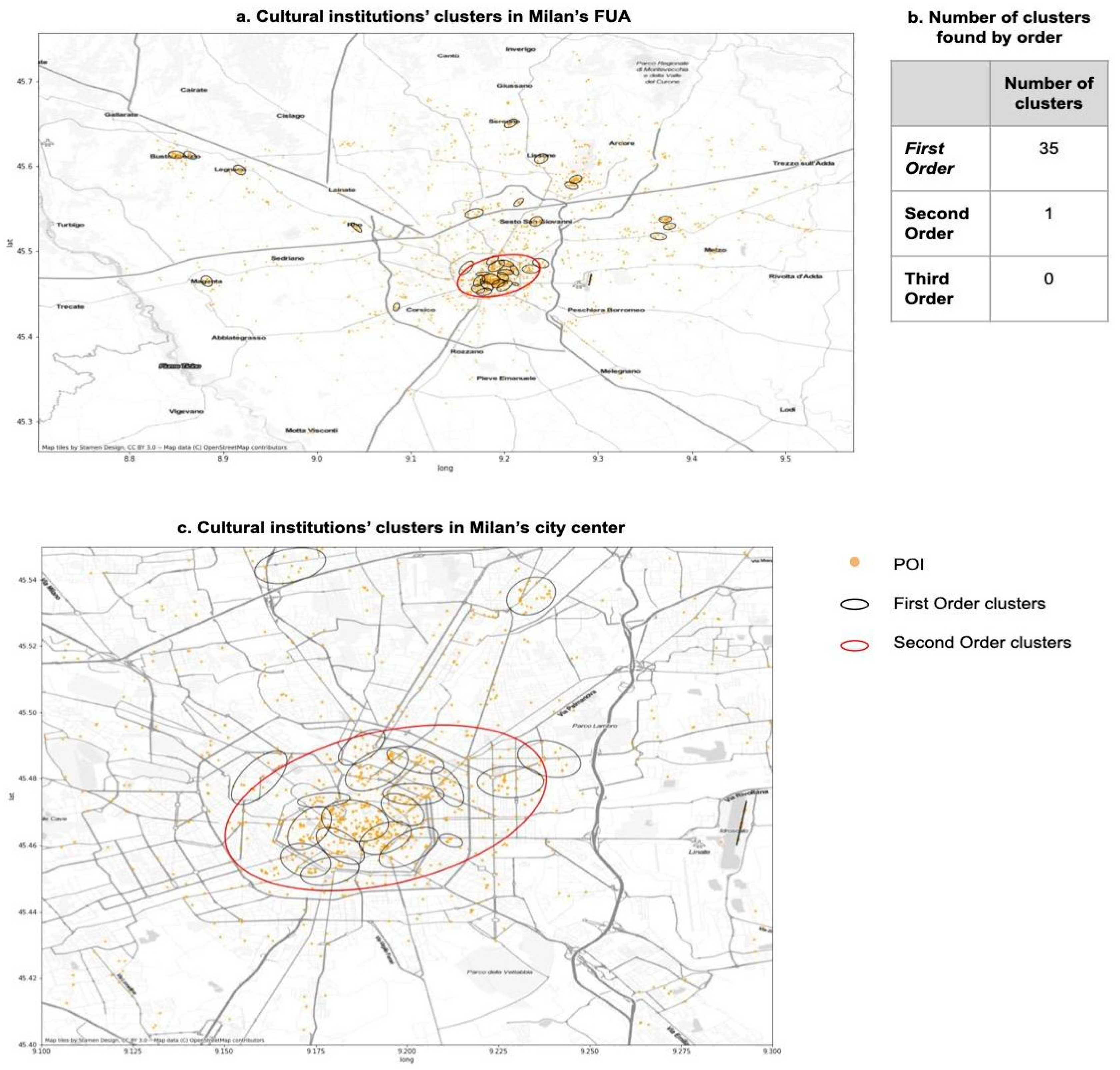
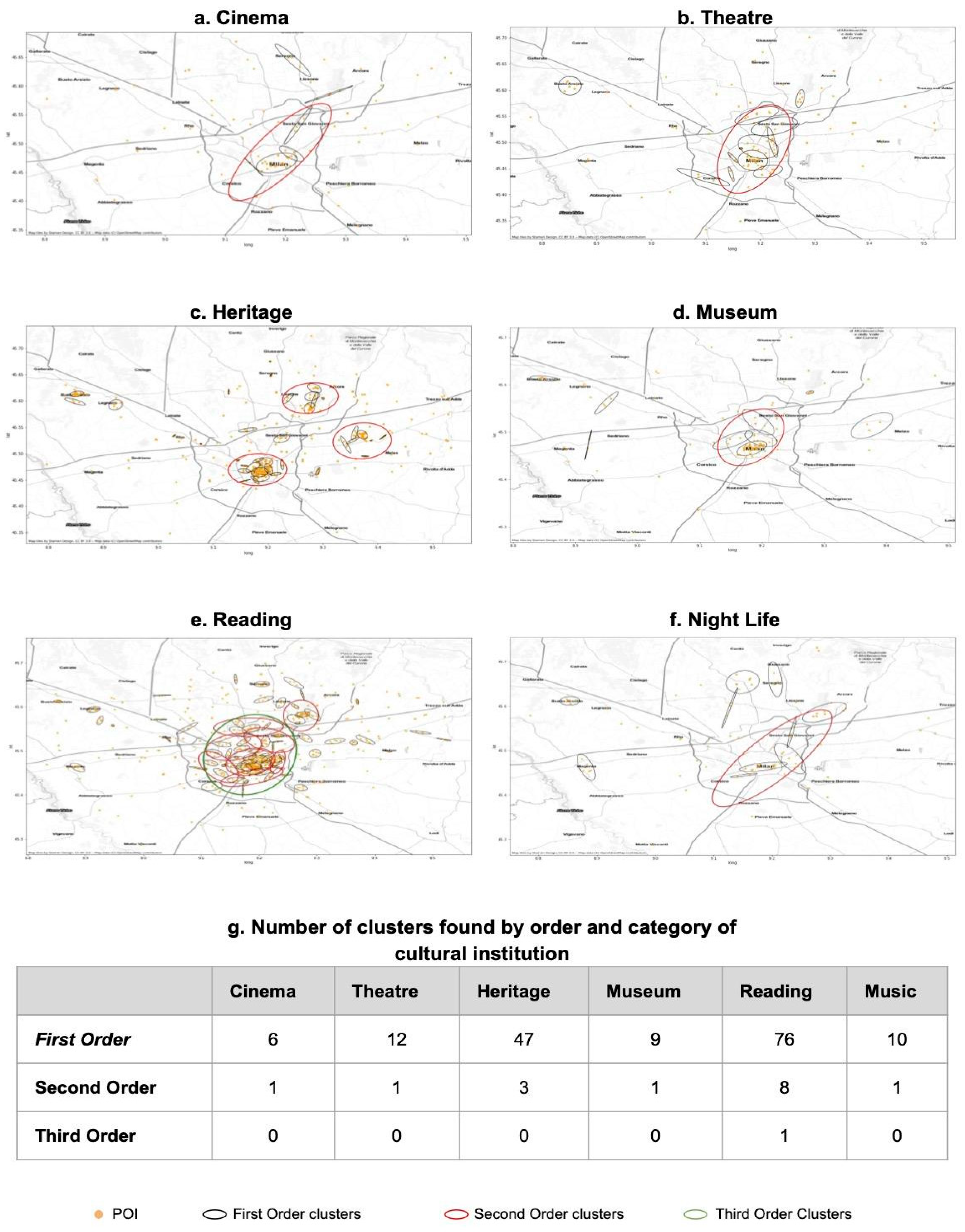
To inspect the spatial distribution of cultural amenities in our study area, we perform a cluster analysis on cultural OSM’s POIs. More specifically, from Figure A3 it can be visually inferred that first-order clusters correspond to the main urban centres in the area of analysis, while the only second-order cluster found corresponds to the centre of the municipality of Milan (Figure A3c), reflecting theories according to which culture is a mostly urban phenomenon [79] and indicating that this core–periphery pattern is replicated regardless of geographical scale. This analysis is performed using the spatial nearest neighbour hierarchical clustering algorithm—NNHC [80], already extensively used in the creative cluster literature [81], on OSM’s POIs categorised as cultural amenities according to the previously presented classification.
Figure A3. Cultural amenities’ first- and second-order clusters in Milan. (a,c) Spatial distribution of first-order (black ellipse) and second-order (red ellipse) cultural amenities throughout Milan’s functional urban area (a) and city centre (c). (b) Number of clusters found by the NNHC algorithm for each order. The NNHC algorithm defines a threshold distance and compares the threshold to the distances for all pairs of points. Only points that are closer to one or more other points than the threshold distance are selected for clustering. In addition, a minimum number of points to be included in the cluster has to be defined, and only points that fit both criteria are clustered together by the algorithm. For this analysis, the threshold distance is specified as the random nearest neighbour distance, or the expected random nearest neighbour distance for first-order nearest neighbours (for methods see [80]). The minimum number of points in a cluster is set to five cultural amenities for the aggregated analysis and two for the category-by-category one. The algorithm then conducts subsequent clustering to produce a hierarchy of clusters. The first-order clusters are themselves clustered into second-order clusters. Again, only clusters that are spatially closer than a threshold distance (calculated anew for the second level) are included.
Urbansci 09 00316 g0a3
Furthermore, spatial distribution patterns have also been investigated by sub-category of cultural amenities. The results of the NNHC algorithm show a core–periphery pattern for all categories (Figure A4). As for the results obtained over all cultural amenities mapped together, for all sub-categories, first-order clusters concentrate around the main urban centres, while second-order clusters (and third-order clusters for the reading category) concentrate throughout the municipality of Milan. At the same time, in addition to the general core–periphery spatial pattern, noticeable differences can be found when analysing sub-categories separately. Categories like theatre and cinema are almost exclusively concentrated in the municipality of Milan, with few first-order clusters located outside the ellipse of the second-order cluster found. The museum and night life sub-categories also show similar patterns, in sharp contrast to the heritage sub-category, which presents second-order clusters both over the municipality of Milan and two other smaller-scale urban areas in the province (Monza and north-east urban axis towards Gessate). The reading sub-category once again presents a core–periphery spatial pattern for first-, second-, and third-order clusters, but is more evenly distributed across the area, thanks to both its greater number of POIs and the inclusion of public libraries, which, being provided by public administrations, follow different location patterns than private amenities.
Figure A4. Cultural amenities cluster patterns by category. (af) First-, second-, and third-order clusters found by the NNHC algorithm for the categories cinema, theatre, heritage, museum, reading, and night life. (g) Number of clusters found by the NNHC algorithm for each order and each category of cultural amenities.
Urbansci 09 00316 g0a4

References

  1. Florida, R. The Rise of the Creative Class: And How It’s Transforming Work, Leisure, Community and Everyday Life. Can. Public Policy/Anal. De Polit. 2003, 29, 175–181. [Google Scholar]
  2. Markusen, A. Urban Development and the Politics of a Creative Class: Evidence from a Study of Artists. Environ. Plan. A Econ. Space 2006, 38, 1921–1940. [Google Scholar] [CrossRef]
  3. Sacco, P.L.; Crociata, A. A Conceptual Regulatory Framework for the Design and Evaluation of Complex, Participative Cultural Planning Strategies. Int. J. Urban Reg. Res. 2012, 37, 1688–1706. [Google Scholar] [CrossRef]
  4. Crociata, A.; Agovino, M.; Russo, A.; Quaglieri Dominguez, A. Creative workforce and economic development in precrisis Europe: Main trends and causality relationships. Int. Reg. Sci. Rev. 2018, 41, 448–479. [Google Scholar] [CrossRef]
  5. Lorenzen, M.; Frederiksen, L. Why do Cultural Industries Cluster? Localization, Urbanization, Products and Projects. In Creative Cities, Cultural Clusters and Local Economic Development; Edward Elgar Publishing: Cheltenham, UK, 2007. [Google Scholar] [CrossRef]
  6. Amin, A.; Thrift, N. Cultural-economy and Cities. Prog. Hum. Geogr. 2007, 31, 143–161. [Google Scholar] [CrossRef]
  7. Al, J.; Martin, R.; Sunley, P. The Rise of Cultural Economic Geography. In Economic Geography: Critical Concepts in the Social Sciences—Volume IV: The Cultural Economy; Martin, R.L., Sunley, P.J., Eds.; Routledge: London, UK, 2008; pp. 3–18. [Google Scholar]
  8. Moldavanova, A.V.; Meloche, L.; Thompson, T.L. Understanding the geography of access to cultural amenities: The case of Metropolitan Detroit. J. Urban Aff. 2021, 44, 614–639. [Google Scholar] [CrossRef]
  9. Houston, D.; Ong, P. Arts Accessibility to Major Museums and Cultural/Ethnic Institutions in Los Angeles: Can School Tours Overcome Neighborhood Disparities? Environ. Plan. A Econ. Space 2013, 45, 728–748. [Google Scholar] [CrossRef]
  10. Bertoni, A.; Dubini, P.; Monti, A. Bringing Back in the Spatial Dimension in the Assessment of Cultural and Creative Industries and Its Relationship with a City’s Sustainability: The Case of Milan. Sustainability 2021, 13, 10878. [Google Scholar] [CrossRef]
  11. Arntz, M.; Brüll, E.; Lipowski, C. Do preferences for urban amenities differ by skill? J. Econ. Geogr. 2022, 23, 541–576. [Google Scholar] [CrossRef]
  12. van Duijn, M.; Rouwendal, J. Cultural heritage and the location choice of Dutch households in a residential sorting model. J. Econ. Geogr. 2012, 13, 473–500. [Google Scholar] [CrossRef]
  13. Widdop, P.; Cutts, D. Impact of place on museum participation. Cult. Trends 2012, 21, 47–66. [Google Scholar] [CrossRef]
  14. de Graaff, T.; Boter, J.; Rouwendal, J. On Spatial Differences in the Attractiveness of Dutch Museums. Environ. Plan. A 2009, 41, 2778–2797. [Google Scholar] [CrossRef]
  15. Rodríguez-Puello, G.; Iturra, V. Does a higher cultural supply raise cultural consumption? The association between individual and city traits and cultural consumption in Chile. Ann. Reg. Sci. 2022, 72, 65–83. [Google Scholar] [CrossRef]
  16. Brook, O. Spatial equity and cultural participation: How access influences attendance at museums and galleries in London. Cult. Trends 2016, 25, 21–34. [Google Scholar] [CrossRef]
  17. Rössel, J.; Weingartner, S. Opportunities for cultural consumption: How is cultural participation in Switzerland shaped by regional cultural infrastructure? Ration. Soc. 2016, 28, 363–385. [Google Scholar] [CrossRef]
  18. Falk, M.; Katz-Gerro, T. Cultural participation in Europe: Can we identify common determinants? J. Cult. Econ. 2015, 40, 127–162. [Google Scholar] [CrossRef]
  19. Bello, P.; Garcia, D. Cultural Divergence in popular music: The increasing diversity of music consumption on Spotify across countries. Humanit. Soc. Sci. Commun. 2021, 8, 182. [Google Scholar] [CrossRef]
  20. Airoldi, M. The techno-social reproduction of taste boundaries on digital platforms: The case of music on YouTube. Poetics 2021, 89, 101563. [Google Scholar] [CrossRef]
  21. Oghina, A.; Breuss, M.; Tsagkias, M.; de Rijke, M. Predicting IMDB Movie Ratings Using Social Media. In Lecture Notes in Computer Science; Springer: Berlin/Heidelberg, Germany, 2012; pp. 503–507. [Google Scholar] [CrossRef]
  22. Bail, C.A. The cultural environment: Measuring culture with big data. Theory Soc. 2014, 43, 465–482. [Google Scholar] [CrossRef]
  23. Moreno, C.; Allam, Z.; Chabaud, D.; Gall, C.; Pratlong, F. Introducing the “15-Minute City”: Sustainability, Resilience and Place Identity in Future Post-Pandemic Cities. Smart Cities 2021, 4, 93–111. [Google Scholar] [CrossRef]
  24. Bruno, M.; Monteiro Melo, H.P.; Campanelli, B.; Loreto, V. A universal framework for inclusive 15-minute cities. Nat. Cities 2024, 1, 633–641. [Google Scholar] [CrossRef]
  25. Duranti, C.; Sacco, P.L.; Zarri, L. La domanda di cultura nelle societa’ avanzate: Premesse ad una metodologia transdisciplinare. In AICCON Working Papers 24–2005; Associazione Italiana per la Cultura della Cooperazione e del Non Profit: Forlì, Italy, 2005. [Google Scholar]
  26. Nathan, M. Creative Class Theory and Economic Performance in UK Cities. In Creative Urban Regions; IGI Global: Hershey, PA, USA, 2008; pp. 80–93. [Google Scholar] [CrossRef]
  27. Knudsen, B.; Florida, R.; Gates, G.; Stolarick, K. Urban Density, Creativity and Innovation. Available online: https://legacy.econ.tuwien.ac.at/hanappi/AgeSo/rp/Knudsen_2007.pdf (accessed on 8 May 2025).
  28. Evans, G. Participation and provision in arts & culture—Bridging the divide. Cult. Trends 2016, 25, 2–20. [Google Scholar] [CrossRef]
  29. Hill, D.; Bruno, M.; Melo, H.P.; Takeuchi, Y.; Loreto, V. Cities beyond proximity. Philos. Trans. A 2024, 382, 20240097. [Google Scholar] [CrossRef]
  30. Tahmasbi, B.; Mansourianfar, B.H.; Haghshenas, H.; Kim, I. Multimodal accessibility-based equity assessment of urban public facilities distribution. Sustain. Cities Soc. 2019, 49, 101633. [Google Scholar] [CrossRef]
  31. Taleai, M.; Sliuzas, R.; Flacke, J. An integrated framework to evaluate the equity of urban public facilities using spatial multi-criteria analysis. Cities 2014, 40, 56–69. [Google Scholar] [CrossRef]
  32. Omer, I. Evaluating accessibility using house-level data: A spatial equity perspective. Comput. Environ. Urban Syst. 2006, 30, 254–274. [Google Scholar] [CrossRef]
  33. Bertoni, A.; Dubini, P.; Monti, A. Participatory Event Platforms in the Urban Context: The Importance of Stakeholders’ Meaning of “Participation”. In Cultural Initiatives for Sustainable Development. Contributions to Management Science; Demartini, P., Marchegiani, L., Marchiori, M., Schiuma, G., Eds.; Springer: Cham, Switzerland, 2021. [Google Scholar] [CrossRef]
  34. Currid, E.; Williams, S. The geography of buzz: Art, culture and the social milieu in Los Angeles and New York. J. Econ. Geogr. 2009, 10, 423–451. [Google Scholar] [CrossRef]
  35. Grodach, C. Mapping the arts: Industry concentrations, distribution, and change in the US, 1980–2010. Int. J. Cult. Policy 2014, 22, 353–375. [Google Scholar] [CrossRef]
  36. Grodach, C.; Currid-Halkett, E.; Foster, N.; Murdoch, J., III. The location patterns of artistic clusters: A metro- and neighborhood-level analysis. Urban Stud. 2014, 51, 2822–2843. [Google Scholar] [CrossRef]
  37. Brook, O.; Boyle, P.; Flowerdew, R. Geographic Analysis of Cultural Consumption. In Spatial and Social Disparities; Springer: Dordrecht, The Netherlands, 2010; pp. 67–82. [Google Scholar] [CrossRef]
  38. Foster, N.; Grodach, C.; Murdoch, J., III. Neighborhood Diversity, Economic Health, and The Role of the Arts. J. Urban Aff. 2016, 38, 623–642. [Google Scholar] [CrossRef]
  39. Galster, G. The mechanism (s) of neighbourhood effects: Theory, evidence, and policy implications. In Neighbourhood Effects Research: New Perspectives; van Ham, M., Manley, D., Bailey, N., Simpson, L., Maclennan, D., Eds.; Springer: Dordrecht, The Netherlands, 2011; pp. 23–56. [Google Scholar]
  40. Palshikar, G.K. Fuzzy region connection calculus in finite discrete space domains. Appl. Soft Comput. 2004, 4, 13–23. [Google Scholar] [CrossRef]
  41. Launhardt, W. Mathematische Begrflndung der Volkswirtschaflslehre; Springer: Leipzig, Germany, 1885. [Google Scholar]
  42. Weber, A. Ueber den Standort der Industrien; JCB Mohr: Tiibingen, Germany, 1909. [Google Scholar]
  43. Von Thunen, A. Der Isolierte Staat in Beziehung Auflandwirtschafl yon NationalOkonomie; Walter de Gruyter GmbH & Co KG: Hamburg, Germany, 1826. [Google Scholar]
  44. Bourdieu, P. The Forms of Capital. In Handbook of Theory and Research for the Sociology of Education; Richardson, J.G., Ed.; Greenwood Press: New York, NY, USA, 1983; pp. 241–258. [Google Scholar]
  45. Belfiore, E. Art as a means of alleviating social exclusion: Does it really work? A critique of instrumental cultural policies and social impact studies in the UK. Int. J. Cult. Policy 2002, 8, 91–106. [Google Scholar] [CrossRef]
  46. Coffee, K. Cultural inclusion, exclusion and the formative roles of museums. Mus. Manag. Curatorship 2008, 23, 261–279. [Google Scholar] [CrossRef]
  47. Kavanagh, G. Museums and the First World War: A Social History; A&C Black: London, UK, 2014. [Google Scholar]
  48. Sandell, R. Museums as agents of social inclusion. Mus. Manag. Curatorship 1998, 17, 401–418. [Google Scholar] [CrossRef]
  49. Katz-Gerro, T. Cultural consumption research: Review of methodology, theory, and consequence. Int. Rev. Sociol. 2004, 14, 11–29. [Google Scholar] [CrossRef]
  50. Lizardo, O.; Skiles, S. Musical taste and patterns of symbolic exclusion in the United States 1993–2012: Generational dynamics of differentiation and continuity. Poetics 2015, 53, 9–21. [Google Scholar] [CrossRef]
  51. Turel, O.; Serenko, A.; Bontis, N. User acceptance of hedonic digital artifacts: A theory of consumption values perspective. Inf. Manag. 2010, 47, 53–59. [Google Scholar] [CrossRef]
  52. Ferraro, A.; Cerciello, M.; Agovino, M.; Garofalo, A. The role of cultural consumption in reducing social exclusion: Empirical evidence from Italy in a spatial framework. Econ. Politica 2019, 36, 139–166. [Google Scholar] [CrossRef]
  53. Crociata, A.; Agovino, M.; Sacco, P.L. Recycling waste: Does culture matter? J. Behav. Exp. Econ. 2015, 55, 40–47. [Google Scholar] [CrossRef]
  54. Quaglione, D.; Cassetta, E.; Crociata, A.; Sarra, A. Exploring additional determinants of energy-saving behaviour: The influence of individuals’ participation in cultural activities. Energy Policy 2017, 108, 503–511. [Google Scholar] [CrossRef]
  55. Schläpfer, M.; Dong, L.; O’Keeffe, K.; Santi, P.; Szell, M.; Salat, H.; Anklesaria, S.; Vazifeh, M.; Ratti, C.; West, G.B. The universal visitation law of human mobility. Nature 2021, 593, 522–527. [Google Scholar] [CrossRef]
  56. Biazzo, I.; Monechi, B.; Loreto, V. General scores for accessibility and inequality measures in urban areas. R. Soc. Open Sci. 2019, 6, 190979. [Google Scholar] [CrossRef]
  57. Alessandretti, L.; Aslak, U.; Lehmann, S. The scales of human mobility. Nature 2020, 587, 402–407. [Google Scholar] [CrossRef]
  58. Dong, X.; Morales, A.; Jahani, E.; Moro, E.; Lepri, B.; Bozkaya, B.; Sarraute, C.; Bar-Yam, Y.; Pentland, A. Segregated interactions in urban and online space. EPJ Data Sci. 2020, 9, 20. [Google Scholar] [CrossRef]
  59. Melo, H.P.; Henriques, J.; Carvalho, R.; Verma, T.; Da Cruz, J.P.; Araújo, N.A.M. Heterogeneous impact of a lockdown on inter-municipality mobility. Phys. Rev. Res. 2021, 3, 013032. [Google Scholar] [CrossRef]
  60. Arsanjani, J.; Zipf, A.; Mooney, P.; Helbich, M. OpenStreetMap in GIScience: Experiences, Research, and Applications; Springer: Cham, Switzerland, 2015. [Google Scholar]
  61. Hariharan, R.; Toyama, K. Project Lachesis: Parsing and modeling location histories. In International Conference on Geographic Information Science; Max, E., Freksa, F., Harvey, M., Eds.; Springer: Berlin/Heidelberg, Germany, 2004; pp. 106–124. [Google Scholar]
  62. OECD. Functional Urban Areas: Italy. 2022. Available online: https://www.oecd.org/en/data/datasets/oecd-definition-of-cities-and-functional-urban-areas.html (accessed on 8 May 2025).
  63. mapMI|Ask. (n.d.). Available online: https://green.unibocconi.eu/research/research-areas/arts-societies-knowledge-economie-ask/art-histories-heritage-and-cultural (accessed on 8 May 2025).
  64. d’Ovidio, M.; Cossu, A. Culture is reclaiming the creative city: The case of Macao in Milan, Italy. City Cult. Soc. 2017, 8, 7–12. [Google Scholar] [CrossRef]
  65. Sacco, P.; Tavano Blessi, G. The Social Viability of Culture-led Urban Transformation Processes: Evidence from the Bicocca District, Milan. Urban Stud. 2009, 46, 1115–1135. [Google Scholar] [CrossRef]
  66. Biferale, L.; Brandano, M.G.; Crociata, A. The spatial dimensions of cultural consumption: How distance influences consumption levels in a spatial setting. J. Cult. Econ. 2024, 48, 499–525. [Google Scholar] [CrossRef]
  67. Ritzer, G. Enchanting a Disenchanted World: Revolutionizing the Means of Consumption; Pine Forge Press: Thousand Oaks, CA, USA, 1999. [Google Scholar]
  68. Meyer, H.-D. Taste Formation in Pluralistic Societies. Int. Sociol. 2000, 15, 33–56. [Google Scholar] [CrossRef]
  69. Zhao, S.; Elesh, D. The Second Digital Divide: Unequal Access to Social Capital in the Online World. Int. Rev. Mod. Sociol. 2007, 33, 171–192. [Google Scholar]
  70. Katz-Gerro, T. Highbrow cultural consumption and class distinction in Italy, Israel, West Germany, Sweden, and the United States. Soc. Forces 2002, 81, 207–229. [Google Scholar] [CrossRef]
  71. Wright, D. Mediating production and consumption: Cultural capital and ‘cultural workers’. Br. J. Sociol. 2005, 56, 105–121. [Google Scholar] [CrossRef] [PubMed]
  72. Prieur, A.; Savage, M. Emerging forms of cultural capital. Eur. Soc. 2013, 15, 246–267. [Google Scholar] [CrossRef]
  73. Oakley, K.; O’Brien, D. Learning to labour unequally: Understanding the relationship between cultural production, cultural consumption and inequality. Soc. Identities 2016, 22, 471–486. [Google Scholar] [CrossRef]
  74. Dobilas, M. LOWESS Regression in Python: How to Discover Clear Patterns in Your Data? Towardsdatascience.com. 2020. Available online: https://towardsdatascience.com/lowess-regression-in-python-how-to-discover-clear-patterns-in-your-data-f26e523d7a35 (accessed on 8 May 2025).
  75. Pinto, C.M.A.; Mendes Lopes, A.; Machado, J.A.T. A review of power laws in real life phenomena. Commun. Nonlinear Sci. Numer. Simul. 2012, 17, 3558–3578. [Google Scholar] [CrossRef]
  76. Biferale, L.; Comunian, R.; Dent, T. “Where are culture and creativity in your city?” Chrono-urbanism and the importance of pluralism in defining and understanding cultural opportunities in cities. Cities 2025, 166, 106221. [Google Scholar] [CrossRef]
  77. Domenech, R.; Lazzeretti, L.; Oliver, J.; Molina, B.; Ruiz, B. Creative clusters in Europe: A microdata approach. In ERSA Conference Papers ersa11p471, Proceedings of the 51st Congress of the European Regional Science Association, Barcelona, Spain, 30 August–3 September 2011; European Regional Science Association: Ottignies, Belgium, 2011. [Google Scholar]
  78. DISCE. Measuring Creative Economies: A Critical Review of CCI. No. D2.1. 2022. Available online: https://disce.eu/wp-content/uploads/2022/07/DISCE-D2.1-updated.pdf (accessed on 27 November 2022).
  79. Pratt, A.C. Creative cities: The cultural industries and the creative class. Geogr. Ann. Ser. B Hum. Geogr. 2008, 90, 107–117. [Google Scholar] [CrossRef]
  80. NIJ. Crimestat III: A Spatial Statistics Program for the Analysis of Crime Incident Locations; The National Institute of Justice: Washington, DC, USA, 2004.
  81. Lazzeretti, L.; Boix, R.; y Capone, F. Why do creative industries cluster? An analysis of the determinants of clustering of creative industries. In Creative Industries and Innovation in Europe; Lazzeretti, L., Ed.; Routledge: London, UK, 2011. [Google Scholar]
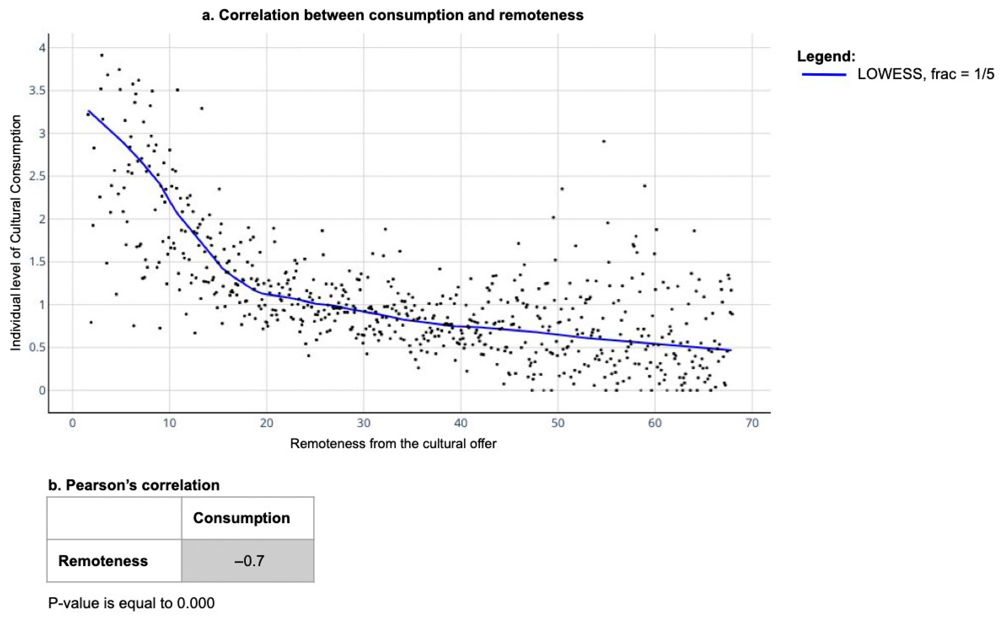
Figure 1. Correlation of the level of consumption with remoteness from cultural amenities. (a) Scatter plot of C i against R i . (b) Pearson’s correlation of C i and R i . The scatter plot shows the locally weighted scatterplot smoothing (LOWESS) algorithm, a supervised learning regression algorithm used for regression analysis where data attributes do not allow linear regression models to produce a good fit [74]. Note: to increase the readability of the data visualisations and to reduce the noise of the data at the users’ level, remoteness values (x) have been rounded (one decimal place), and y variables have been averaged over each rounded x. All correlations hold true for non-rounded and non-averaged values as well.
Urbansci 09 00316 g001
Figure 2. Spatial distribution of cultural consumption and remoteness from cultural amenities. (a) Spatial distribution of per-hexagon average remoteness from cultural amenities ( R h ) over the entire study area. The colour gradient reflects quartiles of variable distribution: Q1 = lowest remoteness—higher proximity (lowest 25%), Q4 = highest remoteness—lower proximity (top 25%). The black border represents the extension of Milan’s municipality, and red borders indicate the extension of the six most populated municipalities in Milan’s metropolitan area (Busto Arsizio, Sesto San Giovanni, Cinisello Balsamo, Vigevano, Legnano, Rho). (b) The same map as (a) but zoomed in over the area of Milan’s municipality. (c) Spatial distribution of per-hexagon average values of individual level of consumption ( C I ). The colour gradient reflects quartiles of variable distribution: Q1 = least consumption (lowest 25%), Q4 = highest consumption (top 25%). The black and red borders, as in (a), represent the extension of municipal borders in the study area. (d) The same map as (c) but zoomed in over the area of Milan’s municipality. (e) Moran’s spatial autocorrelation index for the two variables mapped.
Urbansci 09 00316 g002
Figure 3. Correlation of consumption level with remoteness from cultural amenities at the individual level. (a) Scatter plot of C i (in a log scale) against R i for the four categories of individuals, including the Pearson’s correlation coefficients. The four categories are: PRONE individuals in the top-right quadrant, AVERSE individuals in the bottom-left quadrant, CONSUMERS in the top-left quadrant, and NON-CONSUMERS in the bottom-right quadrant. (b) Scatter plot of C i (in a log scale) against R i for individuals with consumption levels lower than the sample’s mean (NON-CONSUMERS + AVERSE individuals) in the bottom half of the graph and scatter plot of C i (in a log scale) against R i for individuals with consumption levels higher than the sample’s mean (CONSUMERS + PRONE individuals) in the top half of the graph, including the Pearson’s correlation coefficients.
Urbansci 09 00316 g003
Figure 4. Power law distribution. (a) Plot of the log-log transformation of C i against R i for all users. (b) Scatter plot of C i against R i for all users together with the plot of the power law distribution fitted to the data. (c) The values of R^2, the intercept, and the coefficient of the linear regression model plotted over the log-log transformed data for different intervals of the data range ( R i ). Obtaining similar results for different data ranges validates the power law assumption.
Urbansci 09 00316 g004
Figure 5. Relative composition of each hexagon by category of individuals. (a) Spatial distribution of the per-hexagon relative composition of individuals with consumption levels higher than the sample’s mean (CONSUMERS + PRONE). The black border represents the extension of Milan’s municipality, and red borders indicate the extension of the six most populated municipalities in Milan’s metropolitan area (Busto Arsizio, Sesto San Giovanni, Cinisello Balsamo, Vigevano, Legnano, Rho). (b) Spatial distribution of the per-hexagon relative composition of individuals with consumption levels lower than the sample’s mean (NON-CONSUMERS + AVERSE). Black and red borders, as in (a), represent the extension of municipal borders in the study area. (c) Moran’s spatial autocorrelation index for all the variables mapped.
Urbansci 09 00316 g005
Table 1. Proposed classification of cultural amenities.
CategoryOSM Tags
HeritageHistoric building; monument; ruins; castle; attraction
MuseumMuseum, art gallery, zoo, planetarium, aquarium
ReadingLibrary
CinemaCinema
TheatreTheatre
Night LifeConcert hall, night club, dance hall
Table 2. Dataset structure.
CategoryPOIsUnique UsersTrips
Total POIs50,396330,92916,082,194
Total Cultural POIs1070190,149489,130
Cinema8648,55358,481
Theatre11237,86444,605
Night Life8626,96631,548
Reading368107,136160,114
Museum13054,47974,710
Heritage28877,821119,672
Disclaimer/Publisher’s Note: The statements, opinions and data contained in all publications are solely those of the individual author(s) and contributor(s) and not of MDPI and/or the editor(s). MDPI and/or the editor(s) disclaim responsibility for any injury to people or property resulting from any ideas, methods, instructions or products referred to in the content.