Accident Impact Prediction Based on a Deep Convolutional and Recurrent Neural Network Model

Abstract

Traffic accidents pose a significant threat to public safety, resulting in numerous fatalities, injuries, and a substantial economic burden each year. The development of predictive models capable of the real-time forecasting of post-accident impact using readily available data can play a crucial role in preventing adverse outcomes and enhancing overall safety. However, existing accident predictive models encounter two main challenges: first, a reliance on either costly or non-real-time data, and second, the absence of a comprehensive metric to measure post-accident impact accurately. To address these limitations, this study proposes a deep neural network model known as the cascade model. It leverages readily available real-world data from Los Angeles County to predict post-accident impacts. The model consists of two components: Long Short-Term Memory (LSTM) and a Convolutional Neural Network (CNN). The LSTM model captures temporal patterns, while the CNN extracts patterns from the sparse accident dataset. Furthermore, an external traffic congestion dataset is incorporated to derive a new feature called the “accident impact” factor, which quantifies the influence of an accident on surrounding traffic flow. Extensive experiments were conducted to demonstrate the effectiveness of the proposed hybrid machine learning method in predicting the post-accident impact compared to state-of-the-art baselines. The results reveal a higher precision in predicting minimal impacts (i.e., cases with no reported accidents) and a higher recall in predicting more significant impacts (i.e., cases with reported accidents).

1. Introduction

Traffic crashes are a major public safety concern, leading to significant fatalities, injuries, and economic burdens annually. In 2020, the fatality rate on American roads saw a staggering 24% increase compared to 2019, the largest year-over-year rise since 1924, according to the National Safety Council (NSC). Understanding the causes and impacts of traffic accidents is crucial for evaluating highway safety and addressing negative consequences, including high fatality and injury rates, traffic congestion, carbon emissions, and related incidents. Despite the ample existing literature, the development of accurate and efficient accident prediction models remains a challenging and fascinating research area.

Over recent decades, a wide range of predictive and computational methods have been proposed to predict traffic accidents and their impacts [1]. These models progressed from linear to nonlinear models and from traditional predictive regression models [2,3,4] to today’s most common data analytic and machine learning algorithms [5,6,7]. A majority of the studies treat the problem as a standard binary classification task [8,9], with the output being a categorical event (accident or non-accident), with no information on the post-accident consequences. Furthermore, existing studies that investigated post-accident impacts mostly failed to provide a compelling way to define and measure the “impact”, which is a significant challenge. The most commonly used metric to measure and illustrate the impact of accidents on traffic flow is “duration”. However, to our understanding, this metric is not ideal because it can be influenced by various environmental factors, including the type of road and accessibility conditions. For example, if a road has accessibility issues, it may take longer to clear an accident scene, resulting in a longer duration. Furthermore, the datasets typically utilized for these studies are not publicly available and cannot be employed in real-time projects.

In recent years, hybrid neural networks that integrate multiple architectures have attracted increasing attention for their ability to model complex, real-world phenomena. Marcillo et al. [10] review learning-based models for traffic accident prediction and highlight deep learning methods—particularly LSTM and CNN—as the most effective, due to their strengths in handling temporal and spatial data, respectively. This review also emphasizes the need for high-quality, heterogeneous data and effective strategies to address data imbalance and high dimensionality. Motivated by recent findings, we propose a cascaded LSTM-CNN architecture tailored to the spatiotemporal nature of traffic data. LSTM captures long-term temporal dependencies, while CNN efficiently extracts local spatial and short-term temporal patterns [11]. This hybrid model addresses key challenges such as data heterogeneity and high dimensionality, aiming to enhance predictive accuracy. Furthermore, we introduce a novel metric to quantify accident impact on surrounding traffic flow, bridging a gap in prior work that focused primarily on accident occurrence rather than its broader effects.

LSTM and CNN models are sequentially combined in terms of a “cascade” model. We specifically chose these two models because of their ability to handle temporal dependencies effectively. Furthermore, their combination offers a stronger capability to distinguish between accident and non-accident events, especially in imbalanced datasets, compared to using each model individually. Our model performs better in discriminating high-impact accidents. It achieves this by first distinguishing between accident and non-accident events and subsequently predicting the post-accident impact of the accident events. In more detail, the cascade model utilizes a sequence of the last T time intervals (e.g., a two-hour interval) within each specific region (e.g., a zone specified by a square of size 5 km × 5 km on map) to predict the probability of an accident and its post-impact in that region for the next time interval (i.e., $T+1$).

This study utilizes four complementary, easy-to-obtain, real-world datasets to build and evaluate the proposed prediction framework. The first dataset provides real-world accident data across the United States; it contains location, time, duration, distance, and severity. The second dataset offers detailed weather information such as weather conditions, wind chill, humidity, temperature, etc. The third dataset contains spatial attributes for each district (e.g., the number of traffic lights, stop signs, and highway junctions). The fourth dataset is a traffic congestion dataset that provides real-world congestion data across the United States. The congestion dataset is also used to develop a novel target feature, gamma, representing an accident’s impact on its surrounding area. We propose a data-driven solution to define gamma as a function of three accident-impact-related features, duration, distance, and severity. Generally, non-accident intervals are far more prevalent in the real world compared to accident intervals (since accidents are relatively infrequent events). Therefore, working with such an imbalanced dataset poses challenges for model development and evaluation. To address this issue, we employ a random under-sampling method to mitigate the imbalanced nature of the dataset. Using these settings and through extensive experiments and evaluations, we demonstrate the effectiveness of the cascade model in predicting post-accident impact compared to state-of-the-art models that were evaluated using the same datasets. It is worth noting that the datasets used in this research are generally easy to obtain, regarding how they have been collected (more details can be found in [12]) and the replicability of the data collection processes for other regions.

The main contributions of this paper are summarized as follows:

• A real-world setup for post-accident impact prediction: This paper proposes an effective setup to use easy-to-obtain, real-world data resources (i.e., datasets on accident events, congestion incidents, weather data, and spatial information) to estimate accident impact on the surrounding area shortly after an accident occurs. Also, this framework employs a data augmentation approach to obtain accurate feature vectors from heterogeneous data sources.
• A data-driven label refinement process: This study illustrates a novel feature to demonstrate post-accident impact on its surrounding traffic flow. This feature combines three factors, namely “severity”, “duration”, and “distance”, to create a compelling feature that we refer to as gamma in this work.
• A cascade model for accident impact prediction: This paper proposes a cascade model to employ the power of LSTM and CNN to efficiently predict the post-accident impacts in two stages. First, it distinguishes between accident and non-accident events, then it predicts the intensity of impact for accident events.

To provide a clear overview of our study design, Figure 1 presents the research workflow. The process begins with the collection and integration of four real-world datasets, followed by data preprocessing, feature engineering, and the construction of a novel post-accident impact label. The processed data is then passed through a two-stage cascade model: first, an LSTM predicts the likelihood of an accident; if an accident is detected, a CNN subsequently classifies its impact severity. The workflow concludes with model evaluation and comparison, followed by discussion of key insights and practical implications.

The remainder of the article is organized as follows. Section 2 provides an overview of related studies, followed by a description of data in Section 3. Section 4 describes our accident labelling approach, and then the cascade model is presented in Section 5. Section 6 illustrates experimentation design and results, and Section 7 concludes the paper by discussing essential findings and recommendations for future studies.

2. Related Work

Traffic accident analysis and prediction have been the focus of extensive research over recent decades. Broadly, prior work in this field falls into two main categories: accident risk prediction, which seeks to estimate the likelihood or frequency of accidents occurring, and accident impact prediction, which aims to assess the consequences and disruptions caused by accidents. In the following subsections, we review key studies and advances within each of these categories, highlighting major methodological trends and identifying remaining gaps addressed by our work.

2.1. Accident Risk Prediction

Research on accident risk prediction has evolved through the application of diverse methodologies and data sources, generally aiming to (1) estimate accident rates in a region or (2) classify the likelihood of accident occurrence in specific locations or intervals [13,14].

Early works in this area focused on statistical and classical machine learning models. Regression-based techniques have been widely used for accident rate prediction, often incorporating fundamental attributes such as traffic volume, road type, and historical incident records [15,16,17]. In the context of accident detection and classification, binary classifiers such as SVMs [18] and k-nearest neighbor or Bayesian models [19] have been effectively employed. Many studies enhanced these predictions through advanced feature selection methods, such as the use of decision trees for variable filtering [18] or frequent pattern trees for uncovering important data patterns [19].

As the volume and diversity of available data have increased, a key trend has been the integration of temporal and spatial dependencies into predictive models. Several studies leveraged time-series analysis and recurrent structures to capture temporal patterns in accident data [20,21,22]. Others extended this paradigm by considering spatial correlations across road networks or urban zones, with graph-based and deep learning models offering notable improvements in cases where location and neighborhood effects are significant [16,23,24].

With the rise of deep learning, more recent works increasingly employ neural architectures to accommodate high-dimensional, heterogeneous, and sequential traffic data. Deep neural networks, including stacked autoencoders and hybrid LSTM-CNN designs, have consistently demonstrated higher accuracy and robustness for accident risk prediction than traditional methods [11,24,25,26]. Notably, these approaches often integrate multi-source data (e.g., traffic flow, weather, road characteristics) to enrich their feature spaces. For example, Moosavi et al. [27] developed a hybrid deep model for large-scale detection; Chen et al. [17] applied a stacked denoising autoencoder on GPS-derived accident severity; and Ren et al. [15] used an LSTM to predict traffic accident counts, though with a limited feature set. Expanding the diversity of input data, Chen et al. [28] and Li et al. [11] exploited novel sources such as vehicle license plate recognition and detailed signal timing.

In addition, methodological advances such as self-organizing maps have been utilized to improve model calibration and fine-tune neural networks for spatially extensive road sections, as shown by Kaffash et al. [29], who achieved high predictive accuracy over thousands of roadway points. A summary of the above studies can be found in

Table 1. A summary of previous works on accident risk prediction.

Study	Input Features	Predicted Output	Model	Best Modeling Results
Moosavi et al. [27]	1. Weather conditions 2. Time of day 3. Location 4. Road features	Accident risk on different road segments	DNN with recurrent, fully connected and embedding components)	F1 score = 0.59 for accident class F1 score = 0.89 for non-accident class
Li et al. [11]	1. Traffic flow characteristics 2. Signal timing 3. Weather condition	Real-time crash risk	LSTM-CNN	False alarm rate = 0.132 AUC = 0.932
Parsa et al. [30]	1. Traffic 2. Network 3. Demographic 4. Land use 5. Weather feature	Occurrence of accidents	eXtreme Gradient Boosting (XGBoost)	Accuracy = close to 100%, Detection rate = varies between 70% and 83%, false alarm rate is less than 0.4%
Yu and Abdel-Aty [18]	1. Crash data 2. Real-time traffic data	Crash occurrence	SVM with RBF kernel	AUC = 0.74 for all crash type, AUC = 0.80 for Multi-vehicle crashes, AUC = 0.75 for Single-vehicle crashes (evaluated on 30% of the whole dataset)
Ozbayoglu et al. [9]	1. Average velocity 2. Occupancy 3. The capacity difference between time t and t + 1 4. Weekday/weekend 5. Rush hour	Crash occurrence	Nearest neighbor (NN), Regression tree (RT), feedforward neural network (FNN),	Accuracy = 95.12 for NN Accuracy = 97.59 for RT Accuracy = 99.79 for FNN

. Taken together, the literature reveals clear progress from regression and classical machine learning toward deep learning models that systematically exploit spatial and temporal information as well as a richer array of features. However, most prior work remains focused on the occurrence or frequency of accidents, rather than the downstream effects such incidents have on traffic and congestion. Moreover, although deep models have improved predictive performance, limited attention has been paid to developing coherent, actionable metrics for post-accident impact or to integrating contextual features in a way that supports interpretability and generalization.

2.2. Accident Impact Prediction

A substantial body of work has focused on analyzing and predicting the post-accident impact on surrounding areas. The majority of these studies characterize “impact” using accident duration, severity, or clearance time as core indicators, and employ a range of predictive models. Traditional approaches typically use regression techniques to estimate the duration and magnitude of post-accident disruptions, considering factors such as traffic flow, road geometry, and incident details [31,32,33,34]. As modeling techniques advanced, neural networks and other machine learning algorithms were applied to capture complex, nonlinear effects among input variables [5,35,36].

A number of recent studies have refined these paradigms by expanding data inputs and comparing multiple modeling strategies. For example, Zhang et al. [2] combined loop detector and police data to define the total impact as the sum of accident duration and clearance time and compared the predictive power of multiple linear regression to artificial neural networks. Yu et al. [37] explored a range of binary features (weather, time of day, presence of disabled vehicles, and peak hour) for predicting incident duration on freeways, finding that ANNs performed better for long-duration incidents, while SVMs were more accurate for shorter-duration cases. Ensemble methods have also been used: Ma et al. [38] reported superior interpretability and prediction accuracy for gradient boosting decision trees in forecasting clearance time compared to methods such as SVMs, neural networks, and random forests.

While most prior work defines impact in terms of duration or severity, a minority of studies have attempted to forecast downstream traffic metrics. Yu et al. [39] stands out by modeling post-accident traffic flow, although their analysis was limited to a single route. Lin et al. [40] investigated the prediction of different post-accident traffic condition states using SVM, neural network, and random forest models and incorporated incremental learning by updating predictions as new data became available during an event. Ensemble approaches continue to gain traction, with recent work demonstrating the effectiveness of CatBoost ensemble algorithms for predicting the impact range of traffic accidents and addressing common issues such as overfitting and generalization in accident impact models [41]. More recently, Ekanem [42] employed logistic regression, random forest, and XGBoost to predict accident severity in Victoria, Australia, identifying temporal features as significant predictors; however, the models faced challenges in accurately predicting rare but severe (fatal) cases, with the authors recommending resampling strategies as a remedy. A summary of the above studies is provided in

Table 2. A summary of previous works on accident impact prediction.

Study	Input Features	Predicted Output	Model	Best Modeling Results
Zhang et al. [2]	1. Temporal 2. Spatial 3. Environmental 4. Traffic 5. Accident details	Total duration and clearance time	Multiple linear regression and ANN	MAPE = 27.1% for total duration, MAPE = 49.8% for clearance time
Ekanem [42]	1. Accident time, 2. Accident date, 3. Day of the week, 4. Road surface condition, 5. Accident type, etc.	Accident severity class: Fatal, Serious injury, Minor injury, Property damage only	Logistic Regression, Random Forest, XGBoost	Logistic Regression achieved 100% recall for minor injuries, but all models struggled with fatal cases%
Ma et al. [38]	1. Accident details 2. Temporal 3. Geographical 4. Environmental 5. Traffic 6. Operational	Incident clearance time	Gradient boosting decision trees (GBDT)	MAPE = 16% for clearance time less than 15 min and MAPE = 33% for clearance time more than 15 min
Rose Yu et al. [39]	1. Accident type 2. Downstream post mile 3. Affected traffic direction 4. Traffic speed	The delay corresponding to the accident	Mixture Deep LSTM	MAPE = 0.97
Yu and Abdel-Aty [18]	1. Crash data 2. Real-time traffic data	Crash occurrence	SVM	AUC = 0.74 for SVM with RBF for all crash type
Lin and Li [40]	1. Accident details 2. Traffic details 3. Environmental 4. Air quality 5. Geographical	TAPI (derived from post-accident congestion level and its duration)	NN, SVM, RF	MAPE = 5.5–53.8%
Wang et al. [35]	1. Vehicle type 2. Location 3. Time of day 4. Report mechanism	Vehicle breakdown duration	fuzzy logic (FL) and ANN	RMSE = 24 for FL model RMSE = 19.5 for ANN mode V1 RMSE = 24.1 for ANN mode V2

.

In summary, while prior research has advanced modeling techniques for accident impact prediction, most studies use narrow definitions of impact—typically limited to duration or severity—and focus on small geographic areas. Few works combine multiple impact dimensions or apply composite metrics at scale. Our study addresses these gaps by introducing a novel, composite impact metric (integrating duration, severity, and blockage distance) and evaluating it across the large and diverse region of Los Angeles County. We rely on openly available data sources—such as BingMaps and MapQuest for traffic, Weather Underground for weather (examples: Microsoft BingMaps (https://www.microsoft.com/en-us/maps/ (accessed on 3 June 2025)), MapQuest (https://www.mapquest.com/ (accessed on 3 June 2025)), Weather Underground (https://www.wunderground.com/history (accessed on 3 June 2025)), and OpenStreetMap (https://www.openstreetmap.org (accessed on 3 June 2025))) and OpenStreetMap for spatial features—which facilitates replicability and broader application. More details on dataset collection and preparation can be found in [12].

3. Dataset

This section describes all datasets used to build our accident impact prediction framework. In addition to describing original datasets, the processes of data cleaning, transformation, and augmentation are also described. Lastly, we briefly study accident duration distribution and compare it with findings presented by other researchers. It is worth noting that accident duration refers to the time-span required to clear the impact of an accident, and we believe that it is highly correlated with accident impact. Hence, further studying it would help to derive valuable insights when building the predictive model.

3.1. Data Sources

The data sources and study areas are related to Los Angeles County, the most accident-prone county in the United states (see https://www.iihs.org/topics/fatality-statistics/detail/state-by-state (accessed on 3 June 2025) for more details). Four datasets are used to deliberate all factors involved in the aftermath of accident: the accident dataset, congestion dataset, point of interest (poi) dataset, and weather dataset. The following sub-sections describe these datasets in detail.

3.1.1. Accident Dataset

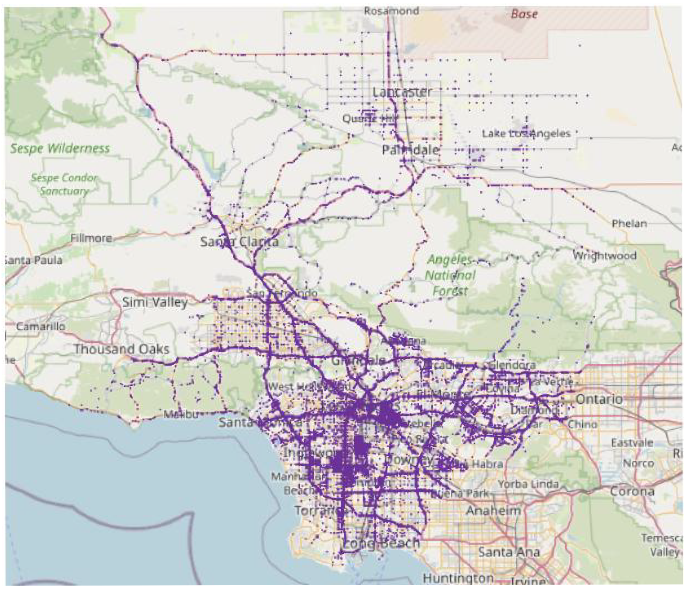
This study adopts the US-Accident dataset, a large-scale traffic accident dataset compiling data collected from all over the United States [43] between 2016 and 2020. This dataset contains accident events collected from two sources, MapQuest Traffic and Microsoft BingMaps, and it covers 49 states of the United States. A total of 73,553 accident records were extracted that cover four years from August 2016 to December 2020. Figure 2 shows the dispersion of accident location in the area of study that covers both freeway and urban arterial roads. Features of reported accidents are listed in

Table 3. Accident dataset features.

Category	Features
Geographical features	Start latitude, Start longitude, End latitude, End longitude, Distance, Street, Number, Airport code, City, Country, State, Zip code, Side, Amenity, Bump, Crossing, Give way, Junction, No-exit, Railway, Roundabout, Station, Stop, Traffic Calming, Traffic Signal, Turning Loop
Temporal features	Start time, End time, Time zone, Sunrise Sunset, Civil Twilight, Nautical Twilight, Astronomical Twilight
Other	ID, Severity, TMC

. The reader can find a detailed description of features at smoosavi.org/datasets/us_accidents (accessed on 3 June 2025).

3.1.2. Congestion Dataset

Traffic congestion events are essential to predict and also to measure accident impact. The congestion dataset provided in [12] that includes such incidents over the same period and location is considered as the accident data. This dataset includes over 600,000 congestion events, collected between 2016 and 2020, where each event was recorded when traffic speed was slower than typical traffic speed. In addition to the basic details (such as the time and location of a congestion case), the dataset also offers other valuable details such as delay and average speed (the latter is in the form of natural language description of an event reported by a human agent). “Severe delays of 22 min on San Diego Fwy Northbound in LA. Average speed ten mph.” is an example of the description attribute, which offers details such as the exact “delay” and “speed” of the congestion. One can easily extract such details from the free-form text via regular expression patterns. In this work, we use congestion data for accident impact labeling, which is thoroughly discussed in Section 4.

3.1.3. POI Dataset

As previous studies have shown, road features have a significant impact on determining the possibility of accidents [27]. As a result, road-network features must be considered when predicting and measuring the impact of accidents. This study utilizes a POI dataset taken from OpenStreetMap (OSM) that provides the geographical features of each location, such as the number of railroads, speed bumps, traffic signals, and pedestrian crossings.

3.1.4. Weather Condition Dataset

Numerous studies have shown the significant impact of weather condition on accident prediction [44,45,46]. While airport stations may be located some distance from urban centers, they offer reliable and regionally representative weather data. This research considers the weather data that had been collected from weather stations located in four airports in Los Angeles area (i.e., Los Angeles International Airport (LAX), Hollywood Burbank Airport (BUR), Van Nuys Airport (VNY), and Whiteman Airport (KWHP)). The four airports listed above offer hourly weather characteristics for the period of study. Each record includes the following features: airport, date, hour, temperature, wind chill, humidity, pressure, visibility, wind speed, wind direction, precipitation, and weather conditions. The last two are categorical features, and all their possible values are shown in

Table 4. Details of categorical weather features.

Features	Unique Values
Weather Conditions	’Mostly Cloudy’, ’Scattered Clouds’, ’Partly Cloudy’, ’Clear’, ’Light Rain’, ’Overcast’, ’Heavy Rain’, ’Rain’, ’Haze’, ’Patches of Fog’, ’Fog’, ’Shallow Fog’, ’Thunderstorm’, ’Light Drizzle’, ’Thunderstorms and Rain’, ’Cloudy’, ’Fair’, ’Mist’, ’Mostly Cloudy / Windy’, ’Fair / Windy’, ’Partly Cloudy / Windy’, ’Light Rain with Thunder’
Wind Directions	’E’, ’W’, ’CALM’, ’S’, ’N’, ’SE’, ’NNE’, ’NNW’, ’SSE’, ’ESE’, ’NE’, ’NW’, ’WSW’, ’ENE’, ’SW’, ’SSW’, ’WNW’

.

3.2. Data Quality Assurance

Although the datasets used in this study are publicly available and widely adopted in transportation research, we conducted a set of quality checks to ensure that the input data was reliable and suitable for downstream modeling. This included reviewing all features for semantic consistency, confirming that the categorical fields used well-defined value sets, and inspecting numerical attributes for plausible ranges.

We also assessed data completeness and addressed missing values and anomalies where appropriate. For instance, missing entries in the weather dataset were handled using a k-nearest neighbors imputation approach, and outliers in numerical features were managed using standard range-based filtering. Details of these methods are described in the next section. Duplicate records were removed, and low-frequency spatial zones were excluded to reduce sparsity and improve model stability.

These quality assurance steps provided a cleaner and more coherent input space, allowing the model to learn from consistent and interpretable patterns without being affected by noise or structural inconsistencies.

3.3. Preprocessing and Preparation

This section describes the required steps to preprocess different sources of data that are used in this work. Further, the proposal to build input data by combining different sources to be used for modeling is described. In terms of preprocessing, we can elaborate the following steps:

• Remove duplicated records: Since the accident data is collected from two potentially overlapping sources, some accidents might be reported twice. Therefore, we first process the input accident data to remove duplicated cases.
• Fill missing values using K-Nearest Neighbors imputation: The weather data suffers from missing values for some of features (e.g., sunrise_sunset). Based on two nearest neighbors, we impute missing values with the mean (for numerical features) or mode (for categorical features). We use time and location to determine distance when finding neighbors. This approach leverages the smooth variation in weather data across space and time. For cases with higher missingness, more advanced imputation methods could be explored in future work.
• Treat outliers: For a numerical feature f, if $f_i>{\mu }_f+3{\sigma }_f$ or $f_i<{\mu }_f-3{\sigma }_f$, then we replace it with ${\mu }_f+3{\sigma }_f$ or ${\mu }_f-3{\sigma }_f$, respectively. Here, ${\mu }_f$ and ${\sigma }_f$ are the mean and standard deviation of feature f, respectively, calculated on all weather records. This three-sigma range is a standard statistical method that effectively removes extreme outlier values while preserving the vast majority of valid data.
• Omit redundant features: We remove those features that satisfy either of the following conditions: (1) correlated features based on Pearson correlation; (2) categorical features with more than 90% data frequency on a specific value.
• Discretize data: After data cleaning, both accident and congestion data are first discretized in space and time. The temporal resolution is 2 h intervals and the spatial resolution is set to 5 km × 5 km squares in uniform grids.

Overall, 26 input features are chosen based on domain knowledge, literature precedence, and preliminary correlation analysis, and refined by removing highly correlated or low-variance features as discussed above during preprocessing.

A vector like $l(s.t)\in R^m$ is used to represent the input data at time t in region s, applied for accident impact prediction. This vector represents the input for the predictive task, and later we describe labeling. In this way, we convert raw data to $l(s.t)\in R^{26}$, which consists of 5 categories of features that include 26 different features obtained from raw datasets.

Table 5. Selected features after preprocessing and preparation.

Feature Category	Feature
Temporal	Day of Week, Part of Day (day/night), Sunrise/Sunset
Weather	Weather Condition
Accident	Severity, Accident Count, Duration, Distance
Congestion	Congestion Count, Congestion Delay
Spatial	Geohash Code, latitude, longitude, Amenity, Bump, Crossing, Give way, Junction, No-exit, Railway, Roundabout, Station, Stop, Traffic Calming, Traffic Signal, Turning Loop

describes details of features used to create an input vector. In addition, due to the rarity of accident events and data sparsity, we drop those zones for which the total number of recorded accidents is less than a certain threshold $\alpha$ during the two years. By setting $\alpha =75$, which means dropping zones with less than 75 reported accidents in 2 years (i.e., the accidents which were reported in less than 0.8% of time intervals), the ratio of time intervals with at least one reported accident (also known as accident intervals) to all intervals increases by 4.8%. The value of $\alpha =75$ was set based on exploratory data analysis to ensure each selected region contained a sufficient number of accident events for robust model training, while avoiding excessive data sparsity. Lower thresholds led to too many regions with insufficient data for reliable prediction, while higher thresholds resulted in too few regions and reduced spatial diversity. Thus, $\alpha =75$ provides a balance between data adequacy per zone and representative spatial coverage of the study area. In Section 5.2 an under-sampling method is discussed to balance the ratio of accident to non-accident intervals to a larger extent.

3.4. Data Augmentation

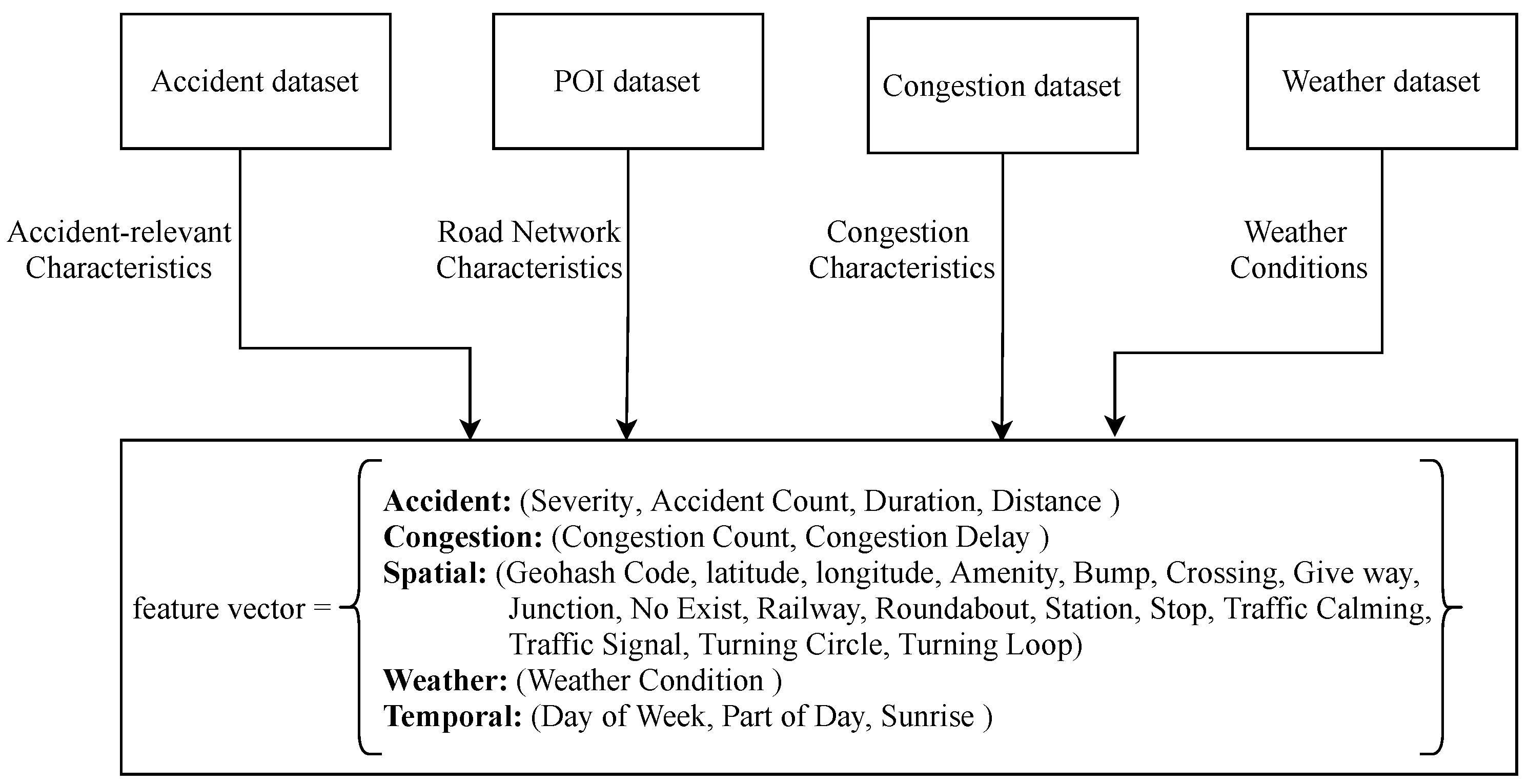
The initial accident dataset includes a variety of features. However, we only use highly accident-relevant features, and further augment the data with additional features described in Section 3.1 to create the input feature vector. Road-network characteristics of regions are added to differentiate between various types of urban and suburban regions, congestion-related information is added to empower the model in finding latent patterns between accident and congestion events, and weather data collected from the nearest airport based on accident’s occurrence time and location is used to further help the model by encoding weather condition data. Figure 3 summarizes how the input feature vector is built in this study.

To define a proper accident prediction task over geographical areas during different time intervals, it is required to build input data for accident-free time intervals. The data are discretized in space and time in order to build these non-accident (or accident-free) intervals (described in Section 3.3). When no accident is reported for an interval, accident-related features (i.e., severity, accident count, duration and distance) are set to zero, and the remaining features (i.e., geographical, temporal, surrounding congestion and weather conditions) are filled in accordingly using available resources.

3.5. Accident Duration Distribution

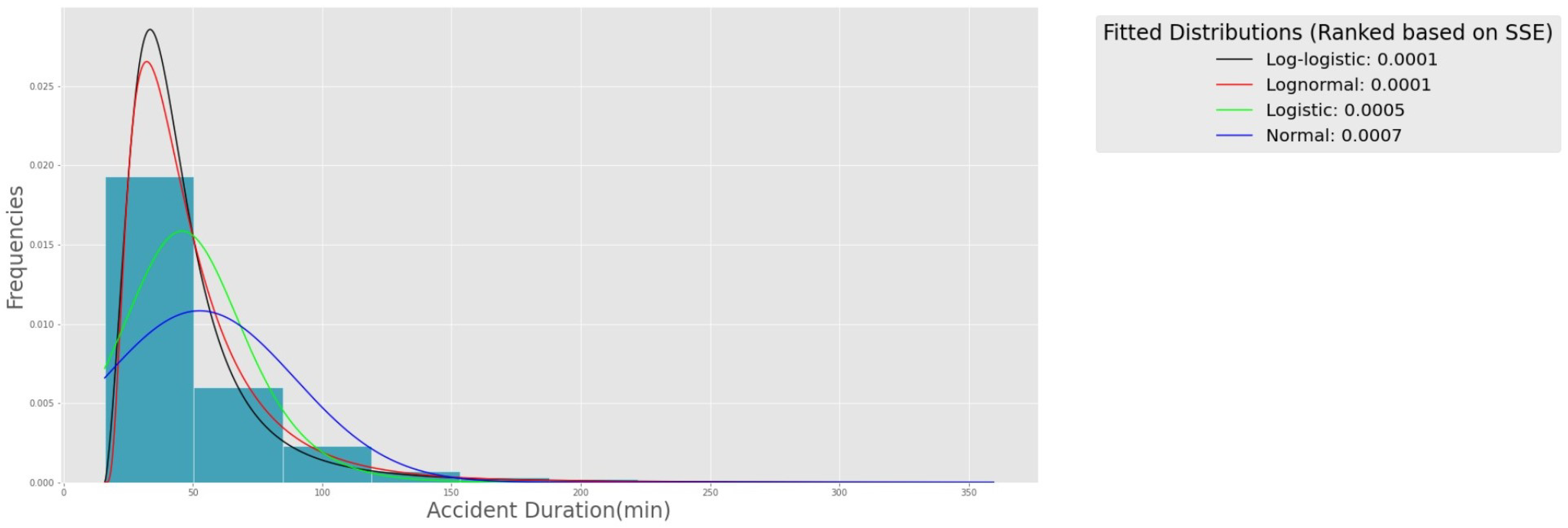
Accident duration is an essential factor to determine impact. Thus, it is worth studying this factor to see how its distribution in our dataset is aligned with datasets that were used in the literature. Previous studies found that a log-normal distribution can best model accident duration [2,47,48].

This section investigates this phenomenon using the input data and compares the research findings with [2]. First, we divide the duration dataset into K classes based on Doane’s formula [47]:

$$K={log}_{2}n+{log}_2\left(1+{\displaystyle \frac{\left|g1\right|}{{\sigma }_{g1}}}\right)$$

(1)

where n stands for the total number of observations and $g1$ refers to the estimated third-moment-skewness of the observations:

$${\sigma }_{g_1}=\sqrt{{\displaystyle \frac{6(n-2)}{(n+1)(n+3)}}}$$

(2)

Class $C_i,i\in 1,2,\cdots ,K$ is specified by its upper bound $(min\left(D\right)+i\times {\displaystyle \frac{max\left(D\right)-min\left(D\right)}{K}})$ and lower bound $(min\left(D\right)+(i-1)\times {\displaystyle \frac{max\left(D\right)-min\left(D\right)}{K}})$, where D is the accident duration. Then, the frequency of each class is calculated and summation of the squared estimate of errors between the frequency of each class and the probability density function of fitted distribution is calculated.

The sum of the squared estimate of errors (SSE) calculated for four selected distributions is shown in Figure 4. Log-normal and log-logistic distributions have the lowest SSE and therefore describe accident duration data the best. This is aligned with findings reported by Zhang et al. [2]. They used the AIC (Akaike Information Criterion) and the BIC (Bayesian Information Criterion). They found log-normal and log-logistic distributions to be the first and the second best-fitted distributions, respectively.

4. Label Development of Post-Accident Impact

The previous section discussed data sources, pre-processing, and augmentation steps. However, we have not yet described “accident impact” in terms of a quantitative feature or attribute. To the best of our knowledge, there is no exact parameter to show the impact of the accident on its surrounding traffic flow in the real world. There are a number of studies addressing the effect of traffic congestion on accidents [49,50,51], while the effect of traffic accidents on traffic congestion has been rarely studied [23,52]. Of these few studies, some researches used accident duration as an indicator for an accident’s impact, while some others studied the effects of speed changes in surrounding traffic flow as an indicator. We believe that none of these approaches are comprehensive and genuine enough to describe how traffic flow would be affected by the occurrence of an accident.

In this study, we propose a novel “accident impact” feature based on the delay caused by accidents. This is achieved by finding a function $\mathcal{F}$ from the congestion dataset to estimate delay based on the accident dataset. In the following, a detailed explanation of the process can be found.

4.1. Accident Impact: A Derived Factor

There are three attributes in our dataset that can be used to determine “impact”:

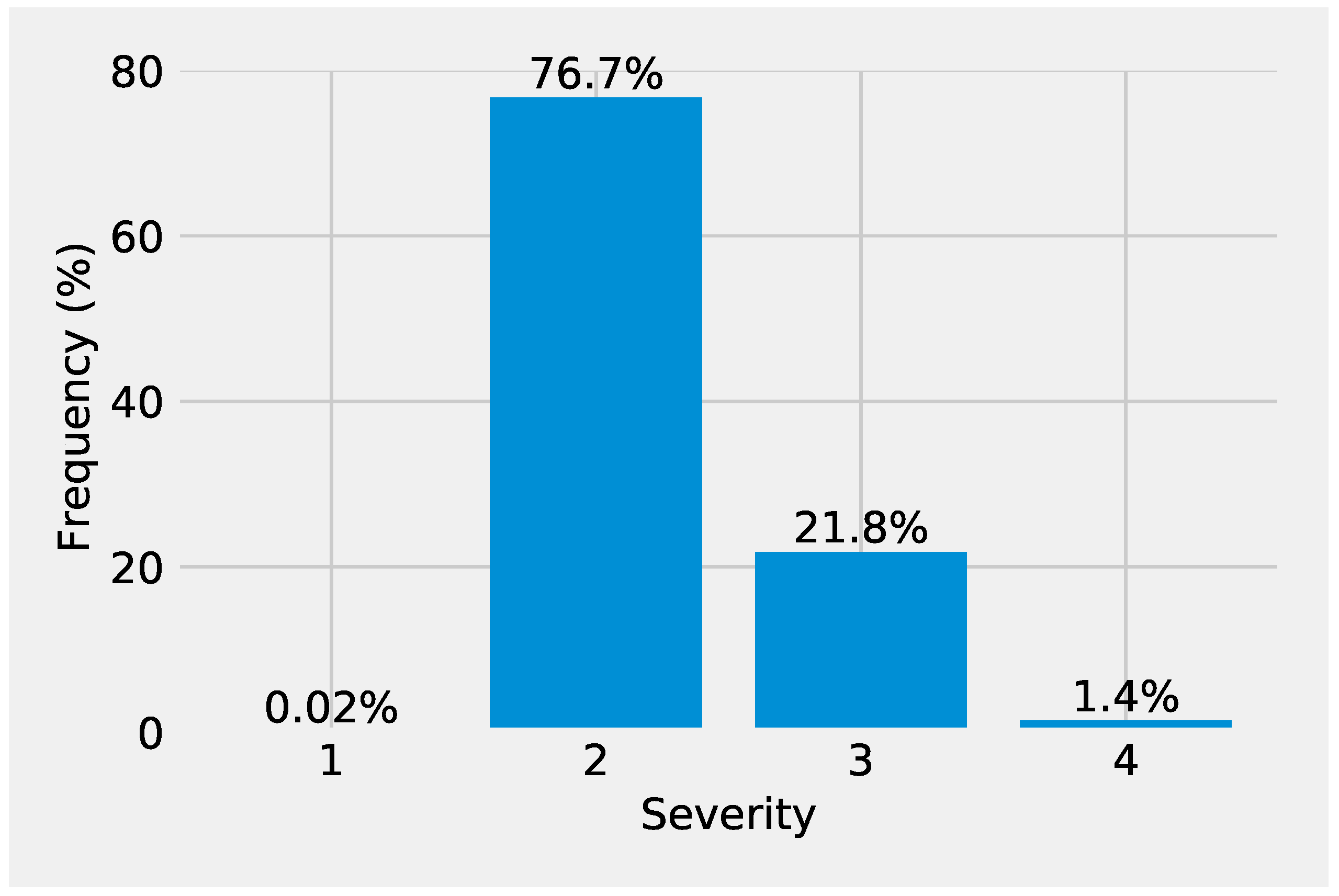
• Severity: This is a categorical attribute that shows severity in terms of delay in free-flow traffic due to accidents. It is defined by the original data providers based on real-time traffic conditions and reports, where 1 indicates minimal disruption and 4 indicates significant traffic delays. Although it seems to be a highly relevant feature, it suffers from skewness when looking at its distribution (see Figure 5), and is a coarse-grained factor (i.e., it is represented by just a few categorical values).
• Duration: The duration of a traffic accident shows the period from when the accident was first reported until its impact had been cleared from the road network. In this sense, the duration can be considered as another factor to determine impact. Please note that a long duration does not necessarily indicate a significant impact, as it could be related to the type of location and accessibility concerns. However, generally speaking, duration is positively correlated with impact.
• Distance: Distance shows the length of road affected by an accident. Similar to duration, a long distance does positively correlate with higher impact. However, a high-impact accident may not necessarily result in impacting a long extent of road.

All three attributes can, to some extent, represent the impact of an accident. However, each alone may not suffice to define the impact primarily. Thus, we propose building a model that can estimate accident impact given these features as input.

4.2. Delay as a Proxy for Impact

To estimate accident impact, a function $\mathcal{F}$ is defined that maps the three input features to a target value $\gamma$, which we refer it as “impact”:

$$\gamma =\mathcal{F}(\mathit{Severity},\mathit{Duration},\mathit{Distance})$$

Now, the question is, how do we find $\mathcal{F}$? While there is no straight-forward approach to estimate $\mathcal{F}$ based on accident data, if we choose to fit it on congestion data (see Section 3.1.2), we can use some extra signals from the input to estimate the desired function. For congestion events, our data offers a human-reported description of incidents that includes “delay” (in minutes) with respect to typical traffic flow (see

Table 6. Examples of congestion events and features used to build function F.

Event ID	Description	Severity	Duration (Minute)	Distance (Mile)
1	Delays increasing and delays of nine minutes on Colorado Blvd Westbound in LA. Average speed five mph.	Slow	49.6	2.42
2	Delays of three minutes on Harbor Fwy Northbound between I-10 and US-101. Average speed 20 mph.	Moderate	43.5	3.18
3	Delays of eight minutes on Verdugo Rd Southbound between Verdugo Rd and Shasta Cir. Average speed five mph.	Slow	41.6	0.55
4	Delays of two minutes on I-5 I-10 Northbound between Exits 132 132A Calzona St and Exit 135A 4th St. Average speed 20 mph.	Fast	41.6	2.26

for some examples). To the best of our knowledge, the “description” is generated by traffic officials in a systematic way, and therefore it is reliable and accurate. Supposing that the impact in the congestion domain is represented by delay (which is a fair assumption given our definition of impact and what delay represents), we can fit $\mathcal{F}$ on congestion data using delay as the target. Please note that “delay” is only available in the congestion dataset, and here the goal is to derive it for accidents and use it as the target value.

After fitting $\mathcal{F}$ on congestion events, it is used to estimate impact (represented by $\gamma$) for accidents. It is worth noting that, according to our data, congestion and accident events share the same nature, given their attributes and the sources that have been used to collect them. Thus, fitting a function like $\mathcal{F}$ on one and applying it on another is a reasonable design choice.

4.3. Estimating Delay

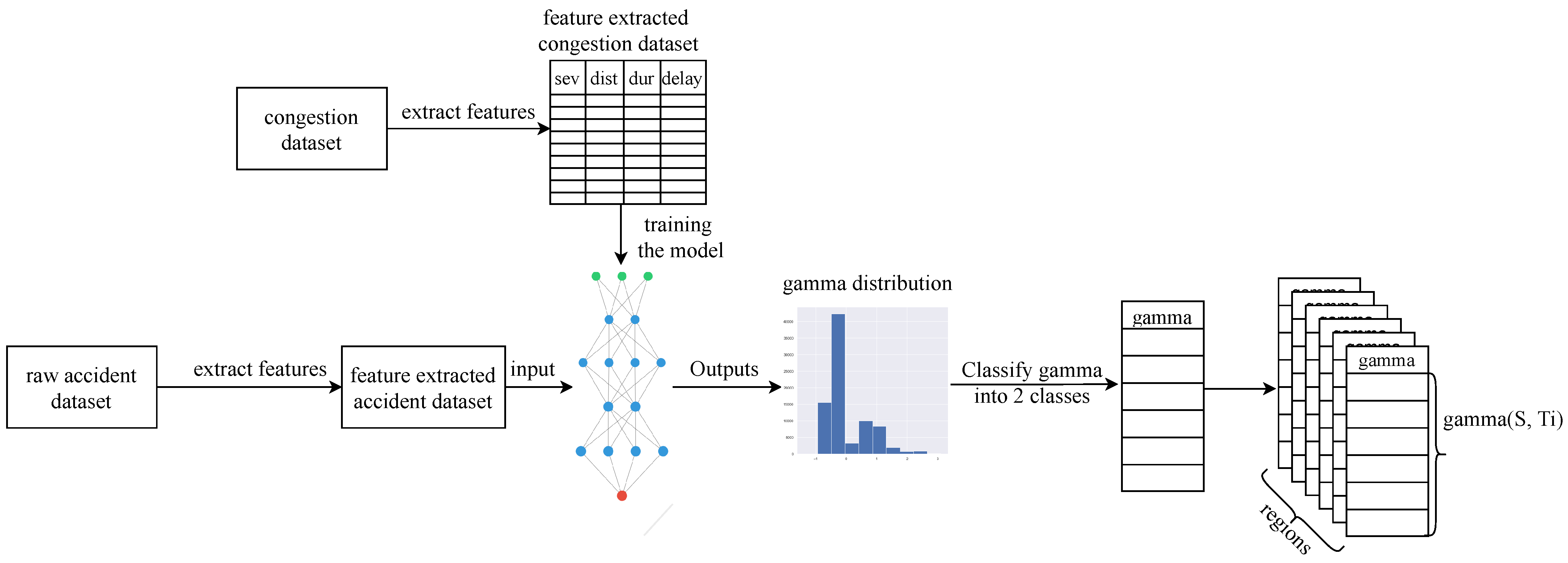
The reported delays associated with congestion events are extracted from their description and used as our $\gamma$ variables (i.e., target values). The aim is to find $\mathcal{F}$ by fitting different functions on data and select the best one with lower Mean Squared Error (MSE) and Mean Absolute Error (MAE) values. The overall process is described in Figure 6. Two models are used to estimate $\mathcal{F}$:

• Linear regression (LR) model: Given our input features, a linear model seems a natural choice to estimate $\gamma$. So, we use a linear regression model for this purpose.
• Artificial Neural Network (ANN): To examine the impact of non-linearity to estimate $\gamma$, we also used a multi-layer perceptron network with four layers, each with three neurons, and a single neuron in the last layer. We used the Adam optimizer [53] with a learning rate of $0.0008$ and trained the model for 200 epochs.

To train these models, in total, 48,109 congestion records collected between June 2018 and August 2019 are used. The algorithm considers $85\%$ of the data for the training and $15\%$ for evaluation.

Table 7. Result of using ANN and LR models to predict delay (as a proxy for impact) on congestion data.

Model	ANN	LR
MSE	0.141	0.153
MAE	0.239	0.255

shows the results of different models to predict delay using the three input features. Based on these results, the non-linear model (i.e., ANN) is selected to estimate the delay (or $\gamma$).

In the following, we discuss why it is reasonable to use the function fitted on congestion events and apply it to accident events. First, in our data, there is a resemblance between accidents and congestion events, given their attributes and the sources used to collect them. Second, we define the reported delay associated with congestion as gamma, so with similar inputs from another type of traffic event, the output would be of the nature of delay, which in our opinion is a better indicator of the impact of a traffic accident in comparison to duration or speed changes.

After obtaining $\gamma$ values for accident events, we categorize them into two different classes to show the impact of accidents using more detectable labels: “medium severity” and “high severity”. A value of $\gamma$ lower than the median is labeled as “medium severity”, and a $\gamma$ higher than the median is labeled as “high severity”. Although one could pick a finer-grained categorization of $\gamma$ values (e.g., three or four classes), through the empirical studies, we found that the choice of two categories best represents our data.

Please note that $\gamma$, as a real value, is not a proper target feature for accident impact prediction since there are numerous contributing factors determining the exact value of accident delay (in seconds or minutes) which cannot be collected in advance. Therefore, the aim is to classify $\gamma$ into two classes (i.e., “medium severity” and “high severity” ) to deal with this natural drawback of the accident impact prediction task.

4.4. Scope of Predicted Accident Impact

It is important to clarify that the focus of this study is on predicting the traffic-related consequences of accidents, not their human or medical outcomes. Specifically, the goal of our model is to estimate the post-accident impact on traffic flow, such as increased congestion or travel delay, using a derived indicator called ($\gamma$). This indicator is estimated using congestion-related features such as delay, severity, and affected distance, as outlined in Section 4.2. Our framework does not attempt to predict health outcomes such as injuries, fatalities, or emergency response outcomes, as this would require detailed individual-level incident and medical data, which are not available in the datasets used. Instead, our focus is on developing a real-time, data-driven method to quantify and forecast traffic disruption caused by accidents—a perspective aligned with applications in traffic management and urban mobility planning. Future extensions of this work could consider incorporating the prediction of health outcomes if appropriate and reliable data become available.

5. Accident Impact Prediction Methodology

This section presents our modeling approach for predicting the impact of traffic accidents using spatiotemporal urban data. The nature of this task poses two key challenges. First, the input data is high-dimensional and heterogeneous, combining weather, congestion, road structure, and historical accident records across both space and time. Second, the learning objective involves classifying both the occurrence and the severity of accidents in the presence of significant class imbalance. Addressing these challenges requires a model that can learn both sequential dependencies and spatial structure from complex urban data [16].

To this end, we propose a two-stage cascade model that leverages the complementary strengths of LSTM and CNN architectures. The first stage uses an LSTM network to detect the likelihood of an accident in the next interval. LSTMs are well-suited for this purpose, as they have been shown to effectively capture long-term temporal dependencies in traffic and transportation systems [54,55,56]. By learning from recent sequences of temporal features, this model identifies patterns that precede accident occurrences.

The second stage of the cascade uses a CNN to predict the impact severity of accident events identified in the first stage. CNNs are commonly used for spatial pattern recognition and have demonstrated strong performance in traffic applications where features are arranged over grids or maps [11,57,58]. In our setup, spatial and short-term temporal features such as congestion delay, road layout, and local conditions are encoded into structured input, allowing the CNN to learn discriminative patterns associated with different impact levels.

This modular design allows each component to specialize in a subtask: temporal event detection or spatial impact classification. It also improves interpretability, reduces overfitting risk by narrowing the prediction scope of each stage, and helps to mitigate the challenges associated with imbalanced data.

In the remainder of this section, we first introduce key background concepts related to LSTM and CNN architectures, then describe how input data is structured and labeled, and finally detail the model architecture and training procedure.

5.1. Basic Concepts

5.1.1. Long Short-Term Memory

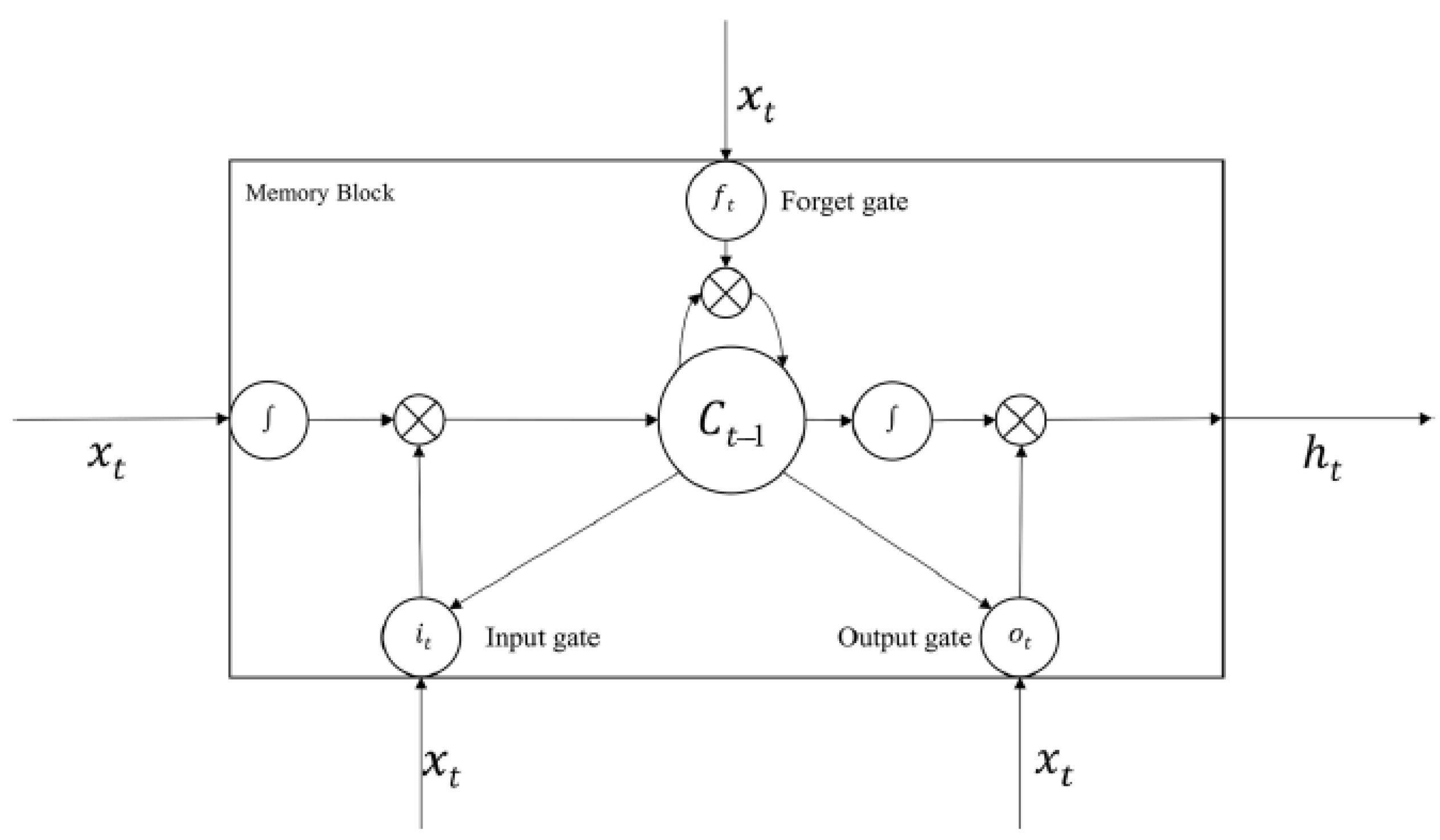
The LSTM model proposed by Hochreiter and Schmidhuber [59] is a variant of the recurrent neural network (RNN) model. It builds a specialized memory storage unit during training through a time backpropagation algorithm. It is designed to avoid the vanishing gradient issue in the original RNN. The key to LSTMs is the cell state, which allows information to flow along with the network. LSTM can remove or add information to the cell state, carefully regulated by structures called gates, including the input gate, forget gate, and output gate. The structure of a LSTM unit at each time step is shown in Figure 7. The LSTM generates a mapping from an input sequence vector $X=(X_1,X_t,\dots ,X_N)$ to an output probability vector by calculating the network units’ activation using the following equations (t shows iteration index):

$$\begin{array}{cc}\hfill i_t& ={\sigma }_g(W_{ix}{X}_t+W_{ih}{h}_{t-1}+W_{ic}{c}_{t-1}+b_i)\hfill \end{array}$$

(3)

$$\begin{array}{cc}\hfill f_t& ={\sigma }_g(W_{fx}{X}_t+W_{hf}{h}_{t-1}+W_{cf}{c}_{t-1}+b_f)\hfill \end{array}$$

(4)

$$\begin{array}{cc}\hfill o_t& ={\sigma }_g(W_{ox}{X}_t+W_{oh}{h}_{t-1}+W_{oc}{c}_t+b_o)\hfill \end{array}$$

(5)

$$\begin{array}{cc}\hfill c_t& =f_t\odot c_{t-1}+i_t\odot {\sigma }_c(W_{cx}{X}_t+W_{ch}{h}_{t-1}+b_c)\hfill \end{array}$$

(6)

$$\begin{array}{cc}\hfill h_t& =o_t\odot {\sigma }_g\left(c_t\right)\hfill \end{array}$$

(7)

$$\begin{array}{cc}\hfill y_t& =W_{yh}{h}_{t-1}+b_y\hfill \end{array}$$

(8)

where X is the input vector. W and b are weight matrices and bias vector parameters, respectively, that need to be learned during training. ${\sigma }_c$ and ${\sigma }_g$ are sigmoid and hyperbolic tangent function, respectively, and ⊙ indicates the element-wise product of the vectors. The forget gate $f_t$ controls the extent to which the previous step memory cell should be forgotten, the input gate $i_t$ determines how much update each unit, and the output gate $o_t$ controls the exposure of the internal memory state. The model can learn how to represent information over several time steps as the values of gating variables vary for each time step.

5.1.2. Convolutional Neural Network

CNN is a multi-layer neural network which includes two important components for feature extraction: convolution and pooling layers. Figure 8 shows the overall structure of the convolution neural network. Its basic structure includes two special neuronal layers. The first one is the convolution layer; the input of each neuron in this layer is locally connected to the previous layer, and this layer seeks to extract local features. The second layer is the pooling layer, used to find the local sensitivity and perform secondary feature extraction [60]. The number of convolutions and pooled layers depends on the specific problem definition and objectives. Firstly, the model uses a convolutional layer to generate latent features based on the input (Figure 9a). Then, a sub-sampling layer is used on top of the convolutional output to extract more high-level features for the classification or recognition task (Figure 9b).

5.2. Model Input and Output

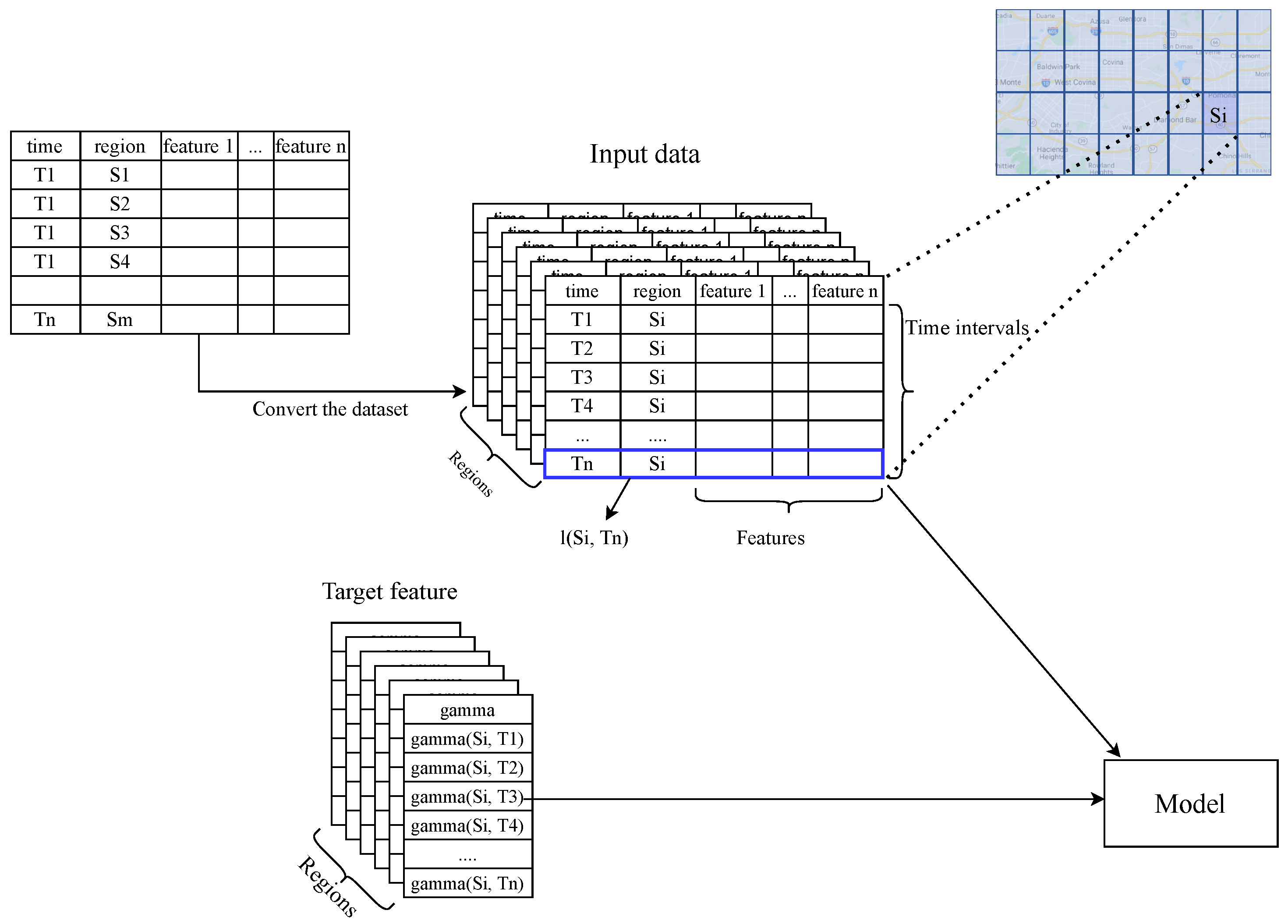
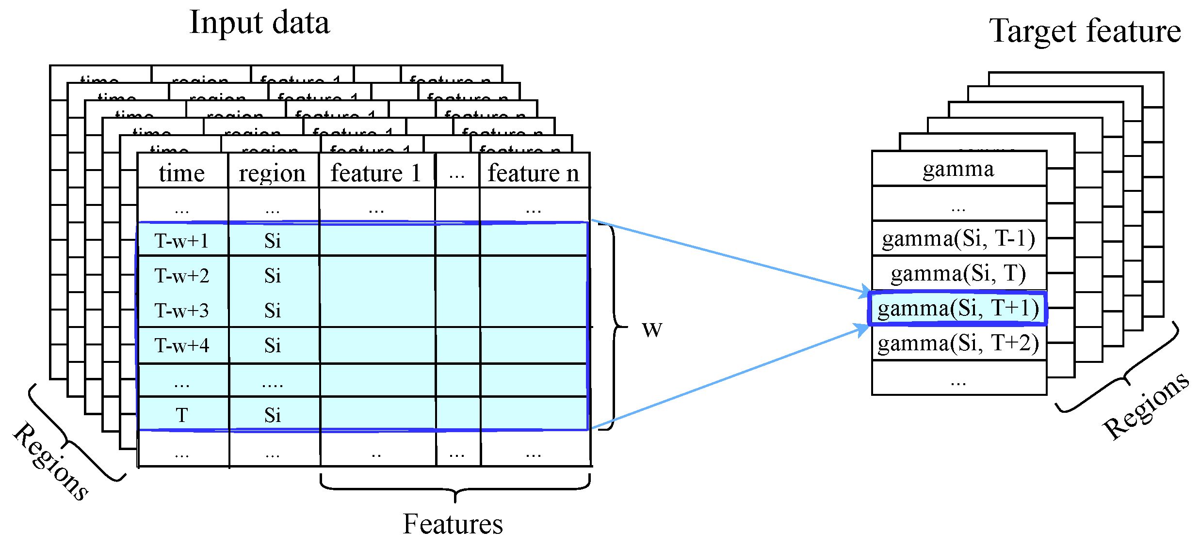
As described in Section 3.3, we create a vector representation $l(s,t)\in R^{26}$ for an accident in geographical region s during time interval t. Each vector has a corresponding Gammaclass label that indicates the intensity of delay in traffic flow after an accident. For accident-free data vectors, we label them as 0, which means no congestion is likely to take place. While this might not necessarily be true in the real world, it helps to simplify our problem formulation and label data vectors efficiently. The model predicts $gamma$ for time $t+1$ in region $s_i$ given a sequence of w previous time intervals in region $s_i$. Mathematically speaking, $gamm{a}_{(s_i,T+1)}$ is predicted given a sequence of $l(s_i,t),t\in \{T-w+1,T-w+2,\dots ,T\}.$ Figure 10 shows the process of converting the dataset to a 3D structure of $l(s_i,t)$ in the time and space domains. $Gammaclass$ is structured in the same order as $l(s_i,t)$. Figure 11 shows an arbitrary input sequence and its corresponding target in our 3D data structure.

We choose accidents from February 2019 to August 2019 as the training time frame. This 27-week time frame includes 13,026 accident representations and 319,194 non-accident representations. The frequency of each gammaclass is shown in Figure 12a, indicating that the data is highly imbalanced. Various methods exist to resolve the class imbalance problem in the context of classification or pattern recognition. Examples include (i) removing or merging data in the majority class, (ii) duplicating samples in minority classes, and (iii) adjusting the cost function to make misclassification of minority classes more costly than the misclassification of majority instances. In this study, the random under-sampling (RUS) method resulted in better outcomes. Hence, we use it to mitigate the class imbalance problem of $gammaclasses$. Using this approach, the ratio of accident to non-accident events increased from $1/43.3$ to $1/1.3$. Figure 12b shows the frequency of each $gammaclass$ after under-sampling. In addition, we assign a weight to each class in the loss function of models (and adjust them during training) to further address the imbalance issue. The following section describes class weighting in more detail.

5.3. Model Development

Since the distinction between accidents and non-accidents is difficult due to the complex factors that can affect traffic accidents, and some factors that cannot be observed and collected in advance (e.g., driver distraction), a model may not perform well on the distinction of $gammaclasses$ using single-step prediction (i.e., just by using a single model). Hence, we propose a cascade model that includes two deep neural network components. As a cascade model, the output of the first model is served as the input for the second model. The first component (referred to as a “layer” in our cascade design) focuses on distinguishing accidents from non-accident events; in other words, the first model detects if there will be an accident in the next two hours given w previous intervals’ information. If the first model classifies the input as an accident, then it goes to the second component. The second component focuses on accident impact prediction, i.e., $gammaclasses$) for accident events, detected by the previous layer. The structure of the proposed accident impact prediction model is shown in Figure 13. The structure of the two components in our design is described below.

(A) 

Label Prediction: The first model is a binary LSTM classifier that predicts whether the next interval would have an accident (i.e., label = 1) or not (i.e., label = 0).

We adopt a cascade modeling approach instead of a single-step classifier to decompose the task into two more focused subtasks: detecting the occurrence of accidents and then assessing their impact. This decoupled structure allows each model to specialize—Model 1 learns patterns for accident likelihood, while Model 2 focuses on severity estimation—leading to improved performance, especially in imbalanced and noisy settings. Moreover, this setup provides greater interpretability and flexibility, enabling separate tuning and the evaluation of detection and impact stages.

In accident prediction, it is vital that if an accident is likely to happen, the model can predict it in advance. Therefore, in the first model, the focus is on detecting accident events, and we use a weighting mechanism for this purpose, such that the weight of the accident class is higher than the weight of the non-accident class.

Class weights play a key role in guiding the model to compensate for the imbalance in the data, particularly by penalizing missed accident predictions more heavily than false alarms. There is no fixed theoretical formula for choosing class weights; they are typically treated as hyperparameters that must be tuned empirically. To this end, we conducted a grid search over a range of weight ratios from 1:1 up to 1:8 (non-accident/accident) and selected the combination that yielded the best precision–recall tradeoff on a validation set.

A similar process was applied to the second model, where we explored different weighting schemes to balance the three gamma classes (non-impact, medium-impact, and high-impact). The selected weights were those that minimized the misclassification of impactful accidents while keeping false positives low. Using grid search, we found the optimum weights to be 1 and 3 for non-accident and accident classes, respectively.

The first model takes as its input two components: (a) the index of a given zone $s_i$ (denoted as $inde{x}_{s_i}$), and (b) the temporal feature sequence $l(s_i,t)-inde{x}_{s_i}$, for $t\in \{T-w+1,T-w+2,\dots ,T\}$.

Here, “subtraction” indicates that the zone index is excluded from the temporal feature vectors. The first input is passed through an embedding layer of size $\left|R\right|\times 20$, where R is the set of all spatial grid cells, allowing the model to learn a distributed representation of regional characteristics such as spatial heterogeneity, traffic dynamics, and environmental context. The second input is a sequence of w vectors, each with 35 features, which is processed by two LSTM layers with 12 and 24 neurons, respectively. The resulting sequence encoding is concatenated with the embedded zone representation and passed through two fully connected layers, each with 25 neurons. Batch normalization is applied throughout the network to enhance convergence stability and reduce internal covariate shift. The structure of the first model is shown in Figure 14.

The overall architecture was selected through extensive hyperparameter tuning using a validation dataset. Simpler or shallower model variants were evaluated but failed to capture the complex temporal dependencies necessary for accurate accident prediction.

To mitigate overfitting, we employed batch normalization and early stopping, which are well-established regularization methods in deep learning. Although the chosen architecture introduces additional computational cost and longer training time, this trade-off was necessary to achieve improved predictive accuracy in the context of highly imbalanced and noisy real-world traffic data.

(B) 

Impact Prediction: The second model is a three-class CNN classifier that predicts $gammaclass$ for the next interval. The weight of each class is assigned based on its frequency and importance in our problem setup. Class imbalance in the impact prediction task can lead to biased predictions favoring the majority class (i.e., non-impact). To mitigate this, we incorporated class weights in the loss function to amplify the contribution of under-represented classes during training.

To determine the optimal set of weights, we conducted an extensive grid search over different configurations, varying the weights for $gammaclass=1$ and $gammaclass=2$ in the range of 1.0 to 5.0 (in increments of 0.5), while slightly adjusting the weight of $gammaclass=0$ around 0.5 to 1.0 to maintain baseline stability. This search aimed to balance the model’s sensitivity to impactful accidents (classes 1 and 2) with the need to avoid excessive false positives. The best-performing combination was selected based on validation set performance, prioritizing recall for impactful cases. The optimum weights are found to be 0.7, 4.5, and 3.5 for $gammaclass=0$, $gammaclass=1$ and $gammaclass=2$, respectively.

The second model is a CNN-based classifier that predicts the impact level (i.e., $gammaclass$) for intervals flagged as accident-prone by the first model. Although the input is primarily composed of samples predicted as accidents, we also include selected non-accident cases to help correct potential misclassifications from the first model and improve the cascade system’s overall reliability.

This CNN model consists of three convolutional layers followed by a flattening operation and three fully connected (dense) layers, with one dropout layer applied before the final two layers. The architecture is designed to extract hierarchical spatial and short-term temporal patterns from the input feature maps, enabling the model to differentiate between varying levels of post-accident impact. The specific configuration was determined through extensive hyperparameter tuning on a validation set. Simpler architectures with fewer convolutional layers or reduced capacity were tested but did not perform as well, particularly in capturing the nuances of medium- and high-impact events.

To mitigate overfitting and stabilize training, we included early stopping and dropout layers, both of which are widely used and effective in deep learning models [57]. While the depth of the network increases the training time, we found this to be an acceptable trade-off for improved performance. In future work, we aim to investigate lighter-weight alternatives such as MobileNet-style CNNs or dilated convolutions to reduce computational cost without compromising prediction quality.

The structure of the model is illustrated in Figure 15.

To the best of our knowledge, the proposed model is the first cascade model that can be applied in the real world to classify time intervals as accident and no-accident and then predict the severity of accidents using available data in real time. Additionally, given the type of data used, we believe that this model can be used in the real world to serve and make compelling predictions.

6. Experiments and Results

In this section, we first describe our evaluation metrics, then provide details on the experimental setup, and lastly present our results followed by discussions.

6.1. Evaluation Metrics

Failing to predict an accident event (and the consequent impact on traffic flow) is more costly comparing to the case of falsely forecasting traffic delay in an area as a result of a false accident prediction. Hence, we focus on two objectives: (1) maximizing confidence when predicting a non-accident case (i.e., $gammaclass=0$), and (2) minimizing the possibility of failing to predict accident events (i.e., cases with $gammaclass=1$ and $gammaclass=2$). In terms of metrics, these objectives can be translated to (1) “precision” for $gammaclass=0$ and (2) “recall” for $gammaclass=1$ and $gammaclass=2$. Precision and recall for multi-class classification are formulated as below:

$$Precisio{n}_{clas{s}_i}={\displaystyle \frac{M_{ii}}{{\sum }_i{M}_{ij}}}$$

(9)

$$Recal{l}_{clas{s}_i}={\displaystyle \frac{M_{ii}}{{\sum }_j{M}_{ij}}}$$

(10)

where $M_{ij}$ is the number of samples with the true class label i and predicted class label j. Therefore, we focus on precision for class “0” and recall for the other two classes for evaluation purposes. That being said, we still need to ensure reasonable recall for class “0” and acceptable precision for the other classes.

6.2. Experimental Setup

This section explains the experimental setup and the corresponding test runs. In this study, we used Keras, a Python-based Deep Learning library, to build the prediction models. We chose Adam [53] as the optimizer, given its characteristics to dynamically adjust the learning rate to converge faster and better. To find the optimal models’ settings, we performed a grid search over choices of LSTM layers, {1, 2, 3}, the number of neurons in recurrent layers, {12, 18, 24}, the number of fully-connected layers, {1, 2}, and the size of fully-connected layers, {12, 25, 50}, for the first model; and a grid search over choices of convolutional layers, {1, 2, 3}, and the number of filters in each convolutional layer, {8, 16, 32, 64, 128}, for the second model. The first model (i.e., LSTM) was trained for 150 epochs and the CNN model was trained for 25 epochs.

When building the input vectors, we can use past w intervals to build a vector and pass it to the cascade model to predict a label and a gamma class. But, what is the right choice of w? To answer this question, we ran an experiment on the test data to study the metrics introduced in the previous section on different classes for different choices of w. The results are shown in Figure 16. According to these results, a choice of 4 or 5 for w (which translates to having information from 8 to 10 h before the accident) seems to be reasonable for this parameter. Here, we chose to set $w=4$, since it consistently provides reasonable results over all three gamma classes.

6.3. Baseline Models

In this section, random forest (RF), gradient boosting classifier (GBC), a CNN, and an LSTM are selected as the baseline algorithms. RF and GBC are traditional models that generally provide satisfactory results on a variety of classification or regression problems. Furthermore, as our proposed cascade model leverages LSTM and CNN components, the use of these two as standalone models seems to be a reasonable choice. We used Scikit-learn and Keras for the off-the-shelf implementation of the baseline models. As for hyperparameters, for the random forest, we used 200 estimators, the maximum depth was 12, the minimum sample split was 2, and the rest of the parameters were set to the default values. For GBC, we used 300 estimators, the learning rate was 0.8, the maximum depth was 2, and the rest of the parameters were set to the default values. The baseline CNN and LSTM models share the same structure as in the proposed cascade model, except for the last layer of the LSTM that uses 3 neurons instead of 2 (since by means of this model we seek to predict three $gammaclasses$ in a single step).

6.4. Results and Model Comparison

This section provides the evaluation results based on test data (from September 2019 to November 2019) to compare our proposal against the two traditional (i.e., RF and GBC) and deep neural network models (i.e., CNN and LSTM). A summary of the results is presented in

Table 8. Accident impact prediction results based on precision for $gammaclass=0$ and recall for $gammaclasses$ 1 and 2.

Models	Precision Class 0	Precision Class 1	Precision Class 2	Recall Class 0	Recall Class 1	Recall Class 2
Gradient Boosting	0.92	0.14	0.04	0.81	0.14	0.23
Random Forest	0.93	0.13	0.05	0.69	0.31	0.30
LSTM	0.94	0.10	0.04	0.56	0.34	0.36
CNN	0.94	0.12	0.04	0.11	0.32	0.32
Cascade Model	0.96	0.10	0.04	0.31	0.41	0.50

and Figure 17. From these results, we can see that the GBC model performed quite well in detecting non-accident events (i.e., $gammaclass$ = 0) based on precision for this class. However, its results in predicting the other two classes are not satisfactory.

Further, the RF model does a better job in detecting accidents with medium or high impact. The LSTM model seems to perform better than the other models (except the cascaded model) in detecting accidents with medium or high impact, indicating the importance of taking into account the temporal dependencies to encode input data better. However, CNN’s performance is not satisfactory as a single-step model.

While the proposed cascade model provides satisfactory results in terms of precision for $gammaclass$ = 0, it results in significantly higher recalls when predicting the other two classes. These are important observations, because in the case of accident prediction, failing to predict the occurrence of an accident in a zone (i.e., low recall) can result in a more serious outcome than falsely predicting an accident in a non-accidental zone (i.e., low precision). Therefore, we generally care more about having higher recall to predict impact for accident events, and also a high precision to decide whether a time interval is associated with an accident event or not. Please note that while high precision is still necessary for non-zero classes (i.e., cases with reported accident), a real-world framework must ensure acceptable recall for these cases.

6.5. Influencing Factor Analysis

In this section, we conduct an analysis to study the importance of different factors in our model design (i.e., components and input features). Such analysis can help to improve our input features and model design, all in order to build an effective framework for real-world applications.

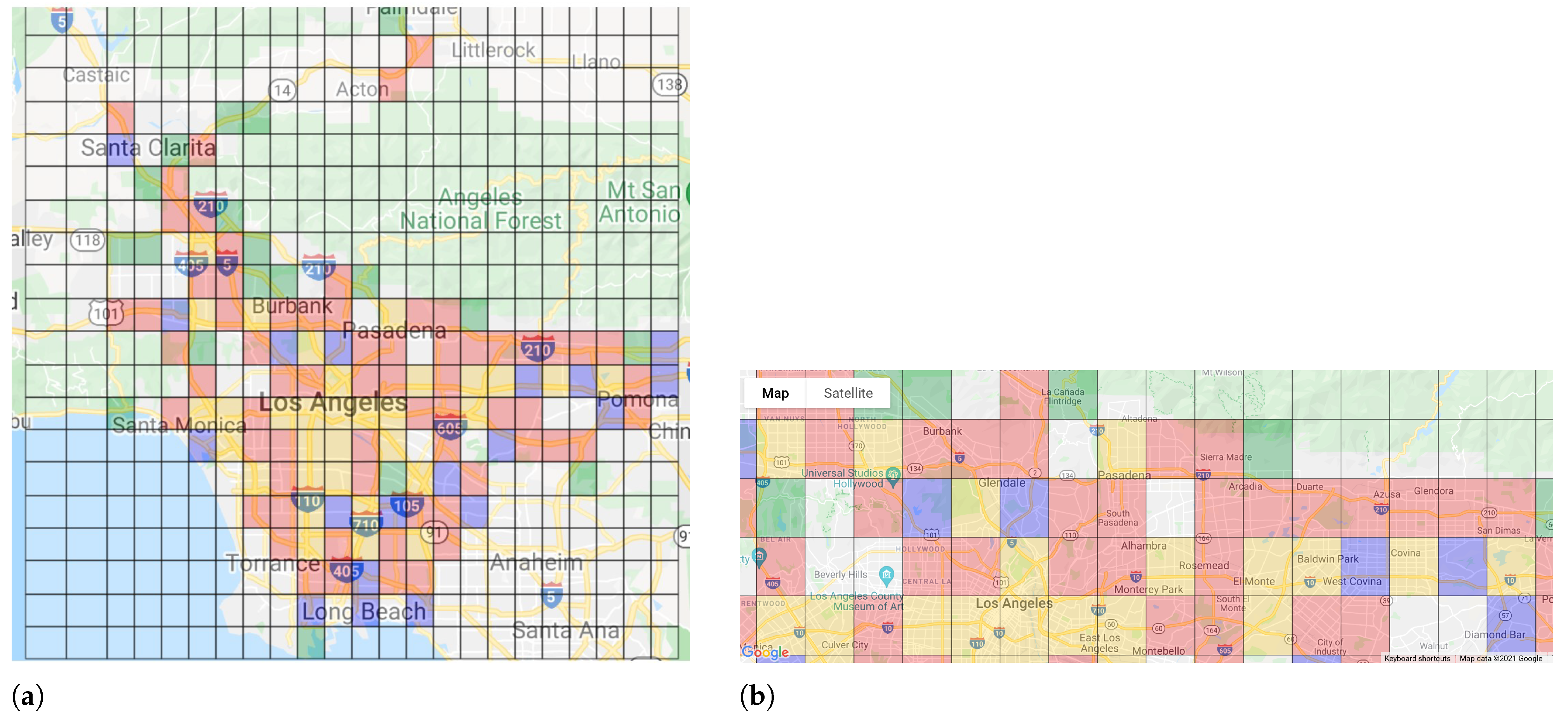
(A) Latent Location Representations: As discussed in Section 3.1 and Section 5.2, our dataset covers accident events in an extensive area containing urban road network and high-speed roads. During the model training, we derive latent representations for each region to encode essential spatiotemporal characteristics. The first analysis aims to study the quality of derived representations and understand how they can help to distinguish between regions (or zones) with different spatial characteristics. We believe that these latent representations can show how well the model has learned spatial factors involved in post-accident impacts. Therefore, we clustered latent (or embedding) vectors into four clusters and specified each cluster with a specific color on a map for better interpretation. Figure 18 shows the results of this analysis. Based on Figure 18a, most of the adjacent regions in our study area are found to be in the same cluster, indicating that they share the same accident-related characteristics, which is aligned with the principals of urban design. As we move away from the center to the outskirts of the county area, we see more heterogeneity in clusters. This could either be a result of fewer accident reports (i.e., less data for the model to train on and properly distinguish between regions) or more heterogeneity in the road network in the suburbs. Figure 18b shows more details of different clusters. We can see that urban highways are mainly highlighted in yellow, while areas with a sparse road network are highlighted in green. Blue and red regions are mostly urban regions with a high density of spatial points of interest (e.g., intersections), and the difference between them may be in the intensity of traffic congestion caused by accidents.

In summary, the research findings in this section indicate the ability of our framework to build meaningful latent representations for different regions, that help to better predict accidents and their impact. Moreover, different clusters seem to reasonably represent regions with similar characteristics. The yellow cluster mostly represents regions with a concentration of arterial highways (for which we can expect higher delays as a result of an accident). The green cluster, in contrast, represents regions with marginal and low traffic flow, and thus an accident in these regions will not cause as much delay as we would expect for regions in yellow cluster. For the regions in the red cluster, we can expect less delay (or impact) due to lower traffic flow, but higher delay in comparison to the regions in the blue cluster. Also note that regions with a sparse road network and low traffic flow (green regions) are mostly located in the suburbs and locations far from downtown areas.

(B) Ablation study: The second analysis is an ablation study aiming to explore the importance of each feature category when used individually for predicting accident impact. Here, we study three categories of features—weather, spatial, and accident information—and compare their results with the case of using all categories of features. By systematically evaluating model performance with each category—weather, spatial, and accident information—used in isolation, we assess the extent to which each group contributes unique and complementary information to overall prediction accuracy. Figure 19 shows the analysis results, and it reveals that removing all but one feature category would significantly degrade the prediction results. In comparison to the best model results, using each category alone as an input would result in greater recall for $gammaclass$ = 2, lower recall for $gammaclass$ = 1, and almost the same precision for $gammaclass$ = 0 (except for the weather category). It is worth noting that using just weather features does not assist in identifying cases where $gammaclass$ = 0. This can either indicate that the quality of weather data in our dataset is not as good as it should be (e.g., it could be finer-grained spatially and temporally), or that weather characteristics do not play an important role in the area of our study (throughout the year, we do not usually see significant shifts in weather conditions in the Los Angeles area (see https://weatherspark.com/y/1705/Average-Weather-in-Los-Angeles-California-United-States-Year-Round (accessed on 3 June 2025) for more details)). This analysis demonstrates that effective accident impact prediction relies on the integration of all feature categories, as the exclusion of any single group yields a marked decline in model performance. The ablation results support the conclusion that weather, spatial, and accident information each provide distinct, complementary signals that are essential for maximizing predictive accuracy across different impact classes.

While this study evaluates the importance of grouped features, we acknowledge that further investigation of individual feature contributions could provide deeper interpretability, and we propose this as a direction for future work.

7. Conclusions and Future Work

Traffic accidents are serious public safety concerns, and many studies have focused on analyzing and predicting these infrequent events. However, existing studies suffer from employing extensive data that may not be easily available to other researchers or recorded in real time, meaning they cannot be utilized for real-world applications. Additionally, they fail to establish an appropriate criterion for determining the impact of accidents. To overcome these limitations, this study proposes a cascade model that combines LSTM and CNN components for real-time traffic accident prediction. The model detects future accidents and assesses their impact on surrounding traffic flow using a novel metric called gamma. Four complementary datasets, including accident data, congestion data, weather data, and spatial data, are utilized to construct the input data. Through extensive experiments conducted using data from Los Angeles county, we demonstrate that our proposed model outperforms existing approaches in terms of precision for cases with minimal impact (i.e., no reported accidents, $gammaclass$ = 0) and recall for cases with significant impact (i.e., reported accidents, $gammaclass$ = 1 and 2).

This study has several implications for future research. Firstly, we suggest expanding the framework to incorporate data from neighboring regions to predict accident impact for a target region, mitigating data sparsity. Additionally, the inclusion of satellite imagery data to enhance the model’s ability to distinguish between regions and capture spatial information could also improve performance. Future works may also consider physical or human consequences—such as injuries, fatalities, or emergency response needs—as part of accident impact, provided that reliable real-time data for these outcomes becomes available.

While our work makes important contributions, it is important to note its limitations. Our model currently only classifies accident impacts into three broad categories. Future research could benefit from more granular classifications or assigning probabilities to each accident’s potential impact on road conditions. Additionally, the accuracy of our results may have been limited by the accessibility and quality of the weather data we used from a private source, which was gathered from only four airports. To enhance the accuracy of our model, future research could incorporate radar data or other more comprehensive weather data sources. Addressing these limitations will be essential to advancing our understanding of the factors that contribute to road accidents and improving road safety.

Overall, this study provides a promising approach to real-time traffic accident prediction using a novel metric for measuring accident impact. The proposed framework has the potential to be applied in real-world settings to enhance public safety and traffic management.

References

1. Wang, C.; Li, X.; Zhou, X.; Wang, A.; Nedjah, N. Soft computing in big data intelligent transportation systems. Appl. Soft Comput. 2016, 38, 1099–1108. [Google Scholar] [CrossRef]
2. Zhang, J.; Wang, J.; Fang, S. Prediction of urban expressway total traffic accident duration based on multiple linear regression and artificial neural network. In Proceedings of the 2019 5th International Conference on Transportation Information and Safety (ICTIS), Liverpool, UK, 14–17 July 2019; pp. 503–510. [Google Scholar]
3. Austin, R.D.; Carson, J.L. An alternative accident prediction model for highway-rail interfaces. Accid. Anal. Prev. 2002, 34, 31–42. [Google Scholar] [CrossRef] [PubMed]
4. Oyedepo, O.; Makinde, O. Accident Prediction Models for Akure–Ondo Carriageway, Ondo State Southwest Nigeria; Using Multiple Linear Regressions. Afr. Res. Rev. 2010, 4, 30–49. [Google Scholar] [CrossRef]
5. Wei, C.H.; Lee, Y. Sequential forecast of incident duration using artificial neural network models. Accid. Anal. Prev. 2007, 39, 944–954. [Google Scholar] [CrossRef]
6. Salahadin Seid Yassin, P. Road accident prediction and model interpretation using a hybrid K-means and random forest algorithm approach. SN Appl. Sci. 2020, 1576. [Google Scholar]
7. Sarkar, S.; Vinay, S.; Raj, R.; Maiti, J.; Mitra, P. Application of optimized machine learning techniques for prediction of occupational accidents. Comput. Oper. Res. 2019, 106, 210–224. [Google Scholar] [CrossRef]
8. Wenqi, L.; Dongyu, L.; Menghua, Y. A model of traffic accident prediction based on convolutional neural network. In Proceedings of the 2017 2nd IEEE International Conference on Intelligent Transportation Engineering (ICITE), Singapore, 1–3 September 2017; pp. 198–202. [Google Scholar]
9. Ozbayoglu, M.; Kucukayan, G.; Dogdu, E. A real-time autonomous highway accident detection model based on big data processing and computational intelligence. In Proceedings of the 2016 IEEE International Conference on Big Data (Big Data), Washington, DC, USA, 5–8 December 2016; pp. 1807–1813. [Google Scholar]
10. Marcillo, P.; Valdivieso Caraguay, Á.L.; Hernández-Álvarez, M. A systematic literature review of learning-based traffic accident prediction models based on heterogeneous sources. Appl. Sci. 2022, 12, 4529. [Google Scholar] [CrossRef]
11. Li, P.; Abdel-Aty, M.; Yuan, J. Real-time crash risk prediction on arterials based on LSTM-CNN. Accid. Anal. Prev. 2020, 135, 105371. [Google Scholar] [CrossRef] [PubMed]
12. Moosavi, S.; Samavatian, M.H.; Nandi, A.; Parthasarathy, S.; Ramnath, R. Short and Long-Term Pattern Discovery Over Large-Scale Geo-Spatiotemporal Data. In Proceedings of the 25th ACM SIGKDD International Conference on Knowledge Discovery & Data Mining, KDD ’19, Anchorage, AK, USA, 4–8 August 2019; pp. 2905–2913. [Google Scholar] [CrossRef]
13. Caliendo, C.; Guida, M.; Parisi, A. A crash-prediction model for multilane roads. Accid. Anal. Prev. 2007, 39, 657–670. [Google Scholar] [CrossRef]
14. Najjar, A.; Kaneko, S.; Miyanaga, Y. Combining satellite imagery and open data to map road safety. In Proceedings of the AAAI Conference on Artificial Intelligence, San Francisco, CA, USA, 4–9 February 2017; Volume 31. [Google Scholar]
15. Ren, H.; Song, Y.; Wang, J.; Hu, Y.; Lei, J. A deep learning approach to the citywide traffic accident risk prediction. In Proceedings of the 2018 21st International Conference on Intelligent Transportation Systems (ITSC), Maui, HI, USA, 4–7 November 2018; pp. 3346–3351. [Google Scholar]
16. Yuan, Z.; Zhou, X.; Yang, T. Hetero-convlstm: A deep learning approach to traffic accident prediction on heterogeneous spatio-temporal data. In Proceedings of the 24th ACM SIGKDD International Conference on Knowledge Discovery & Data Mining, London, UK, 19–23 August 2018; pp. 984–992. [Google Scholar]
17. Chen, Q.; Song, X.; Yamada, H.; Shibasaki, R. Learning deep representation from big and heterogeneous data for traffic accident inference. In Proceedings of the AAAI Conference on Artificial Intelligence, Phoenix, AZ, USA, 12–17 February 2016; Volume 30. [Google Scholar]
18. Yu, R.; Abdel-Aty, M. Utilizing support vector machine in real-time crash risk evaluation. Accid. Anal. Prev. 2013, 51, 252–259. [Google Scholar] [CrossRef]
19. Lin, L.; Wang, Q.; Sadek, A.W. A novel variable selection method based on frequent pattern tree for real-time traffic accident risk prediction. Transp. Res. Part C Emerg. Technol. 2015, 55, 444–459. [Google Scholar] [CrossRef]
20. Bianchi, F.M.; Maiorino, E.; Kampffmeyer, M.C.; Rizzi, A.; Jenssen, R. Recurrent Neural Networks for Short-Term Load Forecasting: An Overview and Comparative Analysis; Springer: Cham, Switzerland, 2017. [Google Scholar]
21. Tian, Y.; Pan, L. Predicting short-term traffic flow by long short-term memory recurrent neural network. In Proceedings of the 2015 IEEE International Conference on Smart city/SocialCom/SustainCom (SmartCity), Chengdu, China, 19–21 December 2015; pp. 153–158. [Google Scholar]
22. Parsa, A.B.; Chauhan, R.S.; Taghipour, H.; Derrible, S.; Mohammadian, A. Applying Deep Learning to Detect Traffic Accidents in Real Time Using Spatiotemporal Sequential Data. arXiv 2019, arXiv:1912.06991. [Google Scholar] [CrossRef]
23. Wang, X.; Chai, Y.; Li, H.; Wang, W.; Sun, W. Graph Convolutional Network-based Model for Incident-related Congestion Prediction: A Case Study of Shanghai Expressways. ACM Trans. Manag. Inf. Syst. 2021, 12, 21. [Google Scholar] [CrossRef]
24. Bao, J.; Liu, P.; Ukkusuri, S.V. A spatiotemporal deep learning approach for citywide short-term crash risk prediction with multi-source data. Accid. Anal. Prev. 2019, 122, 239–254. [Google Scholar] [CrossRef]
25. Singh, G.; Pal, M.; Yadav, Y.; Singla, T. Deep neural network-based predictive modeling of road accidents. Neural Comput. Appl. 2020, 32, 12417–12426. [Google Scholar] [CrossRef]
26. Theofilatos, A.; Chen, C.; Antoniou, C. Comparing machine learning and deep learning methods for real-time crash prediction. Transp. Res. Rec. 2019, 2673, 169–178. [Google Scholar] [CrossRef]
27. Moosavi, S.; Samavatian, M.H.; Parthasarathy, S.; Teodorescu, R.; Ramnath, R. Accident risk prediction based on heterogeneous sparse data: New dataset and insights. In Proceedings of the 27th ACM SIGSPATIAL International Conference on Advances in Geographic Information Systems, Chicago, IL, USA, 5–8 November 2019; pp. 33–42. [Google Scholar]
28. Chen, C.; Fan, X.; Zheng, C.; Xiao, L.; Cheng, M.; Wang, C. Sdcae: Stack denoising convolutional autoencoder model for accident risk prediction via traffic big data. In Proceedings of the 2018 Sixth International Conference on Advanced Cloud and Big Data (CBD), Lanzhou, China, 12–15 August 2018; pp. 328–333. [Google Scholar]
29. Kaffash Charandabi, N.; Gholami, A.; Abdollahzadeh Bina, A. Road accident risk prediction using generalized regression neural network optimized with self-organizing map. Neural Comput. Appl. 2022, 34, 8511–8524. [Google Scholar] [CrossRef]
30. Parsa, A.B.; Movahedi, A.; Taghipour, H.; Derrible, S.; Mohammadian, A.K. Toward safer highways, application of XGBoost and SHAP for real-time accident detection and feature analysis. Accid. Anal. Prev. 2020, 136, 105405. [Google Scholar] [CrossRef]
31. Khattak, A.J.; Schofer, J.L.; Wang, M.H. A simple time sequential procedure for predicting freeway incident duration. J. Intell. Transp. Syst. 1995, 2, 113–138. [Google Scholar] [CrossRef]
32. Garib, A.; Radwan, A.; Al-Deek, H. Estimating magnitude and duration of incident delays. J. Transp. Eng. 1997, 123, 459–466. [Google Scholar] [CrossRef]
33. Peeta, S.; Ramos, J.L.; Gedela, S. Providing Real-Time Traffic Advisory and Route Guidance to Manage Borman Incidents On-Line Using the Hoosier Helper Program; Indiana Department of Transportation and Purdue University: West Lafayette, IN, USA, 2000. [Google Scholar]
34. Yu, B.; Xia, Z. A methodology for freeway incident duration prediction using computerized historical database. In CICTP 2012: Multimodal Transportation Systems—Convenient, Safe, Cost-Effective, Efficient, Proceedings of the 12th COTA International Conference of Transportation Professionals, Beijing, China, 3–6 August 2012; American Society of Civil Engineers: Reston, VA, USA, 2012; pp. 3463–3474. [Google Scholar]
35. Wang, W.; Chen, H.; Bell, M.C. Vehicle breakdown duration modeling. J. Transp. Stat. 2005, 8, 75. [Google Scholar]
36. Vlahogianni, E.I.; Karlaftis, M.G. Fuzzy-entropy neural network freeway incident duration modeling with single and competing uncertainties. Comput.-Aided Civ. Infrastruct. Eng. 2013, 28, 420–433. [Google Scholar] [CrossRef]
37. Yu, B.; Wang, Y.; Yao, J.; Wang, J. A comparison of the performance of ANN and SVM for the prediction of traffic accident duration. Neural Netw. World 2016, 26, 271. [Google Scholar] [CrossRef]
38. Ma, X.; Ding, C.; Luan, S.; Wang, Y.; Wang, Y. Prioritizing influential factors for freeway incident clearance time prediction using the gradient boosting decision trees method. IEEE Trans. Intell. Transp. Syst. 2017, 18, 2303–2310. [Google Scholar] [CrossRef]
39. Yu, R.; Li, Y.; Shahabi, C.; Demiryurek, U.; Liu, Y. Deep learning: A generic approach for extreme condition traffic forecasting. In Proceedings of the 2017 SIAM International Conference on Data Mining, Houston, TX, USA, 27–29 April 2017; pp. 777–785. [Google Scholar]
40. Lin, Y.; Li, R. Real-time traffic accidents post-impact prediction: Based on crowdsourcing data. Accid. Anal. Prev. 2020, 145, 105696. [Google Scholar] [CrossRef]
41. Zhang, S.; Liu, H.; Yang, Y.; Zhang, S.; Zhang, Z.; Wang, C.; Wang, M. Prediction of traffic accident impact range based on CatBoost ensemble algorithm. In Proceedings of the Second International Conference on Algorithms, Microchips, and Network Applications (AMNA 2023), Zhengzhou, China, 13–15 January 2023; Volume 12635, pp. 7–11. [Google Scholar]
42. Ekanem, I. Analysis of Road Traffic Accident Using AI Techniques. Open J. Saf. Sci. Technol. 2025, 15, 36–56. [Google Scholar] [CrossRef]
43. Moosavi, S.; Samavatian, M.H.; Parthasarathy, S.; Ramnath, R. A countrywide traffic accident dataset. arXiv 2019, arXiv:1906.05409. [Google Scholar] [CrossRef]
44. Xing, F.; Huang, H.; Zhan, Z.; Zhai, X.; Ou, C.; Sze, N.; Hon, K. Hourly associations between weather factors and traffic crashes: Non-linear and lag effects. Anal. Methods Accid. Res. 2019, 24, 100109. [Google Scholar] [CrossRef]
45. Malin, F.; Norros, I.; Innamaa, S. Accident risk of road and weather conditions on different road types. Accid. Anal. Prev. 2019, 122, 181–188. [Google Scholar] [CrossRef] [PubMed]
46. Fountas, G.; Fonzone, A.; Gharavi, N.; Rye, T. The joint effect of weather and lighting conditions on injury severities of single-vehicle accidents. Anal. Methods Accid. Res. 2020, 27, 100124. [Google Scholar] [CrossRef]
47. Doane, D.P. Aesthetic frequency classifications. Am. Stat. 1976, 30, 181–183. [Google Scholar] [CrossRef]
48. Skabardonis, A.; Varaiya, P.; Petty, K.F. Measuring recurrent and nonrecurrent traffic congestion. Transp. Res. Rec. 2003, 1856, 118–124. [Google Scholar] [CrossRef]
49. Lv, Y.; Tang, S.; Zhao, H. Real-time highway traffic accident prediction based on the k-nearest neighbor method. In Proceedings of the 2009 International Conference on Measuring Technology and Mechatronics Automation, Zhangjiajie, China, 11–12 April 2009; Volume 3, pp. 547–550. [Google Scholar]
50. Wang, C.; Quddus, M.; Ison, S. A spatio-temporal analysis of the impact of congestion on traffic safety on major roads in the UK. Transp. A Transp. Sci. 2013, 9, 124–148. [Google Scholar] [CrossRef]
51. Sánchez González, S.; Bedoya-Maya, F.; Calatayud, A. Understanding the Effect of Traffic Congestion on Accidents Using Big Data. Sustainability 2021, 13, 7500. [Google Scholar] [CrossRef]
52. Zheng, Z.; Wang, Z.; Zhu, L.; Jiang, H. Determinants of the congestion caused by a traffic accident in urban road networks. Accid. Anal. Prev. 2020, 136, 105327. [Google Scholar] [CrossRef]
53. Kingma, D.P.; Ba, J. Adam: A method for stochastic optimization. arXiv 2014, arXiv:1412.6980. [Google Scholar]
54. Yuan, J.; Abdel-Aty, M.; Gong, Y.; Cai, Q. Real-time crash risk prediction using long short-term memory recurrent neural network. Transp. Res. Rec. 2019, 2673, 314–326. [Google Scholar] [CrossRef]
55. Ounoughi, C.; Yahia, S.B. Sequence to sequence hybrid Bi-LSTM model for traffic speed prediction. Expert Syst. Appl. 2024, 236, 121325. [Google Scholar] [CrossRef]
56. Yang, B.; Sun, S.; Li, J.; Lin, X.; Tian, Y. Traffic flow prediction using LSTM with feature enhancement. Neurocomputing 2019, 332, 320–327. [Google Scholar] [CrossRef]
57. Ying, X. An overview of overfitting and its solutions. J. Phys. Conf. Ser. 2019, 1168, 022022. [Google Scholar] [CrossRef]
58. Yu, B.; Yin, H.; Zhu, Z. Spatio-temporal graph convolutional networks: A deep learning framework for traffic forecasting. arXiv 2017, arXiv:1709.04875. [Google Scholar]
59. Hochreiter, S.; Schmidhuber, J. Long short-term memory. Neural Comput. 1997, 9, 1735–1780. [Google Scholar] [CrossRef] [PubMed]
60. Wang, J.; Wang, B.; Zhou, S.; Li, C. Prediction Model for Traffic Congestion Based on the Deep Learning of Convolutional Neural Network. In CICTP 2017: Transportation Reform and Change—Equity, Inclusiveness, Sharing, and Innovation, Proceedings of the 17th COTA International Conference of Transportation Professionals, Shanghai, China, 7–9 July 2017; American Society of Civil Engineers: Reston, VA, USA, 2018; pp. 2494–2505. [Google Scholar]
Figure 1. Overall research workflow for accident impact prediction.
Urbansci 09 00299 g001
Figure 2. Spatial dispersion of accident locations in Los Angeles County (2016–2020).
Urbansci 09 00299 g002
Figure 3. Forming a feature vector at time t in region s based on heterogeneous data obtained from various data sources.
Urbansci 09 00299 g003
Figure 4. Four best-fitted distributions on accident duration data and their summation of squared estimate of errors.
Urbansci 09 00299 g004
Figure 5. Distribution of severity values in the accident dataset. Severity is an ordinal variable ranging from 1 to 4, representing the level of impact on traffic rather than physical injury or property damage as defined by the dataset providers. Severity 1 = least impact; Severity 2 = minor or manageable delay; Severity 3 = moderate or extended delay; Severity 4 = significant traffic disruption.
Urbansci 09 00299 g005
Figure 6. The process of fitting F on congestion events and applying it to accident events to predict impact (i.e., γ ).
Urbansci 09 00299 g006
Figure 7. LSTM unit structure.
Urbansci 09 00299 g007
Figure 8. Overall structure of the convolution neural network.
Urbansci 09 00299 g008
Figure 9. Illustration of key components in a convolutional neural network. (a) Convolution layer structure. (b) Pooling layer operation.
Urbansci 09 00299 g009
Figure 10. Converting dataset into a 3D structure of l ( s i , t ) and G a m m a c l a s s in the time and space domains. Model inputs and outputs are extracted from this 3D structure.
Urbansci 09 00299 g010
Figure 11. A sequence of l ( s i , t ) , t { T w + 1 , T w + 2 , , T } as model input and G a m m a c l a s s ( s i , T + 1 ) as its corresponding target feature.
Urbansci 09 00299 g011
Figure 12. Comparing frequency distribution of gamma classes before and after random under sampling.
Urbansci 09 00299 g012
Figure 13. Cascade model overview; the first model predicts whether the next interval will have an accident (i.e., label = 1) or not (i.e., label = 0). Next, predictions with label = 1 are given to the second model that predicts the intensity of accident impact (i.e., g a m m a c l a s s ). Non-accident predictions of the first model are labeled as g a m m a c l a s s = 0 .
Urbansci 09 00299 g013
Figure 14. Structure of the first model (layer) in the cascade model. The index of a given zone is fed into an embedding layer to extract latent features for that zone during training. The other features (e.g., weather conditions and congestion data) are fed into LSTM layers. The output of the aforementioned layers is then concatenated and input to fully connected layers to predict the possibility of an accident.
Urbansci 09 00299 g014
Figure 15. Structure of the second model (layer) in the cascade model; three consecutive convolutional layers are used to extract spatial latent features from data, and then three fully connected layers are used to convert the output of convolutional layers to a probability vector for g a m m a classes.
Urbansci 09 00299 g015
Figure 16. Comparison of evaluation metrics (i.e., recall for classes 1 and 2 and precision for class 0) based on the cascade model for different choices of input length (or window size).
Urbansci 09 00299 g016
Figure 17. Comparing different models based on precision and recall to predict gammaclasses 0, 1, and 2.
Urbansci 09 00299 g017
Figure 18. (a) An overview of different clusters of latent representations of regions. (b) Closer look at clustering of different regions and their spatial characteristics. Clustering of latent spatial representations for different regions based on road network and spatial context. Each region is colored according to its cluster assignment, derived from the embedding layer of the trained model. Yellow clusters correspond to areas dominated by arterial highways and high-speed roads. Green regions represent areas with sparse road networks and low traffic volume, typically located in suburban zones. Blue and red clusters mostly represent urban areas with dense road networks and a high concentration of spatial points of interest (e.g., intersections), with variation likely driven by differences in congestion intensity or connectivity. Transparent areas are regions excluded due to insufficient data.
Urbansci 09 00299 g018
Figure 19. Model performance based on evaluation metrics (recall of g a m m a c l a s s = 1 , 2 ; precision of g a m m a c l a s s = 0 ) when using just one feature category (i.e., weather features, spatial features, and accident-related features) in comparison to the case of using all feature categories as the input.
Urbansci 09 00299 g019