Predictive Modeling of Urban Travel Demand Using Neural Networks and Regression Analysis

Abstract

Urban transportation systems are increasingly strained by population growth, changing mobility patterns, and the need for sustainable infrastructure planning. The accurate modeling of urban trip generation is critical for effective and sustainable transportation planning, especially in the context of rapidly growing urban populations and evolving travel behaviors. This study investigated the application of advanced statistical methods and artificial intelligence-based techniques for forecasting urban travel demand. Erzincan, with a population of approximately 200,000, serves as a representative mid-sized city, offering valuable insights for transportation planning and traffic management. Data collected from various user groups, including households and university students, provide a comprehensive understanding of local travel behavior. Four predictive modeling techniques, linear regression, Poisson regression, negative binomial regression, and artificial neural networks (ANNs), were applied to the dataset, followed by a comparative performance evaluation. Additionally, a macro-level simulation was conducted using VISUM (Release 18.2.22) software to evaluate the current transportation network and assess the potential impacts of proposed improvement scenarios. The results show that the ANN model provided the highest predictive accuracy for household-based data (R² = 0.62), while the linear regression model yielded the best results for dormitory-based data (R² = 0.95). Furthermore, Poisson regression proved most effective in estimating the minimum trip generation time, which was estimated to be 22.77 min under simulated conditions. The study offers practical insights for transport planners and policymakers by demonstrating how predictive analytics and simulation tools can be integrated to address urban mobility challenges.

1. Introduction

The current road infrastructure is insufficient due to the fast-growing population and the corresponding growth in individual vehicle ownership. As a result, transportation systems should be developed to be comfortable and safe [1]. In this environment, it is critical to forecast current and future traffic growth and develop an appropriate transportation strategy. Transportation planning is a process that generates data that will aid decision makers in the construction of future transportation networks. It can also be defined as a tool or method for a sustainable planning approach that analyzes and evaluates the current state of urban transportation infrastructure; determines future (target year and/or years) investments, regulations, and operational approaches; and generates predictions [2]. Transportation planning should be carried out by relating them from the largest to the smallest towns across the country or from the macro- to the micro-level.

As the number of motor vehicles increased in the early 20th century, researchers conducted the first residential and roadside pedestrian surveys in the 1920s and 1930s to help control congested streets and crossings. They utilized this knowledge to develop street widening and one-way street designs. In the early 1940s, individuals in the United States thought that transportation planning was limited to technical solutions to crowded junctions. However, by the 1950s, it had become regarded as a systematic study that considered not only intersection designs but also changes in urban transportation plans, population growth, and vehicle ownership. In the 1970s, a process that also addressed technical and political issues for transportation planning in cities was observed to begin [3].

In the 1990s, the concept of sustainability for transportation emerged, aiming to ensure the efficient transportation of people, goods (things), and services and to leave a less damaged environmental and cultural heritage for the future. Although the first transportation planning models only considered cost-effectiveness, later studies focused on economics, land use, and the management of transportation systems [4]. Instead of temporary and costly designs, transportation planners must prepare for the future in terms of delivering both economic and long-term services, as well as resolving potential bad events in a predictable manner. Recent research has resulted in methods for addressing traffic issues in future cities. These transportation planning studies strive to develop a sustainable and successful transportation network.

Purpose of Study

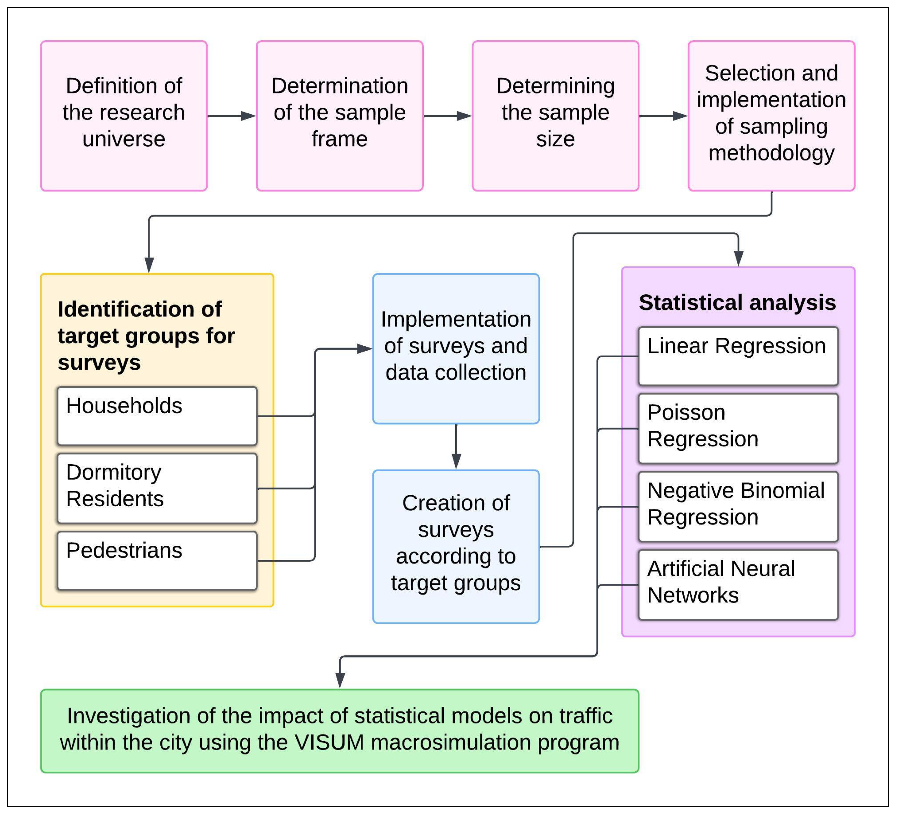
This study primarily aims to develop a sustainable urban transportation plan for Erzincan, a city of strategic importance with strong growth potential. While existing research on urban transportation planning predominantly focuses on large metropolitan areas, data-driven planning efforts in small- to medium-sized cities like Erzincan, still in the process of development, remain significantly limited. This study addresses that gap by contributing to the development of a locally applicable, data-based modeling approach.

To support travel demand forecasting and trip distribution analysis, household and dormitory students surveys were conducted to ensure a diverse representation of traveler types, resulting in a comprehensive set of primary data. Moreover, studies that employ multiple statistical modeling techniques in parallel, as conducted in this research, are rare in the current literature. Using these data, four different models were created and compared using artificial neural networks (ANNs), Poisson regression (PR), negative binomial regression (NBREG), and multiple linear regression (MLR) statistical methods.

Additionally, the integration of field-collected data with an advanced simulation tool such as PTV VISUM has significantly broadened this study’s scope. As a result, areas of severe traffic congestion in Erzincan were accurately identified, and the feasibility of targeted improvement strategies was comprehensively evaluated.

This study contains five sections: The first section is the “Introduction”. The second section, “Literature Review”, provides a comprehensive overview of recent developments in artificial intelligence, data analytics, and simulation technologies as applied to transportation systems. The third section, “Materials and Methods”, provides detailed information about the study area, data collection methods, and the surveys conducted. Additionally, technical details regarding the macro-level simulation studies are presented in this section. The fourth section, “Results and Discussion”, presents the findings of the statistical models developed using data obtained from surveys conducted with households and dormitory students. The results are discussed in detail, and origin–destination (O-D)-based travel times between each traffic zone are calculated and thoroughly analyzed as part of the macro-simulation studies. In the fifth section, “Conclusions”, the overall findings of the study are summarized, and various recommendations are proposed based on the results, aiming to contribute to sustainable urban transportation planning.

2. Literature Review

Recent advancements in artificial intelligence (AI), big data analytics, and graph neural networks (GNNs) have significantly influenced the field of urban mobility and transportation planning. These technologies offer promising solutions for forecasting demand, optimizing traffic flows, and supporting environmentally sustainable urban development. AI plays a transformative role in vehicle routing optimization by analyzing real-time traffic data, road network characteristics, and individual travel patterns to determine the most efficient routes. This allows for the redistribution of traffic flows, effectively minimizing congestion hotspots [5]. Moreover, the integration of machine learning and optimization algorithms enables AI systems to adapt to dynamic traffic conditions, leading to reduced travel times and lower environmental impacts [5]. In terms of traffic flow management, AI-driven systems enhance overall roadway efficiency by dynamically adjusting traffic signals and predicting traffic patterns using machine learning, neural networks, and data analytics [6]. The use of real-time sensors and predictive modeling further supports data-driven decisions that help improve traffic flow and minimize delays [6]. Additionally, the incorporation of advanced technologies, such as Blockchain and Dynamic Computation Techniques, ensures secure and transparent data sharing, fostering trust among stakeholders [7]. AI systems that utilize infrared sensors in combination with machine learning can also optimize real-time traffic signal regulation, contributing to a significant reduction in congestion [8].

In recent years, the use of artificial intelligence and big data-driven methods has rapidly increased in efforts to improve the efficiency and sustainability of transportation systems. Advanced deep learning models such as Gated Graph Neural Networks (GGNNs) have proven effective in traffic congestion forecasting by accurately capturing both spatial and temporal dependencies [9]. Similarly, GNN-based approaches have demonstrated strong performance in predicting bike-sharing demand, further highlighting the value of graph-based deep learning in urban mobility contexts [10]. To enable the successful deployment of such models, access to real-time data and robust simulation infrastructures is essential. In this regard, transportation planning software like PTV VISUM (Release 18.2.22) plays a critical role, especially in network-based analyses [11,12]. Moreover, the application of big data analytics to explore the social dimensions of urban mobility is becoming increasingly prevalent [13]. Metropolitan Planning Organizations (MPOs) are also showing a growing reliance on big data for informed decision making, which supports the development of data-driven transportation policies [14]. Moreover, integrated urban simulation frameworks offer valuable tools for evaluating strategies aimed at reducing carbon emissions in cities [15].

Li et al. [16] investigated distance in the context of increasing efficiency and lowering costs in the digital environment logistics sector, and they were very successful with their deep-reinforcement-learning-based DRL4Route road width framework. Wang et al. [17] introduced TransGPT, a new language model designed to meet the issues of natural language processing (NLP) in transportation, which has demonstrated superior performance in a variety of transportation applications. Agarwal et al. [18] developed the Indian Traffic Dataset (ITD) to address the limitations of existing datasets and construct a big traffic database. Vinod et al. [19] proposed a two-tiered approach to lowering expenditures with heavy traffic or adverse weather. Nguyen et al. [20] proposed data-driven traffic planning as a solution to traffic congestion in large cities.

Zhang and Li [21] aimed to build an efficient system with a wireless network optimization model by addressing the traffic congestion and pollution problems in China. Peng et al. [22] estimated road traffic carbon emissions with the STIRPAT model using traffic planning indicators and found that GDP and road length had the largest impact on emissions. Manibardo et al. [23] conducted a traffic prediction study, showing that deep learning may not be the best option in all cases in intelligent transportation systems.

Mecheva et al. [24] conducted over 7000 simulations to establish the optimal vehicle tracking model and routing algorithm for Plovdiv traffic. Varga et al. [25] enhanced simulation performance by 200–500% by creating a mesoscopic traffic model. Zrigui et al. [26] found that it is possible to reduce fuel consumption and greenhouse gas emissions with real-time transportation planning and big data analytics. Peng et al. [27] used big data to optimize the supply chain and transportation planning. Babaei et al. [28] proposed a data-driven network model for solving a three-stage transportation problem based on traffic congestion. Aghazadeh and Wang [29] used the Q-learning algorithm to improve freight transportation by combining train and truck usage.

Li et al. [16] examined the development process of logistics technology and discussed the critical roles of the Internet of Things, big data analytics, artificial intelligence, and automation in innovation. Liu et al. [30] proposed a new solution, the DDaaS scheme, to reduce traffic congestion by using 6G-supported intelligent transportation systems (ITSs). DDaaS has a swarm-learning-based architecture and a dynamic traffic control algorithm that ensures traffic data and control instructions are sent smoothly. Zheng et al. [31] proposed an AI-based urban planning model to effectively plan urban areas. Zhang et al. [32] studied the multimodal transportation planning problem, which aims to reduce carbon emissions. Wikstrøm and Røe [33] examined the importance of transportation planning with suburban restructuring and regional land use for the development of low-carbon cities.

Mishra et al. [34] proposed an origin–destination based reliability measuring method, which is then used to establish the link between travel duration and dependability. According to Karami and Kashef [35], as cities grow in size and population, smart mobility has become an essential component of modern society. Dong et al. [36] offered a new path planning approach for the autonomous cutting of fully mechanized mining equipment, which will boost coal production. Sachan [37] suggested a new cost function based on transportation costs per truck to make logistics prices more realistic and precise. Shen and Wei [38] investigated the primary factors influencing the occurrence of incidents with hazardous materials in road transportation.

Lee et al. [39] examined spatial inequalities in transportation access to social infrastructures in South Korea and found that access is significantly lower in rural areas. Sang et al. [40] presented the Directional Search A* algorithm, which solves the sharp turn and routing problems of the traditional A* algorithm with an angle restriction and routing strategy. Zhu et al. [41] proposed an intelligent transportation system to address rush hour traffic congestion problems in the case of Jinan. Kıyıldı [42] investigated traffic accident prediction models for Turkey using artificial neural networks. Ben-Dor et al. [43] evaluated the potential of dedicated bus lanes (DBLs) to reduce traffic congestion and shorten travel times.

Ghanim and Shaaban [44] developed a turning motion prediction model with an artificial neural network model and obtained high accuracy results. Ma et al. [45] proposed a new method for the evaluation of urban green transportation planning. Javani and Babazadeh [46] demonstrated the ability to evaluate advanced traveler information systems (ATISs) with the Dynamic Traffic Assignment (DTA) model. Hall and Tarko [47] evaluated the suitability and performance of negative binomial models on rural roads with low accident frequency. Yurii and Liudmila [48] showed that improving the vehicle’s fault diagnosis system using artificial neural networks can improve the design safety of the vehicle. Laffitte et al. [49] examined the factors that increase the risk of multi-vehicle crashes on rural mountainous highways in Malaysia. Raihan et al. [50] analyzed the impact of various road and traffic features to reduce bicycle crashes in urban areas. Dabiri et al. [51] used the ESA architecture to predict travel methods based on raw GPS trajectories. Abdella et al. [52] evaluated the effectiveness of the COM-Poisson GLM model on the statistical modeling of road accidents.

3. Materials and Methods

3.1. Study Area

The research region for this paper is the Erzincan province, which is positioned on the international transit route and is open to development. Erzincan’s geographical location and the expansion of the tourism sector (skiing, rafting, paragliding, etc.) have resulted in a considerable increase in domestic and foreign tourists in recent years, as has the province’s population density throughout the year. Figure 1 depicts Erzincan’s city center separated into zones and their respective population densities.

Two separate surveys were conducted to investigate the effects on travel production and distribution, namely, households and students. The survey findings were modeled separately using both classic statistical approaches and ANNs. Erzincan province travel distributions were determined using models generated by VISUM, one of the macro-simulation tools, and highway and public transit assignments were made. Furthermore, several parameters such as the effects of public transportation, the areas of influence of public transportation stops, and the distribution of private automobiles and public transportation travel between zones were investigated, and improvements were proposed. Figure 2 shows the workflow for the methodologies and techniques employed in this investigation.

3.2. Data Collection

3.2.1. Determining Sample Size

Given the interdependence of scientific value and ethical considerations, defining the required minimum sample size and understanding how to apply proper sampling methods are critical for obtaining scientifically and statistically accurate results [53]. Because the study included multivariate analyses (multiple regression, factor analysis, etc.), the sample size was adjusted to account for the specific conditions required by these studies. The sample size was calculated using Equation (1), based on a 95% confidence level, margin of error of 0.05, and standard deviation of 0.5. To ensure that the sample accurately represented the total population, the finite population correction was applied.

$$\mathrm{n}={\displaystyle \frac{{\mathrm{n}}_0}{1+\frac{{\mathrm{n}}_0}{\mathrm{N}}}}, \mathrm{where} {\mathrm{n}}_0={\displaystyle \frac{{\mathrm{t}}^2\times {\mathrm{s}}^2}{{\mathrm{d}}^2}}$$

(1)

where n represents the adjusted sample size, n₀ is the initial sample size, and N denotes the total population size. The value t = 1.96 corresponds to a 95% confidence level, s = 0.05 refers to the estimated standard deviation, and d = 0.05 indicates the accepted margin of error (tolerance) in the study.

3.2.2. Preparation and Implementation of the Survey Form

Two separate survey questionnaires were created for households and students living in dorms. These surveys were performed through face-to-face interviews with people in the Erzincan province, with the primary goal of gathering information regarding travels undertaken within 24 h and how they were completed. The field work began in June 2017 and concluded in July 2018. The effects of the number of domestic tourists that Erzincan attracts at different times of the year, particularly in household surveys, are variable, and university students’ travel and traffic times are intensive during the months when education is provided, so they were gradually distributed throughout the year.

The open-ended questions collected while collecting these data were transferred to Excel files in accordance with the study’s purpose. The names of the zones where the travels were conducted, as well as information about the modes of transportation, were assigned numbers and entered into a database. Some items were not answered by participants; hence, these surveys were omitted from the evaluation. A total of 945 surveys were carried out, including 270 residential surveys and 675 dormitory students. The final sample size of 945 participants is statistically significant for representing the Erzincan province population of approximately 200,000. Based on the sample size formula given in Equation (1), the minimum required sample size was calculated as 384. Since the actual sample size exceeds this threshold, the dataset provides a reliable and representative basis for the analyses conducted in this study.

Table 1. Household survey form.

Variable	Description/Categories
Age of household	Numeric value
Gender of the household head	1: Male	2: Female
Household size	Numeric value (total number of individuals living in the household)
Education level (family members)	1: Preschool 2: Kindergarten 3: Literate (no formal education) 4: Primary school	5: Secondary school 6: High school 7: University 8: Postgraduate (Master’s/PhD)
Occupation of the head of household	1: Employed	2: Unemployed
Possession of a valid driver’s license	1: Yes	2: No
Occupation of the household	1: Public servant 2: Unskilled worker 3: Skilled worker	4: Tradesperson 5: Self-employed 6: Marginal sector
Number of vehicles owned	Numeric value (e.g., 0, 1, and 2)
Where do household members park their vehicles?	1: In a private garage	2: Open parking lot
Type of housing	1: Apartment 2: Detached house	3: Flat in a building 4: Other
Homeownership status	1: Owned 2: Rented 3: Belongs to family	4: Government housing 5: Other
Residential area (in m2)	Numeric value
Do you own another house?	1: Yes	2: No
Total monthly household income	1: TRY 0–500 2: TRY 501–2500	3: TRY 2501–5000 4: TRY 5001 and above

and

Table 2. Household travel survey form.

Origin	Destination
From: Location (zone/neighborhood)	To: Location (zone/neighborhood)
Mode of transportation 1: Walking, 2: Private car, 3: Bus, 4: Bicycle, 5: Other	Number of people in a private car
Departure time	Arrival time
Walking distance to the vehicle/bus stop	Walking time from the vehicle stop to the destination
Waiting time at the bus stop	Fare cost
Travel time in a vehicle	Parking fee

present the dependent and independent variable questions administered to households and dormitory students, respectively, during the survey process.

A summary of key demographic characteristics and education levels for the household and dormitory student survey samples is given in

Table 3. Summary of key demographic characteristics and education levels for the household and dormitory student survey samples.

Characteristic	Category	Household		Dormitory Students
		Frequency (n)	Percentage (%)	Frequency (n)	Percentage (%)
Survey number		270	100.00	675	100.00
Total sample size		931	100.00	675	100.00
Gender	Male	546	58.65	431	63.85
	Female	385	41.35	244	36.10
Age	0–18	330	35.45	17	2.52
	19–24	63	6.77	624	92.44
	25–42	229	24.60	34	5.04
	43–66	293	31.47	0	0.00
	67+	16	1.72	0	0.00
Education level	Preschool	38	4.08	0	0.00
	Kindergarten	10	1.07	0	0.00
	Literate (no formal education)	43	4.62	0	0.00
	Primary school	233	25.03	0	0.00
	Secondary school	179	19.23	0	0.00
	High school	359	38.56	0	0.00
	University	67	7.20	621	92.00
	Postgraduate (Master’s/PhD)	2	0.21	54	8.00
Occupation of the head of household	Public servant	58	21.48	0	0.00
	Unskilled worker	27	10.00	0	0.00
	Skilled worker	66	24.44	0	0.00
	Tradesperson	59	21.85	0	0.00
	Self-employed	53	19.63	0	0.00
	Marginal sector	7	2.59	0	0.00

. The household sample comprises 270 surveys with data on 931 individuals; the dormitory sample includes 675 respondents.

3.3. Macro-Simulation Modeling with VISUM

Since transportation investments are costly and difficult to recover, the simulation method is widely used as a safe, economical, and applicable method to predict the efficiency of planning and arrangements. In this study, macro-simulations were performed using the VISUM program developed by the PTV company. VISUM was used as an effective tool to analyze the effects of different scenarios by modeling highway and public transportation assignments. Since any traffic simulator requires a mathematical model to represent the technical and organizational aspects of the physical transportation supply system and a demand model for people and vehicles traveling in the supply system, these models were also created in this study [54].

4. Results and Discussion

4.1. Results

The study used Equations (2) and (3) for the overall models.

$$\mathrm{Y}={\mathrm{\beta }}_0+{\mathrm{\beta }}_1 \ast {\mathrm{X}}_1+{\mathrm{\beta }}_2 \ast {\mathrm{X}}_2$$

(2)

$$\mathrm{Y}={\mathrm{\beta }}_0+{\mathrm{\beta }}_1 \ast {\mathrm{X}}_1+{\mathrm{\beta }}_2 \ast {\mathrm{X}}_2+\cdots +{\mathrm{\beta }}_{\mathrm{k}} \ast {\mathrm{X}}_{\mathrm{k}}+\mathrm{u}$$

(3)

where Y represents the dependent variable, whereas X₁, X₂, …, X_k denote the independent variables. The constant coefficients in the equation are β₁, β₂ …, β_k, which correspond to the independent variables, while u signifies the error component.

4.1.1. Comparison of Statistical Models for Total Household Travel

To estimate household total travel, four different modeling approaches were employed: MLR, PR, NBREG, and ANN. The dependent variable in all models is the total number of daily trips made by a household, while the independent variables represent a range of socio-economic and demographic attributes. The mathematical definitions of all variables used in Equations (4)–(6) are presented below.

Y: Total travel (dependent variable).

X: Independent variables, where each X_i is defined as follows:

X₁: Age of household (in years);

X₂: Gender of the household head (1: male, 2: female);

X₃: Number of household members;

X₄: Education level (1: preschool, 2: kindergarten, 3: literate, 4: primary school, 5: secondary school, 6: high school, 7: university, 8: postgraduate);

X₅: Employment status (1: employed, 2: unemployed);

X₆: Driver’s license ownership (1: yes, 2: no);

X₇: Occupation type (1: public servant, 2: unskilled worker, 3: skilled worker, 4: tradesperson, 5: self-employed, 6: marginal sector);

X₈: Number of household vehicles;

X₉: Availability of parking space (1: private garage, 2: open parking lot);

X₁₀: Type of housing (1: apartment, 2: detached house, 3: flat in a building, 4: other);

X₁₁: Housing tenure (1: owned, 2: rented, 3: belongs to family, 4: government housing, 5: other);

X₁₂: Total floor area of residence (in square meters);

X₁₃: Number of properties owned;

X₁₄: Monthly household income (1: TRY 0–500, 2: TRY 501–2500, 3: TRY 2501–5000, 4: TRY 5001 and above).

Multiple Linear Regression

MLR is a statistical method used to model the relationship between a dependent variable and multiple independent variables. In this case, Equation (4) models total household travel as a function of various household characteristics.

$$\begin{gathered} \mathrm{Y}=1.545-0.001 \ast {\mathrm{X}}_1+0.528 \ast {\mathrm{X}}_2+0.387 \ast {\mathrm{X}}_3+1.124 \ast {\mathrm{X}}_4-0.016 \ast {\mathrm{X}}_5 \\ \hspace{1em}\hspace{1em}\hspace{1em}\hspace{1em}\hspace{1em}+0.1313 \ast {\mathrm{X}}_6+0.011 \ast {\mathrm{X}}_7+0.02 \ast {\mathrm{X}}_8+0.062 \ast {\mathrm{X}}_9-0.06 \\ \hspace{1em}\hspace{1em}\hspace{1em}\hspace{1em}\hspace{1em}\ast {\mathrm{X}}_{10}-0.017 \ast {\mathrm{X}}_{11}+0.057 \ast {\mathrm{X}}_{12}-0.6 \ast {\mathrm{X}}_{13}+0.032 \ast {\mathrm{X}}_{14} \end{gathered}$$

(4)

The household’s education level is the factor that increases travel, conformable to the MLR model. Additional factors include the gender of the household head and employment status, which increase travel the most. In short, school and work are the variables that trigger travel. The factors that most significantly reduce travel are the square meters of household housing, the ownership of parking spaces, and the type of housing.

Poisson Regression

Equation (5) illustrates the relationship between the dependent variable Y (travel time) and the independent variables X in the PR model.

$$\begin{array}{l}\mathrm{Y}=2.253608+0.9986659 \ast {\mathrm{X}}_1+1.153453 \ast {\mathrm{X}}_2+1.107302 \ast {\mathrm{X}}_3+1.033736\\ \hspace{1em}\hspace{1em}\hspace{1em}\hspace{1em}\hspace{1em}\hspace{1em}\ast {\mathrm{X}}_4+0.9942485 \ast {\mathrm{X}}_5+1.059844 \ast {\mathrm{X}}_6+0.998049 \ast {\mathrm{X}}_7\\ \hspace{1em}\hspace{1em}\hspace{1em}\hspace{1em}\hspace{1em}\hspace{1em}+1.001717 \ast {\mathrm{X}}_8+1.018977 \ast {\mathrm{X}}_9+0.8988946 \ast {\mathrm{X}}_{10}\\ \hspace{1em}\hspace{1em}\hspace{1em}\hspace{1em}\hspace{1em}\hspace{1em}+1.001618 \ast {\mathrm{X}}_{11}+1.018167 \ast {\mathrm{X}}_{12}-0.08364375 \ast {\mathrm{X}}_{13}\\ \hspace{1em}\hspace{1em}\hspace{1em}\hspace{1em}\hspace{1em}\hspace{1em}+1.005198 \ast {\mathrm{X}}_{14}\end{array}$$

(5)

The Poisson regression model indicates that the determinants of increased travel include the gender of the household head, the number of occupants, and the household’s square footage, respectively. An increase in household members correlates with an increase in travel frequency. A greater number of dwellings owned by the household correlates with reduced travel.

Negative Binomial Regression

NBREG is preferred in cases where the dependent variable is numerical and discrete but exhibits overdispersion compared to PR. Equation (9) represents the variable equation for the NBREG model.

$$\begin{array}{l}\mathrm{Y}=0.8128814-0.001032 \ast {\mathrm{X}}_1+0.14265311 \ast {\mathrm{X}}_2+0.1017958 \ast {\mathrm{X}}_3\\ \hspace{1em}\hspace{1em}\hspace{1em}\hspace{1em}\hspace{1em}\hspace{1em}+0.0331825 \ast {\mathrm{X}}_4-0.005771 \ast {\mathrm{X}}_5+0.0579997 \ast {\mathrm{X}}_6\\ \hspace{1em}\hspace{1em}\hspace{1em}\hspace{1em}\hspace{1em}\hspace{1em}-0.0020151 \ast {\mathrm{X}}_7+0.0016498 \ast {\mathrm{X}}_8+0.0187855 \ast {\mathrm{X}}_9\\ \hspace{1em}\hspace{1em}\hspace{1em}\hspace{1em}\hspace{1em}\hspace{1em}-0.1000311 \ast {\mathrm{X}}_{10}+0.0016364 \ast {\mathrm{X}}_{11}+0.018003 \ast {\mathrm{X}}_{12}\\ \hspace{1em}\hspace{1em}\hspace{1em}\hspace{1em}\hspace{1em}\hspace{1em}-0.017846 \ast {\mathrm{X}}_{13}+0.0051957 \ast {\mathrm{X}}_{14}\end{array}$$

(6)

The NBREG model indicates that the characteristics enhancing travel are the gender of the household head, the number of individuals, and possession of a driver’s license, in that order. An increase in household size and driver’s license possession correlates with greater travel frequency. An increase in home ownership within a household correlates with a decrease in travel frequency.

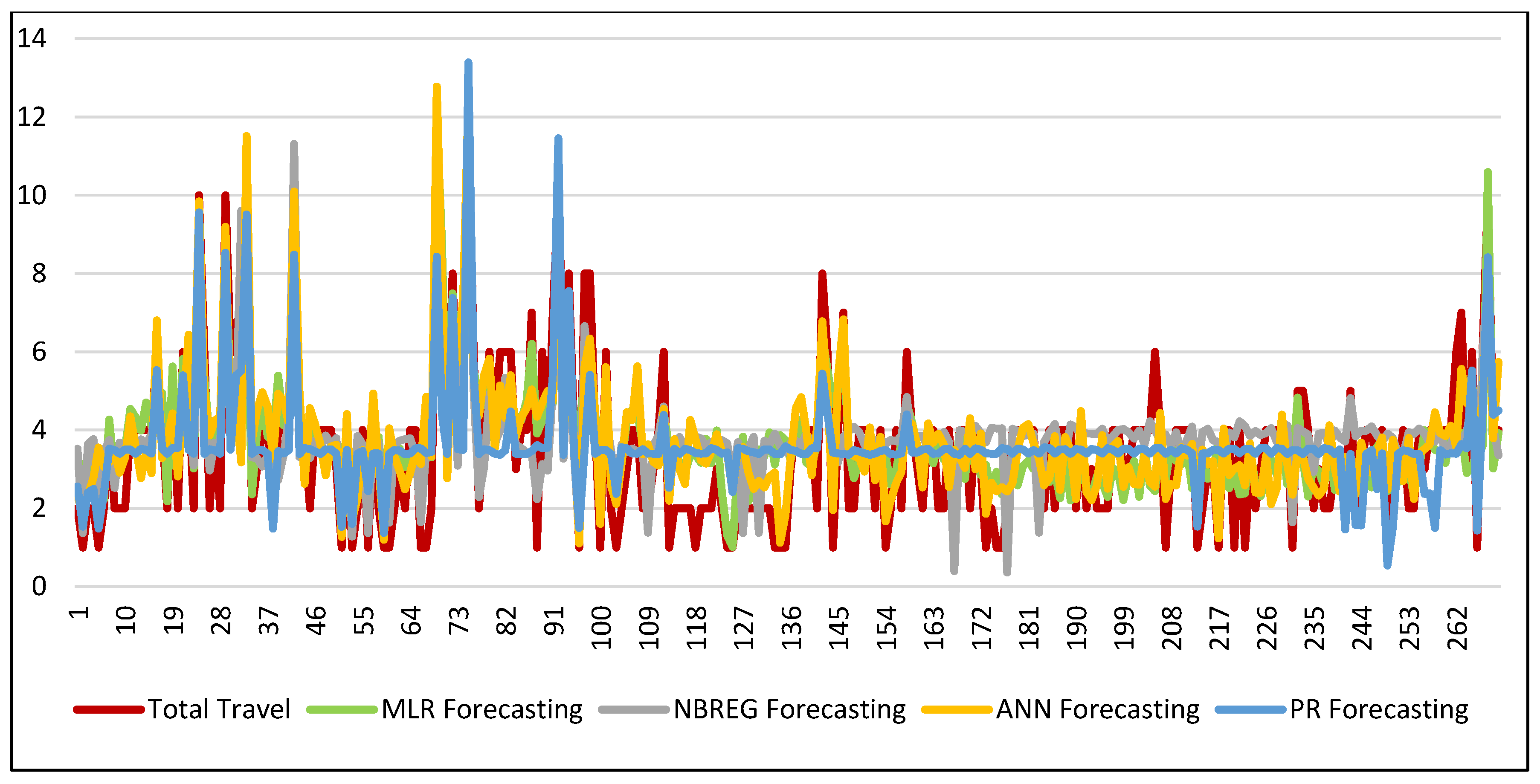
Figure 3 shows the comparison of models developed using MLR, PR, NBREG, and ANN with travel data. Accordingly, ANN was considered the most effective method, as it provided the most accurate forecast of total travel.

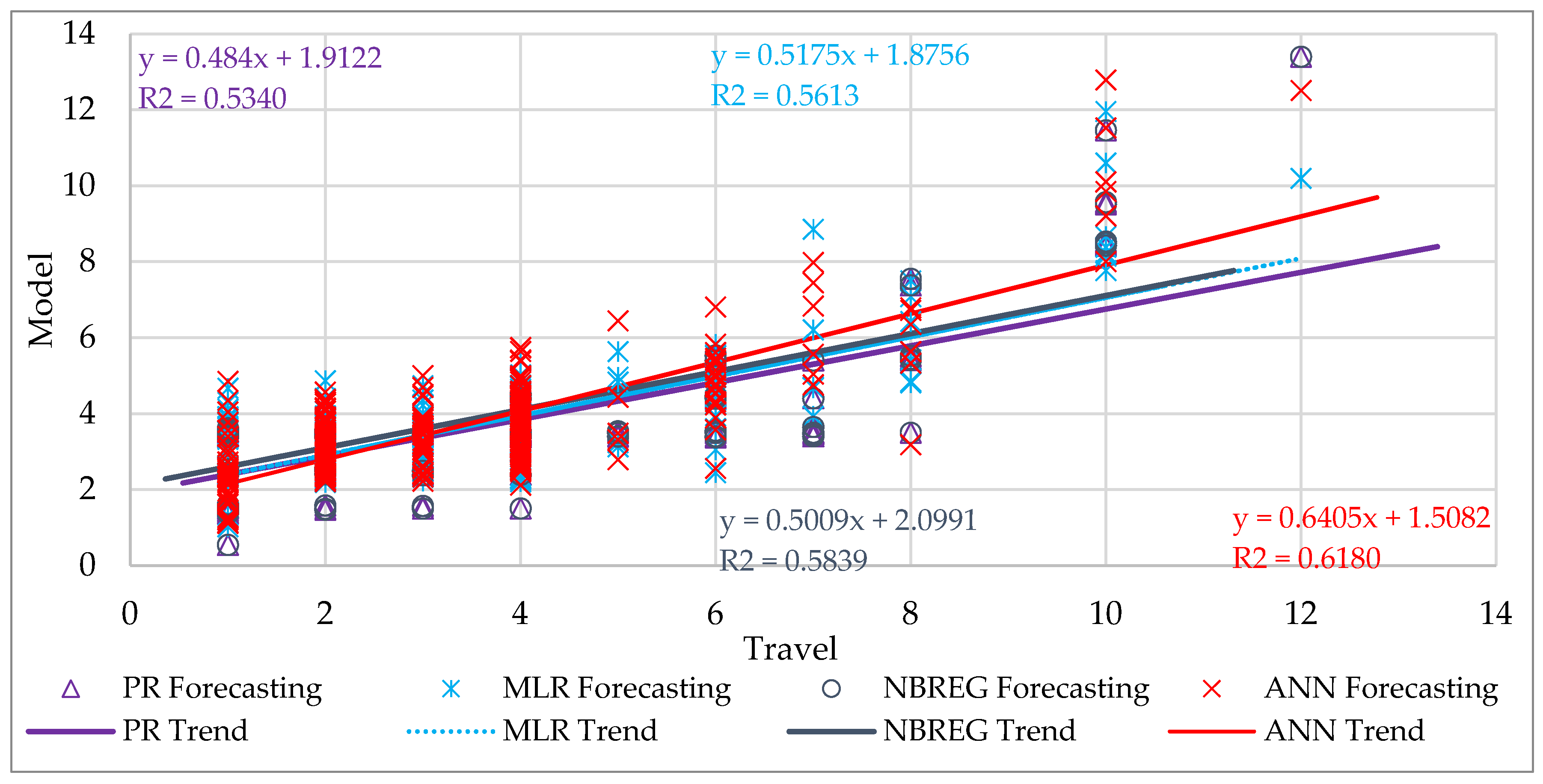
Figure 4 presents the fit graph comparing total household travel with the estimation results obtained from MLR, ANN, PR, and NBREG models. All methods show a consistent pattern in replicating the observed data. Among them, ANN achieved the highest R² (0.618), followed by NBREG (0.5839), MLR (0.5613), and PR (0.5340). ANN and NBREG offer better performance in estimating total household travel compared to the other models.

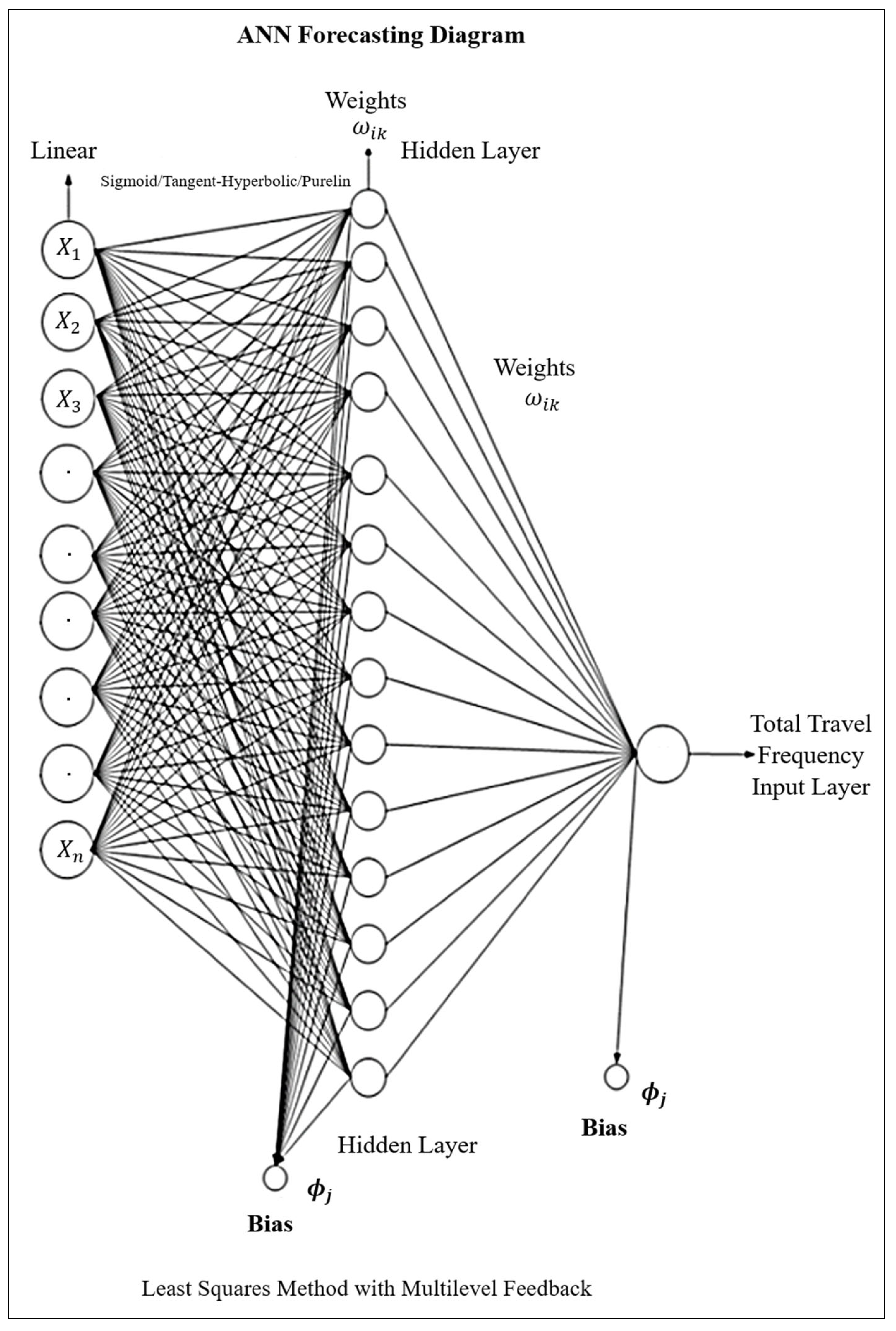
Figure 5 illustrates the neural network architecture employed for the estimation of total household travel using an ANN algorithm. The ANN model was constructed with three hidden layers, each consisting of 13 neurons. The training function used was trainbr (Bayesian Regularization), and the transfer functions applied across the layers were Tansig and Purelin, respectively. The model was trained for 500 iterations (epochs). To evaluate and compare model performance, R², MSE, and the AIC were used as key indicators. Based on the fit and scatter plots, the ANN model demonstrated statistically superior performance compared to other methods. The results showed MSE = 0.003, AIC = −265.15, and R² = 0.62, confirming the ANN as the most appropriate model for predicting total household travel.

Figure 6 presents the NBREG–MLR and PR–ANN graphs, offering a three-dimensional visualization of the interactions between different model outputs used to estimate total travel based on household survey data. The first surface graph illustrates the relationship between NBREG and MLR predictions. The curvature and color distribution across the surface reveal how NBREG estimates vary in relation to LR outputs and how these variations influence total travel. The visible slopes and fluctuations suggest that the relationship between these models is not consistently linear, with distinct peaks and deviations observed throughout the prediction space. The second surface graph displays the interaction between PR and ANN. This surface is smoother and more continuous in structure, indicating a more gradual variation. Notably, areas where both PR and ANN values are high are associated with significantly increased total travel estimates. The color transitions in these regions clearly demonstrate the strong influence of simultaneous increases in both models on travel prediction.

4.1.2. Comparison of Statistical Models of Total Travel from Dormitory Students Surveys

To model the total travel of dormitory students, four methods were applied: MLR, PR, NBREG, and ANN. In all models, the dependent variable is the total travel per student, while the independent variables reflect various socio-economic and demographic characteristics. Definitions of the variables used in Equations (7)–(9) are presented below.

Y: Total travel (dependent variable).

X: Independent variables, where each X_i is defined as follows:

X₁: Age (in years);

X₂: Gender (1: male, 2: female);

X₃: Education level (1: university, 2: postgraduate);

X₄: Employment status (1: employed, 2: unemployed);

X₅: Car ownership (1: yes, 2: no);

X₆: Driver’s license ownership (1: yes, 2: no);

X₇: Monthly income (1: TRY 0–500, 2: TRY 501–2500, 3: TRY 2501–5000, 4: TRY 5001 and above);

X₈: Monthly expense (1: TRY 0–500, 2: TRY 501–2500, 3: TRY 2501–5000, 4: TRY 5001 and above;

X₉: Mode of transportation (1: walking, 2: private car, 3: bus, 4: bicycle, 5: other).

Multiple Linear Regression

Equation (7) models total travel as a function of various dormitory-student-related factors using MLR.

$$\begin{gathered} \mathrm{Y}=2.501+0.005 \ast {\mathrm{X}}_1-0.039 \ast {\mathrm{X}}_2-0.083 \ast {\mathrm{X}}_3+0.062 \ast {\mathrm{X}}_4-0.05 \ast {\mathrm{X}}_5 \\ \hspace{1em}\hspace{1em}-0.005 \ast {\mathrm{X}}_6+0.032 \ast {\mathrm{X}}_7-0.051 \ast {\mathrm{X}}_8-0.066 \ast {\mathrm{X}}_9 \end{gathered}$$

(7)

In regard to the MLR model, the household’s education level is the factor that boosts travel. Aside from that, the gender and employment level of the household members influence travel the most. In short, school and work are the factors that cause travel. The square meters of home housing, parking lot ownership, and housing style are the most effective factors in reducing travel.

Poisson Regression

Equation (8) presents a PR model for total travel, where the intercept value (0.663) indicates the expected level of travel when all predictors are set to zero.

$$\begin{gathered} \mathrm{Y}=0.663+0.003 \ast {\mathrm{X}}_1-0.066 \ast {\mathrm{X}}_2-0.0294 \ast {\mathrm{X}}_3+0.026 \ast {\mathrm{X}}_4+0.033 \ast {\mathrm{X}}_5 \\ \hspace{1em}\hspace{1em}+0.012 \ast {\mathrm{X}}_6+0.024 \ast {\mathrm{X}}_7-0.042 \ast {\mathrm{X}}_8+0.006 \ast {\mathrm{X}}_9 \end{gathered}$$

(8)

Negative Binomial Regression

Equation (9) applies NBREG to model total travel among dormitory students, based on various individual characteristics reflecting their socio-demographic profiles.

$$\begin{gathered} \mathrm{Y}=0.673+0.002 \ast {\mathrm{X}}_1-0.05 \ast {\mathrm{X}}_2-0.01294 \ast {\mathrm{X}}_3+0.0026 \ast {\mathrm{X}}_4+0.044 \ast {\mathrm{X}}_5 \\ \hspace{1em}\hspace{1em}+0.066 \ast {\mathrm{X}}_6+0.015 \ast {\mathrm{X}}_7-0.062 \ast {\mathrm{X}}_8+0.009 \ast {\mathrm{X}}_9 \end{gathered}$$

(9)

In accordance with NBREG modeling, age, employment position, and car ownership are the most important factors in increasing total dormitory travel. In other words, the older, employed, and car-owning members of the dormitory population tend to travel more frequently, and as the average age, employment status, and automobile ownership rise, so will total travel. Gender, education level, and expense status are all factors that contribute to less travel.

Figure 7 compares the total travel calculated from dormitory population surveys using the MLR, PR, NBREG, and ANN estimation models. Given that graph, MLR is the best approach for estimating total travel.

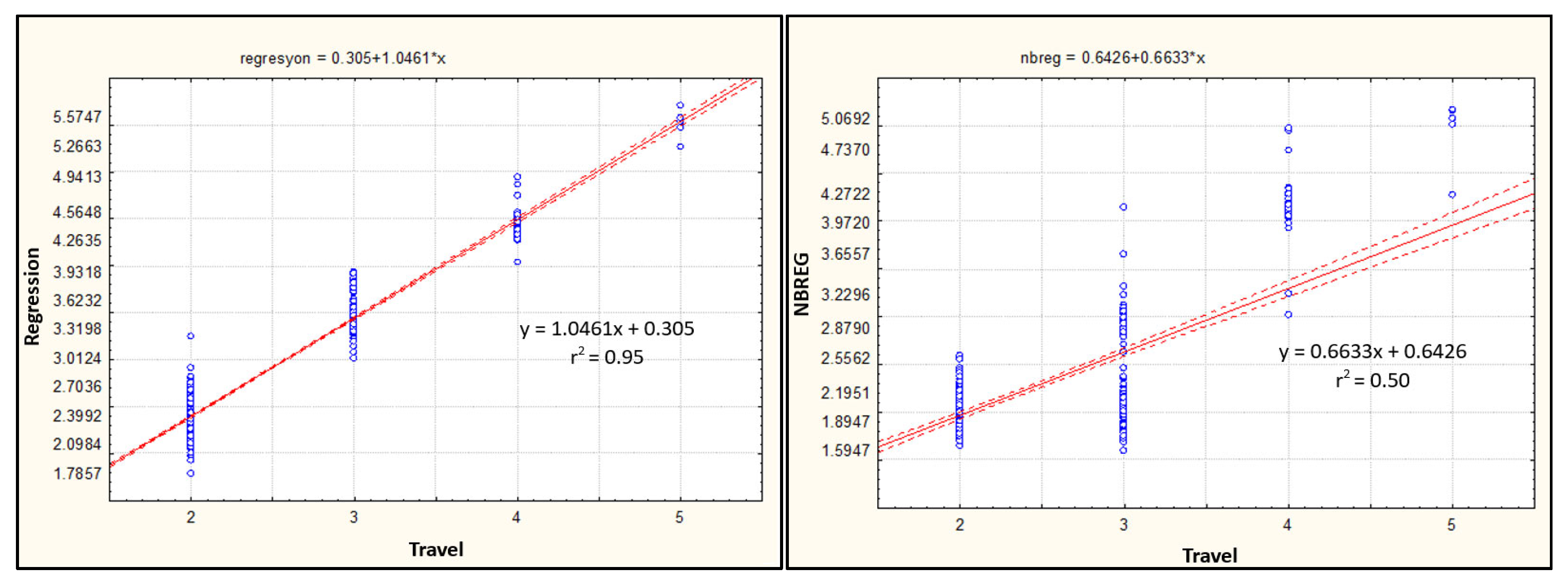
Figure 8 presents the fit graph comparing total travel with the estimation results obtained from MLR, ANN, PR, and NBREG models based on dormitory survey data. All the models demonstrate a generally consistent pattern in capturing the travel behavior, though the degree of fit varies across methods. Among them, MLR achieved the highest coefficient of determination (R² = 0.9538), indicating a very strong linear relationship with the observed travel data. This is followed by ANN (R² = 0.6900), PR (R² = 0.4616), and NBREG (R² = 0.5009). The trend lines also suggest that MLR and ANN provide better alignment with actual travel values compared to PR and NBREG. Overall, the results highlight the superior estimation capability of MLR in this dataset, with ANN also offering promising performance.

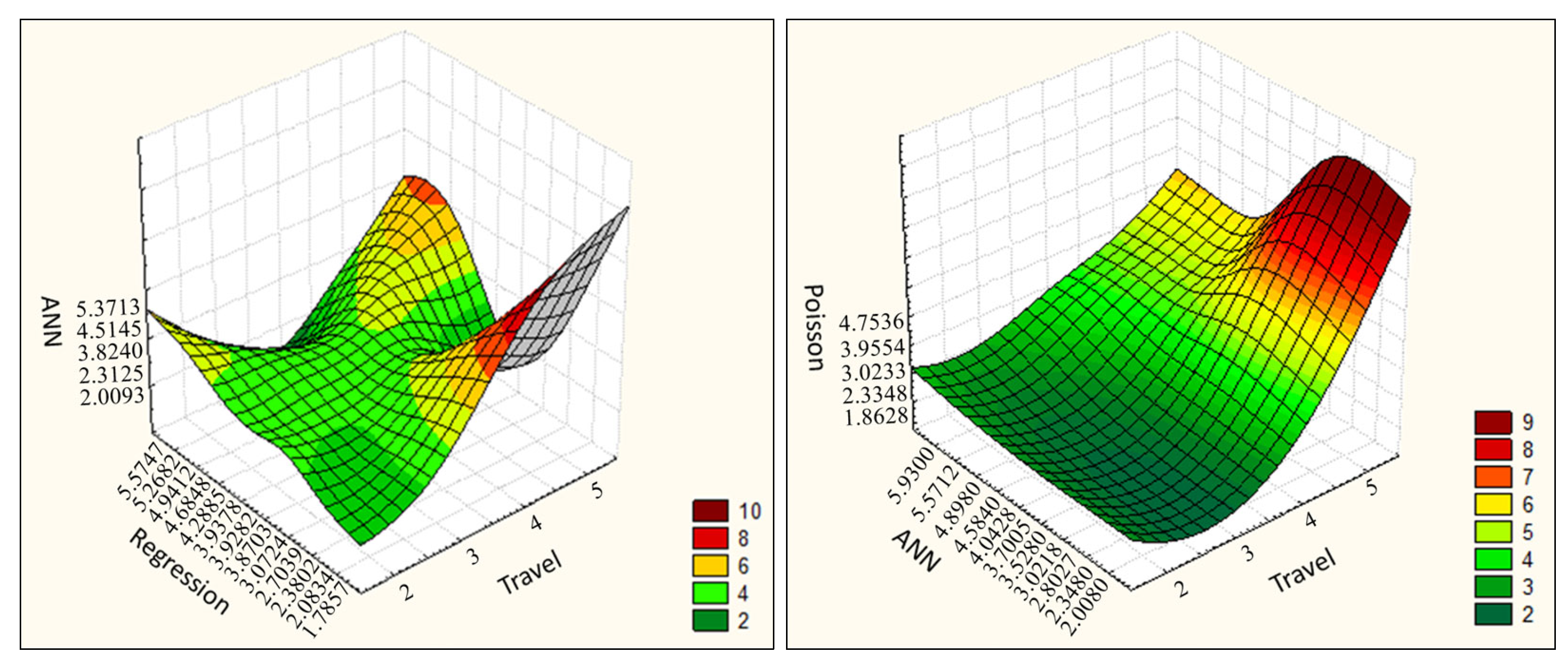
Figure 9 presents the ANN–MLR and PR–ANN graphs, offering a 3D visualization of the interactions between different model outputs used to estimate total travel among dormitory students. The first surface graph shows the relationship between ANN and MLR. The curvature and color distribution reflect how ANN predictions vary with respect to MLR estimates and how these differences influence total travel values. Red and yellow areas indicate higher travel estimates, while green areas represent lower values. This reveals that the relationship between the models is not consistently linear, with visible peaks and deviations.

The second surface graph illustrates the interaction between ANN and PR. This surface is smoother, and regions with high values from both models correspond to a significantly higher total travel. The color transitions demonstrate how simultaneous increases in ANN and PR outputs affect travel estimation.

4.1.3. Macro-Simulation

In household surveys conducted in Erzincan, 57.79% of households own private cars. While 22.10% of people drive, 60.10% use public transportation. Erzincan province’s public transportation system is limited to bus services. These can carry up to 50 passengers. According to the surveys, 20.50% of those who used public transit said the service was very bad, while 36.70% said it was satisfactory. The percentage of respondents who said it was good remained at 1.70%. And 41.50% of respondents blamed exorbitant transportation fees, while 25.20% accused crowding. While 8.40% complained about the distance between stations, 12.10% claimed the routes were not appropriate. There are 13 public transit lines that operate from 6:00 a.m. to 22:30 p.m.; after 23:00, buses operating on the night line provide service.

To examine the current public transportation system, time-based assignments were made during the morning peak hours of 07:30 and 08:30. Connectors for highway and public transportation between zones, as well as public transportation stops and start–destination matrices, were designed for this purpose. The timetables and routes of current lines were collected from Erzincan Municipality, and demand matrices for 26 zones were entered into the VISUM application. Figure 10 shows the 26 zones established for Erzincan province.

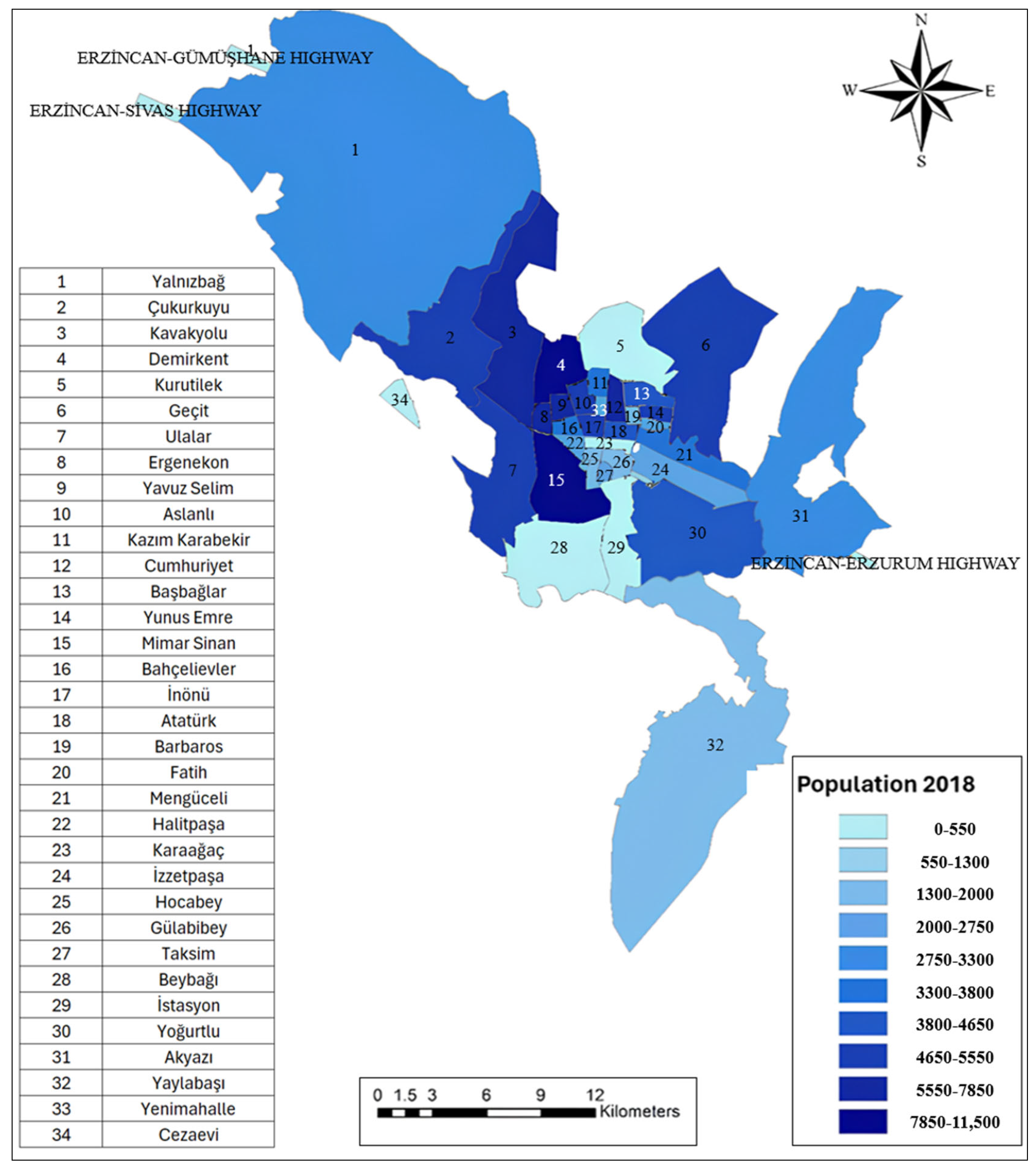
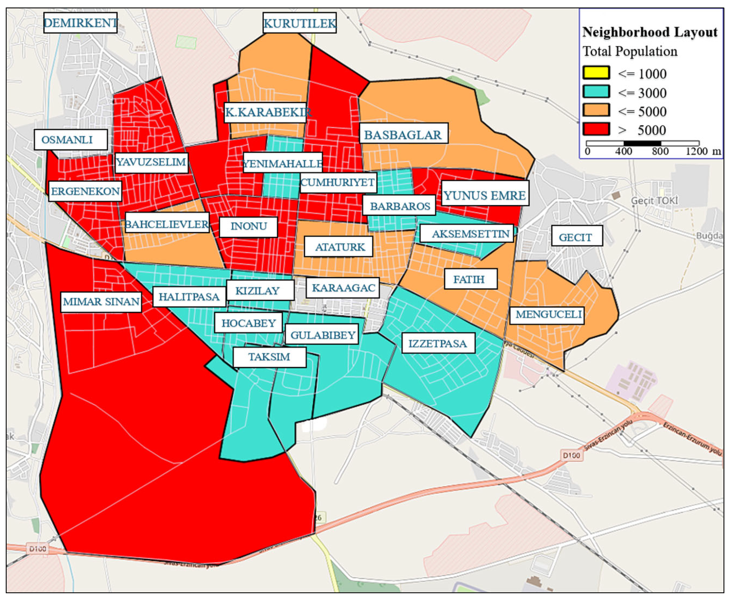
The current settlement of the neighborhoods in the city center depends on their population, as shown in Figure 11. Neighborhoods with a population greater than 5000 are shown in red, while those less than 1000 are shown in yellow. Others are shown in intermediate colors.

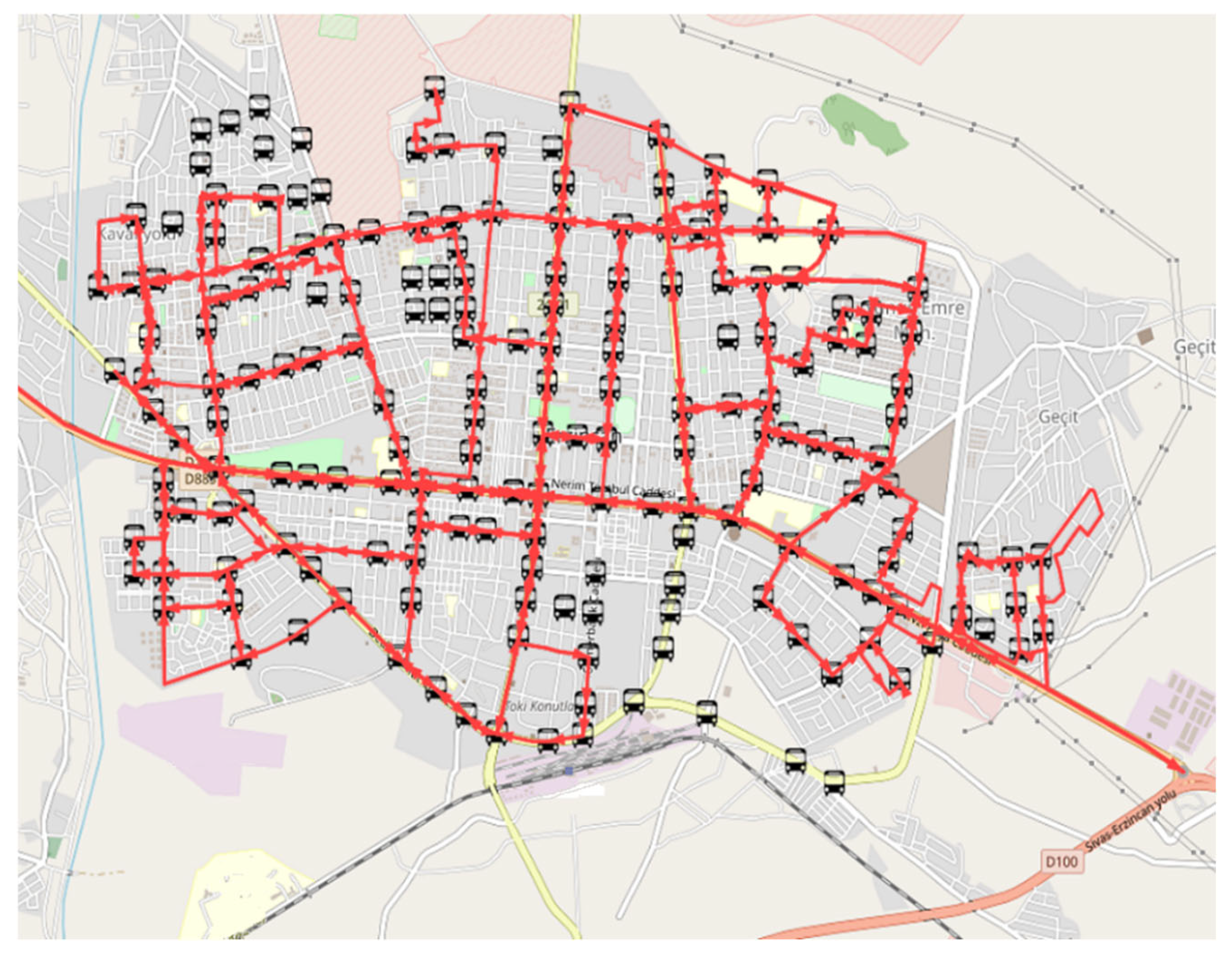
Figure 12 depicts the departure times and stop locations of currently operational urban bus lines in Erzincan, which were obtained from the Erzincan Municipality and modeled in VISUM. The red lines represent the bus routes, while the bus icons indicate the designated bus stops used in the urban public transportation network.

Table 4. Travel times for automobile trips based on the PR model.

No	Origin	Destination	Duration (min)	No	Origin	Destination	Duration (min)
1	Yalnızbağ	İzzetpaşa	22.77	16	Yalnızbağ	Gülabibey	19.84
2	Yalnızbağ	Yunus Emre	22.32	17	Basbağlar	Yalnızbağ	19.65
3	Yalnızbağ	Akşemsettin	21.94	18	Yalnızbağ	Hocabey	19.54
4	Yalnızbağ	Mengüceli	21.88	19	Yalnızbağ	K. Karabekir	19.51
5	İzzetpaşa	Yalnızbağ	21.86	20	Cumhuriyet	Yalnızbağ	19.46
6	Yunus emre	Yalnızbağ	21.49	21	Yalnızbağ	Atatürk	19.21
7	Yalnızbağ	Barbaros	21.48	22	Yenimahalle	Yalnızbağ	19.18
8	Yalnızbağ	Fatih	21.42	23	Yalnızbağ	Karaağaç	19.17
9	Akşemsettin	Yalnızbağ	21.09	24	Gülabibey	Yalnızbağ	18.99
10	Mengüceli	Yalnızbağ	20.96	25	Hocabey	Yalnızbağ	18.70
11	Barbaros	Yalnızbağ	20.59	26	K. Karabekir	Yalnızbağ	18.68
12	Fatih	Yalnızbağ	20.52	27	Yalnızbağ	Çarşı	18.58
13	Yalnızbağ	Basbağlar	20.52	28	Atatürk	Yalnızbağ	18.34
14	Yalnızbağ	Cumhuriyet	20.31	29	Karaağaç	Yalnızbağ	18.31
15	Yalnızbağ	Yenimahalle	20.04	30	Yalnızbağ	Aslanlı	18.30

presents the 30 automobile trips with the longest travel times out of a total of 676 trips distributed using the PR model. Accordingly, the trip with the longest travel time among the trips made by automobile was from Yalnızbağ Neighborhood to İzzetpaşa Neighborhood, and it took approximately 23 min.

Table 5. Travel times for bus trips based on the PR model.

No	Origin	Destination	Duration (min)	No	Origin	Destination	Duration (min)
1	Mengüceli	Yalnızbağ	40.75	16	İnönü	Yalnızbağ	27.84
2	Çarsı	Yalnızbağ	39.87	17	Yalnızbağ	Mengüceli	27.69
3	Taksim	Yalnızbağ	37.11	18	Yenimahalle	Yalnızbağ	25.16
4	Yavuz Selim	Yalnızbağ	34.55	19	Çarşı	Fatih	24.54
5	Aslanlı	Yalnızbağ	33.12	20	Yalnızbağ	Yavuz Selim	24.61
6	Fatih	Yalnızbağ	33.85	21	Yalnızbağ	Fatih	24.68
7	İzzetpaşa	Yalnızbağ	32.16	22	Yalnızbağ	Aslanlı	24.26
8	Ergenekon	Yalnızbağ	31.15	23	Yalnızbağ	İzzetpaşa	24.48
9	Bahçelievler	Yalnızbağ	30.64	24	Yalnızbağ	Osmanlı	23.32
10	Barbaros	Yalnızbağ	30.26	25	Basbağlar	Yalnızbağ	23.17
11	Yalnızbağ	Çarşı	29.75	26	Yunus emre	Yalnızbağ	23.55
12	Gülabibey	Yalnızbağ	29.49	27	Kızılay	Yalnızbağ	23.34
13	Hocabey	Yalnızbağ	28.38	28	Çarşı	K. Karabekir	23.95
14	Cumhuriyet	Yalnızbağ	28.16	29	Çarşı	Cumhuriyet	23.16
15	Osmanlı	Yalnızbağ	27.19	30	Akşemsettin	Yalnızbağ	22.16

shows the 30 bus journeys with the longest durations out of 676 total trips allocated using the PR model. The bus trip from Mengüceli Neighborhood to Yalnızbağ Neighborhood was the longest, lasting around 41 min.

Using the NBREG model, the travel times of 676 automobile trips were analyzed, among which 30 with the longest durations are presented in

Table 6. Travel times of automobile trips depending on the NBREG model.

No	Origin	Destination	Duration (min)	No	Origin	Destination	Duration (min)
1	Yalnızbağ	Izzetpaşa	23.12	16	Yalnızbağ	Gülabibey	20.17
2	Yalnızbağ	Yunus emre	22.67	17	Basbağlar	Yalnızbağ	19.91
3	Yalnızbağ	Akşemsettin	22.28	18	Yalnızbağ	Hocabey	19.88
4	Yalnızbağ	Mengüceli	22.22	19	Yalnızbağ	K. Karabekir	19.83
5	İzzetpaşa	Yalnızbağ	22.00	20	Cumhuriyet	Yalnızbağ	19.63
6	Yunus emre	Yalnızbağ	21.81	21	Yalnızbağ	Atatürk	19.54
7	Yalnızbağ	Barbaros	21.76	22	Yenimahalle	Yalnızbağ	19.49
8	Yalnızbağ	Fatih	21.63	23	Yalnızbağ	Karaağaç	19.32
9	Akşemsettin	Yalnızbağ	21.23	24	Gülabibey	Yalnızbağ	19.13
10	Mengüceli	Yalnızbağ	21.09	25	Hocabey	Yalnızbağ	18.94
11	Barbaros	Yalnızbağ	20.93	26	K. Karabekir	Yalnızbağ	18.85
12	Fatih	Yalnızbağ	20.74	27	Yalnızbağ	Çarşı	18.84
13	Yalnızbağ	Basbağlar	20.71	28	Atatürk	Yalnızbağ	18.67
14	Yalnızbağ	Cumhuriyet	20.65	29	Karaağaç	Yalnızbağ	18.48
15	Yalnızbağ	Yenimahalle	20.37	30	Yalnızbağ	Aslanlı	18.47

. The longest travel time was from Yanlızbağ Neighborhood to İzzetpaşa Neighborhood, taking around 23 min.

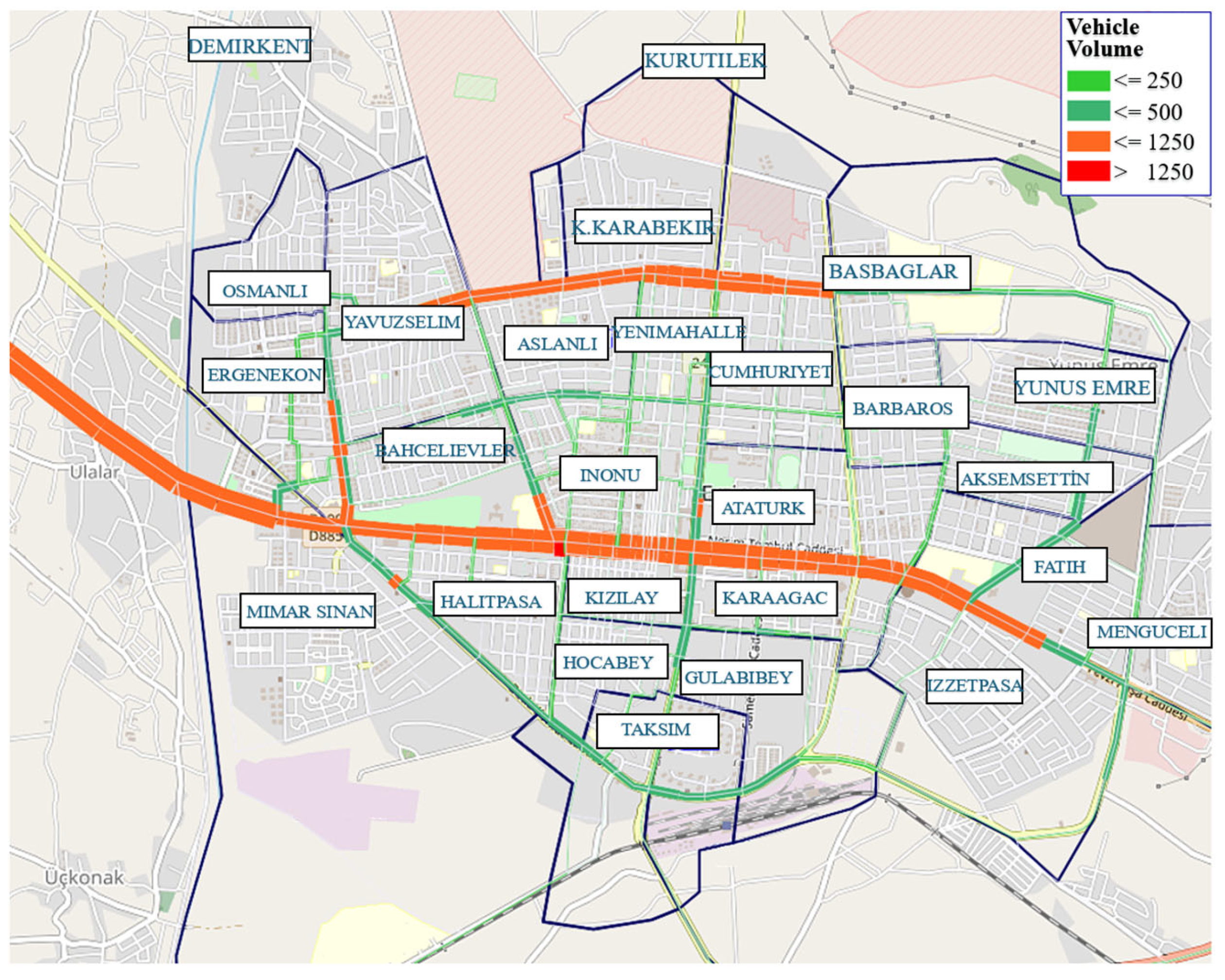
The service levels according to the appointments made according to the PR model are given in Figure 13. Accordingly, while the service levels are D and E on Halit Paşa Street, Milli Egemenlik Street and Ergenekon Avenue provide service levels of C and D. On other roads, the service level is generally B, although it varies from place to place.

Based on the NBREG model, the service levels on Halit Paşa Street are D and E, whilst Milli Egemenlik Street and Ergenekon Avenue provide service at the B and C levels. Other roads have a general service level of B, albeit this varies by location.

The bus trip with the longest duration among the 676 total bus rides dispersed using the MLR model is from Mengüceli Neighborhood to Yalnızbağ Neighborhood, taking around 41 min. From the appointments made using the MLR model, the service levels on Halit Paşa Street are E and F, whereas Milli Egemenlik Street and Ergenekon Avenue give D and E service levels. On other roads, service levels are B and C.

Among the 676 bus trips distributed using the ANN model, the trip with the longest travel time is from Mengüceli Neighborhood to Yalnızbağ Neighborhood and lasts approximately 41 min. In response to the ANN model’s allocations, Halit Paşa Street normally has service levels of D and E, with one intersection having service level F. Meanwhile, Milli Egemenlik Street and Ergenekon Avenue provide service levels C and D. Other roads have a general service level of B, albeit this varies by location.

4.2. Discussion

The findings of this study demonstrate that the fundamental socio-demographic factors influencing travel behavior among households and dormitory students in Erzincan can be effectively modeled. Four modeling techniques, MLR, PR, NBREG, and ANN, were comparatively tested, and the most appropriate prediction method was identified for each population group. For household data, the ANN model achieved the highest accuracy, whereas for dormitory students, MLR proved to be the most effective. In the household travel estimation, education level, gender of the household head, and employment status emerged as the most significant variables that increase travel. These findings highlight the critical role of work and school-related mandatory trips in overall trip generation. Moreover, the PR and NBREG models indicated that household size, total floor area, and driver’s license ownership were also positively associated with travel frequency. Conversely, factors such as homeownership, availability of parking spaces, and housing type were found to reduce travel propensity, suggesting that spatial comfort may lessen the need for frequent travel.

In the dormitory student model, factors that enhance individual mobility capacity, such as age, employment status, and car ownership, were positively associated with travel frequency. On the other hand, some variables, including education level, spending capacity, and gender, were observed to reduce travel. This may indicate that postgraduate students engage in fewer off-campus activities or maintain more sedentary lifestyles. Additionally, the reduced travel among students with lower expenditure levels could be interpreted as suppressed demand, reflecting unmet transportation needs.

These findings offer important strategic implications for urban planning. Given that neighborhoods with higher concentrations of educated, employed, and larger families exhibit more intense travel demand, public transport supply in these areas should be expanded. In regions with widespread vehicle ownership, the promotion of alternative transport modes should be prioritized. Furthermore, VISUM-based simulations revealed low service levels along major corridors such as Halit Paşa and Ergenekon Streets, emphasizing the need for prioritizing infrastructure investments in these areas. The reduced travel associated with homeownership and larger housing spaces may imply that spatial needs are being met locally, indicating the value of promoting walkable and mixed-use urban developments. By integrating the model outputs into transport simulation tools, planners can assess the future impacts of scenarios such as new campus openings or housing developments in advance. This study not only evaluates the predictive performance of various models but also provides concrete guidance on how they can inform data-driven and sustainable urban transport planning.

4.3. Comparison with Other Studies

In the study by Varga et al. [25], a mesoscopic simulation methodology was employed, which, unlike our study, incorporated vehicle dynamics into large-scale traffic planning. This approach goes beyond merely determining overall traffic demand and route assignment, enabling a more detailed analysis of traffic flow. As a result, dynamic parameters such as congestion and delay can be effectively examined.

Ma et al. [45] proposed a methodology that combines the centroid triangular white weight function with the entropy–AHP method for evaluating urban green transportation planning. Considering the limitations of our study, incorporating alternative decision-making applications in future research could be a valuable and developmental approach.

Shaikh et al. [7] proposed a methodology based on the integration of artificial intelligence (AI), blockchain, and dynamic computation techniques to improve traffic management through traffic flow analysis. Unlike our work in the scope of traffic planning, their approach focused on dynamic traffic improvements.

In their study, Liang et al. [10] focused on bicycle travel production. Starting with a small-scale pilot system, new stations were gradually added. In this process, the estimated demand for new stations has been a crucial determining factor. The Spatial-MGAT model, which takes spatial relationships into account, is proposed as a model. Similarly to our study, travel time calculations for public transportation and individual vehicle analysis are not among the goals of this work. However, in future studies, the inclusion of micro-mobility vehicles, such as bicycles and scooters, in urban transportation planning could be considered. Our study has certain limitations in terms of micro-mobility.

Wang et al. [17] introduced a new large language model in the field of transportation, called TransGPT. The model has demonstrated superior performance in various domains, including traffic engineering, urban planning, traffic management, and driver examinations. The study showcased the model’s applicability in areas such as traffic flow prediction and the generation of synthetic traffic scenarios. In future studies, it may be possible to develop a language model specifically aimed at urban transportation planning, aligned with the context of our work, which could significantly facilitate the planning process.

Dikshit et al. [5] presented a methodology that utilizes AI and machine learning techniques to predict traffic flow, optimize traffic signal timings, and guide autonomous vehicles. Unlike our study, their work included autonomous vehicles within its scope. A future transportation planning framework that also incorporates autonomous vehicles and allows for dynamic management could be considered.

Dabiri and Heaslip [51] predicted transportation modes using GPS data. Access to information on transportation modes, one of the fundamental stages of transportation planning, is crucial for enhancing planning effectiveness. By leveraging Convolutional Neural Networks (CNNs), high-level predictions can be made directly from raw GPS data, which has the potential to significantly improve the efficiency of transportation planning processes. Therefore, this approach is recommended for use in transportation planning.

Zrigui et al. [26] aimed to achieve real-time traffic planning to reduce global greenhouse gas emissions originating from transportation. Since it is not possible to effectively reduce such emissions without addressing negative transportation outcomes like congestion and delays, a comprehensive optimization of the transport system can be achieved in this direction. Incorporating real-time predictions of transportation modes and travel times into such studies could offer an inspiring direction for future research. This study, briefly referred to as “transportation planning”, offers a comprehensive approach due to its inclusion of real-time improvements.

Mecheva et al. [24] modeled factors such as drivers’ mood, fatigue, and responses to distracting stimuli in traffic simulations. They developed a method to identify the most representative traffic simulation parameters that reflect driver behavior accurately. This method aims to select the optimal combination by using different distance models and routing algorithms. In their study, over 7000 simulations were conducted using SUMO (Simulator for Urban Mobility) and Python, which revealed that the most suitable model for traffic in Plovdiv was the Krauss following distance model combined with the Contraction Hierarchies routing algorithm. In the context of our work, future studies could combine both macroscopic and mesoscopic models. Additionally, mesoscopic simulations, calibrated with driver behavior, could provide a broader and more comprehensive framework.

5. Conclusions

This study utilized two distinct survey types alongside four robust statistical techniques to establish a comprehensive framework for transportation planning. The reliability of the survey findings was thoroughly assessed, and models derived from MLR, ANN, PR, and NBREG were critically compared. Trip generation was estimated based on data from both household and dormitory surveys, integrating key demographic and socioeconomic variables, along with transportation planning zones. Given the significant capital expenditures associated with transportation infrastructure, reducing investment costs in small-scale urban environments is vital for the development of efficient transportation systems.

One of the key contributions of this study is the comparison of various statistical models that can be used in transportation planning. The analyses conducted with household and dormitory survey data lay a strong foundation for more accurate and efficient travel demand predictions in transportation planning. Each of the models used in the study demonstrated varying levels of success on different datasets. These findings provide valuable insights for selecting the most suitable model for transportation planning.

The methodologies employed for household trip modeling were rigorously evaluated through the coefficient of determination (R²), MSE, and AIC, which served as discriminative factors in model selection. The ANN approach demonstrated the highest statistical fit, with MSE = 0.003, AIC = −265.148, and R² = 0.62, indicating its robustness in predicting trip generation for household data. The success of ANN can be attributed to its ability to learn complex relationships within the data. The results from the household surveys indicate that this model can be used to make more efficient predictions in transportation planning. On the other hand, for dormitory-based trips, linear MLR emerged as the most suitable model, with MSE = 0.006, AIC = −65.148, and R² = 0.95, showing superior performance in capturing the travel behavior of student populations. This result suggests that dormitory data contain simpler and more linear relationships, making MLR a more suitable model for such data. Additionally, PR and NBREG models produced significant results for predicting vehicle travel times. Each of these models showed varying levels of success in determining travel times for vehicles.

When comparing the LR, PR, NBR, and ANN models, the estimated automobile travel times to determine the shortest route were 29.53, 22.77, 23.13, and 25.93 min, respectively. Among these, the PR produced the optimal travel distribution. Furthermore, the travel times for current public transportation routes, based on these travel distributions, were found to be approximately 40.78, 40.75, 40.48, and 40.43 min for MLR, PR, NBR, and ANN, respectively. As no deviations from existing public transportation routes were considered, the travel times for all models remained fairly comparable, underscoring that all models are equally viable for evaluating public transit efficiency.

Moreover, PTV VISUM was employed as a macro-simulation tool, and the impact of the travel distributions generated by the MLR, PR, NBR, and ANN models on the current transportation conditions was analyzed. It is important to note that no improvement scenarios—such as changes in land use, road network additions, or alterations to public transportation routes—were proposed beyond existing infrastructure. These enhancements may be explored in future studies. The data entered into PTV VISUM therefore provide a comprehensive foundation for numerous subsequent studies, facilitating the development of more refined urban transportation planning models.

This study’s limitations include the absence of improvement scenarios for existing transportation infrastructure. The analysis in this study was based solely on current travel distributions and existing transportation systems. Future research could develop more comprehensive scenarios by examining the effects of new road additions, changes to public transport lines, or alterations in land use. Another limitation is that the surveys used were limited to a specific geographic area. In this study, the city of Erzincan was chosen as the sample, and the results may be limited to this region. However, the selection of Erzincan, a medium-sized city with data constraints, also makes the study unique.

Building on the findings of this study, future research may concentrate on evaluating potential enhancements to urban transportation infrastructure under various planning scenarios. This may include assessing the implications of modifications such as expanding the road network, introducing new links, relocating signalized intersections, or adjusting public transport routes. The broader, long-term effects of such interventions on system performance and network efficiency can be further examined through advanced transportation simulation tools. In addition, future research could focus on enhancing model accuracy through the integration of real-time behavioral data and the application of techniques that capture geographic and temporal variation. Convolutional Neural Networks (CNNs), Recurrent Neural Networks (RNNs), or hybrid approaches such as ensemble learning or Bayesian-optimized neural networks may improve the models’ ability to learn complex, non-linear patterns in travel data. Integrating these predictive models with simulation tools in real time may further enhance adaptive and responsive transportation planning. Moreover, adapting predictive models to evaluate social equity and environmental sustainability could contribute to the development of more inclusive and responsible urban transportation strategies.