Article

Application of Proper Orthogonal Decomposition to Elucidate Spatial and Temporal Correlations in Air Pollution Across the City of Liverpool, UK

by
Cammy Acosta Ramírez
and
Jonathan E. Higham
*
School of Environmental Sciences, University of Liverpool, Roxby Building, Liverpool L69 3BX, UK
*
Author to whom correspondence should be addressed.
Urban Sci. 2025, 9(5), 166; https://doi.org/10.3390/urbansci9050166
Submission received: 29 January 2025 / Revised: 10 April 2025 / Accepted: 15 April 2025 / Published: 13 May 2025

Abstract

:
Understanding the spatiotemporal distribution of air pollution is critical for improving urban air quality. Advances in wireless sensor networks have made it possible to monitor air pollution across cities at higher spatiotemporal resolutions. The new spatial coverage allows the novel implementation of advanced statistical methods to detect spatially important, coherent patterns in environmental flows. In this study, we apply proper orthogonal decomposition to a spatial distribution derived from 34 particulate matter sensors, which collected data over 250 days across the Liverpool City Region in England, to identify a set of spatially orthogonal modes. The dominant mode exhibits a daily periodicity in the increases of particulate matter, with higher increases in residential areas interpreted as changes driven by daily commutes. The second mode highlights seasonal changes, and the third mode alludes to pollution transportation with simultaneous increases and decreases. In contrast with traditional time series and spatial analyses, proper orthogonal decomposition enables the elucidation of patterns that otherwise might remain hidden. Our findings highlight the benefits of urban wireless sensor networks and demonstrate the applicability of proper orthogonal decomposition in studying the movements of polluted areas and their correlations with meteorological variables and anthropogenic factors.

1. Introduction

Poor air quality is considered one of the most important public health concerns of this century. In 2019, the World Health Organization (WHO) estimated that outdoor air pollution caused 4.2 million premature deaths worldwide [1]. Air pollutants have been linked to a variety of health effects, including respiratory diseases, as well as coronary and neurological disorders [2,3,4,5,6]. Particulate matter (PM), nitrogen dioxide (NOx), sulfur dioxide (SO2), and ozone (O3) are among the pollutants with the strongest evidence for public health concern.
The combustion of fossil fuels and industrial activities are recognized as major sources of air pollution, particularly in densely populated urban areas. In the United Kingdom, advances in technology and stricter regulations on mobile and stationary sources of air pollution have led to air quality improvements over the past three decades, particularly in reducing NOx and SO2 [7]. However, diverse pollutants with a variety of complex sources, such as PM, present ongoing challenges in monitoring and establishing goals for air pollution control.
From a public health perspective, exposure to PM has been widely documented as a significant risk factor for negative health outcomes, including heart disease, respiratory disorders, cognitive decline, and metabolic disorders [8,9]. Long-term exposure to PM has been shown to increase inflammation and oxidative stress in the body, leading to an elevated risk of cardiovascular events such as heart attack and stroke [10,11]. Additionally, research has linked PM exposure to a heightened risk of diabetes, obesity, metabolic syndrome, and cognitive impairments such as attention-deficit/hyperactivity disorder (ADHD) and Alzheimer’s disease [12,13,14,15,16,17].
Despite strong evidence linking PM exposure to negative health outcomes, there are still limitations to quantitative aspects of the research that need to be addressed. The major significant challenge is the lack of comprehensive air pollution monitoring, particularly at the city level. Although PM monitoring is a relatively common practice in urban areas, until recently, the majority of air pollution monitoring networks were low-density, capturing one-dimensional (1D) data to describe the complex makeup of urban environments often spanning tens of kilometers [18]. This limited coverage has made it difficult to capture the full spatial and temporal variability of PM in urban areas; without fine grain measurements, it is difficult to make informed decisions to mitigate or reduce air pollution i.e., low-emission zones [19]. To address this limitation, multiple projects have demonstrated the use of high-density wireless sensor networks (WSNs) using semiconductors and optical particle counters for urban air quality monitoring [20,21,22,23,24]. With these networks, it is now possible to obtain a two-dimensional (2D), quasi-3D picture of pollution levels by interpolating data across the time series of sensors (nodes), taking into account localized impacts on air pollution levels over fixed time intervals [25,26].
The shift from 1D to 2D data availability in research is not a new phenomenon, as it has been observed before, particularly in the field of experimental fluid mechanics in the early 1980s. Prior to this time, fluid mechanics research relied heavily on single-point laser and other probe measurements, which provided limited information about fluid flow patterns, particularly in complex fully 3D turbulent flow systems. The advent of image-based techniques such as particle image velocimetry (PIV) allowed researchers to gather more comprehensive and detailed data about fluid flow patterns in a variety of systems [27]. Similarly, the use of WSNs in air quality research allows us to obtain quasi-3D representations of pollution levels across a city, enabling a better understanding of the spatial representation of pollution levels and the identification of spatially coherent or repeating patterns that were previously hidden.
The ability to capture quasi-3D representations of pollution levels also requires the application of statistical methods that can identify urban spatiotemporal patterns and their correlations with meteorological conditions. One such technique that has been successfully used in fluid mechanics is the proper orthogonal decomposition (POD), which allows the detection of coherent structures by analyzing the statistical properties of the flow data [28]. POD decomposes large datasets into spatially orthogonal Eigen-functions (modes), where each mode represents a dominant feature or pattern of variation in the system, providing a basis for the understanding of the organization of a flow [29,30,31,32]. In simpler terms, POD breaks down complex air pollution data into key patterns, like snapshots of how pollution moves and changes across the city. Compared to other dimensionality reduction techniques such as principal component analysis (PCA), dynamic mode decomposition (DMD), or independent component analysis (ICA), POD is particularly well-suited for urban air pollution studies due to its ability to extract spatially orthogonal modes that maximize variance, directly relating to physical structures in environmental flows. While PCA is statistically similar, it lacks the physical interpretability of POD’s spatial modes in fluid-like systems. DMD focuses on dynamic evolution but requires higher temporal resolution data [33], often unavailable in air quality monitoring, whereas ICA assumes statistical independence, which may not hold for correlated pollution patterns. POD’s optimality in capturing dominant variance with fewer modes makes it ideal for identifying coherent pollution structures across Liverpool’s complex urban landscape. For instance, POD has revealed seasonal ice velocity patterns in Greenland glaciers [34] and pollutant dispersion in urban street canyons [35], demonstrating its versatility in environmental applications beyond this study.
POD can be a powerful technique for the detection of elusive coherent structures that populate air pollution patterns, and which could be overlooked by traditional methods of analysis. This has been demonstrated in the analysis of environmental flows in meteorology, oceanography, and glaciology with POD [32,34,35,36,37]. Likewise, recent reviews of the application of all techniques in elucidating patterns for solar flares demonstrated its strong environmental applicability [38,39]. In this paper, we apply POD to understand spatiotemporal patterns of PM pollution data captured by a WSN in the Liverpool City Region in the United Kingdom. Liverpool’s unique geography, characterized by the River Mersey’s influence, varying elevation, and dense urban-industrial mix, poses specific challenges for air quality monitoring, such as localized pollution hotspots and variable dispersion patterns driven by coastal meteorology. POD is employed here to disentangle these complex interactions, leveraging its strength in identifying spatially coherent structures that traditional methods might miss amidst such geographic variability. This paper is structured as follows: First, we describe the WSN and how the data are obtained. Next, we describe the dataset using traditional methods of data analysis. This is followed by the application of POD to decompose the dataset into a set of deterministic spatial functions (modes) and temporal coefficients, which can be used to define and observe complex features. We compare each of these techniques, summarizing our findings in the conclusions section. This novel application of the POD to data obtained from a WSN extends the current arsenal of tools typically used to understand spatial and temporal patterns of air quality across an urban environment.

2. Methods

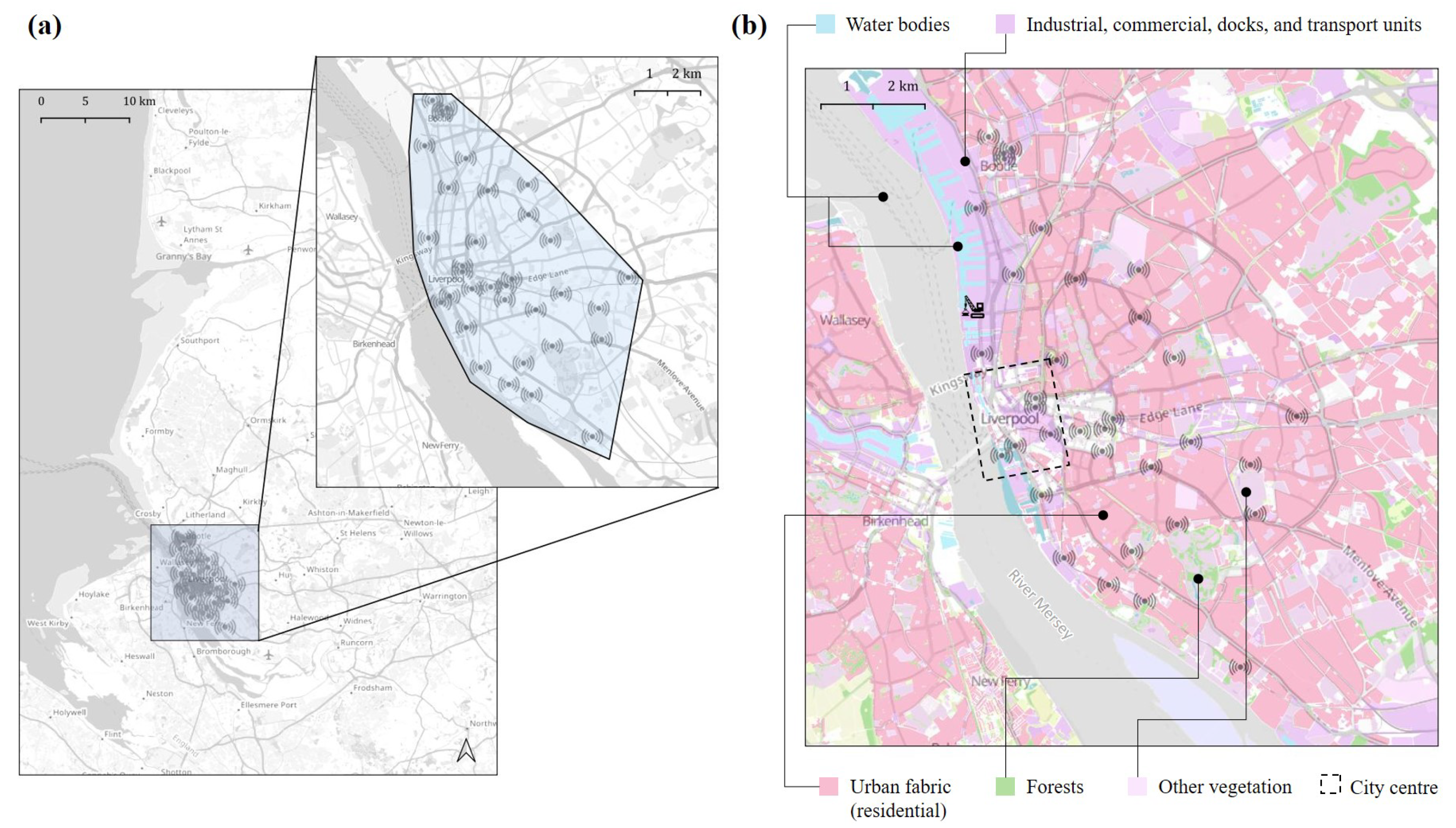
2.1. Study Area and Descriptive Analysis

The Liverpool City Region (LCR) is located in the North West Region in England and has a population of 486,100 people, ranking 34th in population density in England and Wales with 4347 people per square kilometer [40]. One of the most notable features of the LCR is the River Mersey, stretching for 70 miles from Stockport to Liverpool Bay. The climate in this area is defined as Marine West Coast (Cfb) according to Köppen Climate Classification [41]. The elevation in the center of the LCR is 70 m above sea level, and the annual mean average ground temperature is 10.5 °C. In 2011, an equivalent of between 800 to 1040 deaths in the LCR was estimated to be attributable to anthropogenic PM2.5 and NO2 [42]. A task to examine the issue of air quality in the LCR led to the creation of clean air zones, through initiatives such as green infrastructure, pollution mitigation, communication, and research [43].
Air pollution data for particulate matter PM10 and PM2.5, temperature (TEM), and relative humidity (RH) are measured through a WSN deployed in Liverpool and surrounding areas. The WSN has been operational since September 2022 and has continued operating up to the time of this study, sending data through the low power wide area networking (LPWAN) communication protocol LoRaWAN (long-range, wide-area network). This technology, among others, has been a key component of the development of Smart City projects worldwide [44]. The network comprises 34 sensors (nodes) with an average distance between each node of 0.8 km. The network is built using single-type sensors (Aeternum) capturing TEM and RH via two laboratory-calibrated BMP680 sensors and PM counts using a single laboratory-calibrated R-series Alpha Sense Optical Particle Counters. To ensure sensors remain accurate each sensor is calibrated via a portable node at weekly intervals. The spatial extent is 40 square kilometers (shown in Figure 1), classified as city scale according to the categorization of urban meteorological networks made by Muller et al [45].
For this study, the total number of measurements per variable is 6000, spanning a total of 250 days without gaps. Data integrity was ensured through rigorous preprocessing: outliers exceeding three standard deviations from the mean were removed (affecting less than 0.5% of data), sensors were calibrated weekly against a portable reference node to maintain accuracy within 5% as per manufacturer specifications, and missing data were minimal due to continuous LoRaWAN transmission, with any gaps (less than 0.1% of total records) imputed using linear interpolation between adjacent time points. These data were analyzed with descriptive statistics, starting with time series analysis to detect peak events, normalized data for comparison between variables, and cumulative distribution functions to compare the levels of pollution between sensor locations. Spatial snapshots were derived from the sensors using a piecewise linear image registration method for data interpolation, fully described in Higham and Brevis [47]. This method was chosen for its ability to preserve sharp gradients in pollution data across irregular urban grids, offering advantages over simpler methods like nearest-neighbor interpolation, which may smooth out critical local variations, or kriging, which assumes a level of stationarity that is not always present in urban settings. Once processed, 2D data fields of PM2.5, PM10, RH, and TEM were created at hourly intervals.

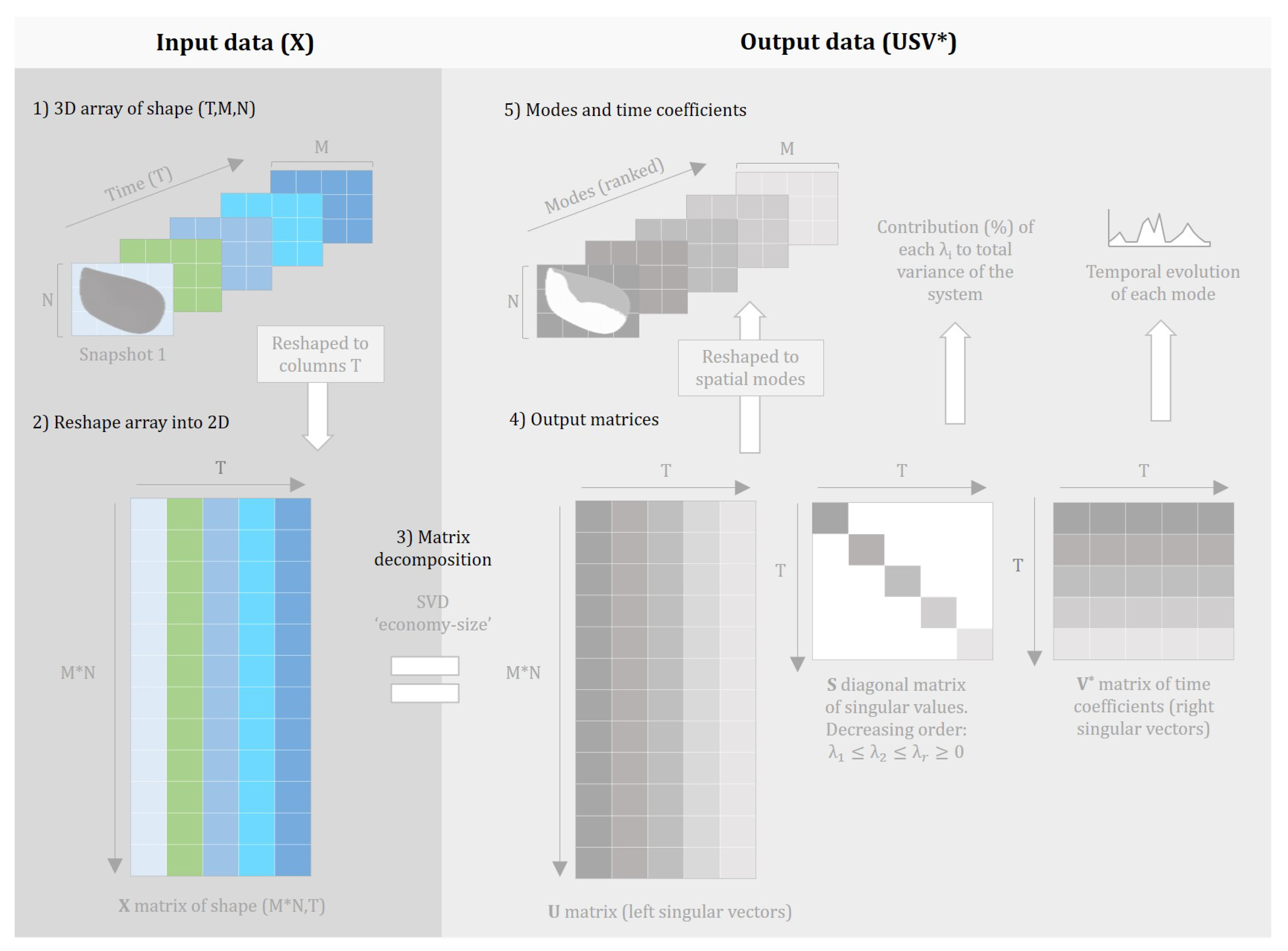
2.2. Proper Orthogonal Decomposition

Proper orthogonal decomposition (POD) is a statistical method that can be used to elucidate the most important features (modes) from a complex system, such as time series or spatial data, by finding a set of orthogonal basis vectors that capture the dominant patterns of variation. Essentially, it is a tool to simplify big datasets by highlighting the main trends, like identifying the biggest waves in a sea of numbers. This technique is a powerful tool for identifying coherent structures in turbulent flows and is commonly used in fluid dynamics to create approximate low-dimensional descriptions of nonlinear, highly complex processes [28,48]. As a ‘proper’ or optimal method, it maximizes the variance that can be captured by the first n spatial modes. The orthonormal property of each mode implies that each time coefficient depends on the spatial mode.
The method we choose to compute the POD is the direct method via a Singular Value Decomposition (SVD), as opposed to the snapshot method [49,50]. In our study, we compute POD by constructing an N × T data matrix X = [ X 1 , X 2 , , X T ] whose columns are formed from mean subtracted vectors formed from individual stacked vectorized data fields of TEM, RH, PM2.5, and PM10 ( x t ) at regular time intervals (t = 1 , 2 , , T ). An ‘economy-size’ SVD (where only the first T columns of X are computed) is performed on X :
X = US V *
where (*) is a conjugate transpose, U is an N × N orthogonal matrix of left singular vectors, arranged as columns; V * is a T × T orthogonal matrix of right singular vectors arranged as rows, and S is a T × T diagonal matrix of singular values in descending order along the diagonal i.e., σ 1 σ 2 σ 3 σ r 0 . The left orthogonal vectors in matrix U correspond to the spatial modes. The right singular vectors V* correspond to the eigenvectors, the time coefficients that describe the temporal evolution of each mode. The eigenvalues or singular values S quantify the contribution or energy captured by each mode. The spatial modes U are ranked by their importance, or variance, as determined by the eigenvalues S , which means the modes are ranked by their contribution to the total variability of the system. The relative importance of each mode can be computed via the following:
Contribution   ( % ) the   i th   singular   value = λ i 2 j = 1 r λ j 2 × 100
where λ i 2 denotes the i t h singular value, r is the rank of the matrix (non-zero singular values taken from the diagonal of S ), and j = 1 r λ j 2 × 100 is the sum of the squares of all non-zero singular values. The result is the contribution of the i t h singular value to the total variance of the matrix. In this study, we have integrated PM2.5, PM10, temperature, and humidity data into the input matrix for the POD analysis. This integration is justified by the inherent interconnections among these environmental parameters, where temperature and humidity influence PM dispersion through processes like convection and hygroscopic growth, potentially affecting mode separation but also enriching the physical interpretability of the modes by capturing coupled effects. POD allows us to extract dominant spatial and temporal patterns while preserving the physical interpretation of the resulting singular values. An illustrated diagram of the POD computation is shown in Figure 2.
From a physical interpretation, the POD can be used to gain a spatial picture of patterns that are repeating or coherent through a time series. The evolution of these modes through time, extracted from the eigenvectors V * , can be particularly important as it allows us to see particular trends and their repeatability which can be quantified through a Fourier power spectrum [31]. In short, POD allows us to look for patterns that are important in space, rank how these elucidated patterns relate to one another, and to what extent these patterns are important and repeatable through time. It is worth mentioning that other techniques such as dynamic mode decomposition (DMD) can also be used to extract structures from complex datasets. Unlike POD, DMD explicitly seeks to capture dynamic behavior within a system [51] and is commonly employed on very detailed spatial resolution.

3. Results and Discussion

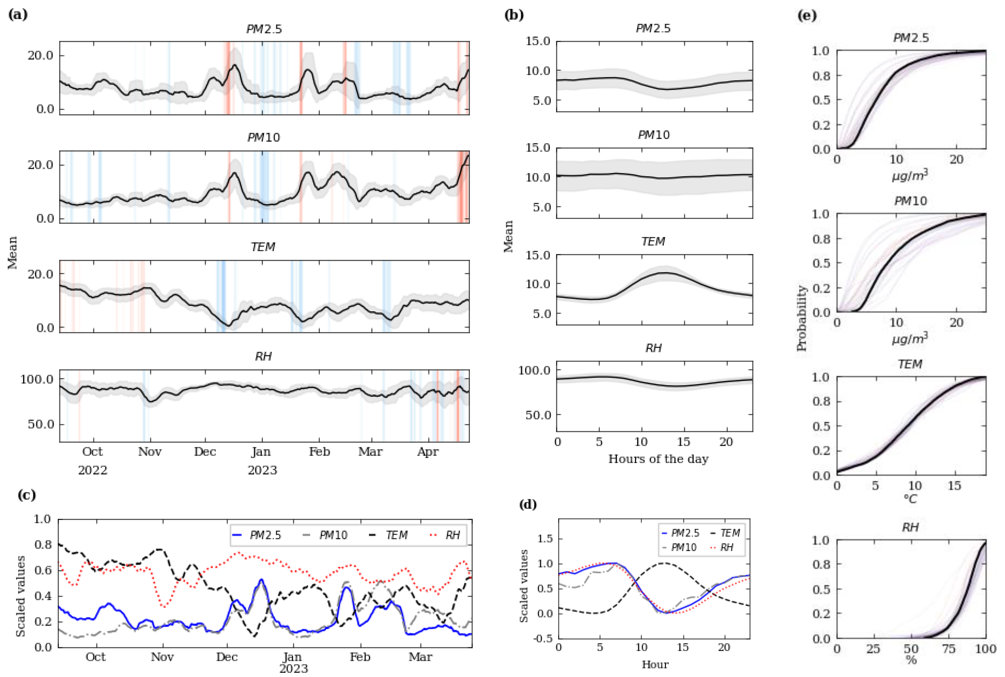
3.1. Data Analysis—Descriptive Statistics

In Figure 3, we present the time series data captured by each individual sensor and average daily patterns of PM2.5 and PM10, TEM, and RH. The time series data in Figure 3a show a cyclic pattern of peaks and drops for both PM10 and PM2.5. During the winter of 2022, particularly in early- to mid-December, late January, and early February, pollution levels increased significantly. These increases match the periods with the lowest TEM values. Similarly, in the period ranging from late December to mid-January, outdoor PM levels dropped significantly in the LCR while TEM increased; these simultaneous changes suggest an association between TEM and PM. One potential link to TEM is the changes in domestic combustion, an activity that increases when temperatures drop. Most emissions from this source come from households burning wood in closed stoves and open fires [52].
As 2023 progressed, PM2.5 reduced while PM10 levels continued around 10 μg/m3 throughout March and April, increasing significantly by the end of April. On the other hand, the diurnal patterns observed in Figure 3b include an increase in PM from 7:00 to 8:00, with a second PM increase around 19:00–20:00 h. These peaks in PM could be linked with increased traffic related to commutes to workplaces and school hours. In contrast, the lowest levels are observed around midday when TEM records are the highest; the reason may be that high temperature promotes the convection of air, leading to the dilution and diffusion of air pollutants [53].
The normalized time series in Figure 3c showed a significant increase in PM2.5 and PM10 in December that matched reductions in TEM, supporting the records shown in Figure 3a. This was followed by a reduction in PM as TEM rose. Similarly, reductions in TEM in late January and February 2023 were linked to increases in PM, particularly PM10. A snapshot into the diurnal patterns of these variables (Figure 3d), shows levels of PM to be the highest in the early morning before dropping significantly from 10:00 to 16:00, a behavior similarly recorded for RH. These variable changes are contrasted with the daily increase in TEM peaking at midday. The variation between the different sites (particularly PM10) highlights the need for a method that can differentiate the impacts of spatial variability across the LCR.
In Figure 3e, we present cumulative distribution functions (CDFs) to gain insight into the probabilistic distributions of the data. The CDF shows that 50% of PM2.5 and PM10 values were below 7.5 μg/m3. For PM2.5, the majority (80%) of values were below 15 μg/m3. Similar records were observed for PM10, however, for this pollutant there were more events of extreme records reaching more than 25 μg/m3. While these values comply with the UK’s Air Quality Standards and Regulations [52], they exceed significantly the most recent Air Quality Guidelines from the WHO [54], which state that PM2.5 and PM10 should not exceed an annual average of 5 μg/m3 and 15 μg/m3, respectively.
Analyzing one-dimensional representations of air quality data can reveal notable disparities in air quality among different regions of the LCR at any given time. However, fully comprehending the implications of these disparities can be challenging. Among these implications, understanding the contribution of specific urban areas to the concentration of air pollutants is of utmost importance. Similarly, aspects of urban development could impact the urban heat island effect, and the presence of a shoreline in a port city like the LCR may exert a significant influence on the local climate [55]. To gain a comprehensive understanding of these disparities, it is necessary to perform a spatial interpretation of the data. By visually correlating disparities across the LCR, we can gain invaluable insights into how specific events within the urban environment can contribute to increased levels of pollutants, changes in RH, and temperature.

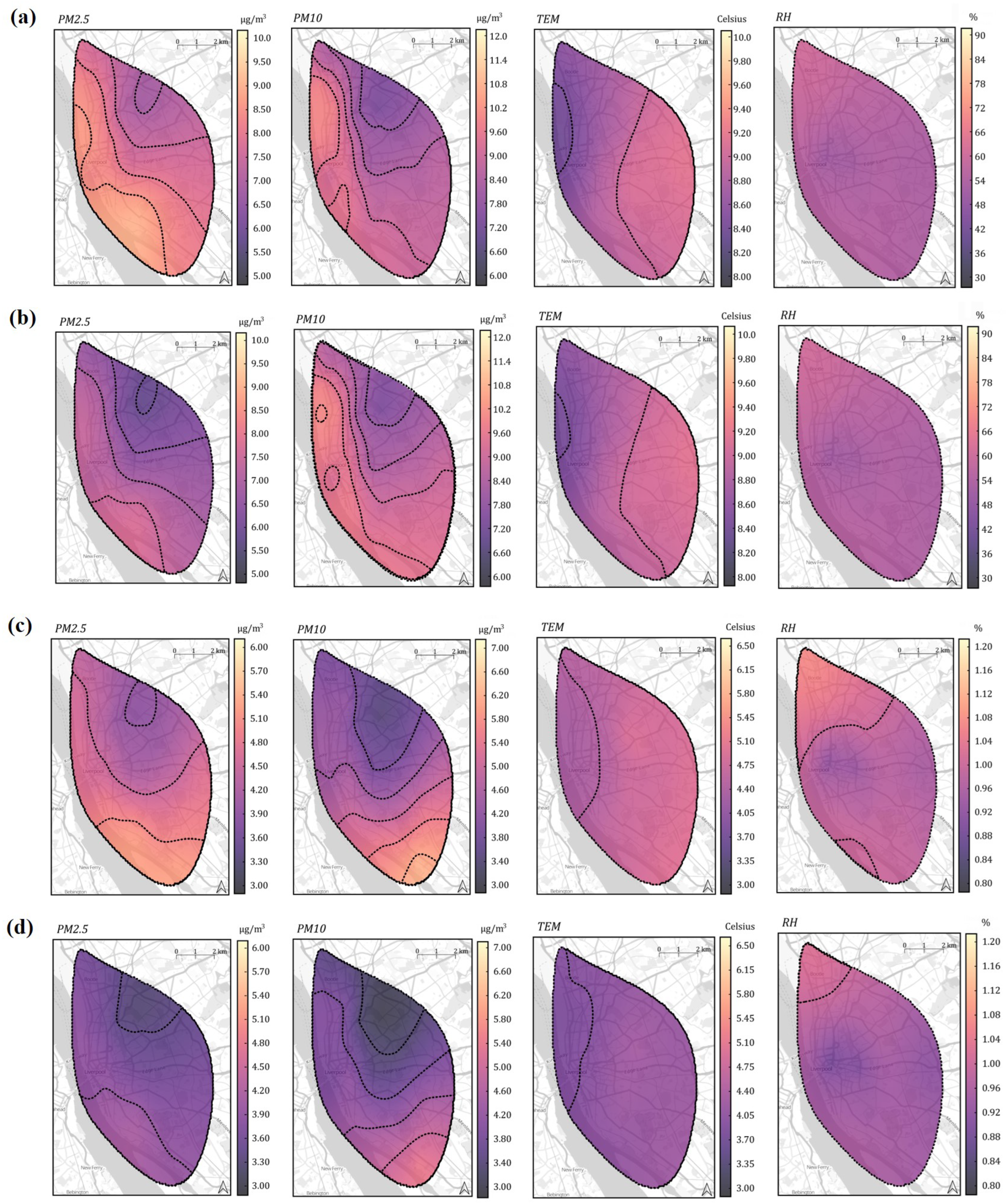
3.2. Data Analysis—Spatial Interpolation

To gain a deeper insight into the spatial distribution of the PM, RH, and TEM we create a set of spatial maps as per Higham et al. [56] but at a local scale. We begin by investigating the first-order statistics of the time series, a set of basic measures of central tendency and dispersion. The mean and standard deviation represented spatially, provide insight into the magnitude of pollutants across the time series. This helps to physically identify areas where there are significant concentrations of pollutants.
The spatial representations in Figure 4a,b reveal the highest levels of PM are seen near the LCR center. In Figure 4a, the 250-day average shows consistently high levels of PM2.5 in most of the LCR, and decreased levels near residential areas in the northeast of the study area. When comparing with its daily pattern (averaged across all hours within each day and all days), the 250-day averaged pollution levels are significantly higher. This suggests that events with high levels of PM are influencing the overall representation of pollution but may not display a daily frequency.
PM10 also shows increased levels along the River Mersey and main traffic roads along the docks, with the highest levels observed in two main hotspots: one located near the center of the LCR, to the south in a residential area, and to the north near a substantial construction site. This is observed in the 250-day average and in the daily patterns, as shown in Figure 4a,b. Furthermore, areas with higher PM10 levels also exhibit lower TEM values, supporting the inverse relationship observed between TEM and PM in Figure 3c,d. It is worth considering that TEM could be influenced locally by the proximity to the river Mersey [57]. This proximity is a distinctive feature of the LCR, and the areas closer to the river also experience higher commercial activities and traffic.
Figure 4c,d show a spatial representation of the standard deviations of pollution and meteorological variables measured by the WSN. From a physical perspective, the standard deviation provides valuable information about the time series by highlighting significant variations between high and low levels. Unlike the mean, the standard deviation uncovers hidden spatial patterns within the data, specifically becoming a useful tool in pinpointing regions with notable fluctuations in pollutant concentrations.
PM2.5 exhibits the highest standard deviation values in most of the study area for the 250-day average, indicating that isolated events with extreme values strongly influence the interpolated average patterns. Conversely, daily patterns of PM2.5 capture low standard deviations, suggesting that the fluctuations in pollution levels throughout the day do not reach extreme extents. Similarly, PM10 displays higher standard deviations in its 250-day spatial pattern, with significant standard deviations observed in its daily pattern, specifically in the southern region of the study area. Additionally, TEM and RH exhibit higher standard deviations in their overall averages, potentially due to seasonal and meteorological events. However, their daily patterns show little change, implying that their fluctuations are less extreme on a daily basis.
Spatial representations based on first and second-order statistics provide valuable insights into the variations in pollutant concentrations across a city. While they are beneficial to understanding spatiotemporal patterns, these representations only offer a snapshot view of the data at a given time. As shown by the single point statistics, the time series of PM and weather variables are clearly subject to change. Consequently, these methods fail to capture changes arising from seasonal variation and cyclic patterns, and the correlations between spatial and temporal events. Moreover, due to their inherent nature, certain statistics may inadvertently mask cyclic sinusoidal-like events. Therefore, in this study, we turn to the POD to decompose the time series of data into spatial modes and temporal modes. By employing the POD, we can effectively capture both spatial and temporal correlations in the data, enabling us to gain deeper insights into the dynamics of air pollutants within the LCR.

3.3. Proper Orthogonal Decomposition
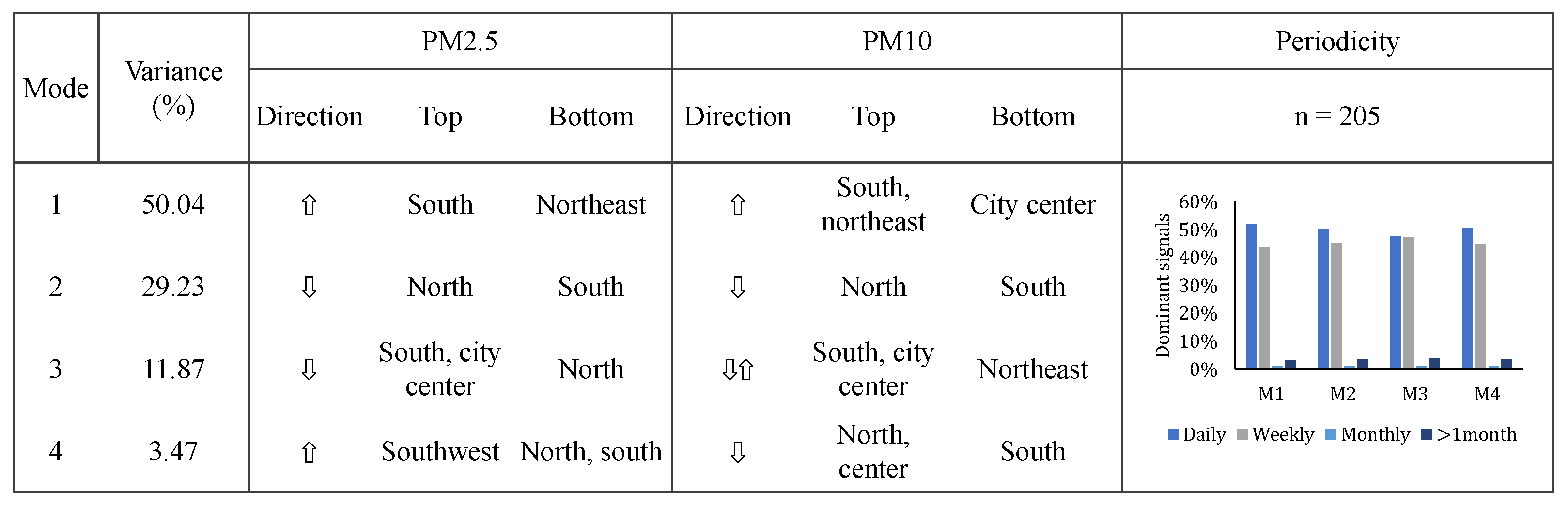
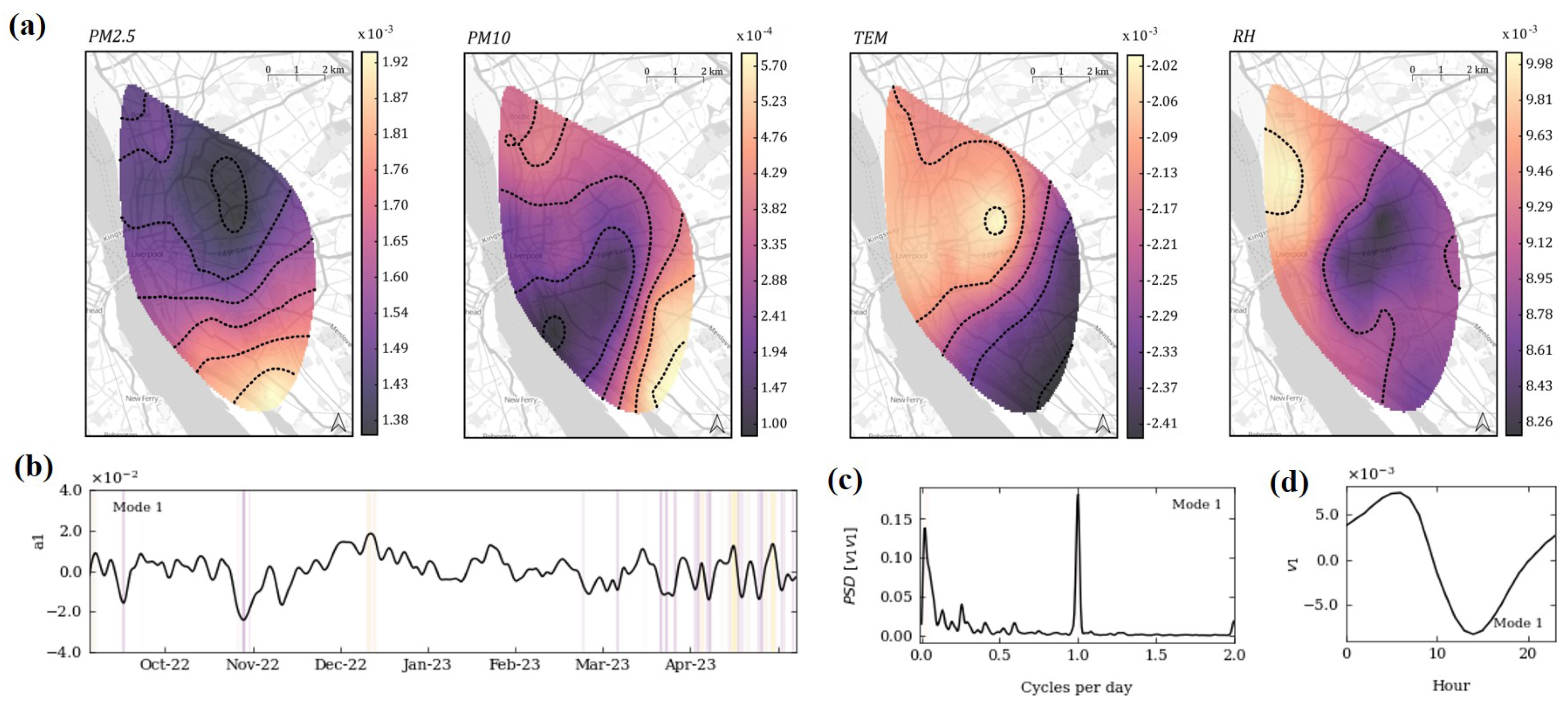
The POD can be used to extract spatially coherent patterns from a time series. By simultaneously inputting RH, TEM, and PM, it is possible to extract spatial correlations in time as well as find coherence or similarities across variables. In fluid mechanics, the POD is commonly used to find relationships between streamwise and spanwise components. Similarly, it can be used to find correlations between meteorological factors and pollution levels.
The first 10 modes account for a contribution of 98.84% to the total variance of the dataset (a detailed depiction of each mode contribution is shown in Appendix B). This contribution was calculated as depicted in Equation (1). Figure 5, Figure 6, Figure 7 and Figure 8 present the first four modes, which together account for 94.61% of variance in the dataset. Unlike conventional POD approaches in other studies [35], there is an absence of a clear quasi-conjugate relationship between the first two modes. This absence suggests minimal or negligible interaction between the top four modes.
Mode 1 ( U 1 ) is the dominant mode, with 50.04% of the variance attributed to its singular value. This suggests that U 1 is a reliable approximation for describing the overall pattern of variables’ changes in the LCR. It is noteworthy that U 1 contributes to nearly twice the variance compared to the second mode. Consequently, it is reasonable to anticipate that U 1 among all spatial distributions will encompass the most significant alterations, while the second mode might capture harmonics or even finer-scale distribution shifts present in the data.
U 1 patterns, depicted in Figure 5a, reveal a positive correlation between PM2.5 and PM10 across all locations. The changes in U 1 vary across the LCR, indicating that the sources driving these alterations can be localized, rather than just a large-scale process influencing the rate of change in PM levels across the entire area. For PM2.5, greater changes happen in the south of the study area (both increases and decreases), transitioning toward fewer changes in the northeast. This aligns well with the standard deviation and mean depicted in Figure 4. PM10 also exhibits greater changes in the south of the study area, while the lowest magnitudes are observed in the center of the LCR, particularly around the docks. However, it should be noted that PM10 changes are an order of magnitude smaller than those of PM2.5.
As expected, TEM and RH changes are coupled. In the northwest area of the study, particularly around the docks, the flux of simultaneous TEM and RH changes is significant. For TEM, the direction of changes is opposite in the southeast (suburban stations). These patterns could be indicative of localized phenomena influencing the rate of TEM changes near the city center, such as the urban heat island effect, the regulating effect of a water body along the docks, and other meteorological parameters. Interestingly, this pattern of changes is not as clear in the standard deviations from Figure 4, highlighting the complexity of TEM and RH distribution in the city that can be elucidated through POD.
The temporal coefficients ( V 1 ) corresponding to U 1 are shown in Figure 5b. A cyclical pattern is observed, with larger peaks in mid-December 2022, and late January 2023, and consecutive peaks and troughs in the spring of 2023. These peaks indicate increases in the flux of PM and a decrease in TEM variation. This is likely attributed to cold spells and anthropogenic events leading to increased levels of PM, as recorded in Figure 3a. To assess the periodicity of U 1 , we apply a Pwelch Fourier power spectral density (PSD) analysis on the temporal coefficients (Figure 5c). The dominant frequencies of 1 day relate to the diurnal pattern of the variables. While the top signal showed a daily periodicity, a secondary peak shows a periodicity of ~1 month on average, followed by signals with higher timescale. This suggests that U 1 is strongly influenced by anthropogenic changes given by daily and weekly activities, as supported by Figure 5d with positive magnitudes in the morning and evening. On the other hand, signals with higher timescales could be indicative of natural fluctuations driven by seasonal changes.
Figure 6 illustrates the second mode ( U 2 ), which accounts for 29.23% of the total variance. In contrast to the first mode, the U 2 patterns for PM10 and PM2.5 are very similar to each other, showing simultaneous reductions across the LCR (Figure 6a). The lowest magnitudes were observed in the south of the city. It should be noted that the variance explained by the eigenvalue is approximately half of the observed for U 1 , thus, the impact of these changes will be less than those of U 1 . On the other hand, TEM and RH changes are not coupled. It seems that the most significant TEM changes occur in the south of the city, whilst the opposite pattern is observed in RH, which also exhibits a similar pattern to PM in U 2 . The areas with higher TEM values tend to decrease in PM more significantly in U 2 , supporting the inverse relationship observed in Figure 3. Some spatial features of RH are similar between its U 1 and U 2 , the magnitudes are notably higher for U 2 .
Figure 6b displays the temporal coefficients of U 2 , which exhibit significant variation over the 250 days, with significant changes in mid-December to late December 2022, late January to mid-February 2023 and late April 2023. When compared to the time coefficients of U 1 , the contribution of U 2 exhibits a few opposite trends, as supported by the daily pattern depicted in Figure 6d. The power spectral density (PSD) plot in Figure 6c indicates that U 2 has dominant frequencies ranging from a week to 2 months, with the strongest signal displaying a periodicity of 43 days. The majority of peak signals showed a 1-month or weekly periodicity, followed by signals with a higher timescale.
The frequencies from Figure 6c correspond to discernible shifts in activities on a weekly or fortnightly basis, with a fortnightly pattern emerging as a harmonic of the weekly pattern with additional variations occurring during weekends. This insight suggests that across the span of a week, substantial changes manifest in the northern part of the city. Conversely, the preceding U 1 highlights alterations in the southern regions concerning PM. Evidently, U 1 describes diagonal patterns, likely driven by TEM, while U 2 sheds light on shifts in weekly or fortnightly cycles.
Figure 7 and Figure 8 depict the two modes U 3 and U 4 , which account for 15.34% of the total variance of the system. Despite their lower contribution, these modes play a crucial role in accurately reconstructing the original variables and revealing overlooked patterns. U 3 shows negative changes throughout the LCR (Figure 7a) with the lowest magnitudes in the northern regions and higher magnitudes in the center and south of the study area. A similar pattern is observed for PM10 with the lowest magnitudes in the northeast.
The variations in the directions of PM10 changes, with simultaneous increases in the south and decreases in the north, may reflect the movement of pollution throughout the city due to transport and emissions sources. In this vein, U 3 exhibits some similarities to the standard deviation in Figure 4, particularly for PM10, with increases in the south. TEM patterns in U 3 differ significantly from U 1 , U 2 , and Figure 4a, displaying simultaneous decreases in U 3 with higher magnitudes in the center of the LCR and along the northern docks. Meanwhile, RH displays correlated negative magnitudes in the north of the study area and positive values in the furthest south.
The temporal coefficients ( V 3 ) exhibit a gradual change in the contribution of this mode, as illustrated in Figure 7b. The PSD analysis (Figure 7c) reveals that the dominant frequency in U 3 is 57 days. The highest peak of dominant signals depicted in Figure 7c exhibits an average periodicity of 34 days with the smallest periodicity of 2 weeks and the highest of 3 months. Additionally, U 3 exhibits a less prominent daily signal compared to the other temporal modes, while its daily pattern shares similarities with U 1 (Figure 7d). The patterns identified in U 3 are likely associated with seasonal mid-term changes (frequencies > 1 month), as well as short-term meteorological changes and anthropogenic influences.
U 4 (Figure 8a) is the last mode analyzed in this study, exhibiting similar PM10 features to those observed in U 2 , albeit to a lesser extent. In contrast, the direction of PM2.5 U 4 is opposite to the observed in U 2 and U 3 . PM2.5 changes exhibit simultaneous increases across the study area and a significant difference in the magnitude of changes south to the center of the LCR. This area covers residential areas and also urban features with a transition to commercial and industrial features. Although the contribution of U 4 to the total variance is limited, with a 3.47%, this mode may point to isolated events or changes over time that resulted in correlated changes in pollutant magnitudes across specific regions. Similar to U 1 , TEM patterns in U 4 display correlated decreases across the LCR, while RH patterns show both correlated increases and decreases. The temporal coefficients of U 4 vary significantly throughout 2023 (Figure 8b), with PSD frequencies revealing a predominant frequency of 21 days. This is followed by other dominant signals at weekly and monthly timescales, and a smaller signal with a daily periodicity, whose daily patterns (Figure 8d) is similar to U 1 and U 3 . The majority of the top signals in U 4 exhibit weekly frequencies (Figure 8c).
We can extract the following findings for each mode (summarized in Appendix B Figure A2):
  • The dominant U 1 shows correlated increases in the whole of the study area. PM2.5 pollution changes more in the south of the LCR, while PM10 increases both in the southern and northern regions, albeit to a lesser extent. The dominant periodicity of U 1 is daily, suggesting cyclic components such as TEM and RH linked to the pollution level changes in U 1 . However, considering that the spatial correlation between the meteorology variables and pollution levels in Figure 4 is not clear-cut, anthropogenic factors could also be driving PM changes. This is supported by the daily patterns of the U 1 time coefficients, in which the positive contributions of the PM mode are observed in the morning and evening. Overall, the increases in pollution levels can be linked to both temperature and changes in traffic, potentially due to transport from residential areas to workplaces.
  • U 2 
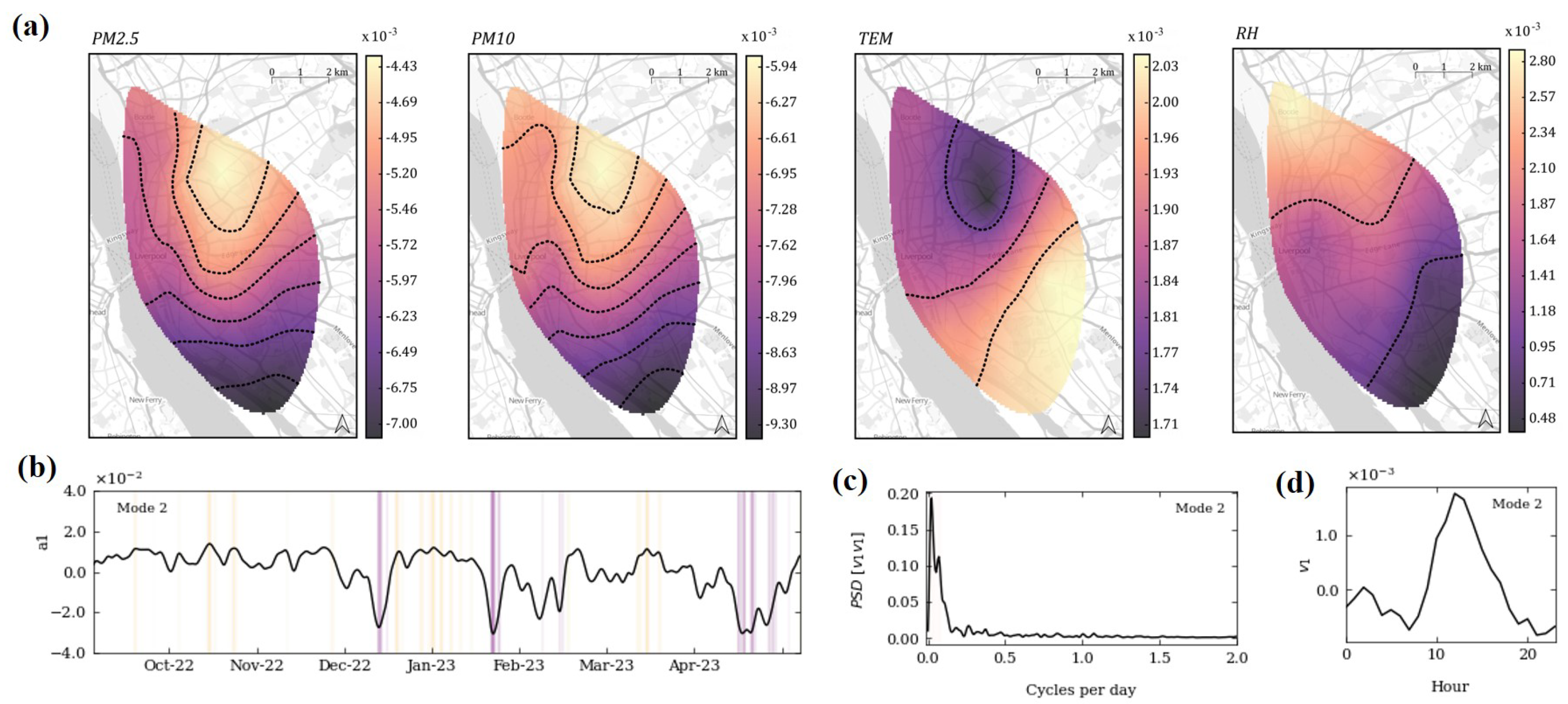
shows positive correlations with simultaneous reductions in PM. The patterns of PM2.5 and PM10 changes in U 2 share similarities between both pollutants suggesting a common source driving their changes. Areas with higher TEM positive changes experience more significant negative changes in PM magnitudes, supporting the inverse relationship observed in Figure 3. The most dominant frequencies showed weekly to 1-month periodicity, corresponding to shifts in activities on a weekly and fortnightly basis.
  • PM2.5 decreases at varying rates across the LCR in U 3 , with higher reductions in the north compared to the south. PM10 tends to increase significantly from the center to the southern regions, with lower increases observed in the northeast. These simultaneous variations could reflect the movement of pollution throughout the LCR. U 3 dominant frequency is 57 days, and it may be associated with seasonal short-term changes (top 10 dominant frequencies ~1 month), as well as cyclic components such as temperature, considering its daily pattern.
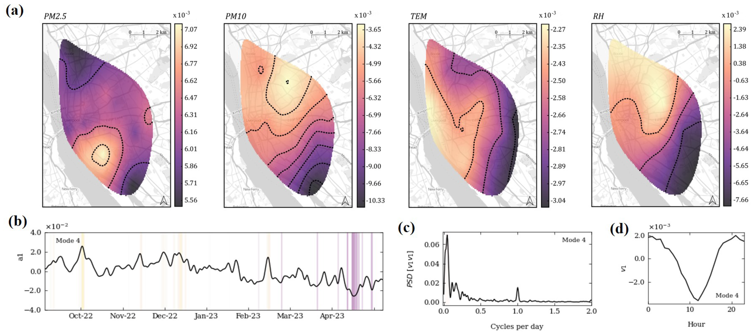
  • In U 4 , PM2.5 increases across the study area with higher increases in the changes across residential and urban areas transitioning into commercial/industrial features. In contrast, PM10 magnitudes decrease in the south of the LCR. While the U 4 contribution is limited, this mode may indicate isolated events or temporal changes resulting in correlated pollutant changes in specific regions. Temporal coefficients ( V 4 ) vary significantly throughout 2023, with a dominant frequency of 21 days. Its daily pattern is similar to U 1 and U 3 , suggesting that these modes might share common sources or behavior.
To strengthen the causal interpretation of these modes, future work could correlate them with external datasets. For instance, Mode 1’s daily periodicity aligns with peak commuting hours, suggesting a link to traffic counts from Liverpool City Council’s traffic monitoring systems. Mode 3’s pollution transport patterns could be validated against wind direction and speed data from local meteorological stations, enhancing the physical basis of these findings.

3.4. Implications for Urban Air Pollution Management

The need for sustainable development in the context of urbanization has led to concepts such as Smart Cities, which focus on innovative technologies including sensors, and data-driven insights to improve the quality of life [58,59]. As a result, the number of WSN deployments sensing changes in environmental features such as air pollution has significantly increased [60,61]. This study demonstrates the benefits of WSN for capturing air quality data at higher resolutions to identify temporal trends and spatial patterns.
Granular spatial data are crucial for developing targeted policies to address high pollution events [62] and reduce the intensity of pollution hotspots. Moreover, the availability of high-resolution data allows the implementation of numerical methods such as POD. The results from the application of POD in our study highlight the significant temporal variability in the patterns of PM.
The temporal variability is particularly important for the detection of PM hotspots [63]. Traditionally, areas that exhibit high pollutant averages are categorized as pollution hotspots and managed accordingly. However, the identification of hotspots of significant changes in pollution through POD highlights their dynamic features. This implies that the management of areas with pollution hotspots is not straightforward and should consider mobile sources of air pollution and the frequency at which citizens could be exposed.
In our study, the dominant daily mode draws attention to the impact of commuting in residential areas, emphasizing the urgency of incorporating effective traffic management strategies. Mode 1’s diurnal peaks suggest targeted traffic calming measures, such as time-specific low-emission zones in southern residential areas during morning and evening commutes, while Mode 3’s transport patterns indicate a need for wind-informed routing of heavy vehicles near the city center to mitigate pollution spread. The variability in magnitudes for each mode suggests the effect of localized phenomena on the distribution of PM, supporting the need for local measures that mitigate disparities among different neighborhoods, such as green areas. Furthermore, the detection of frequencies for each observed pollution pattern can help regulate citizens’ exposure and reduce the impacts of air pollution on vulnerable groups.
Decision-makers could use these findings to implement real-time air quality alerts during peak Mode 1 h, optimize sensor placement in southern hotspots identified by Mode 1, and adjust industrial schedules near the center based on Mode 3’s transport patterns, enhancing urban air quality management with data-driven precision.
In practice, POD offers an efficient method for analyzing near real-time air pollution data by capturing complex patterns and correlations between pollution and meteorological variables. However, the uneven sensor coverage, with sparser nodes in the northern LCR, may introduce interpolation errors, potentially underrepresenting pollution dynamics in those areas. This limitation of spatial resolution could be addressed in future deployments by increasing sensor density in underrepresented regions. The application of POD can be integrated into decision support systems for managing extreme pollution events, implementing air quality targets, and understanding pollution hotspots.

4. Conclusions

In this study, we discuss the application of proper orthogonal decomposition (POD) for analyzing air pollution and meteorology variables. The application of this technique is driven by the deployment of wireless sensor networks (WSNs) that capture high-resolution spatiotemporal data. We compare the results of traditional time series analysis, spatial representations, and POD from a dataset produced by a WSN in the Liverpool City Region (LCR) in the United Kingdom.
The results of the temporal analysis show an increase in pollution levels in December 2022, January 2023, and February 2023. These increases appear to be inversely correlated with temperature, with pollution levels reaching their lowest point at midday. Half of the PM values were lower than 7.5 μg/m3, and extreme events were recorded, especially for PM10. While these values comply with the UK Air Quality Standards Regulations of 2010, they exceed the air quality guidelines set by the WHO in 2021. To complement the time series analysis, we performed a spatial interpolation. The spatial distribution revealed that the highest PM2.5 values were recorded in the center of the LCR. While PM10 hotspots were observed near the center of the LCR, these also covered residential areas. The 250-day average spatial representation shows values higher than the daily representations, suggesting that extreme pollution events might be influencing the overall computations. This was supported by the standard deviation, with higher values for PM2.5. For PM10 the standard deviation was highest in the south of the study area, including residential spaces. These representations gave us insight into the pollution levels on-site, however, they failed to capture the variability arising from cyclic patterns and seasonal variations.
To perform a higher-resolution analysis of these data, we applied the POD and decomposed the time series into modes. Four dominant modes were discussed as they accounted for 94.61% of the total variance of the system. In the dominant U 1 , PM2.5 correlates positively throughout the study area, with higher magnitudes in the south. This mode shows a daily periodicity and it is influenced by cyclic components and likely anthropogenic factors. Morning hours have the greatest contributions, potentially reflecting increased traffic from residential areas to workplaces, a hypothesis that could be confirmed with traffic flow data from Liverpool authorities. In U 2 , simultaneous reductions in PM levels are observed, and higher temperature areas record greater PM reductions. This mode is similar between PM2.5 and PM10, suggesting a common source. U 2 patterns show a weekly and fortnightly periodicity. In U 3 , PM2.5 decreases at varying rates across the LCR, while PM10 increases significantly from the center to the south. These simultaneous increases and decreases reflect the dynamics of pollution throughout the LCR. This pollution transport hypothesis could be validated with meteorological data, such as wind direction and speed from LCR stations. On the other hand, U 4 shows significant differences in the magnitudes of PM2.5 changes near the city center, which might point to isolated events of air pollution, considering the variability of its time coefficients.
Overall, the POD allowed us to see patterns that were not easily discernible from the traditional spatiotemporal representations. The dominant patterns were not indicative of the averaged spatial representation, but a detection of correlations that could be driven by common factors. This is important in order to target interventions for improving air quality. Additionally, the time coefficients given by POD allowed us to see an evolution of each of the detected modes, and pinpoint specific events in time where each of the modes was more active. This, coupled with the Fourier power spectra, allowed us to identify the cyclicity of each pattern and its association with anthropogenic activities. This result offers advantages versus the time series data as it considers both the spatial movements of pollution and the changes through time. Therefore, the POD helps identify where pollution levels may change more significantly at any given time and targets initiatives to limit citizens’ exposure. This level of detail was not achieved from time series or spatial distributions alone. It is worth noting that, while the patterns reflect urban and anthropogenic features of the study area, the modes observed in this study reflect areas of correlation and are not an indication of pollution concentrations, as they are usually measured and analyzed through other methods. Therefore, a careful environmental interpretation of each mode should be performed.

Author Contributions

C.A.R. undertook the data analysis and writing of the text, J.E.H. conceived the idea and supervised the work. All authors have read and agreed to the published version of the manuscript.

Funding

Funding comes from CONACYT Mexico in funding the studies of C.A.R.

Data Availability Statement

Data will be made available upon request.

Conflicts of Interest

The authors declare that they have no known competing financial interests or personal relationships that could have appeared to influence the work reported in this paper.

Appendix A. POD Pseudocode

Algorithm A1: Proper orthogonal decomposition (POD)
Urbansci 09 00166 i001
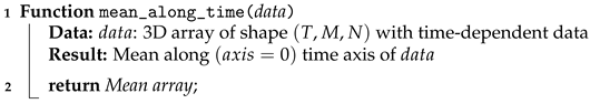
Algorithm A2: Function: mean_along_time
Urbansci 09 00166 i002
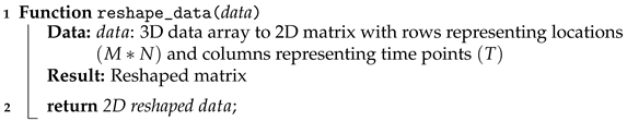
Algorithm A3: Function: reshape_data
Urbansci 09 00166 i003
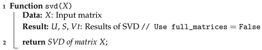
Algorithm A4: Function: svd
Urbansci 09 00166 i004
Algorithm A5: Function: create_diagonal_matrix
Urbansci 09 00166 i005

Appendix B. Modes Details

Figure A1. Contribution of the first 10 modes to the total variance in the dataset. Highlighted in the box are the details of the contributions of modes 4–6.
Urbansci 09 00166 g0a1
Figure A2. Summary of findings for each mode, where periodicity has a sample of 10% of the total signals (n = 205).
Urbansci 09 00166 g0a2

References

  1. WHO. Ambient (Outdoor) Air Pollution; WHO: Geneva, Switzerland, 2023. [Google Scholar]
  2. Bălă, G.P.; Râjnoveanu, R.M.; Tudorache, E.; Motișan, R.; Oancea, C. Air pollution exposure—The (in)visible risk factor for respiratory diseases. Environ. Sci. Pollut. Res. 2021, 28, 19615–19628. [Google Scholar] [CrossRef]
  3. Chen, R.; Jiang, Y.; Hu, J.; Chen, H.; Li, H.; Meng, X.; Ji, J.S.; Gao, Y.; Wang, W.; Liu, C.; et al. Hourly Air Pollutants and Acute Coronary Syndrome Onset in 1.29 Million Patients. Circulation 2022, 145, 1749–1760. [Google Scholar] [CrossRef]
  4. Delgado-Saborit, J.M.; Guercio, V.; Gowers, A.M.; Shaddick, G.; Fox, N.C.; Love, S. A critical review of the epidemiological evidence of effects of air pollution on dementia, cognitive function and cognitive decline in adult population. Sci. Total Environ. 2021, 757, 143734. [Google Scholar] [CrossRef]
  5. Wolf, K.; Hoffmann, B.; Andersen, Z.J.; Atkinson, R.W.; Bauwelinck, M.; Bellander, T.; Brandt, J.; Brunekreef, B.; Cesaroni, G.; Chen, J.; et al. Long-term exposure to low-level ambient air pollution and incidence of stroke and coronary heart disease: A pooled analysis of six European cohorts within the ELAPSE project. Lancet Planet. Health 2021, 5, e620–e632. [Google Scholar] [CrossRef]
  6. Zhu, F.; Ding, R.; Lei, R.; Cheng, H.; Liu, J.; Shen, C.; Zhang, C.; Xu, Y.; Xiao, C.; Li, X.; et al. The short-term effects of air pollution on respiratory diseases and lung cancer mortality in Hefei: A time-series analysis. Respir. Med. 2019, 146, 57–65. [Google Scholar] [CrossRef]
  7. Defra. Air Quality Statistics; Defra: London, UK, 2023.
  8. Alemayehu, Y.A.; Asfaw, S.L.; Terfie, T.A. Exposure to urban particulate matter and its association with human health risks. Environ. Sci. Pollut. Res. 2020, 27, 27491–27506. [Google Scholar] [CrossRef]
  9. Arias-Pérez, R.D.; Taborda, N.A.; Gómez, D.M.; Narvaez, J.F.; Porras, J.; Hernandez, J.C. Inflammatory effects of particulate matter air pollution. Environ. Sci. Pollut. Res. 2020, 27, 42390–42404. [Google Scholar] [CrossRef]
  10. Liu, C.; Chan, K.H.; Lv, J.; Lam, H.; Newell, K.; Meng, X.; Liu, Y.; Chen, R.; Kartsonaki, C.; Wright, N.; et al. Long-Term Exposure to Ambient Fine Particulate Matter and Incidence of Major Cardiovascular Diseases: A Prospective Study of 0.5 Million Adults in China. Environ. Sci. Technol. 2022, 56, 13200–13211. [Google Scholar] [CrossRef]
  11. Psistaki, K.; Achilleos, S.; Middleton, N.; Paschalidou, A.K. Exploring the impact of particulate matter on mortality in coastal Mediterranean environments. Sci. Total Environ. 2023, 865, 161147. [Google Scholar] [CrossRef]
  12. Guo, Q.; Zhang, K.; Wang, B.; Cao, S.; Xue, T.; Zhang, Q.; Tian, H.; Fu, P.; Zhang, J.J.; Duan, X. Chemical constituents of ambient fine particulate matter and obesity among school-aged children. Sci. Total Environ. 2022, 849, 157742. [Google Scholar] [CrossRef]
  13. Lin, L.Z.; Zhan, X.L.; Jin, C.Y.; Liang, J.H.; Jing, J.; Dong, G.H. The epidemiological evidence linking exposure to ambient particulate matter with neurodevelopmental disorders: A systematic review and meta-analysis. Environ. Res. 2022, 209, 112876. [Google Scholar] [CrossRef]
  14. Park, S.J.; Lee, J.; Lee, S.; Lim, S.; Noh, J.; Cho, S.Y.; Ha, J.; Kim, H.; Kim, C.; Park, S.; et al. Exposure of ultrafine particulate matter causes glutathione redox imbalance in the hippocampus: A neurometabolic susceptibility to Alzheimer’s pathology. Sci. Total Environ. 2020, 718, 137267. [Google Scholar] [CrossRef]
  15. IQAir. 2024 World Air Quality Report; IQAir Reports; IQAir: Goldach, Switzerland, 2024. [Google Scholar]
  16. Health Effects Institute; UNICEF. State of Global Air 2024: A Comprehensive Analysis of Air Quality and Health Impacts Worldwide; Special Report; UNICEF: New York, NY, USA, 2024. [Google Scholar]
  17. Boogaard, H.; Pant, P.; Künzli, N. Science to Foster the WHO Air Quality Guideline Values. Int. J. Public Health 2025, 69, 1608249. [Google Scholar] [CrossRef]
  18. Hu, K.; Sivaraman, V.; Luxan, B.G.; Rahman, A. Design and Evaluation of a Metropolitan Air Pollution Sensing System. IEEE Sens. J. 2016, 16, 1448–1459. [Google Scholar] [CrossRef]
  19. Patel, H.; Talbot, N.; Dirks, K.; Salmond, J. The impact of low emission zones on personal exposure to ultrafine particles in the commuter environment. Sci. Total Environ. 2023, 874, 162540. [Google Scholar] [CrossRef]
  20. Liang, L.; Daniels, J.; Bailey, C.; Hu, L.; Phillips, R.; South, J. Integrating low-cost sensor monitoring, satellite mapping, and geospatial artificial intelligence for intra-urban air pollution predictions. Environ. Pollut. 2023, 331, 121832. [Google Scholar] [CrossRef]
  21. Gameli Hodoli, C.; Coulon, F.; Mead, M.I. Applicability of factory calibrated optical particle counters for high-density air quality monitoring networks in Ghana. Heliyon 2020, 6, e04206. [Google Scholar] [CrossRef]
  22. Magi, B.I.; Cupini, C.; Francis, J.; Green, M.; Hauser, C. Evaluation of PM2.5 measured in an urban setting using a low-cost optical particle counter and a Federal Equivalent Method Beta Attenuation Monitor. Aerosol Sci. Technol. 2020, 54, 147–159. [Google Scholar] [CrossRef]
  23. Hassani, A.; Castell, N.; Watne, A.K.; Schneider, P. Citizen-operated mobile low-cost sensors for urban PM2.5 monitoring: Field calibration, uncertainty estimation, and application. Sustain. Cities Soc. 2023, 95, 104607. [Google Scholar] [CrossRef]
  24. Lertsinsrubtavee, A.; Kanabkaew, T.; Raksakietisak, S. Detection of forest fires and pollutant plume dispersion using IoT air quality sensors. Environ. Pollut. 2023, 338, 122701. [Google Scholar] [CrossRef]
  25. Kingsy Grace, R.; Manju, S. A Comprehensive Review of Wireless Sensor Networks Based Air Pollution Monitoring Systems. Wirel. Pers. Commun. 2019, 108, 2499–2515. [Google Scholar] [CrossRef]
  26. Wei, P.; Brimblecombe, P.; Yang, F.; Anand, A.; Xing, Y.; Sun, L.; Sun, Y.; Chu, M.; Ning, Z. Determination of local traffic emission and non-local background source contribution to on-road air pollution using fixed-route mobile air sensor network. Environ. Pollut. 2021, 290, 118055. [Google Scholar] [CrossRef]
  27. Adrian, R.J. Twenty years of particle image velocimetry. Exp. Fluids 2005, 39, 159–169. [Google Scholar] [CrossRef]
  28. Lumley, J.L. The Structure of Inhomogeneous Turbulent Flows. In Atmospheric Turbulence and Radio Wave Propagation; Nauka: Moscow, USSR, 1967; pp. 166–177. [Google Scholar]
  29. Holmes, P.; Lumley, J.L.; Berkooz, G. Proper orthogonal decomposition. In Turbulence, Coherent Structures, Dynamical Systems and Symmetry; Berkooz, G., Lumley, J.L., Holmes, P., Eds.; Cambridge Monographs on Mechanics, Cambridge University Press: Cambridge, UK, 1996; pp. 86–128. [Google Scholar] [CrossRef]
  30. Higham, J.; Brevis, W.; Keylock, C.; Safarzadeh, A. Using modal decompositions to explain the sudden expansion of the mixing layer in the wake of a groyne in a shallow flow. Adv. Water Resour. 2017, 107, 451–459. [Google Scholar] [CrossRef]
  31. Higham, J.E.; Brevis, W.; Keylock, C.J. Implications of the selection of a particular modal decomposition technique for the analysis of shallow flows. J. Hydraul. Res. 2018, 56, 796–805. [Google Scholar] [CrossRef]
  32. Higham, J.E.; Shahnam, M.; Vaidheeswaran, A. Using a proper orthogonal decomposition to elucidate features in granular flows. Granul. Matter 2020, 22, 86. [Google Scholar] [CrossRef]
  33. Higham, J.; Vaidheeswaran, A. Modification of modal characteristics in the wakes of blockages of square cylinders with multi-scale porosity. Phys. Fluids 2022, 34, 025114. [Google Scholar] [CrossRef]
  34. Ashmore, D.W.; Mair, D.W.F.; Higham, J.E.; Brough, S.; Lea, J.M.; Nias, I.J. Proper orthogonal decomposition of ice velocity identifies drivers of flow variability at Sermeq Kujalleq (Jakobshavn Isbræ). Cryosphere 2022, 16, 219–236. [Google Scholar] [CrossRef]
  35. Zhang, B.; Ooka, R.; Kikumoto, H. Spectral Proper Orthogonal Decomposition Analysis of Turbulent Flow in a Two-Dimensional Street Canyon and Its Role in Pollutant Removal. Bound.-Layer Meteorol. 2022, 183, 97–123. [Google Scholar] [CrossRef]
  36. Ashrafi, K. Determining of spatial distribution patterns and temporal trends of an air pollutant using proper orthogonal decomposition basis functions. Atmos. Environ. 2012, 47, 468–476. [Google Scholar] [CrossRef]
  37. Liu, Y.; Liu, C.H.; Brasseur, G.P.; Chao, C.Y.H. Proper orthogonal decomposition of large-eddy simulation data over real urban morphology. Sustain. Cities Soc. 2023, 89, 104324. [Google Scholar] [CrossRef]
  38. Jafarzadeh, S.; Jess, D.B.; Stangalini, M.; Grant, S.D.; Higham, J.E.; Pessah, M.E.; Keys, P.H.; Belov, S.; Calchetti, D.; Duckenfield, T.J.; et al. Wave analysis tools. Nat. Rev. Methods Prim. 2025, 5, 21. [Google Scholar] [CrossRef]
  39. Albidah, A.; Fedun, V.; Aldhafeeri, A.; Ballai, I.; Jess, D.; Brevis, W.; Higham, J.; Stangalini, M.; Silva, S.; MacBride, C.; et al. The temporal and spatial evolution of magnetohydrodynamic wave modes in sunspots. Astrophys. J. 2023, 954, 30. [Google Scholar] [CrossRef]
  40. ONS. How the Population Changed in Liverpool, Census 2021; ONS: London, UK, 2021.
  41. Kottek, M.; Grieser, J.; Beck, C.; Rudolf, B.; Rubel, F. World Map of the Koppen-Geiger climate classification updated. Meteorol. Z. 2006, 15, 259–263. [Google Scholar] [CrossRef]
  42. ICL. Liverpool City Region Combined Authority Health And Economic Impact Assessment Study; ICL: Tokyo, Japan, 2020. [Google Scholar]
  43. Authority, L.C. Improving Our Air Quality 2020. Available online: https://www.liverpoolcityregion-ca.gov.uk/improving-our-air-quality (accessed on 14 April 2025).
  44. Mekki, K.; Bajic, E.; Chaxel, F.; Meyer, F. A comparative study of LPWAN technologies for large-scale IoT deployment. ICT Express 2019, 5, 1–7. [Google Scholar] [CrossRef]
  45. Muller, C.L.; Chapman, L.; Grimmond, C.S.B.; Young, D.T.; Cai, X. Sensors and the city: A review of urban meteorological networks: SENSORS AND THE CITY. Int. J. Climatol. 2013, 33, 1585–1600. [Google Scholar] [CrossRef]
  46. Cole, B.; De la Barreda, B.; Hamer, A.; Codd, T.; Payne, M.; Chan, L.; Smith, G.; Balzter, H. Corine Land Cover 2018 for the UK, Isle of Man, Jersey and Guernsey; Environmental Information Data Centre: Lancaster, UK, 2021. [Google Scholar]
  47. Higham, J.E.; Brevis, W. When, what and how image transformation techniques should be used to reduce error in Particle Image Velocimetry data? Flow Meas. Instrum. 2019, 66, 79–85. [Google Scholar] [CrossRef]
  48. Hussain, A.K.M.F. Coherent structures—Reality and myth. Phys. Fluids 1983, 26, 2816–2850. [Google Scholar] [CrossRef]
  49. Aubry, N. On the hidden beauty of the proper orthogonal decomposition. Theor. Comput. Fluid Dyn. 1991, 2, 339–352. [Google Scholar] [CrossRef]
  50. Sirovich, L.; Rodriguez, J.D. Coherent structures and chaos: A model problem. Phys. Lett. A 1987, 120, 211–214. [Google Scholar] [CrossRef]
  51. Schmid, P.J. Dynamic mode decomposition of numerical and experimental data. J. Fluid Mech. 2010, 656, 5–28. [Google Scholar] [CrossRef]
  52. Defra. Particulate matter (PM10/PM2.5); Defra: London, UK, 2023.
  53. Luo, J.; Du, P.; Samat, A.; Xia, J.; Che, M.; Xue, Z. Spatiotemporal Pattern of PM2.5 Concentrations in Mainland China and Analysis of Its Influencing Factors using Geographically Weighted Regression. Sci. Rep. 2017, 7, 40607. [Google Scholar] [CrossRef]
  54. WHO. WHO Global Air Quality Guidelines: Particulate Matter (PM2.5 and PM10), Ozone, Nitrogen Dioxide, Sulfur Dioxide and Carbon Monoxide; WHO: Geneva, Switzerland, 2021. [Google Scholar]
  55. WMO. WMO Air Quality and Climate Bulletin No. 4—September 2024. In World Meteorological Organization Bulletin; Released for Clean Air for Blue Skies Day; WMO: Geneva, Switzerland, 2024. [Google Scholar]
  56. Higham, J.E.; Ram’ırez, C.A.; Green, M.A.; Morse, A.P. UK COVID-19 lockdown: 100 days of air pollution reduction? Air Qual. Atmos. Health 2021, 14, 325–332. [Google Scholar] [CrossRef]
  57. Hathway, E.A.; Sharples, S. The interaction of rivers and urban form in mitigating the Urban Heat Island effect: A UK case study. Build. Environ. 2012, 58, 14–22. [Google Scholar] [CrossRef]
  58. Peralta Abadía, J.J.; Walther, C.; Osman, A.; Smarsly, K. A systematic survey of Internet of Things frameworks for smart city applications. Sustain. Cities Soc. 2022, 83, 103949. [Google Scholar] [CrossRef]
  59. Zhang, S.; Niu, T.; Wu, Y.; Zhang, K.M.; Wallington, T.J.; Xie, Q.; Wu, X.; Xu, H. Fine-grained vehicle emission management using intelligent transportation system data. Environ. Pollut. 2018, 241, 1027–1037. [Google Scholar] [CrossRef]
  60. McKercher, G.R.; Salmond, J.A.; Vanos, J.K. Characteristics and applications of small, portable gaseous air pollution monitors. Environ. Pollut. 2017, 223, 102–110. [Google Scholar] [CrossRef]
  61. Cao, R.; Li, B.; Wang, Z.; Peng, Z.R.; Tao, S.; Lou, S. Using a distributed air sensor network to investigate the spatiotemporal patterns of PM2.5 concentrations. Environ. Pollut. 2020, 264, 114549. [Google Scholar] [CrossRef]
  62. Gameli Hodoli, C.; Coulon, F.; Mead, M.I. Source identification with high-temporal resolution data from low-cost sensors using bivariate polar plots in urban areas of Ghana. Environ. Pollut. 2023, 317, 120448. [Google Scholar] [CrossRef]
  63. Considine, E.M.; Reid, C.E.; Ogletree, M.R.; Dye, T. Improving accuracy of air pollution exposure measurements: Statistical correction of a municipal low-cost airborne particulate matter sensor network. Environ. Pollut. 2021, 268, 115833. [Google Scholar] [CrossRef]
Figure 1. (a) Spatial areal extent of the 34 sensors deployed in the Liverpool City Region (UK). (b) Land use for the area of study based on OSM information mapped to CORINE classes [46]. Approximation to center of LCR areas highlighted with a dotted line and significant construction site indicated with the icon.
Urbansci 09 00166 g001
Figure 2. Illustrated diagram of POD computation using the SVD algorithm (‘economy size’). Pseudocode of the POD algorithm can be found in Appendix A.
Urbansci 09 00166 g002
Figure 3. Time series of measured data in Liverpool. (a) Time series of all sites, with the black line indicating the average trend and the gray area indicating the standard deviation. Top and bottom values are respectively highlighted with blue and red vertical lines. (b) Diurnal variations of all variables with the gray area indicating standard deviation. (c) Normalized values for the time series spanning 250 days and (d) normalized daily values. (e) The cumulative distribution function of all variable readings recorded over 250 days in Liverpool.
Urbansci 09 00166 g003
Figure 4. Spatial representation of data measured by the low-cost WSN in Liverpool: (a) 250-day records average, (b) daily patterns, (c) 250-day records standard deviations, and (d) daily standard deviation.
Urbansci 09 00166 g004
Figure 5. (a) First POD spatial mode of all variables of the study. The POD temporal coefficients for mode 1 are shown in panel (b), where vertical lines highlight the days with the highest (yellow) and lowest (purple) values. (c) Power spectral density (PSD) and (d) daily pattern of the time coefficients shown in (b).
Urbansci 09 00166 g005
Figure 6. (a) Second POD mode of all variables of the study. The POD temporal coefficients for mode 2 are shown in panel (b), where vertical lines highlight the days with the highest (yellow) and lowest (purple) values. (c) Power spectral density (PSD) and (d) daily pattern of the time coefficients shown in (b).
Urbansci 09 00166 g006
Figure 7. (a) Third POD mode of all variables of the study. The POD temporal coefficients for mode 3 are shown in panel (b), where vertical lines highlight the days with the highest (yellow) and lowest (purple) values. (c) Power spectral density (PSD) and (d) daily pattern of the time coefficients shown in (b).
Urbansci 09 00166 g007
Figure 8. (a) Fourth POD mode of all variables of study. The POD temporal coefficients for mode 4 are shown in panel (b), where vertical lines highlight the days with the highest (yellow) and lowest (purple) values. (c) Power spectral density (PSD) and (d) daily pattern of the time coefficients shown in (b).
Urbansci 09 00166 g008
Disclaimer/Publisher’s Note: The statements, opinions and data contained in all publications are solely those of the individual author(s) and contributor(s) and not of MDPI and/or the editor(s). MDPI and/or the editor(s) disclaim responsibility for any injury to people or property resulting from any ideas, methods, instructions or products referred to in the content.

