Spatiotemporal Impact of Urbanization on Urban Heat Island Using Landsat Imagery in Oran, Algeria: 1984–2024

Abstract

Urbanization promotes urban infrastructure development and increases artificial impervious surfaces, leading to rising temperatures and urban climate alterations, contributing to the appearance and intensification of the Urban Heat Island (UHI). In this study, a 40-year time series of Landsat images of the city of Oran was used to generate two biophysical indices. The Normalized Difference Built-up Index (NDBI) distinguished built-up areas from non-built-up areas, while a semi-automatic classification produced Land Use/Land Cover (LULC) maps, for a precise analysis of urban sprawl. The results revealed a significant expansion of urban areas, with an increase of 65.28 km² between 1984 and 2024. The Normalized Difference Vegetation Index (NDVI) was used to estimate Land Surface Temperature (LST) by applying the “Mono Window” algorithm for Thematic Mapper (TM) images and the “Split Window” algorithm for Enhanced Thematic Mapper (ETM+) and Operational Land Imager–Thermal Infrared Sensor (OLI–TIRS) images. The surface temperature difference between urban and rural areas increased from 0.36 °C in 1984 to 4.5 °C in 2024, highlighting the intensification of the Surface UHI (SUHI) effect. LST maps also helped to identify the areas most vulnerable to UHI, as well as those where this effect is persistent, corresponding to the Permanent UHI (PUHI).

1. Introduction

Urban population growth has been steadily rising for years, with urban population now encompassing more than half of the global population. According to the United Nations Department of Economic and Social Affairs, it is projected to reach $75\%$ by 2050 [1]. The global urbanization rate is anticipated to increase by $70\%$ relative to the current global population [2], driven by the emergence of new urban areas and the continuous migration of populations from rural to urban and suburban regions. This urbanization process results in profound changes in surface and atmospheric properties, leading to a shift in climatic equilibrium. These changes create a distinctive phenomenon known as urban climate, whose the main feature is the UHI effect [3].

A UHI is characterized by significantly higher temperatures in urban areas compared to their rural surrounding (Figure 1a); an illustration of the UHI is presented in Figure 1b. This phenomenon is primarily attributed to the high thermal capacity of construction materials, reduced latent heat flux caused by increased surface runoff, elevated anthropogenic heat emissions, and decreased green and open spaces within urban environments [4]. The UHI effect negatively impacts human health, contributing to dehydration, heat strokes, and thermal stress [5]. It also affects labor productivity [6] and the urban metabolism, an integral aspect of urban economies. Furthermore, studies have shown that UHI intensity can exacerbate pre-existing cardiovascular, respiratory, and renal diseases, particularly among vulnerable groups such as the elderly and children [4,7].

Figure 1. Urban Heat Island effect (a); a numerical simulation of UHI effect (b).

Several factors influence the formation of UHIs, including geographic location, weather conditions [8,9], and anthropogenic factors such as changes in building structure, urban density, energy production processes, and the properties of impervious surfaces [6,10,11]. Among the uncontrollable variables, wind and cloud cover play a crucial role: UHIs typically form under calm and clear conditions, while cloud cover, strong winds [12], and sea breezes [13] limit their development. In climatology, UHIs are categorized into two main types. Atmospheric UHIs are based on air temperature data [14], studied through meteorological data [15], and further divided in two categories: Urban Canopy Layer UHIs (UCL) and Urban Boundary Layer UHIs (UBL) [16]. The second type is Surface UHIs (SUHI), commonly referred to as UHIs, which are the focus of this study and are often assessed using LST obtained from infrared thermal sensors on satellites [15,17].

With the advancements in thermal remote sensing, which was first used in 1972 by Rao to study the distribution of surface temperatures and UHIs [18], the observation of these phenomena by satellite and airborne platforms has significantly improved. Satellite systems such as Landsat TM/ETM+ and ASTER, offering thermal infrared resolutions of 120 m and 90 m, respectively, are widely used for local-scale UHI studies [19]. These datasets have facilitated the measurement of LST using algorithms such as the Single-Window Algorithm [20], the Single-Channel Algorithm [21], and the Split-Window Algorithm [22]. They have also enabled the determination of LULC areas and the detection of changes through various techniques like supervised/unsupervised classifications and linear spectral analysis [14], thus providing a solid framework for analyzing urban dynamics and their climatic interactions.

The phenomenon of UHI is receiving increasing attention globally, particularly in the Mediterranean basin [23,24,25]. Research conducted in cities such as Barcelona, Marseille, Modena [26], and Cairo [27] has explored the identification, spatial distribution, temporal evolution, and strategies for their mitigation. Oran, Algeria’s second-largest city, exemplifies rapid urbanization, especially after the reforms in the 1990s that fostered urban development through initiatives involving individuals and organizations. This led to the emergence of new neighborhoods such as Akid Lotfi, Ain Baida, and Hai El Wiam (‘Sidi El Bachir’). During the 2000s, the city’s urban growth intensified with projects like Participatory Social Housing (LSP), Assisted Promotional Housing (LPA), National Agency for Housing Improvement and Development (AADL), and Public Promotional Housing (LPP) [28]. These initiatives have contributed to the increase in urban density and impervious surfaces, key factors in the intensification of UHIs. However, despite these transformations, no detailed study has yet examined the interaction between urban sprawl and variations in the UHI in Oran.

This study aims to address this gap by utilizing a diachronic series of Landsat satellite images acquired between 1984 and 2024 to map and understand the spatiotemporal evolution of UHI during summer in Oran. The analysis focuses on four communes representing the city’s urban dynamics: Oran, Bir El Djir, Senia, and Sidi Chahmi. It considers surface temperature changes, land-use dynamics, classifications, and biophysical indices such as NDVI and NDBI. Finally, the results are thoroughly analyzed and discussed to identify observable trends and understand the environmental and urban implications of the UHI phenomenon in the studied area.

2. Materials and Methodology

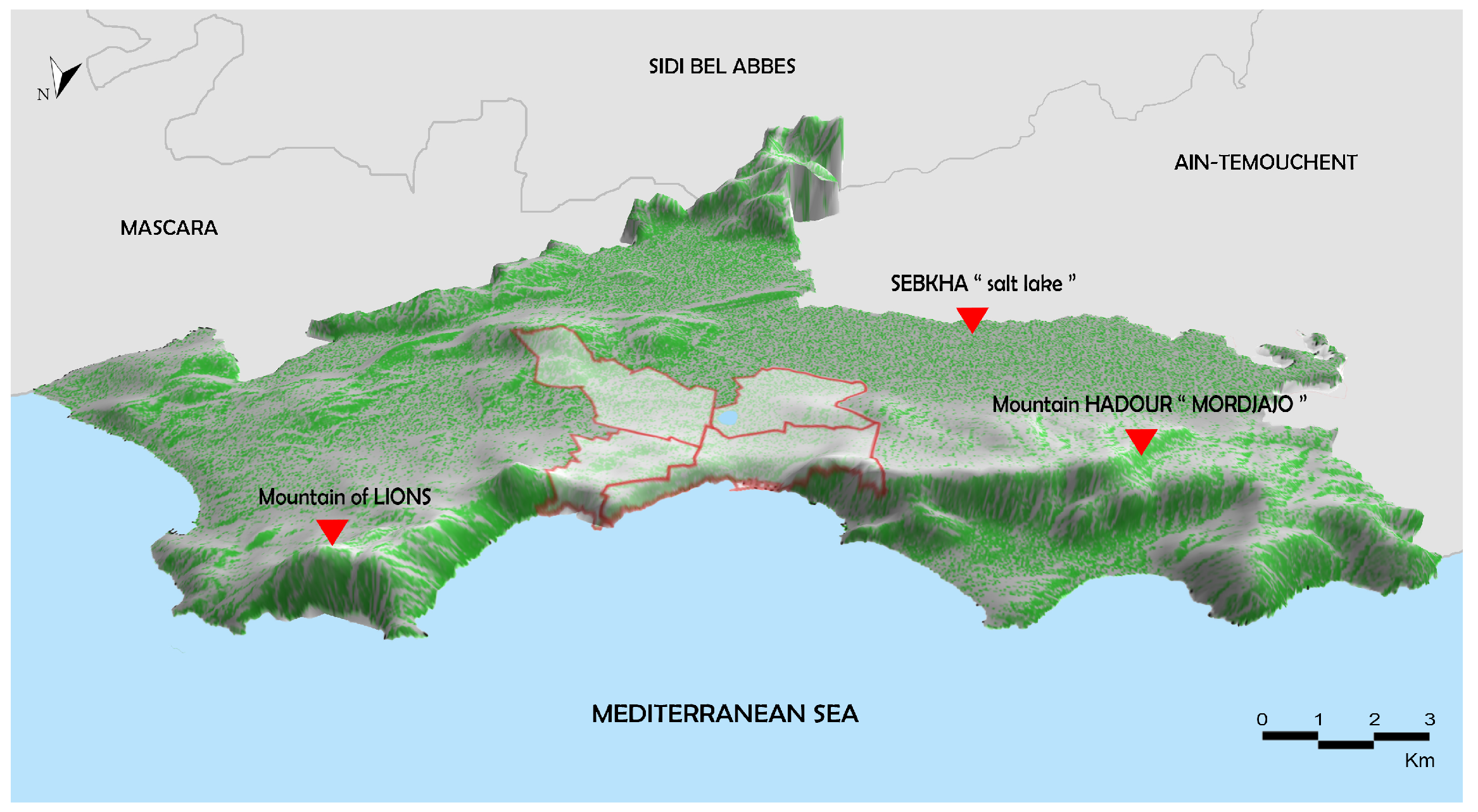
2.1. Study Area

Oran is a coastal city located in the Mediterranean Basin, in the northwest of Algeria, nestled at the head of a bay opening onto the Gulf of Oran, with a coastline approximately 70 km in length. It is situated between latitudes ${35}^{\circ }{40}^{\prime }$ N and ${35}^{\circ }{43}^{\prime }$ N, and longitudes $0^{\circ }{37}^{\prime }$ W [29] and $0^{\circ }{41}^{\prime }$ W. It is delimited to the east by the Mascara province, to the south by the Sidi Belabess province, and to the Ouset by the Ain-Temouchent province. As the country’s second-largest city and its economic capital, Oran covers an area of about 2121 km² [30] (Figure 2), while the region of interest represents $10.21\%$ of the total area of Oran, that is, about 216.63 km², and encompasses four municipalities: Oran, Bir El djir, Es Senia, and Sid Chahmi (Figure 2).

Figure 2. Oran location and the region of interest.

The city’s geography is marked by a varied topography, with an average altitude of 106 m. To the west, the Aïdour Mountain (or Murdjajo), which reaches an elevation of 429 m, forms a natural barrier, separating the municipality of Oran from that of Mers El-Kebir. The region’s minimum altitude is −2 m, found in areas below sea level, such as Sabkha (the lake) to the south, which is often prone to flooding or covered with salts. The maximum altitude is 507 m, located in the surrounding hills and mountains [31]—see Figure 3. The climate of Oran exhibits the typical characteristics of a Mediterranean climate, with an average annual temperature of approximately 18 °C [32]. Winters are generally mild, while summer temperatures can reach highs of up to 43 °C. Precipitation is concentrated during the wet season, from September to April, with an annual total of approximately 380 mm [32]. This Mediterranean climate significantly influences the local ecosystem as well as the socio-economic dynamics of the city, particularly in terms of urbanization and the lifestyle of its inhabitants. The city’s appeal to both domestic and international migrants has been a major driver of its population growth. The population increased from 750,000 in 2008 [33] to approximately 1.24 million in 2023, with nearly 90% of the population living in urban areas, compared to only 10% in rural zones, reflecting the rapid evolution of the urban landscape [33].

Figure 3. The geographical configuration of our study area.

In this work, Oran was chosen as the study area due to its accelerated urban growth and the intensive development of key industrial sectors such as construction, energy, and transport, which significantly impact the rise in urban temperatures. The reduction of green spaces and natural areas, often replaced by artificial infrastructure, further amplifies the city’s vulnerability to extreme weather events, exacerbating the environmental challenges associated with urbanization. Therefore, analyzing LST and the UHI effect is essential for understanding the thermal dynamics of the city and, hence, thinking of appropriate solutions.

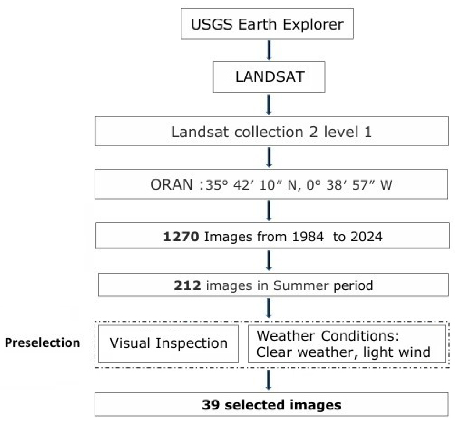
2.2. Landsat Imagery

Remote sensing is frequently used to analyze UHIs by measuring LST and studying the evolution of urban areas. Satellite data, such as those from Landsat, enable the monitoring of land cover changes and the identification of areas most vulnerable to thermal phenomena. Due to their extensive temporal coverage, Landsat data series play a crucial role in analyzing urban dynamics, their evolution, and the associated impacts, particularly with regard to rising urban temperatures [17,34]. Since its launch in 1972, the Landsat series has provided medium-resolution remote sensing data spanning over five decades. Landsat 5 TM features seven spectral bands, including one thermal infrared band (band 6). Landsat 7 ETM+ includes six reflective bands with a spatial resolution of 30 m, along with thermal infrared band (channels 6.1 and 6.2), with enhanced accuracy for LST determination using channel 6.2. Landsat 8 OLI/TIRS offers nine reflective bands and two thermal infrared bands (bands 10–11). Landsat 9, launched in 2021, further improves these capabilities with the TIRS-2. Although the native spatial resolution of the thermal bands varies (120 m for Landsat 5, 60 m for Landsat 7, and 100 m for Landsat 8/9), the data are published at a uniform spatial resolution of 30 m by the USGS [35]. A summary of the spectral bands used in this study is provided in Figure 4 [36].

Figure 4. Comparison of Landsat spectral bands [36].

2.3. Data Resources

For this study, we utilized Level 1 images from Landsat Collection 2, accessible through the Earth Explorer platform of the United States Geological Survey (USGS) [29]. A total of 1270 images, acquired from the Landsat 4–5, Landsat 7, and Landsat 8–9 satellites, covering the study area, were collected from the period between 1 January 1984 and 1 October 2024. However, only 212 images acquired during the summer period (from 21 June to 21 September) were selected. This period is characterized by an intensification of the UHI effect, due to the long duration of daylight hours and the increased solar radiation absorbed by urban surfaces. To ensure the accuracy of the results, images affected by cloud cover were systematically excluded. Although advanced cloud correction techniques are available in the literature, these were beyond the scope of the present study. Additionally, a selection of days with favorable meteorological conditions for studying the phenomenon, such as high atmospheric pressure, clear skies, and low synoptic winds [37], was made. This resulted in the retention of 39 images: six for June, seventeen for July, fourteen for August, and two for September. The selection procedure is illustrated in Figure 5.

Figure 5. Flowchart illustrating the image selection process.

Meteorological data necessary for the analysis were obtained from the Oran/Es Senia Weather Station [38], which provided detailed hourly data. These data were used to complement and refine the interpretation of the LST results. A complete list of all the satellite images analyzed is provided in Table 1.

Table 1. Selected images for the study.

Satellite	Acquisition Year	Total Image Count	Candidate Images Count	Selected Images After Meteorological Conditions Verification and Visual Inspection				Used Images
				Day/Month	Time (UTC)	T (°C)	Tmax (°C)
Landsat 5 (TM)	1984	504	4	28/07	10:07:24	25	28	1	15
	1985		6	31/07	10:08:02	26	29	1
	1986		6	03/08	10:00:19	27	29	1
	1987		5	07/09	10:04:53	27	29	1
	1988		6	24/08	10:09:00	27	31	1
	1989		5	26/07	10:05:24	27	29	1
	1990		6	14/08	09:58:12	29	35	1
	1991		5	01/08	10:01:42	26	29	1
	1992		5	03/08	10:01:00	26	28	1
	1993		5	07/09	10:00:35	25	30	1
	1994		5	25/08	09:55:18	28	34	1
	1995		6	27/07	09:42:31	30	34	1
	1996		6	27/06	09:51:41	25	29	1
	1997		6	01/08	10:09:16	26	29	1
	1998		5	19/07	10:16:31	27	30	1
Landsat 7 (ETM+)	1999	414	5	15/08	10:31:05	26	30	1	12
	2000		5	01/08	10:29:24	27.7	32.4	1
	2001		6	20/08	10:27:02	29	33	1
	2002		5	06/07	10:26:39	26	29	1
	2003		0	no image available in summer				0
	2004		3	25/06	10:27:15	28.3	29	1
	2005		0	no image available in summer				0
	2006		2	17/07	10:28:00	26.6	31	1
	2007		4	21/08	10:28:13	26.7	30	1
	2008		2	06/07	10:27:44	30.6	35	1
	2009		2	23/06	10:28:38	28.5	30	1
	2010		2	12/07	10:31:27	24.6	29	1
	2011		2	16/08	10:31:38	29.2	32	1
	2012		5	17/07	10:33:02	27	31	1
Landsat 8/9 (TIRS/OLI)	2013	352	6	07/28	10:40:13	28	32	1	12
	2014		6	29/06	10:37:58	29	32	1
	2015		6	18/07	10:37:48	28.6	31	1
	2016		5	05/08	10:38:15	34.2	36	1
	2017		6	21/06	10:37:58	25.3	28	1
	2018		6	08/06	10:37:02	25.5	27	1
	2019		6	14/08	10:38:21	27.8	30	1
	2020		6	31/07	10:38:10	28.5	32.6	1
	2021		6	02/07	10:38:07	27.3	30	1
	2022		11	29/07	10:38:15	28.8	32	1
	2023		12	08/07	10:37:54	29.6	30	1
	2024		12	10/07	10:37:37	28.2	33.6	1
Total	41 years	1270	212					39

2.4. Methodology

In our study, the methodology illustrated in Figure 6 was applied. We used 39 Landsat images, which were preprocessed and processed using MATLAB R2022. This allowed for the extraction of biophysical indices, particularly the NDBI, to identify built and non-built areas. To refine LULC data and analyze urban sprawl, a semi-automatic classification was performed using QGIS software version 3.10.5. Additionally, the NDVI was calculated to analyze vegetated areas, and it was further used to generate LST maps, which helped to estimate the intensity of the SUHI and assess its spatiotemporal evolution. The areas affected by UHI were identified, cross-referenced, and delineated, facilitating the determination of zones impacted by PUHI.

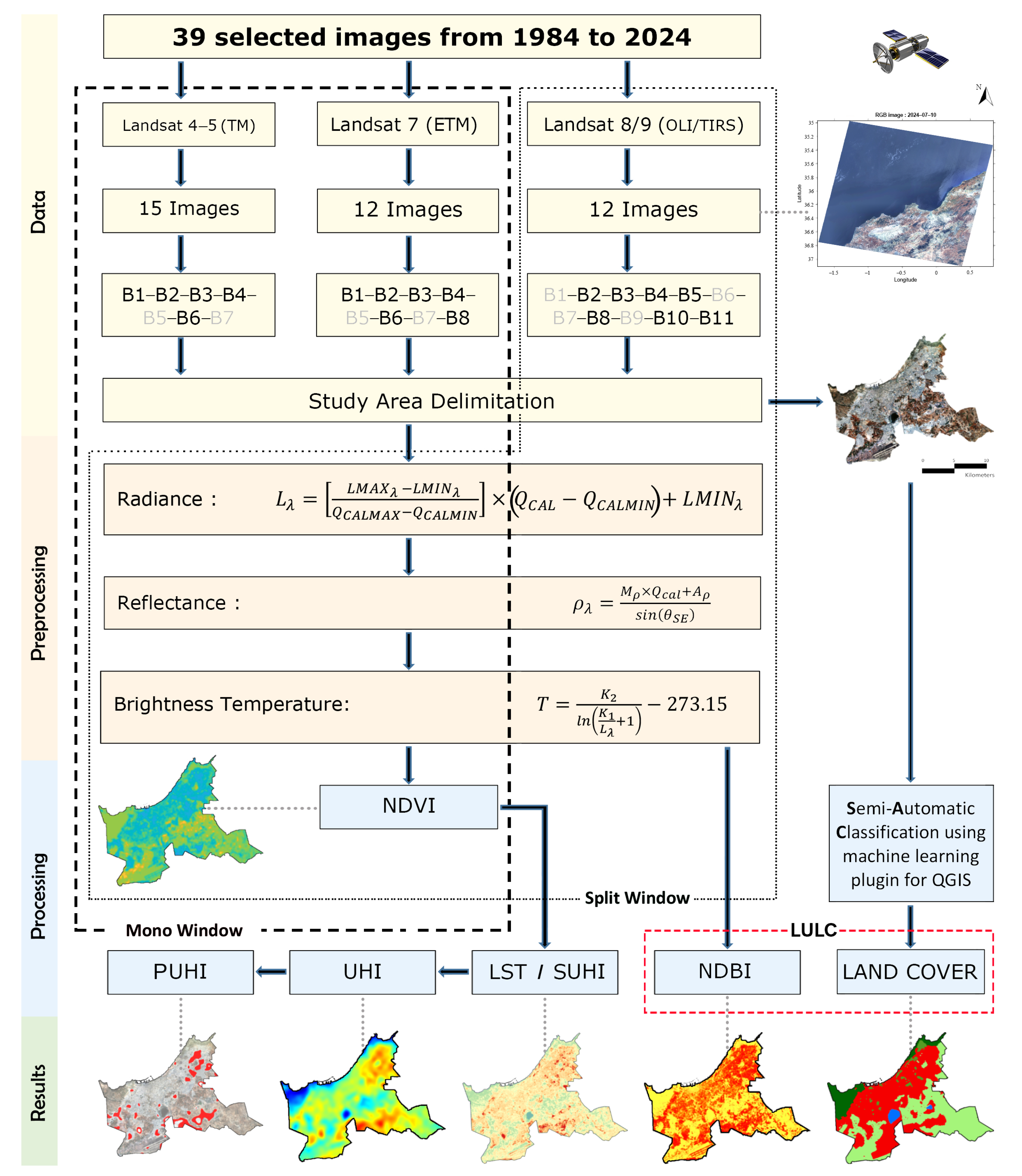
Figure 6. Flowchart of the methodology.

3. Pre-Processing

The images acquired by Landsat sensors may be affected by various distortions caused by the atmosphere, topography, and solar conditions, as well as the sensors themselves, which can compromise the accuracy of measurements [39]. Among these distortions, absorption and scattering are particularly significant, resulting from the interaction of electromagnetic radiation with atmospheric particles such as water vapor and aerosols [35]. These phenomena can undermine the quality of the data, especially for applications that require high radiometric precision, such as LST estimation. To ensure reliable results, preprocessing is essential to mitigate these biases and improve the overall quality of the images. In the context of this study, preprocessing was applied to the 39 selected images. This involved key steps such as radiometric calibration and atmospheric correction. Radiometric calibration converts the Digital Numbers (DN) of the pixels into physical units like radiance and reflectance, ensuring consistency across the dataset. Meanwhile, atmospheric correction minimizes the effects of absorption, scattering, and atmospheric haze by adjusting pixel values according to dark-pixel reference points in the image. These steps are crucial for obtaining precise and reliable measurements from remote sensing data [40].

3.1. Step 1: Radiance Calculation

The data obtained from Landsat sensors are initially represented as DN, within a range of 0 to 255 for Landsat 5–7 and 0 to 65,536 for Landsat 8–9. However, for meaningful interpretation in geospatial analyses, these values must be converted into physical quantities, such as spectral radiance Top Of Atmospheric (TOA). To aid in this conversion, each Landsat image is accompanied by a metadata file containing the relevant radiometric calibration coefficients [36]. This calibration process is essential to ensure the accuracy of the data and their alignment with the actual physical conditions observed on the ground, thus enabling their reliable application in remote sensing and environmental modeling.

• Landsat 5–7 at-sensor radiance:
  The radiance for Landsat 5 and 7 is calculated using Equation (1) [41]:

  $$L_{\lambda }={\displaystyle \frac{LMA{X}_{\lambda }-LMI{N}_{\lambda }}{Q_{CALMAX}-Q_{CALMIN}}}\times (Q_{CAL}-Q_{CALMIN})+LMI{N}_{\lambda },$$

  (1)

  where
  • $L_{\lambda }$ is the spectral radiance at the sensor aperture (Watts/(m².srad.μm));
  • $Q_{CAL}$ is the digital number;
  • $Q_{CALMAX}$ and $Q_{CALMIN}$ refer to the maximum and minimum quantized calibrated pixel value;
  • $LMA{X}_{\lambda }$ refers to spectral radiance scales to $Q_{CALMAX}$;
  • $LMI{N}_{\lambda }$ refers to spectral radiance scales to $Q_{CALMIN}$.
• Landsat 8–9 at-sensor radiance:
  Equation (2) presents the formula used to converting DN to spectral radiance on Landsat 8 and 9 [41]:

  $$L_{\lambda }=M_{\lambda }\times Q_{CAL}+A_{\lambda },$$

  (2)

  where
  • $L_{\lambda }$ is the spectral radiance at the sensor aperture (Watts/(m².srad.μm));
  • $A_{\lambda }$ represents the band-specific additive rescaling factor;
  • $M_{\lambda }$ represents the band-specific multiplicative rescaling factor from the metadata;
  • $Q_{CAL}$ represents the quantized and calibrated standard product pixel values DN.

3.2. Step 2: The Surface Reflectance Calculation

Surface Reflectance (${\rho }_{\lambda }$) measures the fraction of incoming solar radiation that is reflected from Earth’s surface to the Landsat sensor [42]. To calculate ${\rho }_{\lambda }$, we use the following equation:

$${\rho }_{\lambda }={\displaystyle \frac{M_{\rho }\times Q_{CAL}+A_{\rho }}{sin\left({\theta }_Z\right)}},$$

(3)

where

• $M_{\rho }$: reflectance multiplicative scaling factor;
• $A_{\rho }$: reflectance additive scaling factor;
• $Q_{CAL}$: pixel value in DN for the band;
• ${\theta }_Z=90-\theta$, where $\theta$ is the local solar elevation angle.

3.3. Step 3: The Brightness Temperature Calculation

After converting the DN values to spectral radiance at the sensors surface, the TIRS bands data must be converted to Brightness Temperature (BT) using the thermal constants provided in the metadata file and Equation (4); the temperature is expressed in degrees Celsius [41]:

$$BT={\displaystyle \frac{K_2}{ln\left(\frac{K_1}{L_{\lambda }}+1\right)}}-273.15,$$

(4)

where

• $BT$ stands for brightness temperature (°C);
• $K_1$, $K_2$ are the calibration constants, reported in Table 2;
  Table 2. Thermal constant ($K_1$, $K_2$) values for Landsat (TM, ETM+, OLI, and TIRS).

  Satellite	K1 (watts/(m2.srad.μm))	K2 (Kelvin)
  Landsat 5 (band 6)	607.76	1260.56
  Landsat 7 (band 6)	666.09	1282.71
  Landsat 8 (band 10)	774.89	1321.08
  Landsat 8 (band 11)	480.89	1201.14
  Landsat 9 (band 10)	799.03	1329.24
  Landsat 9 (band 11)	475.66	1198.35

• $L_{\lambda }$ refers to the spectral radiance obtained from Equations (1) or (2).

4. Processing

4.1. The Normalized Difference Vegetation Index Calculation

The NDVI is a key indicator for assessing urban climate and vegetation cover. It ranges from $-1$ to $+1$ [43], where high positive values (close to $+1$) indicate a high presence of vegetation, low positive values correspond to bare soil or built-up areas, and values approaching zero or negative values (close to $-1$) are associated with water bodies. NDVI provides essential information about vegetation abundance, phenology, and health. This index is computed using the red ($RED$) band (0.6∼0.7 μm) and the near-infrared ($NIR$) band (0.7∼1.3 μm), according to Equation (5) [44].

$$\mathrm{NDVI}={\displaystyle \frac{NIR-RED}{NIR+RED}},$$

(5)

where $NIR$ band represents Band 4 in Landsat 5–7 and Band 5 in Landsat 8–9. The $RED$ band represents Band 3 in Landsat 5–7 and Band 4 in Landsat 8–9. The calculation of NDVI is necessary to further calculate the Proportion of Vegetation ($P_v$) and Emissivity $\left(ϵ\right)$.

4.2. The Normalized Difference Built-Up Index Calculation

The NDBI serves as a key indicator for urban climate analysis and the delineation of built-up areas. Compared to other land cover types or vegetation, urbanized zones exhibit higher reflectance in the mid-infrared (MIR) wavelength range (1.55∼1.75 μm) than in the near-infrared ($NIR$) range (0.76∼0.90 μm). The NDBI values range from $-1$ to $+1$, with high values indicating urbanized areas, low positive values corresponding to bare soils, and negative values signifying water bodies or vegetation. This index provides valuable insights into the extent of soil impermeability. The NDBI is derived using Equation (4) from the $NIR$ and $MIR$ bands [45,46]:

$$\mathrm{NDBI}={\displaystyle \frac{MIR-NIR}{MIR+NIR}},$$

(6)

where

• $MIR$ represents Band 5 in Landsat 5–7 and Band 6 in Landsat 8–9;
• $NIR$ represents Band 4 in Landsat 5–7 and Band 5 in Landsat 8–9.

4.3. Calculate the Proportion of Vegetation

Different types of land cover can be detected through the $P_v$ factor, where the vegetation and bare soil proportions are derived from the NDVI values of so-called “pure” pixels. To calculate the $P_v$, the following equation was used [20]:

$$P_v={\left({\displaystyle \frac{NDVI-NDV{I}_s}{NDV{I}_v+NDV{I}_s}}\right)}^2,$$

(7)

where

• $NDV{I}_v=0.5$ represents the vegetated surfaces;
• $NDV{I}_s=0.2$ represents the bare soils.

However, the $NDV{I}_v$ value may change in some cases; thus, for high-resolution data, particularly over agricultural sites, $NDV{I}_v$ can reach 0.8 or even 0.9 [20,42].

4.4. Calculate the Land Surface Emissivity

For the estimation of LST, the Land Surface Emissivity (LSE) must be calculated. The LSE serves as a proportionality factor that scales the black-body radiance (according to Planck’s law) to measure the emitted radiance. It represents the surface’s ability to transmit thermal energy to the atmosphere [21]. The LSE is largely influenced by factors such as surface roughness, the nature of vegetation cover, and other variables. The emissivity of water bodies is very stable in comparison with land surfaces. Since the emissivity depends on the wavelength, the NDVI Threshold Method (NTM) can be used to estimate the emissivity of different land surfaces in the (10∼12 μm) range. The emissivity is given by Equation (8) [20,21,41]:

$${ϵ}_{\lambda }=\left\{\begin{array}{cc}{ϵ}_s,\hfill & NDVI<NDV{I}_s\hfill \\ {ϵ}_s{P}_v+{ϵ}_s(1-P_v)+c,\hfill & NDV{I}_s\le NDVI\le NDV{I}_v\hfill \\ {ϵ}_s+c,\hfill & NDVI>NDV{I}_v\hfill \end{array}\right.$$

(8)

where ${ϵ}_v=0.5$ and ${ϵ}_s=0.2$ are the vegetation and soil emissivity, respectively, and c is the surface roughness, taken as a constant value of 0.005.

5. LST Estimation

Several approaches have been published for extracting LST using thermal remote sensing. A review of these methods can be found in works [19,21,45], among others. These algorithms include Single Channel (SC), Dual Angle (DA), Mono-Window (MW), and Split Window (SW). For our study, the MW and SW algorithms were selected for LST estimation.

5.1. The Mono-Window Algorithm

To estimate LST, designed for the TM6 sensors on the Landsat satellite, the MW algorithm was developed by Qin et al. [20]. This algorithm is based on two key concepts: a single spectral window and a simplified atmospheric model. To avoid reliance on radiosonde data in the Radiative Transfer Equation (RTE) method, the algorithm uses a single thermal band (hence the term “mono window”) to estimate LST, thereby simplifying the calculations. Surface temperature is then estimated from the radiance measured by the sensor, the surface emissivity, and the atmospheric temperature through an empirical relationship, the calculation of which is carried out using Equation (9), provided below [20].

$$T_s={\displaystyle \frac{1}{C}}[a(1-C-D)+(b(1-C-D)+C+D)T_{\mathit{sensor}}-D{T}_a],$$

(9)

with $C=ϵ\tau$, $D=(1-\tau )[1+(1-ϵ\left)\tau \right]$, $a=-67.355351$, and $b=0.458606$, and where $ϵ$ is the LSE, $\tau$ is the total atmospheric transmissivity, $T_{\mathit{sensor}}$ is the at-sensor BT, and $T_a$ represents the mean atmospheric temperature, given by

$$T_a=16.0110+0.92621T_0,$$

(10)

where $T_0$ is the near-surface air temperature. The atmospheric transmissivity is estimated from the atmospheric water vapor content w, for the range 0.4∼1.6 g/cm ², according to [21]

$$\begin{array}{cc}\hfill \tau =0.974290-0.08007w& (\mathrm{for}\mathrm{high}{T}_0)\hfill \end{array}$$

(11a)

$$\begin{array}{cc}\hfill \tau =0.982007-0.09611w& (\mathrm{for}\mathrm{low}{T}_0)\hfill \end{array}$$

(11b)

5.2. The Split-Window Algorithm

The Split-Window (SW) algorithm is based on the differential atmospheric absorption between two radiometric channels in the infrared window region, ranging from 10 to 12.5 μm. Initially designed to produce real-time sea surface temperature maps for oceans and water bodies, this algorithm assumed that the surface acted as a black body. However, subsequent studies showed that the SW algorithm minimizes the impact of surface emissivity, and that a slight overestimation of atmospheric water vapor absorption could compensate for this effect within a reasonable range of atmospheric water vapor content [22,47]. The algorithm calculates LST by applying a linear or nonlinear combination of the BT from the two adjacent infrared channels. Not requiring precise atmospheric profile data at the time of measurement, several variants have been developed to estimate LST from different sensors. The mathematical formula used to estimate LST can be formulated as [22]

$$T_s=T_i+c_1(T_i-T_j)+c_2{(T_i-T_j)}^2+c_0+(c_3+c_{4}w)(1-ϵ)+(c_5+c_{6}w)\Delta ϵ,$$

(12)

where

• $T_s$ represents the land surface temperature;
• $T_i$, $T_j$: at-sensor BT of the SW bands i and j in Kelvin;
• w: the atmospheric water vapor content;
• $ϵ$: the mean emissivity;
• $\Delta ϵ$: the emissivity difference;
• $c_i$ are coefficients, given in Table 3.
  Table 3. Split-window coefficient values.

  Constant	${\mathit{c}}_0$	${\mathit{c}}_1$	${\mathit{c}}_2$	${\mathit{c}}_3$	${\mathit{c}}_4$	${\mathit{c}}_5$	${\mathit{c}}_6$
  Value	$-0.268$	1.378	0.183	54.300	$-2.238$	$-129.200$	16.400

6. Estimation of Surface Urban Heat Island

According to the literature, there are four main methods for estimating the Surface Urban Heat Island (SUHI) [48]. The first method, statistical models, such as the Gaussian Surface Model (GSM) and the kernel convolution method, are used to quantify and model SUHI based on various parameters, such as the spatial distribution of temperatures. The second method, the LST/BT classification method, involves classifying UHIs using LST or BT images, thereby allowing for a better identification of SUHI distribution. The third method, the UHI Index (Heat Island Index), relies on four key indicators: UHI Ratio Index (URI), Urban Thermal Field Variance Index (UTFVI), Maximum UHI Index (MUI), and Weighted Average UHI Index (WAUI), which help to analyze and quantify the intensity of UHIs. Finally, the fourth method, the temperature dichotomy method, determines SUHI by measuring the temperature difference between urban and rural areas simultaneously. It uses the following equation [7,49,50]:

$$\mathit{SUHI}=LS{T}_{\mathit{urban}}-LS{T}_{\mathit{rural}},$$

(13)

where the $LS{T}_{\mathit{urban}}$ and $LS{T}_{\mathit{rural}}$ values represent the average temperature of the pixels within the urban and rural area, respectively. This last method was used to calculate and quantify the SUHI in our study.

7. Results and Discussion

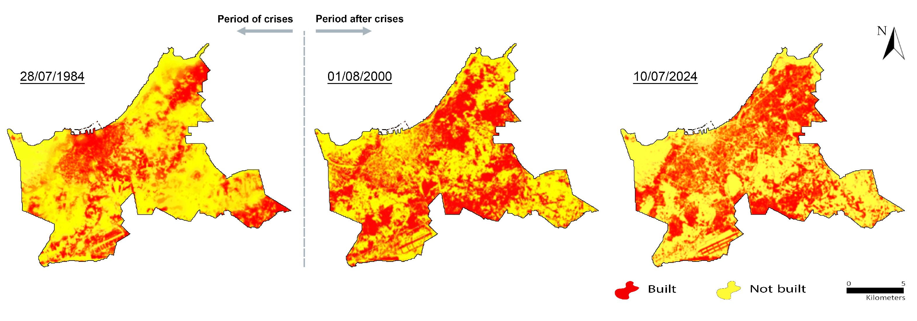
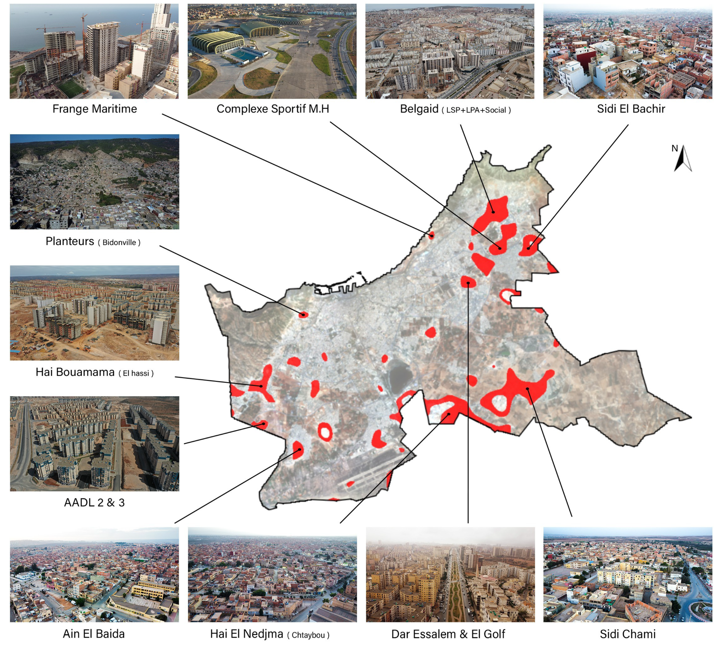
7.1. Land Cover Analysis

In the context of analyzing the urban evolution of the city of Oran between 1984 and 2024 and identifying built-up areas, we initially applied the NDBI using Landsat satellite imagery from 28 July 1984, 1 August 2000, and 10 July 2024. This served as an initial step for the preliminary detection of urban zones. However, leveraging our knowledge of the terrain, we could identify certain inaccuracies in the results presented in Figure 7. Specifically, several areas that are not built-up were mistakenly classified as urban, including rocky regions. This observation prompted the use of the Semi-automatic Classification Plugin (SCP), integrated into QGIS software, to obtain more precise results. Developed in 2012 as part of the “Adapting to Climate Change in Coastal Dar es Salaam” (ACC Dar) project by Congedo [51], this open-source tool was employed to classify urban areas, refine initial results, and improve the accuracy of the analysis. By combining these methods, a more precise maps of Oran’s urban expansion and land cover was generated, as illustrated in Figure 8. We can distinguish two principal periods:

• Between 1984 and 2000: The political and economic crisis of the 1980s and 1990s in Algeria, coupled with significant demographic pressure, exacerbated the housing deficit. In response, several reforms were implemented, including the promulgation of the law on municipal land reserves, the adoption of regulatory texts for operational urban planning, and the 1981 sale of state-owned properties [33]. These reforms gave rise to the development of peripheral neighborhoods, such as USTO, Akid Lotfi, Ain Baida, Hai Bouamama (El Hassi), and Hai El Wiam (Sidi El Bachir)—see Figure 8;
• Between 2000 and 2024: Following the end of the political and economic crisis, the city experienced a notable revival in housing and construction programs, driven by the implementation of national initiatives, such as the following [28]:

  -

  The Participatory Social Housing ‘2001’, primarily benefiting the Hai Essabah and USTO neighborhoods;

  -

  The Public Rental Housing ‘2001’, deployed in the USTO, Hai Bouamama (El Hassi), and Ain Baida districts;

  -

  The Assisted Promotional Housing ‘2013’, concentrated in the the Belgaid and Es-Senia neighborhoods;

  -

  The Public Promotional Housing ‘2016’, mainly located in the El Barki area;

  -

  Social programs implemented in different peripheral neighborhoods.

  These policies triggered significant urban transformation, fostering pronounced urban sprawl, particularly towards the eastern part of the city.

Figure 7. Normalized Difference Built-up Index (NDBI), from 1984 to 2024.

Figure 8. Land Use/Land Cover (LULC) use between 1984 and 2024.

This rapid urbanization is clearly reflected in the data on the evolution of urban areas in Oran. The extent of urban zones increased from $21.6\%$ in 1984 to $51.83\%$ in 2024, marking a $30.23\%$ increase, with the land area growing from 46.78 km² to 112.06 km² (see Figure 9). The most substantial development occurred between 2000 and 2024, with an increase of 42.12 km², representing a growth of $19.50\%$, coinciding with the implementation of various state-supported housing programs, as mentioned earlier. In contrast, the most notable decrease concerns agricultural land, which shrank from $66.86\%$ in 1984 to $38.73\%$ in 2024 (60.80 km², a $28.13\%$ decline), representing a reduction in agricultural area from 144.54 km² to 83.74 km². This phenomenon is not unique to Oran, as similar trends can be observed in other Mediterranean cities, such as Granada (Spain), where urban areas increased by $7\%$ between 1985 and 2020 [50,52]. Thus, the urban sprawl observed in Oran reflects a broader pattern seen in several Mediterranean cities, highlighting the scale of urban landscape transformation in the region over the past few decades.

Figure 9. Changes in urban areas and land cover types from 1984 to 2024.

7.2. Spatiotemporal Distribution of NDVI Between 1984 and 2024

The NDVI maps for the city of Oran for the years 1984, 2000, 2010, 2020, and 2024 are presented in Figure 10, and their descriptive statistics are summarized in Table 4. The results indicate that NDVI values ranged from $-0.15$ to $0.36$ throughout the study period. To analyze these variations, a classification into four distinct classes was established. The first class, corresponding to an NDVI lower than 0.00, represents water bodies. The second class, with an NDVI ranging from 0.00 to 0.13, is associated with urban areas and impermeable surfaces. The third class, with an NDVI between 0.13 and 0.22, represents agricultural lands. Finally, the fourth class, corresponding to an NDVI greater than 0.22, is attributed to vegetation. This classification allows for the identification and a better understanding of the spatial distribution of different land covers and their evolution in the city of Oran over the years.

Figure 10. Normalized Difference Vegetation Index (NDVI) from 1984 to 2024.

Table 4. Classification based on NDVI.

Class	NDVI	Area	1984	2000	2010	2020	2024
Water	<0	km2	0.17	0.79	0.17	1.41	0.05
		%	0.08	0.36	0.08	0.65	0.02
Urban and rock	0–0.13	km2	45.30	66.41	87.41	92.35	107.67
		%	20.91	30.66	40.35	42.63	49.70
Agriculture	0.13–0.22	km2	139.76	118.33	101.83	96.54	79.94
		%	64.52	54.63	47.01	44.57	36.90
Vegetation	>0.22	km2	31.39	31.09	27.21	26.33	28.97
		%	14.49	14.35	12.56	12.16	13.37

Table 4 indicates that, in 1984, the area of agricultural land associated with vegetated surfaces was 171.15 km², representing $79\%$ of the total area. In 2000, this area decreased to 149.42 km², or $69\%$, with an average annual reduction of approximately $0.63\%$. By 2024, it further declined to 108.91 km², representing $50\%$ of the total area of interest. Over the entire study period, the average annual decrease was about $0.73\%$. Regarding the observed water surface variability, there are two significant areas representing salt lakes (Sebkha) in our study area, whose levels are influenced by heat and evaporation, which can lead to their complete drying up during certain periods.

The spatiotemporal analysis of the NDVI highlights changes in LULC in Oran and reveals an opposing development between urbanization and vegetation cover. It shows that urban expansion has led to a reduction in vegetated areas, emphasizing the impact of urbanization on the natural environment. This confirms the results obtained from the LULC analysis.

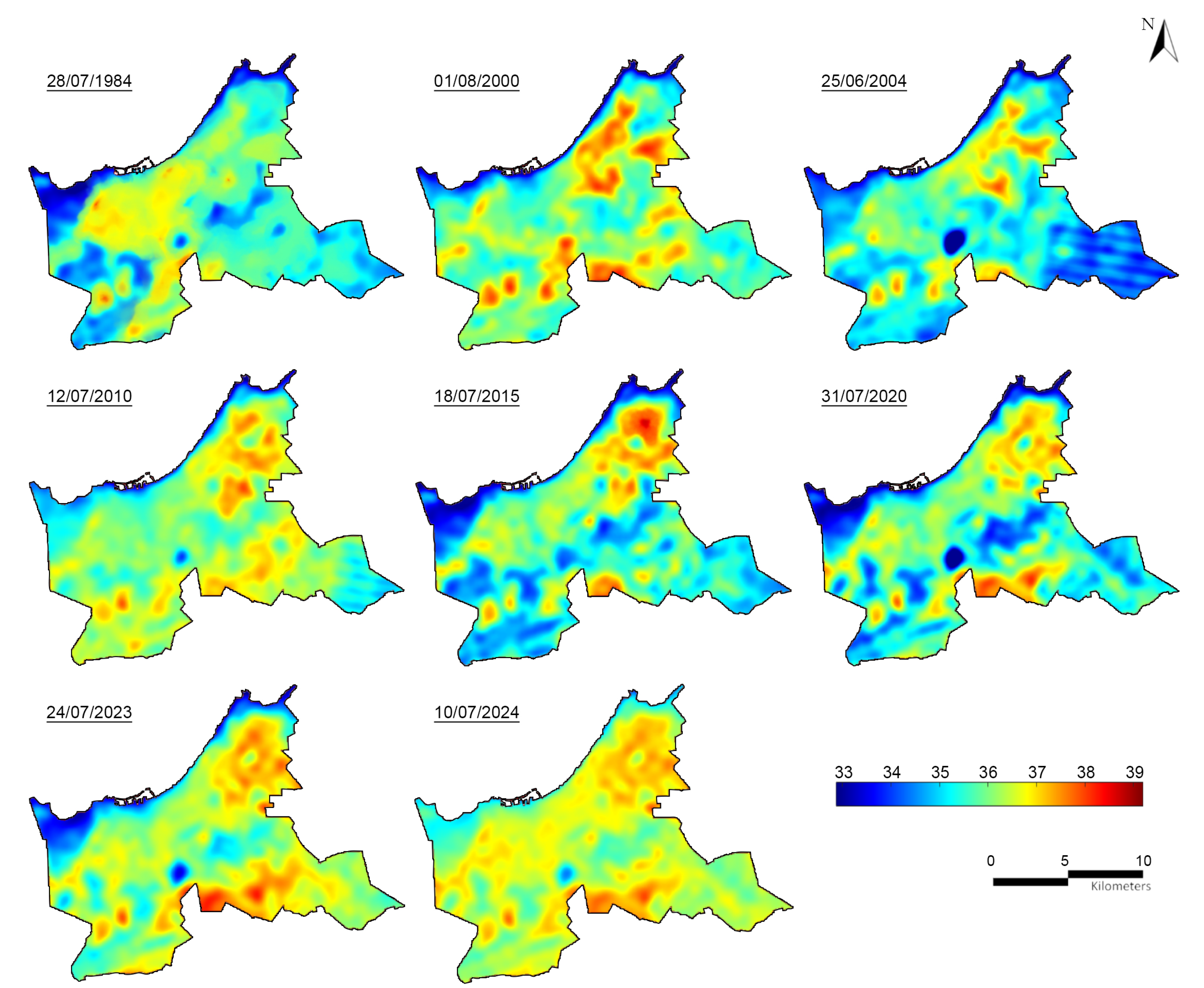
7.3. Land Surface Temperature Distribution

The visual inspection of the LST results allowed for the identification of three distinct temperature categories (Figure 11). Figure 12 presents a graph of the data from Table 5, which includes the surface areas of the three thermal classes adopted in our analysis:

Figure 11. Spatiotemporal distribution of Land Surface Temperature (LST) in Oran.

Figure 12. Variability of the LST of Oran by year.

Table 5. LST classification area evolution, from 1984 to 2024.

LST	Area	1984	2000	2004	2010	2015	2020	2023	2024
<34 °C	km2	173.30	148.84	129.58	112.37	80.89	86.65	37.17	66.35
	%	80.16	68.85	59.94	51.98	37.42	40.08	17.19	30.69
35–41 °C	km2	42.49	66.19	85.20	102.39	133.54	128.70	174.40	147.67
	%	19.66	30.62	39.41	47.36	61.77	59.53	80.67	68.31
>42 °C	km2	0.40	1.16	1.41	1.43	1.77	0.85	4.62	2.17
	%	0.18	0.54	0.65	0.66	0.82	0.39	2.14	1.00

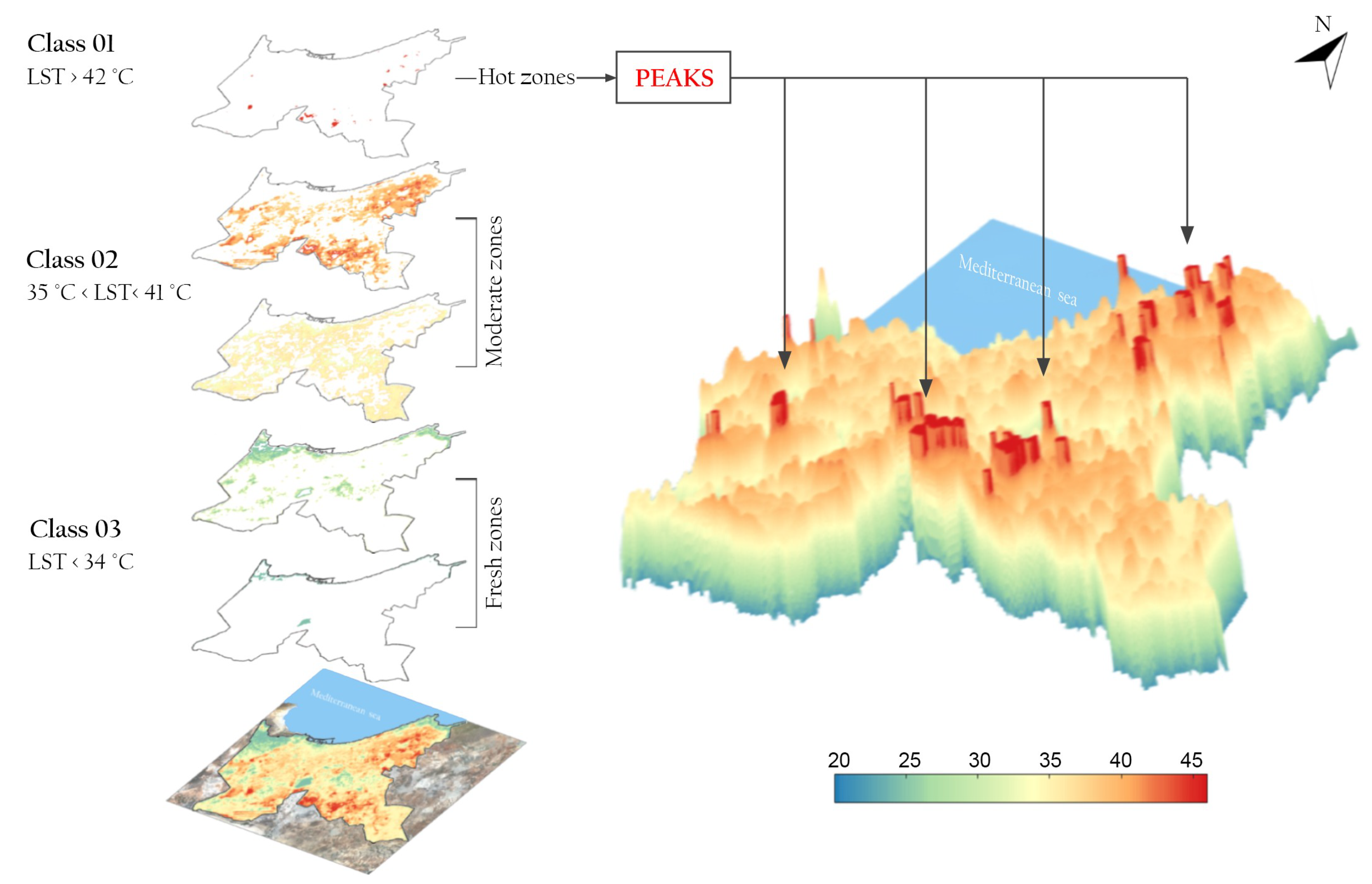
• Class 1 includes areas with temperatures below 34 °C, classified as cool zones. These areas correspond to non-urbanized regions, rural regions such as vegetated soils, natural terrains, water bodies, and the coastal strip. However, these areas have undergone regression due to the urban sprawl experienced by Oran, as shown by the results in the table. Indeed, the affected area was 173.30 km², accounting for $80.16\%$ of the total study area (216 km²) in 1984. This area has decreased over the following decades, dropping to 148.84 km² in 2000 ($68.85\%$) and to 66.35 km² in 2024 ($30.69\%$), reflecting an average annual reduction of approximately 6.76 km²;
• Class 2 includes areas with temperatures ranging from 35 °C to 41 °C, classified as moderate zones. These areas primarily correspond to the historic city center of Oran, a legacy of urban development dating back to the colonial period, including neighborhoods such as Sidi Houari, Miramar, St Pierre, and Gambetta, as well as the peri-urban areas of the city. Unlike Class 1, this class has experienced a significant expansion, with an average annual increase of about 5.07 km², directly resulting from the urban sprawl of the city and its outskirts. In 1984, the corresponding area was 42.49 km², representing 19.66 % of the total studied area. This area has gradually expended over the decades, reaching 66.85 km² in 2000 (30.62 %) and 147.67 km² in 2024 (68.31 %);
• Class 3 refers to areas where surface temperatures exceed 42 °C, representing the peaks of surface temperatures and designated as hot zones (Figure 13). These zones can be primarily located in four distinct areas:
  

  Figure 13. LST classification corresponding to 24 July 2023.

  -

  Zone 1 (circle 2 in Figure 11A) encompasses one of the largest informal settlements, “Les Planteurs”, located to the west of the city. It is characterized by chaotic urbanization and the construction of buildings from salvaged materials. These precarious constructions, using materials unsuitable for heat, such as corrugated metal roofing and plastic tarps for waterproofing, also suffer from a lack of ventilation and green spaces. This zone also includes the Bouamama “El Hassi” neighborhood, where urbanization is marked by unfinished buildings, predominantly with concrete roofs and brick and cinder block walls. A part of this neighborhood is also occupied by a slum, exacerbating the precarious living conditions;

  -

  Zone 2 (circle 3 in Figure 11A) covers the Senia industrial area, located to the south of the city, dominated by metal structures and administrative buildings with glass facades (curtain walls), which contribute to heat accumulation, exacerbated by industrial activities and high energy consumption. It also includes the neighborhoods of Hai Nejma (Chataybou) and Sid Echahmi, which emerged in the 1990s, characterized by incomplete urban structures and unfinished buildings, primarily with exposed brick facades;

  -

  Zone 3 (circle 4 in Figure 11A) corresponds to the eastern part of Oran, where urban expansion has been particularly pronounced due to physical barriers such as the Mediterranean Sea to the north, the Murdjadjo mountain to the west, and the Sebkha (salt lake) to the south. This zone houses several neighborhoods, including Hai Sabah, Hai El Yasmine, and Belgaïd, which have benefited from significant housing programs such as LSP, LPA, and AADL1, as well as social housing and LPP. However, this expansion continues to grow with significant urban densification, widespread concreting, and a lack of green spaces. The neighborhoods continue to expand, with large-scale construction and earthworks ongoing. Furthermore, major infrastructures such as the Miloud Hadfi sports complex (built for the 2022 Mediterranean Games) and the Abou Bekr Belgaïd university complex complement this dynamic;

  -

  Zone 4 (circle 5 in Figure 11A) covers the southwestern part of the city, where AADL 2 and 3 housing programs have been added to an already poorly structured and inadequately planned area, Ain Bayda. This expansion has led to an increase in impermeable surfaces, thereby contributing to higher local temperatures and exacerbating the UHI effect.

  For this class, the area was 0.4 km² in 1984, representing $0.18\%$ of the studied zone. This area has gradually increased, reaching 1.16 km² in 2000 ($0.54\%$) and 2.17 km² in 2024 ($1\%$), with an average increase of approximately 0.07 km² per year.

7.4. Correlation Between LST and NDVI

The relationship between LST and the NDVI was examined using linear regression correlation analysis. The correlation between these two variables is depicted in Figure 14. A random sample of 2500 points was selected, with NDVI values ranging from $-0.14$ to $0.4$. The results indicate a negative linear correlation between LST and NDVI, described by the equation $y=-0.24x+42$, with an inter-correlation coefficient of $-0.65$. This suggests that an increase in LST is associated with a decrease in NDVI, and vice versa this can be also confirmed by the work in [43]. Therefore, areas with reduced vegetation cover experience higher surface temperatures.

Figure 14. Linear regression between LST and NDVI.

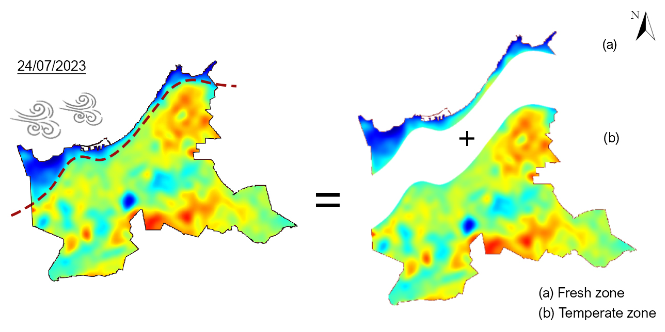
7.5. Evolution of the SUHI in Oran (1984–2024): Spatiotemporal Analysis

The analysis of the evolution of the SUHI in Oran between 1984 and 2024 reveals four distinct phases, each marked by unique urban and climatic dynamics (Figure 15). From 1984 to 2000, SUHI exhibited moderate growth, with the temperature difference between urban and rural areas increasing from 0.36 °C to 1.7 °C, reflecting an average annual increase of 0.08 °C. This modest rise can be attributed to limited urbanization during this period, constrained by economic and political crises that slowed city expansion and infrastructure development. A significant shift occurred between 2000 and 2018, characterized by a rapid intensification of SUHI, particularly in the city’s eastern peripheries. By 2018, the temperature differential had surged to 5.28 °C, with an average annual growth rate of 0.24 °C, similar to trends observed within the Mediterranean basin, such as in Athens (0.21 °C), Marseille (0.60 °C), Barcelona (0.31 °C), and Rome (0.33 °C) [24]. This phase coincided with large-scale urban expansion driven by housing programs (e.g., LST, AADL, LPA, LPP) and infrastructure development. Population growth and urban densification further exacerbated the heat island effect, despite the presence of agricultural lands and vegetated areas that traditionally act as cooling elements. Between 2019 and 2021, a temporary decline in SUHI intensity was observed, with the temperature difference dropping from 4.43 °C in 2019 to 4.41 °C in 2020. This slight decrease can be linked to the effects of the COVID-19 pandemic, which curtailed human activities [53], contributing to a temporary attenuation of the UHI effect. From 2021 to 2024, SUHI resumed its upward trend following the lifting of pandemic restrictions and the resumption of urbanization projects. The 2022 Mediterranean Games spurred significant developments, particularly in the city’s eastern zones, including the construction of a Mediterranean village, sports facilities, and related infrastructure. This led to a peak SUHI intensity of 5.4 °C in 2023, coinciding with the hottest year globally recorded, exacerbated by an intense El Niño event. In 2024, a slight regression was observed, with SUHI declining to 4.5 °C, indicating a modest relative decline in contrast to global climatic trends.

Figure 15. Surface Urban Heat Island (SUHI) evolution from 1984 to 2024.

7.6. Spatiotemporal Evolution of Urban Heat Islands in Oran (1984–2024)

To map the UHIs, the application of Equation (14) [50] allowed the isolation of pixels corresponding to the highest LST, considered uncomfortable for human life and named as Urban Hotspots (UHSs). There areas are depicted in Figure 16.

$$LST>\mu +2\sigma ,$$

(14)

where $\mu$ represents the mean value and $\sigma$ denotes the standard deviation of the surface temperature (LST) within the study area, expressed in °C.

Figure 16. Urban Hotspot (UHS) variability in the studied area by year.

This method was applied to the years 1984, 2000, 2004, 2010, 2015, 2020, 2023, and 2024, enabling the identification of the first class, labeled “Very High”, which represents UHS, indicated by red patches on the maps (Figure 17), obtaned using Equation (14). An additional thresholding process was then employed to generate three complementary categories: “High Temperature”, “Moderate”, and ”Low”, as depicted in Figure 17. These categories enhanced the spatial mapping of UHIs, providing a valuable analytical tool to study their evolution over the specified years.

Figure 17. Spatiotemporal evolution of Urban Heat Island (UHI) in Oran.

The spatiotemporal dynamics of UHIs in Oran exhibit a similar trend to the SUHI already studied. “Very High” classified zones demonstrated significant growth, increasing from 2.1 km² (1984) to 13.32 km² (2024), with an annual average expansion of 1 km². A notable peak was recorded in 2023 (14.93 km²), coinciding with global warming trends. The COVID-19 pandemic induced a temporary reduction in UHI area (1.51 km²) between 2019 and 2020. By the analysis of the UHI maps of Oran city, another finding revealed a distinct spatial organization, characterized by two contrasting climatic zones. The first is a cooler zone, influenced by the sea breeze, corresponding to the coastal strip along the Mediterranean basin. This zone includes the lower part (level 00) of the city, encompassing the port, the new expressway linking Oran to the east–west highway, and a large portion of the old city center. In contrast, the second zone (level +50 m) is marked by significantly higher temperatures, spatially distributed differently, primarily in densely urbanized areas, as shown in Figure 18.

Figure 18. Distinct specialization of Oran.

7.7. Permanent UHI

The areas where UHI manifested permanently during the last decades are illustrated in Figure 19, which highlights several significant hotspots. Among these are the Belgaïd district, the coastal fringe, and the newly developed AADL neighborhoods, which are characterized by high-density, closely packed constructions and a notable lack of green spaces. The districts of Sidi El Bachir and Sidi Chahmi stand out due to their predominantly unfinished structures, often left in raw brick form. Additionally, the industrial zone of Haï Nejma Chtaybou, dominated by numerous metallic structures, represents another significant UHI hotspot. Lastly, the informal Planteurs neighborhood, where rooftops are predominantly made of corrugated metal, also contributes substantially to this phenomenon. Recent studies have highlighted that such stable PUHIs pose a greater danger to resident compared to general UHIs [52,54].

Figure 19. Permanent Urban Heat Island (PUHI) in Oran.

8. Conclusions

This study explores the changes in land use within the Oran region and its effects on the formation and intensification of UHI over the past 40 years, from 1984 to 2024, during the summer months. To achieve this, remote sensing data (LANDSAT images) and geographic information systems (GIS) were utilized to estimate LST and calculate biophysical indices such as the NDVI and the NDBI. These datasets enabled the identification, measurement, and analysis of both SUHI and UHI across the same time period.

The results indicated that areas with high surface temperatures are primarily located in urban zones, predominantly in the eastern part of Oran, where urban growth is most pronounced. This expansion is largely driven by land scarcity, aggravated by physical geographic barriers surrounding the city, such as the Mediterranean Sea to the north, the saline lake to the south, and the Mordjajo mountain range to the West. In contrast, lower temperatures are found in vegetated areas on the city’s periphery, which serve as cooler zones. Furthermore, this study highlights that the coastal strip of Oran along the Mediterranean is significantly cooler than the inner city regions. This cooler temperature is primarily attributed to the moderating effect of the sea breeze, which brings fresh, cool air along the coastline.

Ultimately, the complex relationship between global climate change, urban climate shifts, and the UHI phenomenon remains an open and evolving scientific question, necessitating more detailed research. Urban planners, policymakers, and architects must consider the findings of this study in order to mitigate the adverse effects of existing UHIs in Oran. Recommended strategies include the development of urban green spaces, the use of materials with low albedo, the incorporation of green roofs in building designs, and urban planning that accounts for climate-related challenges.

Additionally, it would be beneficial to conduct further investigations in Oran, such as nocturnal temperature analyses, seasonal variations, and studies on albedo, in order to explore other factors that influence UHIs. Moreover, it would be pertinent, in the future, to integrate ground-based measurement stations and sensors, allowing for the comparison of satellite-derived results with directly measured data. This approach would provide more accurate and validated information for the analysis of UHIs. It would also provide better target solutions to reduce their intensity, thus improving the quality of life for residents, enhancing environmental conditions, promoting a healthier urban climate, and contributing to sustainable urban development.

References

- Brenner, N.; Schmid, C. The ‘urban age’ in question. Int. J. Urban Reg. Res. 2014, 38, 731–755. [Google Scholar]
- McLellan, B.C.; Chapman, A.J.; Aoki, K. Geography, urbanization and lock-in–considerations for sustainable transitions to decentralized energy systems. J. Clean. Prod. 2016, 128, 77–96. [Google Scholar]
- Parmentier, A. Atténuation des Ilots de Chaleur en Milieu Urbain; Presses Académiques Francophone: Leipzig, Germany, 2012. [Google Scholar]
- Wang, K.; Aktas, Y.D.; Stocker, J.; Carruthers, D.; Hunt, J.; Malki-Epshtein, L. Urban heat island modeling of a tropical city: Case of Kuala Lumpur. Geosci. Lett. 2019, 6, 4. [Google Scholar]
- Seto, K.C.; Parnell, S.; Elmqvist, T. A global outlook on urbanization. In Urbanization, Biodiversity and Ecosystem Services: Challenges and Opportunities: A Global Assessment; Springer: Dordrecht, The Netherlands, 2013; pp. 1–12. [Google Scholar]
- Zander, K.K.; Botzen, W.J.; Oppermann, E.; Kjellstrom, T.; Garnett, S.T. Heat stress causes substantial labour productivity loss in Australia. Nat. Clim. Change 2015, 5, 647–651. [Google Scholar]
- Oke, T.R. Canyon geometry and the nocturnal urban heat island: Comparison of scale model and field observations. J. Climatol. 1981, 1, 237–254. [Google Scholar]
- Taha, H. Urban climates and heat islands: Albedo, evapotranspiration, and anthropogenic heat. Energy Build. 1997, 25, 99–103. [Google Scholar]
- Vardoulakis, E.; Karamanis, D.; Fotiadi, A.; Mihalakakou, G. The urban heat island effect in a small Mediterranean city of high summer temperatures and cooling energy demands. Sol. Energy 2013, 94, 128–144. [Google Scholar]
- Harmay, N.S.M.; Choi, M. The urban heat island and thermal heat stress correlate with climate dynamics and energy budget variations in multiple urban environments. Sustain. Cities Soc. 2023, 91, 104422. [Google Scholar]
- Piracha, A.; Chaudhary, M.T. Urban air pollution, urban heat island and human health: A review of the literature. Sustainability 2022, 14, 9234. [Google Scholar] [CrossRef]
- Yadav, N.; Rajendra, K.; Awasthi, A.; Singh, C.; Bhushan, B. Systematic exploration of heat wave impact on mortality and urban heat island: A review from 2000 to 2022. Urban Clim. 2023, 51, 101622. [Google Scholar]
- Martinelli, A.; Kolokotsa, D.D.; Fiorito, F. Urban heat island in Mediterranean coastal cities: The case of Bari (Italy). Climate 2020, 8, 79. [Google Scholar] [CrossRef]
- Aslan, N.; Koc-San, D. The use of land cover indices for rapid surface urban heat island detection from multi-temporal Landsat imageries. ISPRS Int. J. Geo-Inf. 2021, 10, 416. [Google Scholar] [CrossRef]
- Schwarz, N.; Lautenbach, S.; Seppelt, R. Exploring indicators for quantifying surface urban heat islands of European cities with MODIS land surface temperatures. Remote Sens. Environ. 2011, 115, 3175–3186. [Google Scholar] [CrossRef]
- Oke, T.R. The heat island of the urban boundary layer: Characteristics, causes and effects. In Wind Climate in Cities; Springer: Dordrecht, The Netherlands, 1995; pp. 81–107. [Google Scholar]
- Voogt, J.A.; Oke, T.R. Thermal remote sensing of urban climates. Remote Sens. Environ. 2003, 86, 370–384. [Google Scholar]
- Krishna, R. Remote sensing of urban heat islands from an environmental satellite. Bull. Am. Meteorol. Soc. 1972, 53, 647–648. [Google Scholar]
- Li, Z.L.; Tang, B.H.; Wu, H.; Ren, H.; Yan, G.; Wan, Z.; Trigo, I.F.; Sobrino, J.A. Satellite-derived land surface temperature: Current status and perspectives. Remote Sens. Environ. 2013, 131, 14–37. [Google Scholar] [CrossRef]
- Wang, F.; Qin, Z.; Song, C.; Tu, L.; Karnieli, A.; Zhao, S. An improved mono-window algorithm for land surface temperature retrieval from Landsat 8 thermal infrared sensor data. Remote Sens. 2015, 7, 4268–4289. [Google Scholar] [CrossRef]
- Sobrino, J.A.; Jiménez-Muñoz, J.C.; Paolini, L. Land surface temperature retrieval from LANDSAT TM 5. Remote Sens. Environ. 2004, 90, 434–440. [Google Scholar] [CrossRef]
- Rongali, G.; Keshari, A.K.; Gosain, A.K.; Khosa, R. Split-window algorithm for retrieval of land surface temperature using Landsat 8 thermal infrared data. J. Geovisualization Spat. Anal. 2018, 2, 1–19. [Google Scholar]
- Almeida, C.R.d.; Teodoro, A.C.; Gonçalves, A. Study of the urban heat island (UHI) using remote sensing data/techniques: A systematic review. Environments 2021, 8, 105. [Google Scholar] [CrossRef]
- Polydoros, A.; Mavrakou, T.; Cartalis, C. Quantifying the trends in land surface temperature and surface urban heat island intensity in mediterranean cities in view of smart urbanization. Urban Sci. 2018, 2, 16. [Google Scholar] [CrossRef]
- Benas, N.; Chrysoulakis, N.; Cartalis, C. Trends of urban surface temperature and heat island characteristics in the Mediterranean. Theor. Appl. Climatol. 2017, 130, 807–816. [Google Scholar]
- Terrin, J.J. Villes et Changement Climatique. Ilots de Chaleur Urbains; Parenthèses Editions: Marseille, France, 2015. [Google Scholar]
- El-Hattab, M.; Amany, S.; Lamia, G. Monitoring and assessment of urban heat islands over the Southern region of Cairo Governorate, Egypt. Egypt. J. Remote Sens. Space Sci. 2018, 21, 311–323. [Google Scholar]
- Lasla, Y.; Oukaci, K. Le marche du logement en Algérie: Quel état des lieux. Rev. Des Sci. Econ. Gest. Sci. Commer. 2018, 11, 400–414. [Google Scholar]
- USGS. Oran Position. Available online: https://earthexplorer.usgs.gov/ (accessed on 1 June 2024).
- Zouad, R.; Remmas, M.A.; Zeggai, H. Diagnostic marketing territorial de la wilaya d’oran en algerie: Analyse et perspective. Rev. Int. Du Mark. Manag. Strat. 2019, 1, 123–144. [Google Scholar]
- Wilaya. Oran Location. Available online: https://interieur.gov.dz/Monographie/article_detail.php?lien=1908&wilaya=31#:~:text=Oran%20est%20la%20deuxi%C3%A8me%20ville,bordure%20du%20golfe%20d’Oran (accessed on 15 October 2024).
- Climate Data. Oran Climat. Available online: https://fr.climate-data.org/afrique/algerie/oran/oran-540/ (accessed on 7 October 2024).
- Trache, S.M.; Khelifi, M. Périurbanisation et décroissance démographique de la ville centre: L’exemple d’Oran (Algérie). Cah. Géographie Québec 2020, 64, 169–189. [Google Scholar]
- Chen, G.; Zhou, Y.; Voogt, J.A.; Stokes, E.C. Remote sensing of diverse urban environments: From the single city to multiple cities. Remote Sens. Environ. 2024, 305, 114108. [Google Scholar]
- Parvar, Z.; Salmanmahiny, A. PyLST: A remote sensing application for retrieving land surface temperature (LST) from Landsat data. Environ. Earth Sci. 2024, 83, 373. [Google Scholar]
- USGS. Spectral Bandpasses for All Landsat Sensors. Available online: https://www.usgs.gov/media/images/spectral-bandpasses-all-landsat-sensors (accessed on 11 November 2024).
- Oke, T. City size and the urban heat island. Atmos. Environ. 1973, 7, 769–779. [Google Scholar]
- Infoclimat Oran. Available online: https://www.infoclimat.fr/observations-meteo/archives/1er/janvier/1980/oran-es-senia/60490.html (accessed on 11 November 2024).
- Young, N.E.; Anderson, R.S.; Chignell, S.M.; Vorster, A.G.; Lawrence, R.; Evangelista, P.H. A survival guide to Landsat preprocessing. Ecology 2017, 98, 920–932. [Google Scholar]
- Nugraha, A.; Gunawan, T.; Kamal, M. Comparison of land surface temperature derived from Landsat 7 ETM+ and Landsat 8 OLI/TIRS for drought monitoring. IOP Conf. Ser. Earth Environ. Sci. 2019, 313, 012041. [Google Scholar]
- Reddy, S.N.; Manikiam, B.; Jeevalakshmi, D. Land surface temperature retrieval from LANDSAT data using emissivity estimation. Int. J. Appl. Eng. Res. 2017, 12, 9679–9687. [Google Scholar]
- Mutondo, G.T.; Nsiami, C.; Kamutanda, D.K. Estimation de l’albédo de surface avec LANDSAT 8 OLI: Application sur la scène de la ville de Lubumbashi et ses environs. Geo-Eco-Trop 2020, 44, 459–465. [Google Scholar]
- Ullah, N.; Siddique, M.A.; Ding, M.; Grigoryan, S.; Zhang, T.; Hu, Y. Spatiotemporal impact of urbanization on urban heat island and urban thermal field variance index of Tianjin City, China. Buildings 2022, 12, 399. [Google Scholar] [CrossRef]
- Rousta, I.; Sarif, M.O.; Gupta, R.D.; Olafsson, H.; Ranagalage, M.; Murayama, Y.; Zhang, H.; Mushore, T.D. Spatiotemporal analysis of land use/land cover and its effects on surface urban heat island using Landsat data: A case study of Metropolitan City Tehran (1988–2018). Sustainability 2018, 10, 4433. [Google Scholar] [CrossRef]
- Benmecheta, A. Estimation de la Température de Surface a Partir de l’Imagerie Satellitale; Validation sur une Zone Côtière d’Algérie. Ph.D. Thesis, Université Paris-Est, Paris, France, 2016. [Google Scholar]
- Kshetri, T. Ndvi, ndbi & ndwi calculation using landsat 7, 8. GeoWorld 2018, 2, 32–34. [Google Scholar]
- Jaiswal, T.; Jhariya, D.; Sahu, M. Variability in land surface temperature concerning escalating urban development using thermal data of Landsat sensor: A case study of Lower Kharun Catchment, Chhattisgarh, India. Meas. Sens. 2024, 35, 101290. [Google Scholar]
- Zhang, J.; Tu, L.; Shi, B. Spatiotemporal patterns of the application of surface urban heat island intensity calculation methods. Atmosphere 2023, 14, 1580. [Google Scholar] [CrossRef]
- Souto, J.I.d.O.; Cohen, J.C.P. Spatiotemporal variability of urban heat island: Influence of urbanization on seasonal pattern of land surface temperature in the Metropolitan Region of Belém, Brazil. Urbe. Rev. Bras. Gest Ao Urbana 2021, 13, e20200260. [Google Scholar]
- Hidalgo-García, D.; Arco-Díaz, J. Modeling the Surface Urban Heat Island (SUHI) to study of its relationship with variations in the thermal field and with the indices of land use in the metropolitan area of Granada (Spain). Sustain. Cities Soc. 2022, 87, 104166. [Google Scholar]
- Macchi, S.; Ricci, L.; Congedo, L.; Faldi, G. Adapting to climate change in coastal Dar es Salaam. In Proceedings of the AESOP-ACSP Joint Congress, Dublin, Ireland, 15–19 July 2013; pp. 15–19. [Google Scholar]
- Renc, A.; Łupikasza, E. Changes in the surface urban heat island between 1986 and 2021 in the polycentric Górnośląsko-Zagłębiowska Metropolis, southern Poland. Build. Environ. 2024, 247, 110997. [Google Scholar]
- Wai, C.Y.; Muttil, N.; Tariq, M.A.U.R.; Paresi, P.; Nnachi, R.C.; Ng, A.W. Investigating the relationship between human activity and the urban heat island effect in Melbourne and four other international cities impacted by COVID-19. Sustainability 2021, 14, 378. [Google Scholar] [CrossRef]
- Liu, Q.; Xie, M.; Wu, R.; Xue, Q.; Chen, B.; Li, Z.; Li, X. From expanding areas to stable areas: Identification, classification and determinants of multiple frequency urban heat islands. Ecol. Indic. 2021, 130, 108046. [Google Scholar]