Proximity Features: A Random Forest Approach to the Influence of the Built Environment on Local Travel Behavior

Abstract

Recent European policies fostering sustainable mobility target urban proximity as a core strategy for a modal shift towards low-carbon modes. Urban proximity, as a characteristic of the built environment, can be studied as a sub-thread of a broad and complex body of literature which associates urban factors such as density or land use mix with observed travel behavior, so as to address their relative influence on the latter. Building on this previous knowledge, the present work addresses the importance of a diverse set of factors on local travel modal choice between walking and other modes, according to the 2018 Household Mobility Survey of the Metropolitan Region of Madrid, and a large variety of demographic and built environment characteristics. The work proposes to address this importance through a workflow on a set of Machine Learning models, filtering different distance thresholds and purposes of the trips, going through a strict feature selection process, and executing under different schema definitions. The resulting models are inspected for accuracy, feature importance, and composition. Results suggest that even small changes in distance thresholds exert a great impact on all models; sociodemographic variables are slightly more important in most models, yet building age, along with other street layout factors, pervasively obtain fairly accurate predictions too.

1. Introduction

Urban proximity has emerged as a key strategy for sustainable development that advocates for minimizing long-distance travel and car dependency and ensuring access to basic urban functions. The central tenet of this strategy is the promotion of active local travel for short distances—and particularly walking—aiming for a modal shift that is currently seen as essential for fostering healthy lifestyles and sustainable mobility.

Despite its popularity, the concept still largely relies on prescriptive approaches rooted in planning culture, which continuously need empirical evidence to inform what remains an often contentious public debate. Encouraging more local pedestrian travel demands more than a reduction in distances. It demands understanding a complex interplay between social, economic, and spatial configurations of the urban fabric.

Understanding which features can drive this modal shift is informative for urban planners, especially if they belong to those that can be influenced “by policy design”. This study explores combinations of these characteristics as predictors of local pedestrian travel behavior. In this line of research, the potential for modal shift through urban proximity can be studied through short active non-work home-based travel, as a way of capturing how certain urban settings could “evaporate” a share of shorter car or transit trips.

Using the Madrid Metropolitan Region as a case study, we analyze the relationship between local mode choice and social and environmental factors identified in planning literature. We draw inspiration from previous empirical studies on mode choice, focusing on those dealing with local active travel or explicitly addressing urban proximity. In this literature, there is a general consensus that mode choice is influenced by both social characteristics and built environment factors, with the former often playing a more significant role than the latter, and travel distance being a strong prerequisite in all cases.

The empirical approach to mode choice has been traditionally oriented by microeconomic theories of consumer choice and principles of cost-benefit optimization. By correlating built environment metrics with travel mode decisions, and accounting for different social and trip characteristics, studies seek to inform policy by predicting theoretical returns of improving urban conditions where spatial, social, and economic costs are not trivial.

This approach is popular because it yields clear associations between intelligible characteristics of the built environment and travel behavior. However, when using these features as predictors of travel behavior, methodological problems (multicollinearities, threshold-like nonlinearities, or endogeneity) and conceptual dilemmas (when associating utilitarian decisions with the choice to walk in proximity) arise.

Recently, machine learning has emerged as an alternative modeling approach, offering perceived advantages in handling dimensionality challenges, relaxing traditional modeling assumptions, improving prediction accuracy, and facilitating model convergence. However, this approach comes with its own limitations, which commonly imply a reduced heuristic power derived from their “black-box” nature, making researchers and policymakers somewhat hesitant, even skeptical, in their adoption.

The goal of this study is to address variation in predictive power across different models accounting for “varying definitions of proximity” according to distance (as a physical limit) and trip purpose (as a proxy to the diverse nature of local travel). In a context of demand for proximity policies, this study seizes the opportunity to experiment with new ways of exploring patterns of association between walking, and the social and built environment. It leverages machine learning approaches to predict walking against all other modes, exploring the tradeoff between informational power and robust modeling.

Specifically, we analyze Madrid metropolitan travel survey data on home-based trips, applying controls that include short trip distance thresholds ranging from 600 to 1500 m, and non-work purposes. A broad portfolio of social and built environment metrics is then built and tested for modeling in multiple configurations and grouping strategies which help cross-validating the reliability of the final models.

For each combination of distance and trip purpose—relevant by sample size—we implement a supervised machine learning workflow to identify the most important metrics for achieving reasonable accuracies. By inspecting both accuracy and feature importance behaviors across combinations, we seek the expected relationships found in the associated literature but also assess the predictive potential of these “urban proximal” behaviors under different data scenarios.

This paper is structured as follows. First, we review the existing literature on the effects of the built environment on travel behavior, focusing specifically on studies empirically addressing urban proximity. This section outlines conceptual foundations, previous empirical evidence, and methodological considerations. Next, we detail the research design, including preliminary data exploration and treatment, modeling filters, feature inventory, and combined features’ schemas used. Finally, we present the model results and conclude with reflections on the implications of our findings for research and practice.

2. Literature Review

2.1. Background

Urban proximity has emerged as one of the strategic levers in European policy for sustainable urban development. By reducing trip lengths and promoting active modes of travel, proximity-oriented spatial design supports a shift toward sustainable transportation [1,2,3]. Urban proximity policy is about fostering geographic nearness among activities that generate active travel demand. However, when addressed as a research concept, it extends beyond physical nearness, emphasizing many other nuances of local spatial conditions needed to facilitate these interactions, and broader social implications [4,5].

In planning practice, these principles can be traced to early neighborhood-scale planning movements in history. Its contemporary usage, however, is rooted in mid-20th-century critiques of car-oriented, modernist zoning, and the loss of attention to public space and human scale. This criticism eventually catalyzed a series of planning movements proposing a comeback of the original values of neighborhood planning. Since then, many contributions over the decades have helped shape the current debate around the concept, also setting the framework for most empirical research from the 1990s onwards [6].

Urban proximity has inspired empirical research on travel behavior more or less explicitly, particularly in the realm of mode choice in local environments. Early studies of this thread focused on neighborhood characteristics and their influence on travel behavior, spurred by debates surrounding urban sprawl and car-oriented development. New Urbanist alternatives, with their emphasis on walkable street layouts, mixed land use, and compact urban form, provoked both political and academic interest in how built environment features shape travel behavior, so as to demonstrate whether these prescriptions -and, to which extent- could actually tame travel behavior or not [7,8,9,10].

Current interest in proximity-oriented policies mirrors earlier debates. Concepts like the Walkable City or the 15-Minute City advocate for easy access to essential services within walkable distances, but face criticism from skeptical policymakers or segments of the public [11,12,13,14]. Research trends such as Accessibility Planning advocate for proximity as a tool to counteract mobility-focused approaches which often exacerbate access inequities, and also report implementation gaps in policy-making institutions [15,16].

Some of these approaches have reached a degree of maturity which has gained traction as actual policy frameworks. In Spain, where our case study is located, proximity is explicitly invoked as a target of the national New Urban Agenda, and associated with the commonly prescribed characteristics of density, land use mix, or accessibility, a clear legacy of the previous debate. In Spain, the importance of urban proximity policy has already had an impact on many examples of local planning in cities such as Vitoria-Gasteiz, Barcelona, Castelló de la Plana, Valladolid, or Pontevedra [17,18,19].

Our proposed case study, the Metropolitan Region of Madrid (henceforth MRM) constitutes an interesting regional context for studying active travel behavior. The MRM is the biggest population concentration in Spain, a quite diverse set of political and urban local contexts [20], with a privileged data availability that poses a great opportunity for advancing general and local knowledge on the matter.

2.2. Framework

By shifting short trips from cars or public transportation to active modes, urban proximity policies aim to reduce environmental impacts, improve public health, and foster social engagement [1,2]. Research on this “modal shift” focuses on the interplay between individual characteristics, trip purposes, the built environment, and the way they can unlock travel change. It revolves around notions of “trip evaporation” or “latent demand” suggesting that, when certain conditions align with residents’ needs, preferences, or perceptions, walking will become their first choice for local travel [21].

The relationship between the built environment and travel behavior is often framed through the “D’s”, a shorthand introduced by Cervero and Kockelman [22] that summarizes and groups the characteristics that influence travel behavior, first proposed in the context of New Urbanist prescriptions. Since then, factors such as density, diversity, design, and destination accessibility have become common to model travel choices, with subsequent reviews expanding this framework [23,24,25].

This line of research broadly accepts that, while socioeconomic characteristics exert a critical influence on mode choice, built environment features remain important, particularly for active travel, in which notions of distance or accessibility are usually highlighted [26,27]. However, consensus on what particular features to measure, how to measure them, and how to associate them to travel behavior, has not been reached yet [28,29].

Within this broader field, the particularities of local travel behavior have received increasing attention in recent years [30]. Earlier studies explored the dynamics of non-work local active travel through notions of transportation cost, later refined into “neighborhood” measures of accessibility. Findings suggested a distinct nature of local behavior, defined by social and built environment factors, but showing higher complexity and sensitivity to variations on the latter. They also identified limitations derived from data unavailability, sensitivity to metric approaches, and methodological fragmentation [31,32,33,34,35,36,37].

The explicit notion of Urban Proximity has seen recent epistemological, methodological, and empirical advancements. As an approach to policy, it should inform the promotion of active travel; as a metric approach, it revolves around the notion of user-defined local accessibilities; as a transportation problem, it mainly (though not exclusively) focuses on daily, non-work recurrent trips; heuristically, it usually defines a Boolean state of proximity (either filtering trip or social characteristics, and commonly using thresholds of time or space), which is tested against behavior, and moderated by other characteristics [16,38,39,40].

Recent empirical studies on proximity reflect these ideas more or less explicitly. Haugen [41,42] studied practical and social dimensions of satisfaction with proximity in Sweden, as well as its objective measurement, showing how life situations influence threshold perceptions, and how these are also tied to the cultural and social context. In Marquet’s studies in Barcelona [5,38] and Gil-Solá and Vilhemson [43] studies in Sweden, both social and spatial metrics are tested against threshold-defined travel behavior, revealing complex interplays between spatial configurations, individuals, and choices.

The growing popularity of the 15-Minute City concept has catalyzed a rather homogeneous metric approach to proximity. This concept advocates for sufficient access to basic needs around (though not exclusively) residential locations, in time-distance thresholds of around 15 min, providing a starting point for quantitative proximity operationalization based on cumulative accessibility metrics [12].

For instance, refs. [44,45,46] demonstrate that local behaviors using these definitions vary greatly in social and urban space, confirming the need for flexible proximity thresholds that account for age, household structure, or even cultural contexts. Other works like [47,48,49,50] have expanded this search by incorporating morphological, physical, functional, socioeconomic, and regional structure dimensions to test the varying influence of “proximity states” considering both user preferences and urban characteristics, in local travel.

Notions of accessibility (in the geographic sense) seem to be the most popular approach to the question. Recent works use accessibility metrics of cumulative opportunities, land use intensity or sufficiency, land use complementarity, or regional structure, replicating the former multifaceted dissection of built environment factors into the “D’s”, only more explicitly introducing notions of local active travel thresholds [51,52,53,54,55].

Reviews on this approach have highlighted the importance of carefully defining pairs of origins and destinations, along with the aforementioned user-defined thresholds and needs; the consistent trend for measuring residential-based accessibility, and the combination of local accessibility with characteristics such as income, density, and street design. These studies also underline the importance of nuanced movement rules, varying scales of analysis, and accurate pedestrian network representations [56,57,58].

In summary, our review situates the empirical study of urban proximity within a broader context of the study of travel and the built environment. We set our hypothesis in the idea that, if distance and user preferences are the most influential features in choosing to walk in proximity, controlling these features will make predictive models point out the relevance of social characteristics, and secondarily be moderated by built environment characteristics. This way, the most relevant features can be inspected for insights into better ways to tailor future proximity policy, accounting for varying distances and needs.

In the next section, to further frame methodological possibilities, we review specific methods for statistically capturing the impact of different features on travel behavior.

2.3. Methods to Address Proximity

Prediction of mode choice has been explored through three primary theoretical lenses: utility theory (travel decisions are driven by conscious and rational evaluations of costs and opportunities), habit formation (travel is influenced by attitudes and lifecycle events, as a less rational decision), and activity-travel research (travel is influenced by a combination of social, normative, temporal, and geographical constraints) [59,60,61,62,63].

These theories -and, particularly, utility theory- have been inspected through quantitative microeconomic approaches to consumer choice such as the Random Utility Models (models that incorporate “random” elements to account for unobserved preferences) or the Discrete Choice Models (models that frame decisions as probabilistic distributions of utility across alternatives). Although many operational variations of these approaches have been proposed, multivariate and multinomial Linear, Logit, and Probit models have been the most common way to go in this domain [64,65,66].

These models are the standard in studies of mode choice and the built environment. They offer interpretability, as their estimated coefficients provide insights into the direction and magnitude of relationships, and instrumental variables, estimated intercepts, or distribution of errors help understand unobserved influences. When expressed as elasticities, they reveal the magnitude of change in a variable required to produce a fixed change in travel outcomes such as mode choice. This particular approach is thought to be widely informative to policymakers, as it attempts to provide a sort of return-of-investment view to evaluate the potential for modal shift [23,24,25,27].

Despite their strengths, these models face methodological challenges. Dimensionality reduction (removal of variables) is frequently necessary to ensure predictor independence (and thus, model convergence), and it is typically achieved through Principal Component Analysis or expert-based variable selection. However, this removal can lead to a tradeoff between preserving valuable information and maintaining interpretability and is commonly a subjective process.

Second, perceived endogeneity between mode choice and the environment remains a persistent issue in the literature, as exemplified by the “residential self-selection problem”, a particular dilemma of considering whether individuals choose their home location based on their preferred travel mode or not, complicating causal interpretations [25,67].

Third, these kinds of models struggle with non-linear relationships in their attempt to fit linear functions of travel behavior, potentially oversimplifying complex dynamics, and significantly lowering the accuracy of models. In the case of the effects of the built environment on individuals, threshold-like, non-linear effects are widely acknowledged in research [68,69], posing dilemmas to the validity of Linear, Logit, or Probit kind models.

To address these limitations, machine learning (ML) has emerged as an interesting approach in transportation research, particularly for predicting mode choice. ML, in short, are algorithmic methods that attempt to learn from observed data in order to improve the accuracy of prediction, with little assumptions on the data structure, which they consider opaque or “black-box” [70]. ML techniques are interesting in this field of study for dealing well with non-linear relationships, allowing for flexible definitions of the input data, and dealing well with high dimensionality, maintaining high predictive performance and convergence [70].

Among ML approaches, Random Forests (RF) have gained significant traction in mode choice models due to their balance of accuracy, efficiency, and interpretability. RF are models that build ensembles of decision trees (a tree graph approach to splitting probabilities of an event occurring when sequentially looking at associated predictors), each adjusted to a random subset of the data, and finally “voting” for the most accurate elements of the final tree. This randomness reduces overfitting and allows RF models to capture non-linear interactions more effectively than linear approaches [71].

Random Forests offer additional advantages, such as readable insights into variable importance, aligning with our goal of policy information. However, they are not without limitations. They prioritize prediction over theoretical exploration, making them less suited for causal inference, and prone to overfitting if poorly specified or combined with low-quality data. Recent studies suggest that combining RF with linear models could mitigate this limitation, offering a hybrid approach that enhances both accuracy and interpretability [71,72,73,74,75].

Meanwhile, other works are exploring different techniques of feature importance and/or explainable ML modeling to address the relationship between travel outcomes and features of the social and built environment, such as the use of SHAP (SHapley Additive exPlanations) values [76,77,78], or partial dependence plots to unveil non-linear relationships between predictors and travel outcomes [79].

Any modeling approach to complex phenomena will simplify reality to a point which will pose doubts about the actual clarification of mechanisms of influence. Concerning travel and the built environment, the amount of potentially related information (the many predictors proposed by planning literature) leads to a subjective process of model specification (deciding what factors to use or the shape of their relationship, according to different theories) which, in our particular case, is also affected by a non-trivial sensitivity to metric approaches to their measurement (deciding how to measure urban and social characteristics, by which thresholds, etc.)

When exploring travel datasets in search of potentially modifiable behavior, we understand that social and formal realities are intertwined in complex ways which can only partially be captured. In the process of correctly specifying models, we assume there is a part of the story which is obscured by our decisions on the information used. If urban proximity is defined through variable user-defined thresholds of behavior, we could leverage the ability of RF models to achieve convergence and reasonable accuracy under many different definitions, while maintaining a homogeneous data treatment and specification methodology, as the structure of the problem does not need to be defined for each particular population segment.

3. Materials and Methods

To situate our approach in the wider legacy of the study of travel and the built environment, we classify it as a choice model of disaggregate travel behavior, combined with aggregate built environment data and a wide portfolio of demographic variables [66,67,80,81,82,83]. Operationally, it will deal with combinations of arrays of data filters for user needs and varying thresholds of proximity which, in our case, we approach using distance and purpose. These filters yield diverse data subsets with potential heterogeneity in causal mechanisms, complexity in feature relationships, and, in general, high sensitivity to the filters used. Heuristically, it will leverage Random Forests’ capacity to manage this complexity and still yield readable and accurate results. This section describes each component of the proposed research methodology.

3.1. Data Constraints and Measurement Strategy

3.1.1. Data

The MRM integrates 28 municipalities, with a total population of 5,557,365 inhabitants as of 2017 (the reference year for the travel survey), and a total area of 193,588 hectares. MRM includes a wide variety of urban fabrics, with a diversity of density levels and land use combinations. Mixed-use town and neighborhood centers coexist with residential-only suburbs and specialized centralities, resulting in a very diverse caseload of urban tissue samples to illustrate the proposed method.

The main data sources were the Spanish Cadastre and the 2018 Madrid Region travel survey dataset (Encuesta Domiciliaria de Movilidad or EDM2018). The dataset was copied into four versions, filtering distance in 300 m intervals (from 600 to 1500 m), keeping home-based, non-work purposes. Each trip was labeled with Boolean values for walking (1) and other modes (0), and the different social, trip characteristics, and attitudinal variables were properly “dummified” into Boolean columns for each unique category.

In this survey, all trips performed by each household member during a normal weekday are “declared”, with purpose and precise origins and destinations, along with starting and end times, which produce a relatively objective travel distance (calculated as the crow flies), and a more subjective travel time (which is checked for coherent speeds per mode, for instance, walking trips being is checked to be between 1 and 5 km/h). These locations are aggregated for privacy reasons into carefully defined Transportation Analysis Zones (TAZs). The dataset includes an expansion factor, referred to as the “elevator”. This scalar extrapolates the surveyed trips to the broader population, based on a detailed demographic segmentation developed by the Regional Transportation Authority of Madrid, using gender, age, and household size cohorts [84].

A thorough exploration of the data was performed. A rule of 15-minute trips (labeling all trips as being under 15 min of duration, as per their start and end hour of the day) was inspected for all variables available in the survey, leading to some decisions for not including particular variables or classes, as well as some caveats for dataset imbalance. Information on nationality, reduced mobility conditions, qualitative frequency, day of week, attitudinal or trip purpose variables with an ambiguous response of ‘other’, households above 5 members, or night trips (between 9 PM and 6 AM), were filtered out.

A significant imbalance between a majority of walking trips in proximity and all other modes was revealed. In searching for ways of controlling user needs, combinations of distance, purpose, age, household structure, building age, and density were explored. However, when controlling beyond distance and purpose, samples became highly imbalanced (towards walking) or reduced to irrelevance (too small sample sizes).

Oversampling was first considered in these cases but, given the decision of testing walking against ‘all other modes’, the synthetic creation of records of the minority could potentially become confounding or biased. This led us to opt for only controlling distance and purpose, combined with random undersampling, in order to keep wider and less “intervened” samples on each model. Random undersampling, in the implementation used, randomly picks and removes samples from the majority class which, in most models (especially when filtering smaller trip distances), corresponds to walking trips.

Information about the transportation infrastructure and the street network was gathered from the Consorcio Regional de Transportes de Madrid open data portal (CRTM), the latter being modified to accommodate a realistic pedestrian movement representation, using Open Street Map to detect footbridges and other pedestrian-only links. This last source also served as a reference for building the boundary data on green areas, which were not available in the Catastro database (the cadastral data only contain information for private premises, and most public green areas are not represented in it).

The built and social environment was modeled by combining Catastro and the Spanish Statistical Institute (Instituto Nacional de Estadística, INE) census data. Catastro provides a detailed description of each individual property and its composition in terms of land use, floor area, and other architectural details. INE offers detailed information aggregated to the Census Tract boundaries (areas around 1000–2000 inhabitants each), such as income, household size, or age cohorts. These sources combined to provide a “synthetic population” stratum of potential respondents in the EDM2018 TAZs.

3.1.2. Measurement Strategy

The measurement strategy considers all metrics calculated at the housing unit level, from which the particular isochrones for each distance threshold are calculated, becoming the geographic extent for each calculation. As we have calculated the estimated “synthetic population” at the building level (housing units sharing a geolocated address), all metrics have been averaged, weighting by population, and grouping the data by the ID of the TAZ where each address is contained. This way, all metrics adopt the form of a basic “reach accessibility metric” (measuring something within a certain reachable area), and smooth the influence of well-known sources of spatial bias such as the Modifiable Area Unit Problem. Formula (1) expresses this measurement strategy in a generalized way.

$$M_{TAZ}={\displaystyle \frac{{\sum }_{i\in H}{P}_i\cdot f\left(R_i\right)}{{\sum }_{i\in H}{P}_i}}$$

where:

• MTAZ is the final metric computed for the aggregation zone.
• H is the set of housing units within the aggregation zone.
• P_i represents the population associated with housing unit i
• R_i is the set of reachable nodes from housing unit i
• i within the threshold distance.
• f(R_i) is an arbitrary function applied to compute a particular metric based on the information contained in the reachable nodes.

3.2. Predictors

The measurement strategy considers all metrics calculated at the housing unit level, from which the particular isochrones for each distance threshold are calculated, becoming the geographic extent for each calculation. As we have calculated the estimated “synthetic population” at the building level (housing units sharing a geolocated address), all metrics have been averaged, weighting by population, and grouping the data by the ID of the TAZ where each address is contained. This way, all metrics adopt the form of a basic “reach accessibility metric” (measuring something within a certain reachable area), and smooth the influence of sources of spatial bias such as the Modifiable Area Unit Problem. To avoid scale issues with the proposed RF approach, features are normalized beforehand.

3.2.1. Density

Density is the most used feature in this legacy of research, likely for its ease of calculation, being strongly associated with local travel behavior [85]. Density has been used elsewhere to distinguish regional classes of urban fabric (such as rural vs urban fabric), account for the varying intensity of resident or floating population, measure indices of formal spatial volumetric configurations, or describe policy areas [86,87]. We opt for the density measurement as total accessible population and housing (from each housing unit), floor area ratios, and percentage of different reachable land use classes.

3.2.2. Diversity

Spatial co-presence measures were used in this work, following the “walkable trips” methodology described in [51]. These metrics quantify the spatial complementarity of residences and other land uses within certain thresholds, enabling walking. This approach moves away from previous land use mix metrics, often borrowed from ecology, which have been criticized for having symmetry issues, or being too sensitive to varying spatial boundaries [88]. The selected metrics leverage the accessibility concept to build a notion of theoretical sufficiency and complementarity at walkable distances, and also yield notions of imbalance (namely the “unpaired trips”), which suggest latent demand.

3.2.3. Design

Street network characteristics such as slope, block length, straightness index, intersection degree, mean building age, or regional network centrality measures such as betweenness were included. These measures capture elements of the urban form that influence the effective reachability of destinations, particularly for different demographic groups. We have mostly drawn inspiration from reviews such as [89,90], or thoughts on the influence of street layout such as [91]. Data limitations at the regional scale precluded the inclusion of more “material design” metrics, which remain a gap for future works.

3.2.4. Destination Accessibility

Specific accessibility was measured by counting cumulative opportunities (the number of unique assets of a particular type within a specified distance), echoing the recent trends sparked by the 15-Minute City concepts. Metrics also include accessibility to green spaces and unique transit options. While some biases regarding the “count of different properties” exist, the combination of land use percentages and absolute density ensures a nuanced representation of accessibility (see the aforementioned reviews [56,57,58]).

3.2.5. Demographics

These include gender, household structure (e.g., presence of children, retirees, students), educational level, work status, household size, and age cohort, derived from the travel survey. Other variables were calculated at the TAZ level, assigning census data to each residential unit in the area, and then performing average metrics for reachable units at the different thresholds, including income, mean household size, and mean age. Other attitudinal indicators such as holding a driving license, a transit card, or having a car, were drawn from suggestions in the literature, and taken from the travel survey [60,61,62].

From the variables that were initially built, some were discarded for having extremely high correlations, or only representing very slight theoretical differences from other factors already in our portfolio. In

Table 1. Complete list of the dataset variables and their description.

Category/Name	Data Type	Description
ID Labels
id_taz	label	Transportation Analysis Zone.
id_municipality	label	Municipality Code.
Outcome Variables
trip_mode	categorical	Walking/Other. Target Variable.
elevator *	numerical	Representativeness of the trip (number of persons).
Trip Characteristics **
trip_purpose	label	Trip Purpose. Used as Control.
trip_distance	numerical	Trip Distance, in meters. Used as Control.
dem_gender	categorical	Male/Female.
dem_cohort	categorical	Age Cohort.
dem_education	ordinal	Educational Level.
dem_hou_size	numerical	Household Size of respondent.
dem_activity	categorical	Activity (Worker, Caretaker, Student, Retiree).
dem_hou_structure	categorical	Worker, Students, Retiree, Children, Other.
Demographics ***
dem_income	numerical	Mean Annual Household Income.
dem_household_size	numerical	Mean Household Size.
dem_mean_age	numerical	Mean Population Age.
Destination Accessibility
acc_care_other	numerical	Number of unique other entities of care.
acc_care_public	numerical	Number of unique main entities of care (hospital, etc).
acc_school_superior	numerical	Number of unique superior educational institutions.
acc_school_basic	numerical	Number of unique basic educational institutions.
acc_leisure_bar	numerical	Number of unique bars, restaurants, or venues alike.
acc_leisure_cultural	numerical	Number of unique cultural institutions.
acc_leisure_shows	numerical	Number of unique theaters, cinemas, or venues alike.
acc_shopping_mall	numerical	Number of unique shopping malls.
acc_shopping_alone	numerical	Number of unique markets or supermarkets.
acc_sport_other	numerical	Number of unique retail units not in other categories.
acc_transportation	numerical	Number of unique public transportation lines.
acc_parks_S	numerical	Number of unique green areas less than 2 hectares of area.
acc_parks_M	numerical	Number of unique green areas between 2 and 20 hectares of area.
acc_parks_L	numerical	Number of unique green areas over 20 hectares of area.
Density
dens_hou_total	numerical	Number of unique housing properties.
den_far_ag	numerical	Total built area above ground, over ground built area.
den_built_total	numerical	Total built area.
den_perc_unbuilt	numerical	Percentage of unbuilt ground area.
den_perc_housing_sfr	numerical	Percentage of area of single-family residence.
den_perc_care_other	numerical	Percentage of area other entities of care.
den_perc_care_public	numerical	Percentage of area main entities of care (hospital, etc).
den_perc_school_superior	numerical	Percentage of area superior educational institutions.
den_perc_school_basic	numerical	Percentage of area basic educational institutions.
den_perc_leisure_bar	numerical	Percentage of area bars, restaurants, or venues alike.
den_perc_leisure_cultural	numerical	Percentage of area cultural institutions.
den_perc_leisure_shows	numerical	Percentage of area theaters, cinemas, or venues alike.
den_perc_shopping_mall	numerical	Percentage of area shopping malls.
den_perc_shopping_market	numerical	Percentage of area markets or supermarkets.
den_perc_shopping_alone	numerical	Percentage of area retail units not in other categories.
den_perc_sport_other	numerical	Percentage of area sports venues.
den_perc_office	numerical	Percentage of area offices.
den_perc_industrial	numerical	Percentage of area industrial usage.
den_perc_storage	numerical	Percentage of area storage space.
den_perc_parking	numerical	Percentage of area built up parking.
Diversity
div_wt_care	numerical	Number of walkable trips care purposes
div_ut_care	numerical	Number of unpaired trips care purposes
div_wt_school	numerical	Number of walkable trips study purposes
div_ut_school	numerical	Number of unpaired trips study purposes
div_wt_leisure	numerical	Number of walkable trips leisure purposes
div_ut_leisure	numerical	Number of unpaired trips leisure purposes
div_wt_shopping	numerical	Number of walkable trips shopping purposes
div_ut_shopping	numerical	Number of unpaired trips shopping purposes
div_wt_sport	numerical	Number of walkable trips sport purposes
div_ut_sport	numerical	Number of unpaired trips sport purposes
Design
des_mean_degree	numerical	Mean degree of reachable nodes
des_straightness	numerical	Straightness index of nearest node
des_block_length	numerical	Mean block length of reachable street segments
des_culdesac	numerical	Percentage of length in culdesac, over total reachable street length
des_slope	numerical	Mean weighted slope of reachable street segments ****
des_betweenness	numerical	Mean betweenness centrality of reachable nodes
des_mean_age	numerical	Mean weighted building age of reachable buildings ****

* The elevator is used as a weight input in the models. ** The variables noted with the prefix “dem_” are associated with individuals. *** These are demographic variables associated with the TAZ level. **** Further weighted variables, using length for slope and floor area for building age.

, we detail all variables used in the study with their description.

3.3. Feature Selection Process

RFs have two important design considerations: feature selection and overfitting. It is necessary to select the least noisy features (in our case, simple column data), to achieve a good generalization (which will make models maintain accuracy when presented with new data). Multicollinear or irrelevant predictors should be reduced, as in other modeling approaches. In ML, this can be addressed through Feature Importance, a quantity (from 0 to 1) that reflects the “impact” of each individual predictor in the global model performance (aiming at a metric of our choice, such as accuracy). Specifically, we use Permutation Feature Importance, which tests the change in models after randomly shuffling each feature, allowing us to answer the question: is this feature better than randomness [92]?

On the other hand, overfitting is the situation where a model has learned a particular dataset so much that it does predict with high accuracy only because it knows the shape of the data very well. Thus, when reading new data and attempting to predict new observations, it might not be able to capture actual relationships between the data and the target. This issue is a particular concern in our approach, as it particularly affects small samples. Though we aim at medium-sized datasets after filtering distance and purpose, walking behavior will most likely be the norm in proximity distances, so artificial “balancing” of our data will be desirable, yet it will further reduce the size of each model’s input, exposing it to easier overfitting. Given the results of preliminary experiments with data filters to capture user needs in trips, we opt for using random undersampling to balance the travel mode information of each model, removing random samples from the “walking” category, which accounts for the majority of trips in most models.

Keeping these constraints in mind, we detail the proposed feature selection workflow. To address what features of the social and built environment better predict “proximity choice”, we propose a “survival game” process of extracting the importance of combinations of these features, for each of the proposed combinations of trip distance thresholds and purposes. Variables that compose a final version of a particular model, and do not show signs of overfitting, can potentially be considered important to the models’ specifications on distance and purpose control.

3.3.1. Filtering the Dataset for Each Model

We prepare each dataset with particular distance and purpose controls and perform a random undersampling method to balance the sample for mode choice. The use of an array of short-distance thresholds becomes our Boolean states of proximity. We start at a short value of 600, going up to 1500 m in 300 m steps, which are sound lower and upper bound for walking trips in our data. Hypothetically, if other modes of walking are chosen for trips within these ranges, there could be identifiable reasons for it, assuming that walking is universally preferred over other modes.

Trip Purpose filters the everyday non-work travel behavior targeted in the reviewed literature. It mainly affects the location of the destinations and should show great variation in mode choice. More detailed inspections of the EDM2018 could be tried in future works (such as trips to primary schools or universities, or different activities of care). Moreover, in our data, some purposes have some confounding definitions, such as Stroll/Sport or Leisure Trips.

Table 2. Model Filters.

Distance (m)	600, 900, 1200, 1500
Trip Purpose	Study, Sport/Stroll, Shopping, Care, Leisure, Study

shows the final combined filters in the exercise.

3.3.2. Preparing Predictors’ Combinations

We define a series of relevant combinations of features to start with (which come from domain knowledge and use Principal Component Analysis (PCA) for merging variables into meaningful indices). The targeted PCAs merge groups of variables under different explanatory combinations, inspired by the many theories found in the literature. PCA is commonly used for dimensionality reduction broadly used in our scope domain (see, for instance, [22,67]). It transforms a dataset with many correlated variables into a smaller set of uncorrelated variables (the orthogonal principal components).

Included schemas are models incorporating all related predictors, which will be affected by multicollinearity, thus feature importance might be less reliable. However, it is interesting to test how all variables behave together; a thematic grouping of indicators (using the D’s framework) could address much of the multicollinearity that can be expected across groups; aggregated variables that retain trip purpose predictors leave information directly associated with trip purpose out of the grouping of factors; using only thematic variables for each of the D’s can address if any of them is more informative than others and finally; using all metrics, and all combined metrics, both using only sociodemographic and built environment-themed features, which in turn let us compare both approaches.

In

Table 3. PCA Grouping Strategy.

Grouped Feature	Original Features
acc_general	acc_care_other acc_care_public acc_school_superior acc_school_basic acc_leisure_bar acc_leisure_cultural acc_leisure_shows acc_shopping_mall acc_shopping_market acc_shopping_alone acc_sport_other
acc_green_areas	acc_parks_S acc_parks_M acc_parks_L
den_urban_form	den_far_ag den_built_total
den_land_use_walkable	den_perc_housing_ch den_perc_care_other den_perc_care_public den_perc_school_superior den_perc_school_basic den_perc_leisure_bar den_perc_leisure_cultural den_perc_leisure_shows den_perc_shopping_mall den_perc_shopping_market den_perc_shopping_alone den_perc_sport_other den_perc_office
den_less_walkable	den_perc_industrial den_perc_storage den_perc_parking
div_walkable	div_wt_care div_wt_school div_wt_leisure div_wt_shopping div_wt_sport
div_unpaired	div_ut_care div_ut_school div_ut_leisure div_ut_shopping div_ut_sport
dem_attitude	dem_att_license dem_att_vehicle dem_att_card
dem_social	dem_education dem_hou_size dem_activity_retired dem_activity_student dem_activity_unemployed dem_activity_worker dem_hou_structure_children dem_hou_structure_other dem_hou_structure_retiree dem_hou_structure_students_age13_18 dem_hou_structure_students_age6_12 dem_hou_structure_worker

, the grouping strategy is made explicit, while

Table 4. Final Schemas.

Schema	Definition
all_features_all	All features, including demographics and built environment.
combined_features_all	Combined (grouped) demographic and built environment.
all_features_be	All built environment features.
combined_features_be	Combined (grouped) built environment features.
purpose_combined_features_be	Combined (grouped) purpose-built environment features.
only_purpose_features_be	Only purpose-built environment features.
only_density	Only density-built environment features.
only_diversity	Only diversity-built environment features.
only_accessibility	Only accessibility-built environment features.
only_design	Only design-built environment features.

summarizes the schemas’ composition and assigns a key name. For each schema listed in Table 4, PCA was performed by selecting the groups depicted in Table 2, selecting only the first component, which accounts for the most variance in the data. Further information on the Only Purpose schemas is given in

Table 5. Features associated with Trip Purpose.

Trip Purpose	Features
Shopping	acc_shopping_mall acc_shopping_market acc_shopping_alone den_perc_shopping_mall den_perc_shopping_market den_perc_shopping_alone div_wt_shopping div_ut_shopping
Study	acc_school_superior acc_school_basic den_perc_school_superior den_perc_school_basic div_wt_school div_ut_school
Leisure	acc_leisure_bar acc_leisure_cultural acc_leisure_shows den_perc_leisure_bar den_perc_leisure_cultural den_perc_leisure_shows div_wt_leisure div_ut_leisure
Sport/Stroll	acc_sport_other acc_parks_S acc_parks_M acc_parks_L den_perc_sport_other
Care	acc_care_other acc_care_public den_perc_care_other den_perc_care_public div_wt_care div_ut_care

, explaining those features considered for each trip purpose.

3.3.3. Eliminating Highly Correlated Predictors

We perform a first feature selection based on extreme correlation. We iteratively evaluate the pairwise correlations among all features, discarding the feature from each highly correlated pair (>0.9) that is less correlated with the target. If we were to approach this process manually, we would choose variables that make it to the final model based on our expert criteria, or even modify this correlation threshold based on our knowledge. However, we decided to keep the process transparent in terms of selection, as we have to aim for the highest possible accuracy (without bias), as recommended in ML literature. Also, it is interesting to test if those variables that “survive” in each model have domain soundness, mean a proxy for something else, or are totally unexpected. We acknowledge that this particular correlation threshold will greatly impact the selection process, so further iterations of this value should be considered. However, so as not to have an additional source of uncertainty, we decide to simply keep it high.

3.3.4. Iterations of Permutation Feature Importance

Next is an iterative process of model fitting and feature importance evaluation. Models are fitted using a non-exhaustive grid search (combinations of model parameters aiming for higher accuracy). The grid search covered the number of trees in the random forest (50 and 100 trees); values for limited versus maximum tree depth (10 splits or no limitation); and allowing deeper trees by setting the size of the minimum sample which can be split and the minimum size of leaves to a value of 2 (which allows for fully developed trees, but also increases the risk of overfitting), or more controlled values of 10 minimum sample and leave size.

Many approaches to feature importance exist, such as the Gini Impurity, the Shapley Additive Explanations, the Boruta algorithm, or the Recursive Feature Elimination [93]. We have selected Permutation Feature Importance for its intuitive interpretation against randomness. Each iteration, permutation feature importance is run, discarding features with negative importance for the next iteration or, in other words, dropping features which, even if they are considered theoretically important, do not add more predicting power than randomness. We perform this process until no negative features are found.

This method has a good balance between simplicity of interpretation and computational cost. However, we acknowledge that other sides of the results could be explored through alternative methods for feature selection.

3.3.5. Overfitting Tests

The final models are also tested for overfitting: If a sensible difference exists between the accuracy of the train and test data in each model, this may be an indicator of overfitting. Also, we use cross-validation to understand how well the model generalizes our problem. Cross-validation consists of testing the trained model against random subsets of the training data. If the accuracy of the different subsets is very diverse (we inspect this point using the mean and standard deviation of accuracy at each test), then overfitting is likely happening. For our final models, we will only select those that pass these tests.

3.3.6. Selection of Results

The three most accurate models for each purpose were selected, along with the best three Built Environment-only models, and inspected for accuracy, permutation feature importance, and confusion matrices. Models were forced to either have a minimum value of 50,000 in the total “elevator” sum (as a proxy to the size of the population they represent), and have a minimum of two features remaining in the final model, if the iteration reaches that point. Throughout the process, we used Python’s (Version 3.11) implementation contained in sci-kit learn [93], and imbalanced-learn libraries.

4. Results

4.1. Model Accuracy

Two of the most common approaches to inspect performance in Machine Learning classification are Accuracy and Confusion Matrices. In this context, accuracy is defined as the proportion of correctly classified instances over the total number of instances. A higher accuracy value indicates better model performance, but it is essential to complement this metric with its parameters (commonly displayed as confusion matrices) to understand classification errors. Mathematically, it is expressed as

$$\mathrm{Accuracy}={\displaystyle \frac{TP+TN}{TP+TN+FP+FN}}$$

where:

• TP (True Positives): The number of correctly predicted positive cases.
• TN (True Negatives): The number of correctly predicted negative cases.
• FP (False Positives): The number of negative cases incorrectly classified as positive.
• FN (False Negatives): The number of positive cases incorrectly classified as negative.

High accuracy, under this formulation, only expresses the overall ability to correctly classify a trip as walking or not. Thus, its composition needs to be inspected, as models could, for instance, predict walking trips well, but nonwalking trips incorrectly. Our previous undersampling to balance classes before modeling, partly helps overcome this situation.

The most accurate model is the Shopping model at a 600 m distance, achieving the highest accuracy (0.752) without overfitting. The second and third most accurate models are also observed at short distances (Shopping 900 m and Sport/Stroll 600 m, with accuracies of 0.724 and 0.712, respectively), also suggesting strong predictive power. Out of the five highest accuracy models, four of them were for shopping purposes. A step below, we find the pooled “all” category (0.694 accuracies for the 1200 m model); the best Care model (1200 m with an accuracy of 0.691), and the best Study model (attained at 900 m and a global accuracy of 0.68). Way below these purposes, it is the best-performing Leisure purpose model, with a global accuracy of 0.628, and a 1200 m threshold.

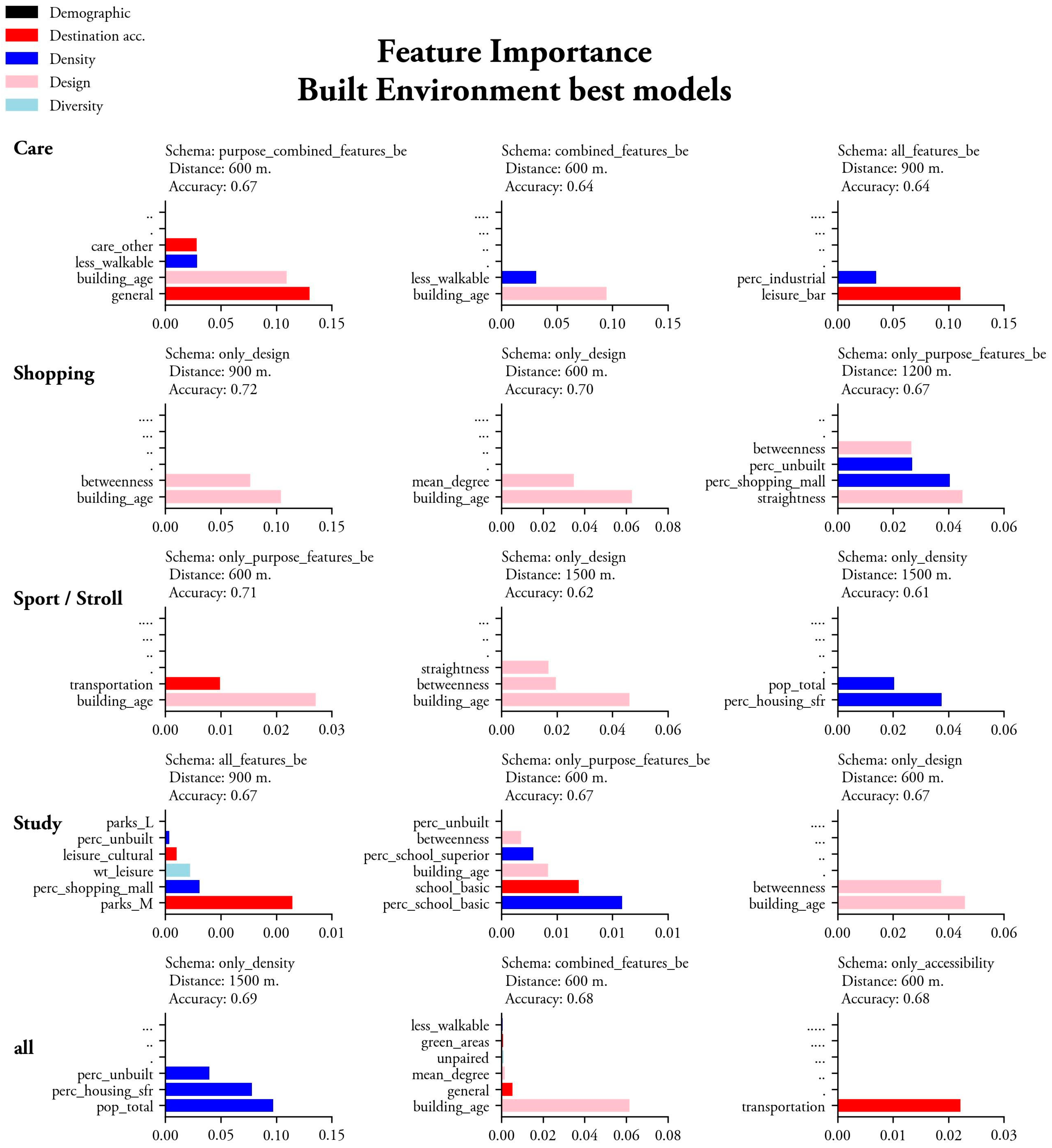
Regarding the schemas used, across all tested configurations, demographic-driven models tended to achieve higher accuracy than those using only built environment factors. When considering only built environment factors, the most accurate models are purpose-driven schemas at 600 m (Shopping and Sport/Stroll trips); and design-focused schemas, especially those incorporating network centrality measures such as betweenness and straightness and density-based schemas, showing competitive accuracy levels.

Confusion matrices provided another (and a bit more disappointing) view of model performance by breaking down the correct and incorrect predictions. In our dataset, all models exhibit high TP, suggesting they effectively differentiate walking trips, but also many models exhibit rather high proportions of FN, showing that some models underestimate nonwalking trips. This behavior suggests that either the selected features are only well suited to predict walking (and in most cases, probably overfitted), but generally show problems in predicting other modes; or that the pooled “other modes” category should be considered in more detail and disaggregation, as it is not as easy to generalize by these models or, in a third stance, that the controls could be actually explaining most of the variation in mode choice.

Table 6. Selected Results.

Distance	Purpose	Schema	Rows	Sample	Accuracy	TN(%)	FN(%)	TP(%)	FP(%)
600	Shopping	only_purpose_features_be	3501	253,705	0.752	12	88	98	2
900	Shopping	only_design	4301	308,649	0.724	16	84	95	5
600	Sport/Stroll	only_purpose_features_be	3331	245,514	0.712	6	94	97	3
600	Shopping	only_design	3501	253,705	0.698	10	90	98	2
1200	All	all_features_dem	21,228	1,560,109	0.694	33	67	87	13
1200	Care	all_features_dem	3571	255,187	0.691	57	43	82	18
1200	Care	all_features_all	3571	255,187	0.691	58	42	77	23
600	All	combined_features_all	13,481	1,001,820	0.689	17	83	95	5
1500	All	only_density	23,560	1,722,129	0.686	37	63	83	17
600	All	combined_features_be	13,481	1,001,820	0.684	16	84	95	5
900	Study	all_features_all	5580	436,009	0.682	30	70	88	12
600	All	only_accessibility	13,481	1,001,820	0.679	13	87	92	8
900	Care	all_features_dem	2964	213,306	0.674	48	52	86	14
900	Study	all_features_be	5580	436,009	0.672	29	71	87	13
1200	Shopping	only_purpose_features_be	4738	338,083	0.671	18	82	91	9
600	Study	only_purpose_features_be	3917	305,460	0.67	19	81	92	8
600	Care	pr_combined_features_be *	2022	145,993	0.669	33	67	85	15
600	Study	only_design	3917	305,460	0.667	18	82	91	9
1500	Sport/Stroll	combined_features_all	5914	420,745	0.656	16	84	94	6
600	Care	combined_features_be	2022	145,993	0.644	32	68	86	14
900	Care	all_features_be	2964	213,306	0.642	44	56	78	22
1200	Leisure	combined_features_all	1095	80,451	0.628	19	81	88	12
1500	Sport/Stroll	only_design	5914	420,745	0.621	14	86	94	6
1500	Sport/Stroll	only_density	5914	420,745	0.605	13	87	93	7

* Abbreviated from purpose_combined_features_be.

shows the selected results, highlighting those models that have at least a TN percentage higher than 30% which, though it is not a great performance, can be seen as a tendency towards a better generalization. When seen from this perspective, it is interesting to note that the best models only keep “All”, “Care”, and “Study” models, which suggests that it is only through larger samples (as in the “All” models) or in these specific purposes where we can detect a relevant influence of factors beyond distance and purpose.

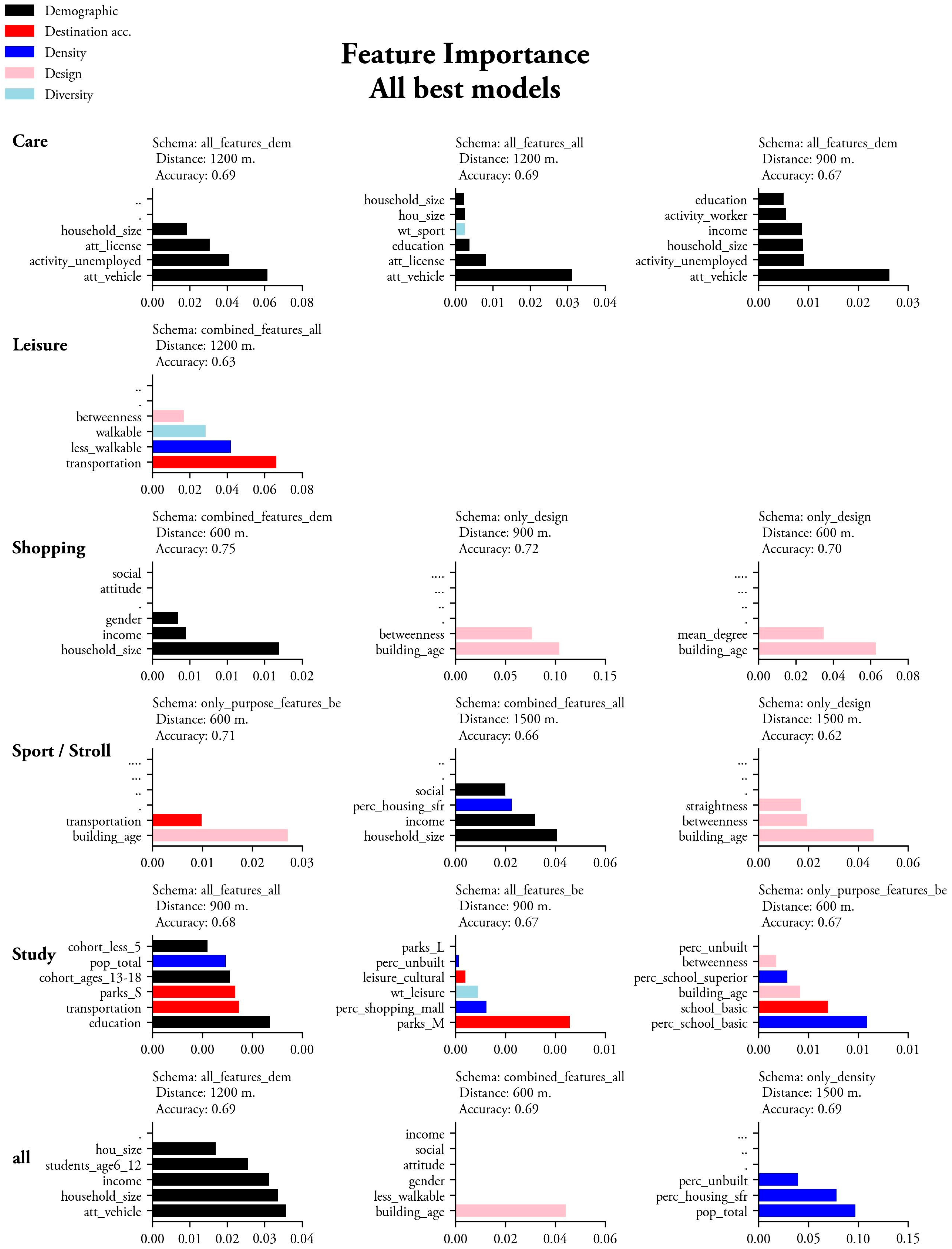
4.2. Permutation Feature Importance

Permutation Feature Importance helped identify the most influential predictors in our models, yet multiple random state iterations only tended to show stable results in models with a better proportion of TN. However, even with the randomness implied by our permutation feature importance approach, features that consistently make it to the final models can be detected in the majority of the iterations performed. Models struggle to generalize our problem, yet still suggest some notable patterns.

As in accuracy patterns, demographics show greater influence on most models. Household size and income were important across models, followed by some age cohorts (younger and older populations) and activity status. Vehicle ownership or driving license were also important in some models. Regarding built environment features, building age consistently ranks as one of the most important across schemas, along with street network characteristics. Other emergent factors are less frequent, such as some accessibility metrics, unbuilt areas, and those associated with urban sprawl, such as single-family residences.

Shopping Trips show interesting patterns. The best model is a combination of Gender, Income, and Household size. The next three models are achieved only by means of built environment features, pointing at design features (they all originated from Only Design schemas) with similar importance. Building Age and features of the “configurational” kind such as centralities seem to be the most important. Also, some less important Density metrics arise, such as “Percentage Unbuilt” or “Percentage Shopping Mall”.

Best models in the “All Purposes” category are similar in accuracy and show expected factor combinations. The best model used Only Demographic schema and pointed at “Has vehicle”, “Household Size”, “Income”, and a more confusing factor of Household Structure (“Students aged 6 to 12”). Another two models kept “Building Age” obliterating all other factors, while the remaining two are first, a combination of characteristic density factors (“Population Density”, “Percentage Unbuilt”, and “Percentage Single Family Residence”) and, second, a model exclusively retaining “Accessibility to Transit”.

Care trips attain the best performance when “Has a vehicle” is present. Also “Has driving license” ranked important in the best three models. Other less informative, yet important features were “Unemployed”, “Household Size”, “Education” or “Income”. These models yielded confusing features in their three best Built Environment-Only models. While the general Combination of Accessibilities and Building Age emerged as very important, other confusing features such as Accessibility to Leisure Bars emerged.

Study models were, once again, more demographic-oriented. However, in this case, the best model also maintains other more informative Built Environment metrics, such as Accessibility to Transit, Small Parks, and Population Density. Level of education and Age Cohorts arise as very important in these models. The best three models only using Built Environment include a very confusing model including Accessibility to Medium Parks, Leisure Diversity, or Percentage of Shopping Mall; another more reasonable model with features capturing Accessibility to different kinds of School Facilities; and another parsimonious model using only Betweenness and Building Age.

Leisure models had a comparatively low accuracy, only managing to obtain one model, composed of Accessibility to Transit, and Density/Diversity of groups of less and more walkable land uses, respectively. Also, Betweenness played a less important role in this purpose. Features in Sport/Stroll trips also yield somewhat confusing models. The best model is a combination of Building Age and Transportation, and the second best is composed mostly of combined Demographic features, such as Household Size and Income, and, notably below in accuracy, models combining either Building Age with Centrality measures (Betweenness and Straightness), and Population Density with Percentage Single-Family Residence, respectively. Figure 1 and Figure 2 show feature importance results.

When considering only those models with TN higher than 30%, we note a slightly more readable set of feature importance results. “All”, “Study” and “Care” models generalize better and still consistently point at demographics and accessibility to relevant facilities, together with features that point to the presence of less walkable environments.

5. Discussion

5.1. Regarding the Distance Threshold Approach

Changes in distance thresholds significantly affect model performance across different purposes. This idea aligns with the high importance and granularity of distance in local mode choice [16,40]. Shorter distances (600–900 m) yielded higher predictive accuracy on average. However, these thresholds reduce the “other modes” class considerably and, after undersampling, models in shorter distances receive a sort of “target leakage” bias that should not be overseen, and can be locally very significant (for instance, in places where other modes are especially less used).

In future works, more sophisticated ways of resampling models, particularly those oversampling minority classes, should be tested, probably taking into account the original modes in the oversampled class. Also, another way of reducing the imbalance class could be focusing directly on those areas where nonwalking behavior in proximity is significant and, while potentially losing data, obtaining more “naturally” balanced samples. The selection of those differentiated areas, however, should be discussed with care.

An implication of distance thresholds is that they constrain the spatial window in which the built environment is measured “around respondents” (in our case, using isochrones). This approach is supported by many reviewed works, from early works such as [21,31], reviews such as [23,24], to more contemporary works such as [87], and the trend of accessibility measurement noted in the 15-Minute City-related work [56,57,58]. We have not considered the sensitivity of metrics to this aggregation approach, as recommended in works like [36,37]. Future steps could include more pedestrian-oriented aggregations such as routes (understanding the role of spatial aggregation in the models), or specifically addressing how model performance varies with distance threshold.

5.2. Regarding Trip Purpose Controls

Purpose controls are a fair approach to user needs, but some categories seem to have bias induced by the lack of further controls such as age, household structure, or income, which are gaining more detailed attention in the literature [30] (for instance, study or care trips have strong age and household implications that were not taken into account). Other models can be biased by limitations of the survey used, such as the Sport/Stroll, the Leisure, and the Care categories, which could also take advantage of further demographic filtering, but also from the selection of destinations considered.

The most accurate models achieved were for shopping purposes and, besides one single model for Sport/Stroll, the second most accurate was in the pooled “All” category. However, only the “All”, “Care” and “Study” models showed some tendency towards a reasonable prediction of nonwalking trips. In some of the categories, quite different feature definitions were achieved, suggesting that similar predictions can be obtained from demographics, built environments, and both kinds of features, yet pointing to demographic features as slightly more important. This could mean that: approaches are interchangeable (could lead to a deeper reflection about the endogeneity of travel and residential location seen in [25,67], or they have similar importance when making choice predictions (with a slightly more relevant role of demographics), being consistent with ideas expressed in [23,24,27].

5.3. Regarding the Schemas and Features Used in the Models

Models using built environment schemas exhibit higher FN rates compared to those incorporating demographics, reinforcing the idea that the built environment alone does not fully explain mode choice decisions. Schemas having demographic definitions were the most accurate, followed by purpose-driven, and those design-centered. In general, schemas using more disaggregated variables (such as those using all variables), ended up having some extraneous predictors, maybe due to the inflexible feature selection. In this sense, future steps could involve relaxing the correlation threshold (or specifically inspecting how the models’ performance varies with this parameter), allowing experts entering the loop of feature selection (manually validating the elimination of features, or simply focusing on one particular “D” at a time), or using more sophisticated grouping techniques, helping to maintain relevance, while avoiding multicollinearity.

In models including demographics in their final feature sets, the most important predictors align with established findings in proximity research: household size and income are strong determinants [38,42,43]. Some age cohorts and activity status emerged in the final models -particularly younger and older populations-, consistent with their importance in recent research [30]. Features such as vehicle ownership or driving license were very important in some models, pointing at the dilemma of endogeneity and residential self-selection described in the literature [25,67]. These features, however, can be very informative as a target variable, or controlled for in future works. In general, it can be said that features revolving around ideas from activity travel research, and theories like habit formation, have a relevant role in studying proximity behavior [59,62].

Regarding the Built Environment factors, Building Age and network centrality such as Degree, Straightness, or Betweenness emerged in many models strongly biased towards walking trips. This result is interesting and has a double reading: On one hand, these features “mask” many other predictors of the built environment, which could be consistent with findings of configurational theories such as Space Syntax or Complex Networks [48]. On the other hand, the interplay between configuration and period might be pointing to a more complex condition of metropolitan structure that could be a proxy for walkability, and it is comparable to the results in [91]. In this sense, though the results are consistent, it remains a future task to inspect further nuances of both regional and local configurational arrangements and, we acknowledge, if this is a particular condition of the MRM (which exhibits many areas or historical urban fabric which, in most cases, are centers that exhibit prominence of walking trips). As expressed in [21], the importance is not on the factor itself (in our case, configuration or regional arrangement), but what it brings along with it. Thus, features like Building Age should be further reviewed for disaggregation into “smaller” design components.

Accessibility, Density, and Diversity metrics yielded more confusing results. Combinations of Accessibilities and Accessibility to Transit were important in some highly accurate models (particularly in those generalizing the problem better), but in other models (and probably highly correlated to some alternative and more informative metric) confusing features emerged, with little or no reasonable connection to the modeled purpose. Regarding density, some accurate models were obtained which pointed to factors preventing walkability, such as combinations of Percentage Single-Family Residence or Percentage Undeveloped Land. In our case, it is disappointing that other more elaborate indices such as the Walkable Trips capturing Diversity through complementarity did not make it almost into any models, when a good generalization was not achieved.

A less “unsupervised” feature selection process, and a more nuanced study through previous control, could help to unveil these factors’ implications in walking behavior. In this sense, a more targeted or conscious use of conditions of accessibility or density could be carried out. For instance, they could be used for filtering urban configurations with no pedestrian accessibility before modeling, differentiating more complex “neighborhood types” such as urban sprawl or other classes of residential neighborhoods, through these factors, as in early approaches such as [21,33], or improving “compliance metrics” such as [51], prior to predictive modeling. Also, introducing all these different “D’s” in single models could simply lead to the confusion expressed in [26], and a simplification of the approach (for instance, only using complex indices of accessibility that account for density and diversity) could improve the readability of results.

5.4. Regarding Informational Power

Policy-wise, these results are still rather limited. In general, better accuracy with less overfitting could be useful for agnostic simulation strategies in which the target is to obtain accurate pedestrian flow prediction. However, not being able to generalize the importance of the associated factors (and, particularly, those that can be influenced “by policy design”), hinders the ability of potential simulation efforts in terms of scenario building. Results are also lacking spatial information, which obscures a critical need not only for knowing “what to do” but also “where to intervene” in planning practice. This issue could be addressed by using alternative feature importance strategies such as SHAP values, which yield individual metrics for observations, that could potentially be located and studied in terms of spatial patterns. Regarding spatial patterns, another interesting idea could be to spatially cluster (for instance, using unsupervised ML workflows such as DBScan, or Local Indicators of Spatial Autocorrelation) those features that seem relevant across models, and perform more controlled comparisons. In any case, helping planners or local experts in the discussion on the effects of the social and built environment on proximity is an appealing future step.

The ability of RF models to converge in many different data scenarios is interesting for a global exploration of these datasets. In the reviewed works on the study of urban proximity, a call for accounting for “arrays” of distances, abilities, or needs across users is encouraged, and other statistical approaches, such as linear or logit models (derived from translations of utility theory, among others), would involve a more costly process of individual model fitting. However, when it comes to comparison across models, the proposed methodology yields incomparable results (feature importance cannot be compared across different models). In this sense, a more controlled feature selection could be helpful for a further iteration in which, after a robust selection, the complete matrix of models could be fit with more “readable” models of the linear or logit kind, yielding readable metrics such as elasticities, more readable model errors, or allowing for the study of “unexplained” variation through intercepts, latent variables, or random utility models.

Finally, some critical questions on endogeneity, such as the residential self-selection or the local vs regional accessibility questions, were not addressed by this method. The former, however, could be addressed by using some of the discarded “attitudinal” variables in the EDM2018 (which held answers such as “I rather walk” or “I rather drive”, which could be further targeted instead of mode choice, to then inspect the similarities and differences. The case of regional vs local accessibility could be further explored by using information about “competing” modes, such as daily distances covered by car from a particular TAZ, which could help explain certain local mode choice behavior, linking, for instance, daily local trips with daily longer commute (such as intermediate “drop-offs” or errands run on the way to work.

6. Conclusions

This study performed a complete feature selection workflow on a very diverse set of predictors, attempting to understand if general regularities emerge from their association with walking behavior. Results ended up yielding mixed suggestions in terms of heuristic power to study urban proximity. In a broad sense, ML approaches seem to struggle with generalizing the problem of local travel mode choice, biasing results towards pedestrian travel, and only achieving balanced results in either large samples or in Care and Study models. However, approaching feature selection only with performance in mind, results in a loss of explanatory power, as the factors (and their importance) yielded by models still need further expert interpretation to possibly inform policy.

Some positive findings were made. Many models reveal a high -although rather biased- predictive power using little information on street configurations and broad building periods, which is an advantage for models that only need to simulate this local behavior, or studies which focus on particular configurations of the urban form revealed by clustering or other kinds of spatial analysis, which could help to reveal “states of proximity” in which walking behavior could need to be modeled differently. Also, models only using demographic variables can be an interesting approach, as this information is broadly available, helping to address endogeneity problems such as the “residential self-selection problem”.

Overall, an exploration like the one presented here yielded an interesting set of predictors across all models, which could be further refined and used in more domain-driven models such as Logit or Probit models, or less explicable Machine Learning models (which are commonly more accurate). Future research should explore hybrid modeling approaches combining econometric and machine learning techniques to enhance both interpretability and predictive power. If some of the ambiguities found in this work are sorted out, ML models could not only detect important features, but also discriminate between those that have linear or non-linear relationships with choice, or those that are “better together”, further improving the specification of Linear or Logit models which, to our view, seems to be the more informative approach still.

The downsides were that too many models ended up having a disappointing behavior in predicting other modes; being formed by features which become misleading or counterintuitive; some attitudinal and sociodemographic predictors seem to point out social patterns which are not directly interpretable (or endogenous to travel mode choice), and need further research. The first issue could be mitigated by the further implementation of variable selection which takes into account domain-driven recommendations. The second could use a prior investigation of social patterns in the targeted geography, and could be adjusted to apply further control to experiments on local mode choice.

The issue with the poor classification of other modes could be addressed by adding new mode alternatives to the models, and addressing sample balance in a more sophisticated “mode-conscious” way. Also, extremely short threshold distances might diminish samples very much, to a point in which comparing walking and other modes becomes trivial, so distance should be kept at the maximum ranges of observed walking trips (in our case, the 1500 m threshold), in order to fully be able to compare modes when seeking to inform “modal shifts”.

Policy implications need to be taken with care, in view of the results. While models have been proven very sensitive to the effects of proximity thresholds and purpose, the sets of factors suggested are sometimes misleading, and models struggle to generalize the choice to walk against other modes. Some of the less biased modes point to urban configuration proxies, demographic features, and known characteristics of less walkable environments. Also, Care and Study show the best overall performances, suggesting that these activities and the most implied population segments seem an interesting vector to further inspect the combined effects of the social and built environment as a tool for policy information.