Abstract
Smart city initiatives highlight the vital role of Intelligent Transportation Systems (ITS), which remain underexplored with limited AI-driven solutions integration in real-time urban traffic management across African cities. ITS is crucial to enhance urban mobility efficiency and sustainability to address growing mobility challenges in the era of swift African urbanization. This paper proposes an AI-driven predictive model for the Travel Time Index (TTI), a key metric quantifying urban traffic congestion and mobility performance. Using spatio-temporal analysis, neural networks, and advanced machine learning algorithms, the model processes real-time, multimodal traffic data, capturing congestion patterns, TTI fluctuations, and complex urban travel dynamics, focusing on Casablanca, Morocco, as a smart city case study. Five predictive modeling approaches were carefully selected and rigorously evaluated: Multivariate Linear Regression (MLR), Random Forest (RF), Gradient Boosting, Multilayer Perceptron (MLP), and Support Vector Regression (SVR). Their performance was assessed using standard evaluation metrics: Mean Absolute Error (MAE), Mean Squared Error (MSE), Root Mean Squared Error (RMSE), and R-squared (R2). All models achieved high accuracy, with Random Forest ranking highest (MAE = 0.315, R2 = 0.985). Beyond prediction, the methodology incorporates feature importance analysis and hyperparameter tuning via GridSearchCV to improve operational performance and practical applicability across evolving traffic ecosystems. Hyperparameter optimization further enhanced Random Forest’s accuracy (MAE = 0.220, R2 = 0.988). The findings demonstrate improved travel time estimation and congestion management capabilities, offering a scalable, adaptable framework to guide data-driven mobility strategies in diverse urban settings and provide actionable insights for urban planners, policymakers, and mobility stakeholders.
1. Introduction
Urbanization is a defining global phenomenon shaping the 21st century, with profound implications for urban mobility and infrastructure planning. As of 2025, approximately 58% of the world’s population resides in urban areas, a figure projected to rise to nearly 70% by 2050 according to United Nations estimates [1].
This rapid urban growth is particularly pronounced in Asia and Africa, where urban populations are expanding at unprecedented rates, as shown in the United Nations report of urban population by continent (1950 and 2024 comparison) [2]. According to the data in this report, urbanization levels were considerably low in 1950, especially in these continents, and only around 14% of the African population lived in urban areas. Conversely, by 2024, these regions have undergone significant urban expansion driven by economic development, industrialization, and improved living conditions [3].
Africa’s urbanization rate, currently reaching approximately 45%, is expected to accelerate significantly in the coming decades, driven by demographic shifts and rural-to-urban migration [4]. Morocco exemplifies this trend in the African context, with its urban population increasing steadily, as stated in the latest report released in December 2024 by the Higher Planning Commission (HCP), an independent government statistical institution in Morocco. Recent data published indicate that over 62% of Moroccans now live in urban settlements, reflecting ongoing migration and urban expansion. It also reveals the evolution of the urban population and urbanization rate from 1994 to 2024 (%), highlighting that the urbanization of the Moroccan population has increased from 51.4% in 1994 to 62.8% in 2024 [5,6]. In Morocco, the urbanization process has been accompanied by significant infrastructure development, including the expansion of the highway network from 850 km in 2008 to 1400 km in 2015. While this has facilitated increased vehicular mobility, it has also introduced challenges such as traffic congestion, longer travel times, and environmental pollution, particularly in major cities like Casablanca [7].
The Travel Time Index (TTI), a key metric measuring congestion and delays, often reveals substantial variability that traditional traffic management systems, reliant on static policies and historical data, struggle to manage and predict, and accurately [8]. Conventional statistical methods, such as Historical Averages (HA) and Auto-Regressive Integrated Moving Average (ARIMA) models, have been used for traffic forecasting but are limited in capturing the nonlinear, dynamic, and context-dependent nature of urban traffic flows [9]. These existing traffic management systems have been pointed out [10,11,12,13]. Recent research in this field emphasizes the need for adaptive solutions not only to cope with evolving traffic patterns in smart cities [14], but also to manage and alleviate congestion issues as they arise [3,10,15,16,17]. The emergence of smart city initiatives has catalyzed the integration of Intelligent Transportation Systems (ITS) that leverage real-time data and Artificial Intelligence (AI) to enhance urban mobility [18,19,20,21]. Machine Learning (ML) and Deep Learning (DL) models, including Random Forest, XGBoost, Long Short-Term Memory (LSTM), Graph Neural Network (GNN), and Convolutional Neural Networks (CNN), have demonstrated potential to improve traffic prediction accuracy by capturing complex temporal and spatial traffic patterns [22,23,24,25,26].
For example, Ref. [27] showed that ensemble methods like Random Forest and Gradient Boosting (XGBoost) outperform traditional statistical models in predicting short-term traffic volume, achieving lower prediction errors and better generalization. Similarly, Ref. [28] used Google Maps data to train ML models for congestion prediction, highlighting the importance of integrating real-time data sources for improved accuracy. Ref. [29] conducted a comparative study showing that DL models like Recurrent Neural Networks (RNNs) effectively capture temporal dependencies and periodicity in traffic data, enabling accurate forecasts [30]. To further highlight the vital role of smart transportation systems in travel time prediction, especially during extreme events and natural disasters, this recent study proposes a GNN-based framework for estimating shortest travel distances and recommending routes, particularly during floods, enhancing emergency planning by efficiently calculating evacuation routes and minimizing response times in coastal urban areas [31].
In the Moroccan context, Ref. [32] examined the challenges of predicting traffic volumes using historical data. The study revealed that daily traffic volume data often contained anomalies due to external factors, including national events, which caused irregular spikes and dips in traffic. To address these inconsistencies, a robust data filtering approach was adopted, using techniques such as moving averages and Seasonal adjustment to smooth out noise and improve the reliability of the forecasted data. This emphasized the importance of data preprocessing and validation in traffic studies, demonstrating that well-executed analysis can effectively inform infrastructure planning and resource allocation [33]. Despite advancements in traffic prediction, current research often focuses on isolated AI models or historical datasets, with limited integration of real-time multimodal transport data such as private vehicle flows, public transit usage, and network connectivity metrics [34,35]. This exhibits limitations in flexibility and responsiveness to real-time traffic variations [36].
Furthermore, there is a scarcity of comparative studies evaluating multiple AI algorithms for TTI forecasting, particularly in the African and Moroccan urban contexts [8]. While global research on AI-based traffic prediction is extensive, there is a notable lack of studies evaluating multiple AI algorithms specifically for TTI forecasting in African cities such as Casablanca, where urbanization and traffic patterns differ significantly from developed countries. Moreover, it is essential to mention that several challenges persist due to data quality and anomaly handling [12,37,38]. Urban traffic data often contains anomalies due to events, sensor errors, or irregular traffic patterns. Robust preprocessing techniques are necessary to improve data reliability, as highlighted in studies of Moroccan highway traffic volume forecasting [32]. Another notable gap in the literature is regarding the integration of hyperparameter tuning methods to optimize model performance in real-world smart city environments, which is often overlooked [39]. This paper aims to fill these gaps by developing comprehensive AI-predictive models with accuracy and enhanced precision for dynamic adaptation to evolving traffic conditions. The main contribution of this research is a new integrated implementation of real-time traffic data sourced from the Waze API, and various ML and DL algorithms to predict the Travel Time Index, and its accuracy enhancement through hyperparameter optimization. These significant improvements remain very promising for smart city applications. This research contributes to the growing body of knowledge on AI-powered urban mobility solutions for African cities, focusing on the Moroccan context and the challenges faced by cities like Casablanca. It advances the state of the art by bridging the gap between theoretical AI models and real-world traffic data, providing policymakers and urban planners with valuable insights for alleviating congestion and promoting sustainable urban mobility.
2. Study Area: Casablanca Smart City Context
Casablanca, Morocco’s largest and most densely populated city, is the principal city of the Casablanca-Settat region, covering 19,448 km2 with 7,689,000 inhabitants Figure 1. The HCP’s General Population and Housing Census (RGPH) of 2024 shows an estimated population of 3,662,436, with 3.236 million residents in 2025 [6]. This growth is consistent with long-term trends, as the population expanded from 625,435 in 1950 to over 4 million today [6]. The city’s transportation infrastructure is diverse and multimodal, with a 23 km urban expressway and a 34 km motorway that integrates Casablanca into the national highway network. However, the city faces escalating congestion challenges due to a dramatic increase in registered vehicles.
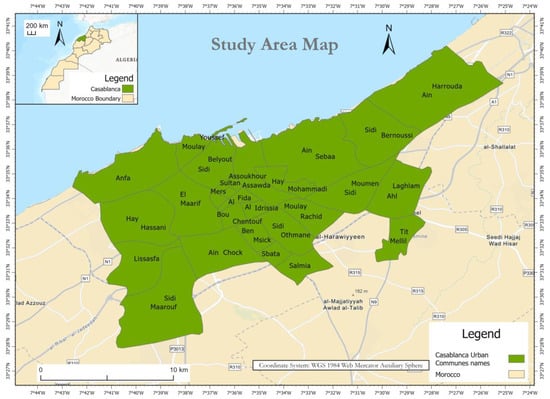
Figure 1.
Research Study Area.
The latest report of MobiliseYourCity Global Monitor 2025 where the city of Casablanca is a partner city within the Project of management assistance to the Sustainable Urban Mobility Plan (SUMP), showed that formal public transport is accounting for about 13%, Informal public transport act for 6%, Walking represents 60%, Private cars about 13%, Private motorbikes or 2-wheelers are only 4%, and Taxis represent 4% [40].
The urban morphology of Casablanca reveals a declining city center population alongside rapid growth in satellite municipalities, driven by housing affordability and changing socio-economic dynamics. This spatial redistribution has altered travel behavior, increasing reliance on private vehicles and necessitating integrated multimodal transport solutions. In summary, Casablanca’s high population density, diverse transport modes, expanding infrastructure, socio-economic dynamics, and significant need for AI-Driven mobility research justify its selection as the study area.
3. Data, Materials, and Methodology
In this section, we introduce the model description for the AI-powered predictive framework for Travel Time Index (TTI). Firstly, we present the study area and the motivations behind the chosen city with the structure of the proposed model, which integrates urban mobility data, machine learning, and deep learning algorithms, alongside the performance indicators. This includes the spatiotemporal data processing pipeline and the implementation steps for model development. Then, we describe the details of the predictive selected models and the hyperparameter tuning application, a process that encompasses optimizing model parameters. Eventually, we highlight the comparative evaluation of our developed models in prediction tasks. Conceptually, our developed model predicts the Travel Time Index (TTI) based on real-time data acquired from the Waze, the navigation mobile application, by incorporating geospatial data, time-dependent variables, and other auxiliary attributes. Waze, by definition, is a mapping and navigation app powered by a crowd-sourced community [41]. It uses user-generated data to provide real-time traffic information, including details of accidents, roadworks, and other potential hazards. To start, we implemented our first model, Multivariate Linear Regression (MLR), considered as a fundamental statistical technique for modeling the linear relationship between multiple independent variables(predictors) and a single dependent variable (the traffic metric we want to predict, which is the TTI). Due to its simplicity and interpretability, it is a common baseline.
The existing literature commonly highlights its assumptions, such as linearity, independent errors, and constant variance [42]. While MLR is effective for linear relationships, it has difficulty capturing complex, nonlinear patterns in data, as discussed in modern overviews such as [43]. Then, we identified patterns of congestion during different hours of the day. After that, we trained other models to predict TTI, and we have chosen: Random Forest Regressor, a highly suitable model for traffic and congestion prediction due to its ability to capture complex, non-linear relationships and interactions between various traffic factors. Ref. [44], a landmark paper, introduced this powerful algorithm. Studies often mention its ability to handle high-dimensional data and its resistance to overfitting, as illustrated in early applications from [45,46,47,48] advanced the understanding of its functioning, they specifically addressed feature importance.
Gradient Boosting (XGBoost) is considered a powerful model for structured data, and is particularly well-suited for predicting traffic and congestion, and it often achieves better results than other methods. A significant corpus of literature has demonstrated the predictive accuracy and processing speed of XGBoost, as detailed in its key paper by [49]. The model has been proven effective in the management of non-linearities and complex interactions; however, it is susceptible to overfitting if not duly tuned, a notion that has been thoroughly explicated in tutorials by [50].
Neural Networks or Multi-Layer Perceptrons (MLP Regressor) consist of interconnected layers of nodes (neurons) with activation functions. Multilayer perceptron (MLP) regressors possess the capacity to process highly complex, non-linear patterns, particularly in the context of large and complex traffic databases. The literature highlights their modeling capacity of complex patterns, with foundational concepts based on backpropagation [51]. Overviews of deep learning, including MLPs and their applications, are available in publications authored by [52], as well as other sources such as the textbook by [53]. Lastly, we used Support Vector Regression (SVR). This algorithm is a Support Vector Machine (SVM). SVR identifies a hyperplane that best fits the data within a specified margin of tolerance extension for regression tasks. Effectively, it handles nonlinear relationships with kernel functions. SVR’s theoretical basis is detailed in [54], and early practical formulations were presented by [55,56] wrote a widely cited tutorial on SVR’s prediction tasking, and [57] covered it in a larger context of machine learning. All selected algorithms perform regression, meaning they predict continuous outputs based on input features. Regressor models in machine and deep learning are specifically designed for prediction tasks where the output is continuous, not categorical. In other words, regression models are the right tool for estimating numeric outcomes, such as TTI in minutes. These algorithms were implemented using Python libraries. Pandas was used for data manipulation. NumPy was used for numerical computations. Matplotlib (3.10.0) and Seaborn (0.13.2) for generating plots, charts, and histograms. GeoPandas for geographic data manipulation and finally, Scikit-Learn were used for machine learning features.
3.1. Data Sources, Collection, and Preprocessing
This section outlines the data sources used and the methodology adopted for building and evaluating the predictive model for Travel Time Index (TTI) within the urban context of Casablanca. A hybrid data-driven approach is employed, combining real-time traffic information, geospatial data through geocoding tools to support the development of robust AI-based predicting models. In this study, we employed the Waze dataset to analyze traffic congestion patterns across the city of Casablanca [58,59]. Waze, a community-based navigation application, serves as a valuable source of real-time traffic data collected via GPS-enabled mobile devices from millions of active users called “Wazers”. The dataset used in this research was obtained through the Waze Application Programming Interface (API), which provides comprehensive probe data including real-time travel updates, congestion alerts, incident reports, and geolocation metadata. Specifically, the Waze API Calculator provides two distinct time-based metrics for each trajectory: real and free-flow travel time. The real travel time measures how long vehicles take to traverse a road segment in traffic, and free-flow time shows the typical time in the absence of traffic congestion. These complementary metrics allowed for a nuanced understanding of traffic behavior and performance variability across different zones of the city.
To construct the dataset, travel time and distance data across 20 randomly selected trajectories within each of the 26 selected municipalities of Casablanca city were collected [58]. This dataset was retrieved hourly over the course of one full week, from Monday through Sunday, enabling the observation of both peak and off-peak travel patterns. This week-long dataset balances temporal representativeness while avoiding performance issues from long-term urban changes during extended periods.
For each trajectory, the Waze Calculator provided detailed information on Vehicular (i.e., motorized) travel time at each hour and route distance between origin and destination. Using this information, the Travel Time Index at each hour and per trajectory was calculated within each zone.
Table 1 presents the attributes of the 26 selected Casablanca urban communes.

Table 1.
Attributes Table of Casablanca Urban Communes.
The data collection process was repeated continuously, 24 h a day, over seven days, resulting in a highly granular temporal dataset. In total, the trajectories were queried 168 times each (24 h × 7 days), across 440 unique routes. The data-cleaning and preprocessing of the traffic dataset proceeded as follows: Initially, all non-essential metadata and irrelevant columns returned by the Waze API were excluded, and the remaining columns were properly renamed to facilitate downstream processing. Next, numerical columns such as travel times, distances, and Travel Time Index (TTI) were converted to numeric formats using Pandas open-source Python library, and duplicate column names were uniquely renamed. Then, missing values due to incomplete data from mobile devices or API issues were eliminated by dropping completely NaN columns and resetting proper indexing. Additionally, duplicate records caused by multiple Waze users reporting the same road segment at the same minute are identified and removed to avoid bias. After that, the Interquartile Range Method (IQR) was used to remove detected outliers in each hourly column. These anomalies’ detection helps to keep data consistent while preserving meaningful traffic fluctuation signals. Finally, the cleaned and processed dataset was organized into a Pandas DataFrame structure, with each row representing an origin-destination pair and hourly TTI values listed in the columns. This structure provides a clear input feature set for training and evaluating our models. These systematic preprocessing steps ensure high data quality and that Waze traffic dataset accurately reflects urban mobility conditions in Casablanca city.
After rigorous cleaning, encoding, and formatting, the final dataset yielded 73,920 individual records of travel times and distances entries and 13 descriptive attributes such as postal code for each commune, Coordinates (Latitude and Longitude) for both the origin and destination, distance, Real Time Travel (RTT), and the calculated Travel Time Index (TTI). The processed dataset was structured into a comprehensive CSV file format, where each of the 26 communes was represented as a row. This dataset integrates both real-time traffic dynamics, providing a solid foundation for the analysis and prediction of urban mobility trends in Casablanca city.
3.2. Research Methodology
The aim of our study is twofold: first, to analyze spatio-temporal variations, and second, to predict traffic congestion spots within the urban municipalities of Casablanca. In order to achieve this objective, we initially considered the Travel Time Index (TTI) as a potential indicator of congestion level. The TTI is calculated based on real-time traffic data acquired from the Waze API. Then, we statistically analyzed the variance of the TTI over the time series selected. Afterwards, we built a predictive model based on various machine learning and deep learning algorithms to predict the TTI as a target variable. Finally, we trained and tested our model to evaluate and compare the accuracy of each model using specific evaluation metrics. The following Figure 2 illustrates the proposed data collection and the several key steps involved in the prediction process.
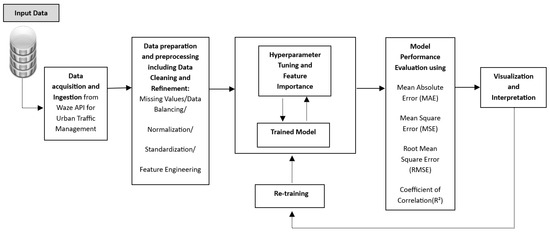
Figure 2.
AI Predictive Model Pipelines: Streamlining the Model Development Process.
3.3. Model Building
Building upon the insights obtained from the analysis, we then proceeded to the predictive modeling phase, and we developed an AI model to predict the Travel Time Index (TTI). We started with the Linear Regression (LR) model [43], then compared with Random Forest (RF) [48], Gradient Boosting (XGBoost) [49], Multi-Layer Perceptron of Neural Networks (MLP) [52], and Support Vector Regression (SVR) [56].
In this segment of our research, we developed and compared several machine learning alongside with neural network models to predict the Travel Time Index (TTI), which represents the ratio of travel time in peak conditions to free-flow conditions. Put another way, the Travel Time Index represents the average additional time required to travel during peak hours compared to traveling during off hours [60]. The Travel Time Index (TTI) presents several advantages, notably its interpretability, ease of estimation, and its ability to effectively capture traffic congestion in terms of both temporal delay and spatial extent. This metric, introduced by the Texas A&M Transportation Institute in the early 2000s, has since become a widely adopted measure for quantifying urban traffic congestion following Equation (1) [61]:
where
- is the average travel time during congested periods,
- is the travel time under ideal (uncongested) conditions.
The modeling task aims to forecast TTI for the next hour using historical hourly TTI values as features. To begin, we selected all time-based columns (0, 1, 2, …, 23) from the cleaned dataset corresponding to Mondays. These columns represent hourly TTI values across the day. We used all available columns except the last one as input features (x) and designated the final column, which corresponds to the TTI at the subsequent hour as the target variable (y). The predictive function is defined as Equation (2):
where
- y is the target/dependent variable (TTI)
- is the intercept (bias term)
- are the slopes (weights)
- are the features (independent variables)
- the error
To support modeling and validation, the data was split into 80% for training and 20% for testing. The training function uses the training subset to fit each of the five selected models by learning patterns and relationships in the data. The test function then evaluates each model’s performance using the test subset, providing an allocated dataset score that measures predictive accuracy on unseen data. This approach ensures robust assessment of each model’s generalization capability.
The evaluation was based on the following performance metrics:
- Mean Absolute Error (MAE) measures the average magnitude of the errors between predicted values and actual observations, without considering their direction as defined in Equation (3) [62]. It provides an intuitive indication of how far predictions deviate from true values on average. Because it uses absolute values, MAE treats all errors equally and is less sensitive to outliers.
- n is the number of observations,
- is the observed (actual) value,
- is the predicted value.
MAE’s lower value is desirable because it indicates that the actual value and prediction are close to each other.
- Mean Squared Error (MSE) calculates the average of the squared differences between predicted and actual values. By squaring the errors, it penalizes larger errors more heavily, making it sensitive to outliers. MSE is commonly used to assess overall model accuracy and is especially useful during model training. The mathematical expression is given below (Equation (4)):
where the variables are as defined above.
- Root Mean Squared Error (RMSE) is the square root of the Mean Squared Error. It expresses the average magnitude of prediction errors in the original units of the target variable as defined in Equation (5). RMSE emphasizes larger errors due to the squaring step and is widely used to evaluate regression model performance [63,64].
- Coefficient of Determination (R2 Score) measures the proportion of variance in the observed data that is explained by the model [65] in Equation (6). It ranges from 0 to 1, where values closer to 1 indicate that the model explains most of the variability in the target variable, reflecting strong predictive power.
A dedicated function was used to streamline the training and evaluation process: Each model’s performance metrics were stored and subsequently compiled into a ‘DataFrame’ for comparison. The resulting ‘DataFrame’ summarizes the accuracy and generalization capability of each model. This comparison provides a basis for selecting the most appropriate predictive model for real-time or near-real-time estimation of TTI.
4. Results Analysis and Discussions
4.1. Statistical Analysis
We analyze the distribution of TTI values across different hours using histograms and box plots. The box plot provided in Figure 3 effectively visualizes the hourly distribution of Travel Time Index (TTI) values, revealing distinct congestion patterns. The median TTI, shown as the horizontal line in the box (50th percentile), represents the central congestion level (the central value of TTI during that hour) and generally increases from the early morning hours (around 2 a.m.) to a peak in the late afternoon/early evening (approximately 5:00–7:00 p.m.), indicating typical rush hour behavior. The interquartile range (IQR = Q3 − Q1), represented by the height of the boxes, indicates variability. Taller boxes, especially during peak hours, suggest a wider spread of congestion levels and more inconsistent traffic conditions. On the other hand, shorter boxes suggest more stable traffic. Plotted as individual points, outliers appear more frequently during afternoon and evening peaks, signifying occasional severe congestion events likely attributable to incidents or extreme conditions. The overall shape of the boxes and whiskers suggests positive skewness in many hours. The median is often closer to the lower quartile, and the upper whiskers are longer. This indicates that while typical congestion might be moderate, there are occasional instances of significantly higher congestion.
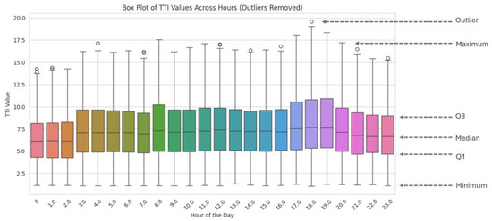
Figure 3.
Box Plot of TTI Values Across Hours.
As part of the statistical analysis of the collected data, and to elucidate the temporal dynamics of traffic congestion, we presented in Figure 4 a correlation matrix heatmap visualizing the pairs correlations between Traffic Travel Index (TTI) values across distinct hours of the day, ranging from 00:00 to 23:00. Both the row and column axes represent this same hourly sequence, enabling a comprehensive examination of how TTI at any given hour relates to TTI at all other hours. Strong positive correlations, indicated by deep red cells, signify a gradual buildup and subsequent dissipation of congestion, where TTI values tend to move in alignment across consecutive hours. Conversely, weak correlations, depicted by cells close to white or with minimal color intensity, suggest periods of unpredictable traffic behavior where conditions at one hour have little bearing on another. Inverse relationships, represented by blue cells, highlight instances where high congestion at an earlier hour might correspond to lower congestion at a later hour, potentially due to traffic redistribution or the resolution of an initial disruption. This visualization serves to quantitatively assess the temporal dependency structure of traffic congestion patterns.
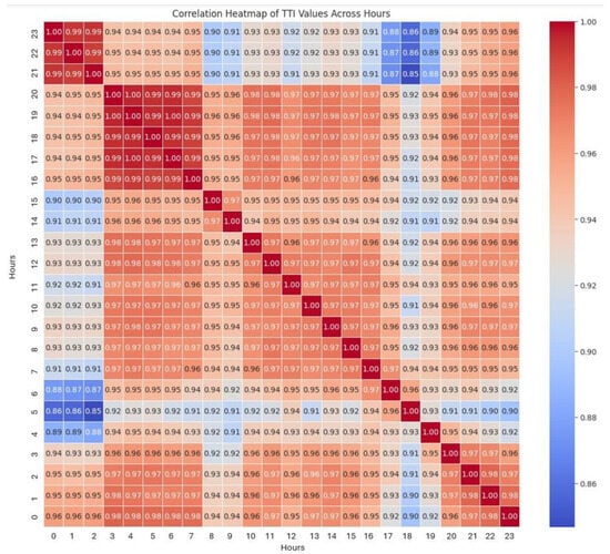
Figure 4.
Correlation matrix Heatmap of the TTI values for different hours.
4.2. Time Series Analysis
This section of our experiment tests the hypothesis that the traffic patterns of the city of Casablanca are evolving significantly over the weekdays and weekends. To evidence that, we undertook a comprehensive analysis of how TTI evolves throughout various times of the day to meticulously identify and effectively assess peak congestion hours during different periods, allowing us to draw meaningful insights into traffic patterns.
As depicted in Figure 5, the TTI time series illustrates predictable urban traffic cycles, with the most severe congestion occurring during the evening peak (from 17:00 to 19:00). A secondary, more moderate plateau is observed midday (from 11:00 to 15:00), while overnight hours (from 00:00 to 06:00) maintain minimal traffic interference. The raw line preserves hourly granularity, exposing natural fluctuations and potential anomalies, whereas the smoothed curve emphasizes macro-level patterns without the noise. Presenting both allows for precise inspection and high-level trend recognition simultaneously, critical for robust traffic modeling or anomaly detection.
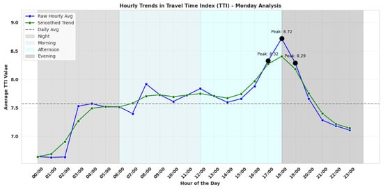
Figure 5.
Hourly Trends in Travel Time Index for one day Sample Analysis.
4.3. Geospatial Analysis
This part of the analysis is dedicated to the extraction of detailed coordinates and the visualization of various traffic trajectories to detect spatial congestion patterns. These patterns are critical for understanding and mitigating traffic issues.
Accordingly, we used K-means clustering algorithms to identify traffic hotspots in Casablanca, as illustrated in Figure 6.
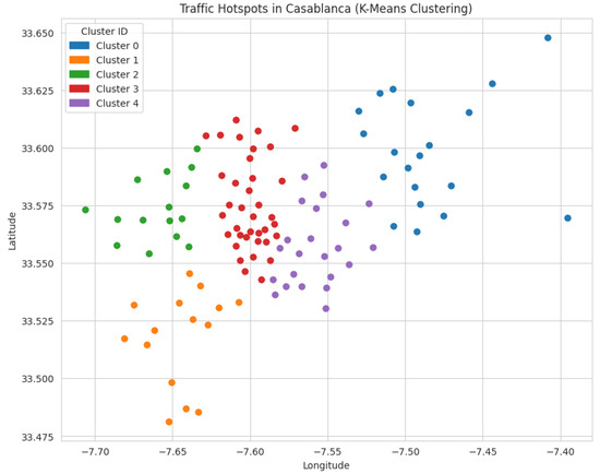
Figure 6.
Traffic Hotspots in Casablanca (K-Means Clustering).
The resulting plot, as illustrated in Figure 6, shows the distribution of data points across the identified clusters, revealing five distinct major congestion hotspots. These hotspots represent high-traffic junctions and main roads in Casablanca.
As shown in Figure 7, the spatial distribution of urban traffic congestion across Casablanca is visualized using the Travel Time Index (TTI) as a congestion level indicator. The map was generated through Geographic Information System (GIS)-based spatial analysis using Inverse Distance Weighted (IDW) as a deterministic method for spatial interpolation, with TTI values calculated for selected communes based on travel time delays during peak hours compared to free-flow conditions. Areas with dense TTI values, depicted in warm red color, indicate more severe congestion levels, particularly in central and economically active zones such as Maarif, Sidi Belyout, and Al Fida. Figure 7 highlights the critical congestion raster and provides a foundational spatial layer for model training and evaluation. This reinforces the importance of localized, data-driven strategies to enhance urban mobility planning in the context of smart and resilient African cities [66,67].
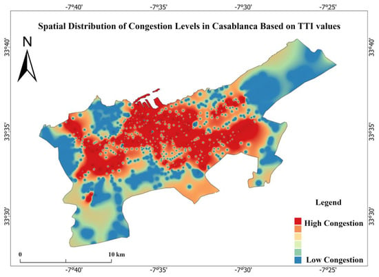
Figure 7.
Spatial Distribution of Urban Congestion Levels in Casablanca Based on TTI Value Range. Coordinate System: WGS 1984 Web Mercator Auxiliary Sphere.
In summary, the data analysis conducted in this section highlights traffic patterns, peak congestion hours, and spatial congestion areas, thereby offering a solid foundation for the subsequent model building presented in the next section.
4.4. Predictive Model Performance Evaluation
The following Figure 8 summarizes the performance of the evaluated models in predicting the Travel Time Index (TTI), based on four key metrics: Mean Absolute Error (MAE), Mean Squared Error (MSE), Root Mean Squared Error (RMSE), and R-squared (R2). These metrics collectively assess the accuracy and robustness of each model’s predictions. The model with the highest R2 scores and lowest MAE/MSE performs best. We point out that Random Forest and Gradient Boosting are typically strong for structured data. It is concluded from Figure 8 that Random Forst resulted in the lowest errors of 0.315, 0.214, and 0.463 as the (MAE), (MSE), and (RMSE), respectively, as well as the highest R2 score of 0.985, followed by Gradient Boosting with MAE = 0.331, MSE = 0.236, RMSE = 0.486, and R2 = 0.983. It is also important to note that MAE, MSE, and RMSE are scale-dependent metrics, usually expressed in the same units as the target variable being predicted. In the context of our research, since the target is the Travel Time Index (TTI), which is a unitless ratio, the error metrics are also unitless, thus ensuring direct comparison. The TTI and its corresponding MAE and RMSE are unitless, while MSE, as the squared error, is in squared unitless form. The coefficient of determination R2 is, by definition, unitless, ranging from 0 to 1. This allows for valid comparisons of predictions, regardless of differing measurement units.
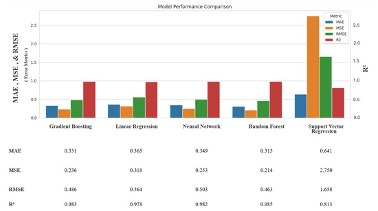
Figure 8.
Model evaluation based on performance metrics.
Additionally, Neural Networks can perform well if the dataset is large enough. However, based on the obtained values of MAE and MSE, SVR captures a non-linear Relationship but may require hyperparameter tuning. And yet, these results highlight the significant potential of AI-driven approaches in predicting urban congestion within the Casablanca smart city context, particularly where conventional traffic planning methods are limited.
The Linear Regression model, while serving as a simple baseline, exhibited significant underfitting, with widely scattered predictions and patterned residuals indicating its inability to capture the nonlinear dynamics of urban traffic Figure 9. This is in line with findings that traditional methods often struggle with complex urban data [68], and that machine learning frequently outperforms linear regression in traffic prediction [69]. In contrast, the Random Forest Regressor demonstrated strong predictive power, characterized by tight clustering of predicted versus actual values, low bias residuals, and a clear, interpretable hierarchy of feature importance, making it robust and effective in handling complex nonlinear relationships Figure 10. Its performance and interpretability are supported by the results reported in [70,71], which identifies it as a promising non-linear method for traffic prediction with low errors observed [72].
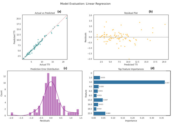
Figure 9.
Linear Regression Model Evaluation. (a) Actual vs Predicted: This is a scatter plot showing the observed target values (the Travel-Time Index) on the horizontal axis and the values predicted by the model on the vertical axis. The dashed line at 45° indicates perfect agreement, and how proximate the points are to this line reflects the overall predictive accuracy of the model in question. (b) Residual Plot: graph of the residuals (observed-predicted) versus the predicted values. The random distribution of points around zero, with no discernible pattern, demonstrates that the errors in the model are unbiased and homogeneous across the prediction range. (c) Prediction Error Distribution: A histogram of the residuals, overlaid with a kernel density estimate (KDE). The shape of the distribution (‘symmetry’ and ‘skewness’, for example) provides a concise summary of the magnitude and frequency of prediction errors for the model. (d) Top Feature Importances: A horizontal bar chart showing the most important input variables as identified by the model. These could be, for example, the mean decrease in impurity for tree-based models or the absolute coefficient values for linear models. The features are ordered by importance, from the most impactful to the least, allowing for a prompt visual evaluation of the predictors that drive the performance of the model.
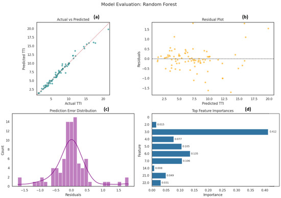
Figure 10.
Random Forest Model Evaluation. (a) Scatter plot of observed versus predicted target values. (b) Residuals (observed − predicted) plotted against the predicted values. (c) Histogram of the residuals overlaid with a kernel-density estimate. (d) Horizontal bar chart ranking the most influential input variables.
Similarly, the Gradient Boosting Regressor performed comparably to Random Forest, with slightly tighter fits in some regions and a nuanced ability to model subtle traffic patterns, though it showed minor susceptibility to overfitting if not carefully tuned Figure 11. Gradient Boosting is also recognized for strong travel time prediction aligned with the results obtained by [73].
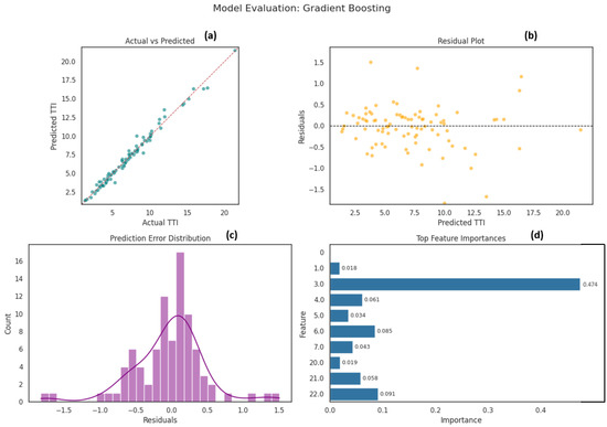
Figure 11.
Gradient Boosting Model Evaluation. (a) Scatter plot of observed versus predicted target values. (b) Residuals (observed − predicted) plotted against the predicted values. (c) Histogram of the residuals overlaid with a kernel-density estimate. (d) Horizontal bar chart ranking the most influential input variables.
According to the results obtained, the Neural Network (MLP Regressor) offered a decent fit but with greater scatter and higher residual variance than the ensemble methods, reflecting challenges in generalization and stability without extensive hyperparameter tuning; moreover, its lack of native interpretability limits practical insights Figure 12. Although MLP is positioned mid-ranked in this study, it yielded the lowest accuracy and F1-score in the experiment conducted by [70], in addition to requiring a relatively long training time due to its algorithmic complexity.
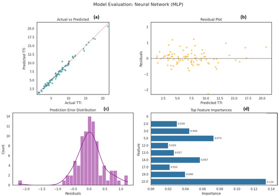
Figure 12.
Neural Network Model Evaluation. (a) Scatter plot of observed versus predicted target values. (b) Residuals (observed − predicted) plotted against the predicted values. (c) Histogram of the residuals overlaid with a kernel-density estimate. (d) Horizontal bar chart ranking the most influential input variables.
Finally, the Support Vector Regressor (SVR) delivered moderate performance with fair alignment yet sparser predictions and inconsistent residuals, particularly struggling at extreme congestion levels; combined with slower training and scalability issues, SVR proved less suitable for this complex forecasting task Figure 13. Despite SVR outperforming naive methods and performing well in stable conditions, there are clear limitations when it is used in highly variable contexts. This finding was further endorsed by the conclusion of [74] research study. Overall, ensemble methods, particularly Random Forest and Gradient Boosting, emerged as the most balanced and reliable models, effectively capturing the nonlinear and dynamic nature of traffic congestion while offering valuable interpretability. As shown in Table 2, the comparative evaluation of the five predictive models reveals distinct strengths and limitations in forecasting the Travel Time Index (TTI).
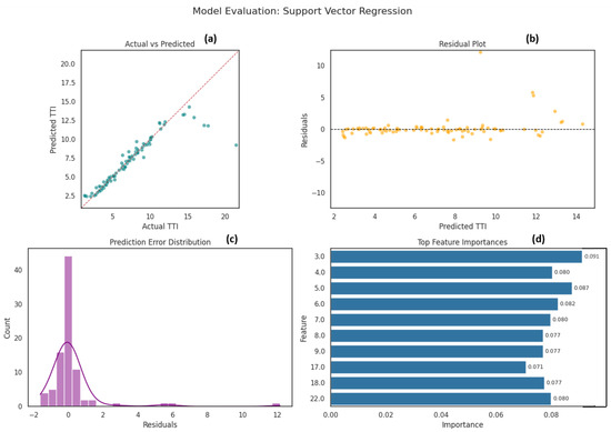
Figure 13.
SVR Model Evaluation. (a) Scatter plot of observed versus predicted target values. (b) Residuals (observed − predicted) plotted against the predicted values. (c) Histogram of the residuals overlaid with a kernel-density estimate. (d) Horizontal bar chart ranking the most influential input variables.

Table 2.
Model performance summary and comparison.
Hyperparameter Tuning of the Random Forest Model
To boost the performance of our best model, the Random Forest Regressor, we used GridSearchCV [75], from the Scikit-learn, the open-source machine learning library for the Python programming language [76], to fine-tune its key hyperparameters. This process tests different combinations of settings to find the best fit, improving accuracy and reducing overfitting. As can be seen from Table 3, we focused on parameters like the number of trees, tree depth, and sample requirements, using cross-validation to ensure reliable results. The best hyperparameters identified by GridSearchCV were then used to retrain the optimized Random Forest model on the full training set.

Table 3.
Key Hyperparameters Considered for Random Forest Tuning.
Optimized Random Forest Performance after the use of GridSearchCV is represented in Table 4:

Table 4.
Key Obtained Values Before and After Hyperparameters Tuning.
The optimized model showed better R2 and lower MAE/MSE compared to the baseline model, making it more reliable for predicting the Travel Time Index (TTI) in our selected case study. To sum up, Random Forest is considered the best overall performer (accuracy, stability, interpretability). The Gradient Boosting is also an excellent alternative with similar results, supporting their top rankings in the verdict. In summary, the insights provided in the verdict by the MAE, MSE, and R2 metrics mirror the qualitative assessment, as shown in Table 2.
While hyperparameter tuning significantly improves model performance, model selection must consider factors other than accuracy, such as computational speed and practical deployment feasibility. Indicative results from the literature demonstrate the promise of LSTM, a form of recurrent neural network built for sequential data that can learn long-term relationships in traffic data without requiring considerable feature engineering. However, related research in [68] found that LSTM models frequently require additional computing resources and a longer training time, which may restrict their real-time implementation in resource-constrained situations such as traffic management apps or platforms.
This was further substantiated in [77]. Moreover, the study’s findings further support the strengths and positive results of the proposed hybrid LSTM model, such as achieving high prediction accuracy in terms of RMSE and R2. The deep learning model could encounter some computational complexity, especially those combining CNN and LSTM, which can be computationally intensive in terms of computational cost, training time, or resource requirements. This, in turn, could be a practical limitation for real-time deployment in resource-constrained environments. Instead, suggested models such as Random Forest and Gradient Boosting offer a balanced combination of high predictive accuracy, low computational cost, and interpretability through feature importance analysis. This makes them more appropriate for actual deployment.
4.5. Practical Implications and Future Applications
The predictive model presented in this research paper was methodically constructed on Waze crowd-sourced data, which captures only travel times for motor vehicles on the road network. Nevertheless, the foundational methodology, including spatio-temporal feature engineering, machine learning regression with hyperparameter optimization, and model evaluation using MAE, MSE, RMSE, and R2, can be extended to other transport modes like walking, cycling, rail, and public transit transport services, provided that appropriate travel time observations are available.
- For non-motorized users (pedestrians and cyclists), the principal data sources are GPS-based crowd-sourced mobility apps that can generate travel-time indices. These datasets can be cleaned and aggregated to produce a Pedestrian TTI (TTIP)/Cyclist TTI (TTIC) analogous to the initial TTI. Pedestrian and cycling speeds are highly sensitive to environmental factors (weather conditions, steepness of a road, elevation, material and surface quality of the cycle paths, and sidewalk width). These additional covariates can be derived from sources like Digital Elevation Model (DEM) and OpenStreetMap (OSM) tags, which will help our high-performing predictive models (Random Forest and Gradient Boosting) retain strong predictive power if incorporated into the feature set.
- Rail, tram, and bus services generate structured timetabling information that can be accessed through the open data portals of the Moroccan National Railways Office (ONCF) and the tram/bus operators. By merging scheduled departure/arrival times with real-time vehicle location data, a Transit Travel Time Index (TTITr) can be calculated for each line segment, as with the road-based TTI. Since rail and bus networks are less dense than the road network, the model’s temporal granularity can be adjusted without loss of predictive accuracy. Moreover, passenger load information (available from ticket validation systems) can be introduced as an additional predictor to capture congestion-related delays.
- The adaptation involves data acquisition and preprocessing, feature engineering with mode-specific variables, retraining the model using the expanded dataset with additional covariates, and finally computing the same performance evaluation metrics (KPIs: MAE, MSE, RMSE, and R2). By following this method/workflow, our AI-driven framework can be generalized to cover the full modal split in the city of Casablanca.
Thus, this extension not only broadens its applicability but also provides direction for future work that will help to implement and validate the proposed approach, allowing city planners to monitor and predict congestion across the entire urban mobility system, not solely the motorized component.
While Casablanca currently lacks an intelligent traffic management system capable of reducing predicted congestion in critical corridors during peak hours, even though its existing traffic light system operates automatically on fixed schedules. The predictive Travel Time Index (TTI) model developed in this research can complement this by providing a more user-oriented service that can be implemented directly on users’ devices. This could be achieved by integrating it into a dedicated mobile app or navigation app, enabling travelers to access forecasted TTI values for their intended routes. Another option would be to deploy the model as a cloud-based API service, where users’ devices can send travel queries and receive real-time congestion forecasts. This setup would enable commuters to take proactive and prospective actions, allowing them to choose the best itinerary before starting their trips. This implementation would align with Casablanca’s current mobility infrastructure, empowering everyday commuters in the city with actionable congestion insights.
In addition to the temporal variables that guide the model predictions, the socio-economic aspect of each commune plays an important role in explaining the observed spatial heterogeneity of the TTI. The congestion levels measured by the Travel-Time Index (TTI) are considerably influenced by the existing built environment of each Casablanca commune. It is evident that communes with higher population size and density generate more vehicle-kilometers, which in turn raises demand on the road network and increases the hourly TTI, especially during the observed peak periods. However, land use composition moderates this demand: an expanded residential area typically generates more frequent travel, while larger industrial and commercial zones concentrate shipments and delivery activities, contributing to increased traffic and extended wait times for trucks. The availability of parking areas has also been demonstrated to influence driver behavior; the limited availability of car parks forces more drivers to circulate while searching for parking spaces, therefore resulting in higher TTI values. Public transport infrastructure has a positive effect on the transport system: communes that host a greater number of tram stations (71 stations across 12 communes) and bus stops (732 stops on 970 km of routes) provide travel alternatives to private cars, which can reduce the number of car journeys and reduce congestion. The types and length of roads are also important: communes served by primary and secondary roads experience higher capacity constraints than those with extensive highway segments, because the highways allow higher flow rates and reduce traffic jams. Integration of socio-economic and infrastructural variables within the proposed predictive model will facilitate a comprehensive understanding of the spatial heterogeneity in TTI across Casablanca and identify the most effective urban planning solutions for addressing congestion.
5. Conclusions
This study aimed to predict the Travel Time Index (TTI) in Casablanca through a comparative analysis of neural network and multiple machine learning models. Among the models evaluated, Random Forest demonstrated the most consistent and balanced performance. It excelled in terms of accuracy, robustness, and interpretability, which all serve to ensure the success of policy-oriented applications. Gradient boosting also yielded highly competitive results, though it was considerably more susceptible to hyperparameter tuning. Linear Regression and Support Vector Regression (SVR) served as useful baselines but were less effective under dynamic traffic conditions. The Multilayer Perceptron (MLP) neural network revealed moderate success but required extensive calibration and lacked interpretability, which constrains its practical use in mobility planning. A significant contributing factor to the elevated performance of the RF model was the implementation of hyperparameter tuning techniques. The employment of strategies such as grid search and cross-validation was found to be essential for adapting the model to the specific characteristics of Casablanca’s traffic data, thus ensuring optimal effectiveness. This systematic optimization of input parameters has been demonstrated to achieve substantial enhancement in model accuracy while mitigating the occurrence of overfitting and improving the model’s capacity for generalization to unseen data. This optimization led to a notable improvement in model performance, with MAE reducing from 0.315 to 0.220, MSE decreasing from 0.214 to 0.123, and R2 increasing from 0.985 to 0.988, demonstrating not only the impact of tuning but also more efficient and reliable model development. The decision to base this analysis on a one-week, 24/7 time-series of TTI is an intentional methodological strength rather than a limitation. This focused time period captures all urban mobility patterns, from weekday commutes to the weekend, ensuring that all periodicities relevant for training models are represented while the effects of long-term urban changes are reduced. A noteworthy strength is that the crowd-sourced nature of Waze data ensures ecological validity, offering an authentic reflection of real-world traffic dynamics.
In conclusion, this research highlights the importance of AI-powered predictive tools in modern urban governance and policymaking, advocating for their continued development and deployment in smart city mobility systems. To improve models, future work should build upon this validated approach by aggregating larger datasets that capture longer and extended temporal periods and non-motorized modes, without methodological changes. This would facilitate a more comprehensive examination of seasonal variations (multi-seasonal data), weekly averaged TTI trends and evolving traffic patterns. This would enrich the understanding of urban traffic dynamics and enhance the robustness of predictive frameworks. Future research directions, in addition, involve exploring hybrid deep learning architectures and creating interactive dashboards to deliver real-time predictive insights to urban planners, stakeholders, and citizens, fostering more responsive and sustainable urban transportation ecosystems.
Author Contributions
Conceptualization, N.M. (Nessrine Moumen); methodology, N.M. (Nessrine Moumen); software, N.M. (Nessrine Moumen); validation, N.M. (Nessrine Moumen), H.B., N.M. (Nisrine Makhoul) and J.C.; formal analysis, N.M. (Nessrine Moumen); investigation, N.M. (Nessrine Moumen); resources, N.M. (Nessrine Moumen); data curation, N.M. (Nessrine Moumen); writing—original draft preparation, N.M. (Nessrine Moumen); writing—review and editing, N.M. (Nessrine Moumen), H.B. and N.M. (Nisrine Makhoul); visualization, N.M. (Nessrine Moumen); supervision, H.B., J.C. and N.M. (Nisrine Makhoul); project administration, N.M. (Nessrine Moumen) All authors have read and agreed to the published version of the manuscript.
Funding
This research received no external funding.
Data Availability Statement
The data supporting the findings of this study are available from the corresponding author upon request.
Conflicts of Interest
The authors declare no conflicts of interest.
Abbreviations
The following abbreviations are used in this manuscript:
| AI | Artificial Intelligence |
| ITS | Intelligent Transportation Systems |
| TTI | Travel Time Index |
| MLR | Multivariate Linear Regression |
| RF | Random Forest |
| MLP | Multilayer Perceptron |
| SVR | Support Vector Regression |
| MAE | Mean Absolute Error |
| MSE | Mean Squared Error |
| RMSE | Root Mean Squared Error |
| R2 | R-squared |
| ARIMA | Auto-Regressive Integrated Moving Average |
| HA | Historical Averages |
| ML | Machine learning |
| DL | Deep Learning |
| LSTM | Long Short-Term Memory |
| CNN | Convolutional Neural Networks |
| RNNs | Recurrent Neural Networks |
| HCP | Higher Planning Commission |
| API | Application Programming Interface |
| GIS | Geographic Information System |
| IDW | Inverse Distance Weighted |
| ONCF | National Railways Office |
| OSM | OpenStreetMap |
| DEM | Digital Elevation Model |
| TTIP | Pedestrian TTI |
| TTIC | Cyclist TTI |
| TTITr | Transit Travel Time Index |
| SUMP | Sustainable Urban Mobility Plan |
| IQR | Interquartile Range Method |
References
- Population Reference Bureau. Urbanization Rate by Continent 2025. prb.org. Available online: https://www.statista.com/statistics/270860/urbanization-by-continent/ (accessed on 9 May 2025).
- United Nations, Department of Economic and Social Affairs, Population Division. Urban Population by Country (1950 and 2024 Comparison). Available online: https://worldostats.com/country-stats/urban-rural-population-by-country/ (accessed on 9 June 2025).
- Babaei, A.; Khedmati, M.; Jokar, M.R.A.; Tirkolaee, E.B. Sustainable transportation planning considering traffic congestion and uncertain conditions. Expert Syst. Appl. 2023, 227, 119792. [Google Scholar] [CrossRef]
- World Bank; United Nations Department of Economic and Social Affairs (UN DESA). Africa: Urbanization Rate by Country 2023. Available online: https://databank.worldbank.org (accessed on 9 June 2025).
- United Nations Population Division. World Urbanization Prospects: 2018 Revision. Available online: https://population.un.org/wup/assets/WUP2018-Report.pdf (accessed on 29 May 2025).
- Higher Planning Commission (HCP)-Morocco. Main Results of General Population and Housing Census. Rabat, Dec. 2024. Available online: https://www.hcp.ma/file/242665/ (accessed on 2 July 2025).
- Mitieka, D.; Luke, R.; Twinomurinzi, H.; Mageto, J. Smart Mobility in Urban Areas: A Bibliometric Review and Research Agenda. Sustainability 2023, 15, 6754. [Google Scholar] [CrossRef]
- Du, S.; Li, T.; Gong, X.; Horng, S.-J. A Hybrid Method for Traffic Flow Forecasting Using Multimodal Deep Learning. Int. J. Comput. Intell. Syst. 2020, 13, 85–97. [Google Scholar] [CrossRef]
- Wan, J.; Li, D.; Zou, C.; Zhou, K. M2M Communications for Smart City: An Event-Based Architecture. In Proceedings of the 2012 IEEE 12th International Conference on Computer and Information Technology (CIT), Chengdu, China, 27–29 October 2012; pp. 895–900. [Google Scholar] [CrossRef]
- Xu, H.; Berres, A.; Yoginath, S.B.; Sorensen, H.; Nugent, P.J.; Severino, J.; Tennille, S.A.; Moore, A.; Jones, W.; Sanyal, J. Smart Mobility in the Cloud: Enabling Real-Time Situational Awareness and Cyber-Physical Control Through a Digital Twin for Traffic. IEEE Trans. Intell. Transp. Syst. 2023, 24, 3145–3156. [Google Scholar] [CrossRef]
- Gohil, J.; Chauhan, Y.; Nimavat, D. Smart Traffic Management Using Transfer Learning Approach for Improve Urban Mobility. Int. J. Sci. Res. Comput. Sci. Eng. Inf. Technol. 2024, 10, 156–164. [Google Scholar] [CrossRef]
- Xu, Z.; Shahraki, A.S.; Rudolph, C. Blockchain-Based Malicious Behaviour Management Scheme for Smart Grids. Smart Cities 2023, 6, 3005–3031. [Google Scholar] [CrossRef]
- Sajadi, P.; Qorbani, M.; Moosavi, S.; Hassannayebi, E. Accident Impact Prediction Based on a Deep Convolutional and Recurrent Neural Network Model. Urban Sci. 2025, 9, 299. [Google Scholar] [CrossRef]
- Berres, A.; Moriano, P.; Xu, H.; Tennille, S.; Smith, L.; Storey, J.; Sanyal, J. A traffic accident dataset for Chattanooga, Tennessee. Data Brief. 2024, 55, 110675. [Google Scholar] [CrossRef]
- Alqhatani, M.; Setunge, S.; Mirodpour, S. Can a polycentric structure affect travel behaviour? A comparison of Melbourne, Australia and Riyadh, Saudi Arabia. J. Mod. Transp. 2014, 22, 156–166. [Google Scholar] [CrossRef]
- Bhaskara, J.A.; Nurmandi, A. Role of Artificial Intelligence in the Smart City: A Bibliometric Review. In Communications in Computer and Information Science; Springer Science and Business Media Deutschland GmbH: Berlin/Heidelberg, Germany, 2022; pp. 589–596. [Google Scholar] [CrossRef]
- Kirimtat, A.; Krejcar, O.; Kertesz, A.; Tasgetiren, M.F. Future Trends and Current State of Smart City Concepts: A Survey. IEEE Access 2020, 8, 86448–86467. [Google Scholar] [CrossRef]
- Prawiyogi, A.G.; Purnama, S.; Meria, L. Smart Cities Using Machine Learning and Intelligent Applications. Int. Trans. Artif. Intell. 2022, 1, 102–116. [Google Scholar] [CrossRef]
- Jiang, H.; Geertman, S.; Witte, P. The contextualization of smart city technologies: An international comparison. J. Urban Manag. 2022, 12, 33–43. [Google Scholar] [CrossRef]
- Lee, S.; Yang, J.; Cho, K.; Cho, D. The Influence of Transportation Accessibility on Traffic Volumes in South Korea: An Extreme Gradient Boosting Approach. Urban Sci. 2023, 7, 91. [Google Scholar] [CrossRef]
- Yusuf, O.; Rasheed, A.; Lindseth, F. Leveraging Big Data and AI for Sustainable Urban Mobility Solutions. Urban Sci. 2025, 9, 301. [Google Scholar] [CrossRef]
- Pali, P.; Verma, S.; Patel, A.; Pathak, V.; Soni, V. Intelligent Urban Transportation Systems (Iuts): A Survey of AI-Driven Innovations and Future Directions. Int. J. Innov. Res. Sci. Eng. Technol. 2023, 12, 8068–8073. [Google Scholar] [CrossRef]
- Ang, L.; Iwami, M.; Chen, Y.; Du, Z.; Liu, B.; Wang, F. A Systematic Review of Urban Design and Computer Modelling Methods to Support Smart City Development in a Post-COVID Era. Lect. Notes Civ. Eng. 2023, 211, 1234–1246. [Google Scholar] [CrossRef]
- Aljuaydi, F.; Wiwatanapataphee, B.; Wu, Y.H. Multivariate machine learning-based prediction models of freeway traffic flow under non-recurrent events. Alex. Eng. J. 2022, 65, 151–162. [Google Scholar] [CrossRef]
- Liyanage, S.; Abduljabbar, R.; Dia, H.; Tsai, P.-W. AI-based neural network models for bus passenger demand forecasting using smart card data. J. Urban Manag. 2022, 11, 365–380. [Google Scholar] [CrossRef]
- Li, Y.; Zhao, W.; Fan, H. A Spatio-Temporal Graph Neural Network Approach for Traffic Flow Prediction. Mathematics 2022, 10, 1754. [Google Scholar] [CrossRef]
- Jilani, U.; Asif, M.; Zia, M.Y.I.; Rashid, M.; Shams, S.; Otero, P. A Systematic Review on Urban Road Traffic Congestion. Wirel. Pers. Commun. 2023, 140, 81–109. [Google Scholar] [CrossRef]
- Pramanik, A.; Rahman, M.; Anam, A.S.M.I.; Ali, A.A.; Amin, M.A.; Rahman, A.K.M.M. Modeling Traffic Congestion in Developing Countries using Google Maps Data. arXiv 2020, arXiv:2011.02359. [Google Scholar]
- Kashyap, A.A.; Raviraj, S.; Devarakonda, A.; K, S.R.N.; V, S.K.; Bhat, S.J. Traffic flow prediction models—A review of deep learning techniques. Cogent Eng. 2021, 9, 1–24. [Google Scholar] [CrossRef]
- Moriano, P.; Berres, A.; Xu, H.; Sanyal, J. Spatiotemporal features of traffic help reduce automatic accident detection time. Expert Syst. Appl. 2023, 244, 122813. [Google Scholar] [CrossRef]
- Liu, T.; Meidani, H. Graph neural networks for travel distance estimation and route recommendation under probabilistic hazards. Int. J. Transp. Sci. Technol. 2025. [Google Scholar] [CrossRef]
- Khalifa, A.; Idsouguou, Y.; Benabbou, L.; Zirari, M. Machine Learning Approaches for Traffic Volume Forecasting: A Case Study of the Moroccan Highway Network. arXiv 2017, arXiv:1711.06779. [Google Scholar] [CrossRef]
- Bibri, S.E.; Allam, Z. The Metaverse as a virtual form of data-driven smart cities: The ethics of the hyper-connectivity, datafication, algorithmization, and platformization of urban society. Comput. Urban Sci. 2022, 2, 1–22. [Google Scholar] [CrossRef]
- Lukic Vujadinovic, V.; Damnjanovic, A.; Cakic, A.; Petkovic, D.R.; Prelevic, M.; Pantovic, V.; Stojanovic, M.; Vidojevic, D.; Vranjes, D.; Bodolo, I. AI-Driven Approach for Enhancing Sustainability in Urban Public Transportation. Sustainability 2024, 16, 7763. [Google Scholar] [CrossRef]
- Zhang, T.; Xu, J.; Cong, S.; Qu, C.; Zhao, W. A Hybrid Method of Traffic Congestion Prediction and Control. IEEE Access 2023, 11, 36471–36491. [Google Scholar] [CrossRef]
- Bibri, S.E.; Krogstie, J. The emerging data–driven Smart City and its innovative applied solutions for sustainability: The cases of London and Barcelona. Energy Inform. 2020, 3, 5. [Google Scholar] [CrossRef]
- Makhoul, N. Review of data quality indicators and metrics, and suggestions for indicators and metrics for structural health monitoring. Adv. Bridg. Eng. 2022, 3, 1–32. [Google Scholar] [CrossRef]
- Makhoul, N. Bayesian Decision-Making Process Including Structural Health Monitoring Data Quality for Bridge Management. KSCE J. Civ. Eng. 2024, 28, 2818–2835. [Google Scholar] [CrossRef]
- Yang, L.; Shami, A. On hyperparameter optimization of machine learning algorithms: Theory and practice. Neurocomputing 2020, 415, 295–316. [Google Scholar] [CrossRef]
- Vemuri, S.; François-Jacobs, É.; Ambrosino, G.; González, N.C.; Gómez, M.; Bochinska, Z.; Baffi, S.; Boudet, L.; Heitplatz, A.; Almendros Salerno, A. MobiliseYourCity Global Monitor 2025—Factsheet: Casablanca, Morocco. Available online: www.mobiliseyourcity.net (accessed on 17 July 2025).
- Waze Data API. Waze for Cities: Your Partner for Mobility. Available online: https://www.waze.com/fr/wazeforcities (accessed on 8 November 2024).
- Kendall, K.M.; Stuart, A. The Advanced Theory of Statistics. Vol.3: Design and Analysis, and Time-Series. Griffin. (A Classic Text Covering Foundational Statistical Methods). ats. 1976, Volume 3. Available online: https://ui.adsabs.harvard.edu/abs/1976ats..book.....K/abstract (accessed on 19 July 2025).
- James, G.; Witten, D.; Hastie, T.; Tibshirani, R. An Introduction to Statistical Learning, 2nd ed.; Springer: New York, NY, USA, 2021; ISBN 9781071614174. [Google Scholar]
- Breiman, L. Random forests. Mach. Learn. 2001, 45, 5–32. [Google Scholar] [CrossRef]
- Sideris, N.; Bardis, G.; Voulodimos, A.; Miaoulis, G.; Ghazanfarpour, D. Using Random Forests on Real-World City Data for Urban Planning in a Visual Semantic Decision Support System. Sensors 2019, 19, 2266. [Google Scholar] [CrossRef]
- Rodriguez-Galiano, V.F.; Ghimire, B.; Rogan, J.; Chica-Olmo, M.; Rigol-Sanchez, J.P. An assessment of the effectiveness of a random forest classifier for land-cover classification. ISPRS J. Photogramm. Remote Sens. 2012, 67, 93–104. [Google Scholar] [CrossRef]
- Mutale, B.; Withanage, N.C.; Mishra, P.K.; Shen, J.; Abdelrahman, K.; Fnais, M.S. A Performance Evaluation of Random Forest, Artificial Neural Network, and Support Vector Machine Learning Algorithms to Predict Spatio-Temporal Land Use-Land Cover Dynamics: A Case from Lusaka and Colombo. Front. Environ. Sci. 2024, 12, 1431645. [Google Scholar] [CrossRef]
- Louppe, G.; Wehenkel, L.; Sutera, A.; Geurts, P. Understanding variable importances in forests of randomized trees. In Advances in Neural Information Processing Systems; Burges, C.J., Bottou, L., Welling, M., Ghahramani, Z., Weinberger, K.Q., Eds.; Curran Associates, Inc.: Red Hook, NY, USA, 2013; Available online: https://proceedings.neurips.cc/paper_files/paper/2013/file/e3796ae838835da0b6f6ea37bcf8bcb7-Paper.pdf (accessed on 20 July 2025).
- Chen, T.; Guestrin, C. XGBoost: A Scalable Tree Boosting System. In Proceedings of the 22nd ACM SIGKDD International Conference on Knowledge Discovery and Data Mining (KDD ‘16), San Francisco, CA, USA, 13–17 August 2016; pp. 785–794. [Google Scholar] [CrossRef]
- Natekin, A.; Knoll, A. Gradient boosting machines, a tutorial. Front. Neurorobotics. 2013, 7, 21. [Google Scholar] [CrossRef]
- Rumelhart, D.E.; Hinton, G.E.; Williams, R.J. Learning representations by back-propagating errors. Nature 1986, 323, 533–536. [Google Scholar] [CrossRef]
- LeCun, Y.; Bengio, Y.; Hinton, G. Deep learning. Nature 2015, 521, 436–444. [Google Scholar] [CrossRef] [PubMed]
- Heaton, J. Ian Goodfellow, Yoshua Bengio, and Aaron Courville: Deep learning. Genet. Program. Evolvable Mach. 2017, 19, 305–307. [Google Scholar] [CrossRef]
- Vapnik, V.N. (Ed.) Introduction: Four Periods in the Research of the Learning Problem. In The Nature of Statistical Learning Theory; Springer: New York, NY, USA, 2000; pp. 1–15. [Google Scholar] [CrossRef]
- Drucker, H.; Burges, C.J.C.; Kaufman, L.; Smola, A.; Vapnik, V.N. Support Vector Regression Machines. In Proceedings of the Advances in Neural Information Processing Systems (NIPS), Denver, CO, USA, 2–5 December 1996; Mozer, M.C., Jordan, M., Petsche, T., Eds.; Morgan Kaufmann: San Mateo, CA, USA; MIT Press: Cambridge, MA, USA, 1997; Volume 9, pp. 155–161. Available online: https://proceedings.neurips.cc/paper_files/paper/1996/file/d38901788c533e8286cb6400b40b386d-Paper.pdf (accessed on 12 February 2025).
- Smola, A.J.; Schölkopf, B. A tutorial on support vector regression. Stat. Comput. 2004, 14, 199–222. [Google Scholar] [CrossRef]
- Bishop, C.M. Pattern Recognition and Machine Learning; Springer: Singapore, 2006. [Google Scholar]
- Rouky, N.; Bousouf, A. Dataset for Traffic Analysis in Casablanca, Morocco. Mendeley Data 2023, 1. [Google Scholar] [CrossRef]
- Rouky, N.; Bousouf, A.; Benmoussa, O.; Fri, M. A spatiotemporal analysis of traffic congestion patterns using clustering algorithms: A case study of Casablanca. Decis. Anal. J. 2024, 10, 100404. [Google Scholar] [CrossRef]
- Texas A&M Transportation Institute. 2023 Urban Mobility Report; Texas A&M Transportation Institute: Austin, TX, USA, 2024; Available online: https://static.tti.tamu.edu/tti.tamu.edu/documents/umr/archive/mobility-report-2023.pdf (accessed on 6 May 2025).
- Schrank, D.L.; Lomax, T.; Texas A&M Transportation Institute. The 2005 Urban Mobility Report; Texas A&M Transportation Institute: Austin, TX, USA, 2005. Available online: https://rosap.ntl.bts.gov/view/dot/61838 (accessed on 6 May 2025).
- Dorosan, M.; Dailisan, D.; Valenzuela, J.F.; Monterola, C. Use of machine learning in understanding transport dynamics of land use and public transportation in a developing city. Cities 2023, 144, 104587. [Google Scholar] [CrossRef]
- Makhoul, N.; Derras, B. Machine Learning Improving Seismic Infrastructure Recovery Time Estimation. In Bridge Maintenance, Safety, Management, Digitalization and Sustainability; Casas, J.R., Frangopol, D.M., Turmo, J., Eds.; CRC Press: London, UK, 2024; pp. 3276–3285. [Google Scholar] [CrossRef]
- Bajaj, M.R.; Kumar, N.-R. A Research Paper on AI for Traffic Management. Available online: https://doi.org/10.13140/RG.2.2.21119.69287 (accessed on 9 April 2025).
- Ma, C. Smart city and cyber-security; technologies used, leading challenges and future recommendations. Energy Rep. 2021, 7, 7999–8012. [Google Scholar] [CrossRef]
- Moumen, N.; Radoine, H.; Nahiduzzaman, K.M.; Oulidi, H.J. Smartainity: A Comprehensive Framework for Urban Performance Assessment in African Smart Cities with Key Performance Indicators. In Lecture Notes in Networks and Systems; Springer: Cham, Switzerland, 2024; Volume 931, pp. 126–138. [Google Scholar] [CrossRef]
- Moumen, N.; Radoine, H.; Nahiduzzaman, K.M.; Oulidi, H.J. Contextualizing the Smart City in Africa: Balancing Human-Centered and Techno-Centric Perspectives for Smart Urban Performance. Smart Cities 2024, 7, 712–734. [Google Scholar] [CrossRef]
- Rodrigues, F. On the Importance of Stationarity, Strong Baselines and Benchmarks in Transport Prediction Problems. In Proceedings of the 2023 IEEE 26th International Conference on Intelligent Transportation Systems (ITSC), Bilbao, Spain, 24–28 September 2023; pp. 4927–4932. [Google Scholar]
- Alomari, A.H.; Khedaywi, T.S.; Marian, A.R.O.; Jadah, A.A. Traffic speed prediction techniques in urban environments. Heliyon 2022, 8, e11847. [Google Scholar] [CrossRef] [PubMed]
- Feng, X.; Ahvar, E.; Lee, G.M. Evaluation of Machine Leaning Algorithms for Streets Traffic Prediction: A Smart Home Use Case. Sensors 2023, 23, 2174. [Google Scholar] [CrossRef] [PubMed]
- Razali, N.A.M.; Shamsaimon, N.; Ishak, K.K.; Ramli, S.; Amran, M.F.M.; Sukardi, S. Gap, techniques and evaluation: Traffic flow prediction using machine learning and deep learning. J. Big Data 2021, 8, 1–25. [Google Scholar] [CrossRef]
- Ashwini, B.P.; Sumathi, R.; Sudhira, H.S. Bus Travel Time Prediction: A Comparative Study of Linear and Non-Linear Machine Learning Models. J. Phys. Conf. Ser. 2022, 2161, 012053. [Google Scholar] [CrossRef]
- Sun, P.; Boukerche, A.; Tao, Y. SSGRU: A novel hybrid stacked GRU-based traffic volume prediction approach in a road network. Comput. Commun. 2020, 160, 502–511. [Google Scholar] [CrossRef]
- Bratsas, C.; Koupidis, K.; Salanova, J.-M.; Giannakopoulos, K.; Kaloudis, A.; Aifadopoulou, G. A Comparison of Machine Learning Methods for the Prediction of Traffic Speed in Urban Places. Sustainability 2019, 12, 142. [Google Scholar] [CrossRef]
- Zhao, Y.; Zhang, W.; Liu, X. Grid search with a weighted error function: Hyper-parameter optimization for financial time series forecasting. Appl. Soft Comput. 2024, 154, 111362. [Google Scholar] [CrossRef]
- Pedregosa, F.; Varoquaux, G.; Gramfort, A.; Michel, V.; Thirion, B.; Grisel, O.; Blondel, M.; Prettenhofer, P.; Weiss, R.; Dubourg, V.; et al. Scikit-learn: Machine Learning in Python. J. Mach. Learn. Res. 2011, 12, 2825–2830. Available online: http://scikit-learn.sourceforge.net (accessed on 27 July 2025).
- Li, X.; Wang, H.; Sun, P.; Zu, H. Spatiotemporal Features—Extracted Travel Time Prediction Leveraging Deep-Learning-Enabled Graph Convolutional Neural Network Model. Sustainability 2021, 13, 1253. [Google Scholar] [CrossRef]
Disclaimer/Publisher’s Note: The statements, opinions and data contained in all publications are solely those of the individual author(s) and contributor(s) and not of MDPI and/or the editor(s). MDPI and/or the editor(s) disclaim responsibility for any injury to people or property resulting from any ideas, methods, instructions or products referred to in the content. |
© 2025 by the authors. Licensee MDPI, Basel, Switzerland. This article is an open access article distributed under the terms and conditions of the Creative Commons Attribution (CC BY) license (https://creativecommons.org/licenses/by/4.0/).