Abstract
This paper presents a novel model for the year-round simulation of evapotranspiration (ET) and substrate temperature on two fundamentally different extensive green roof types: a conventional drainage-based “Economy Roof” and a retention-optimized “Retention Roof” featuring capillary water redistribution. The main scope is to bridge the gap in urban climate adaptation by providing a modeling tool that captures both hydrological and thermal functions of green roofs throughout all seasons, notably including periods with dormancy and low vegetation activity. A key novelty is the explicit and empirically validated integration of core physical processes—water storage layer coupling, explicit rainfall interception, and vegetation cover dynamics—with the latter strongly controlled by plant area index (PAI). The PAI, here quantified as the plant surface area per unit ground area using digital image analysis, directly determines interception capacity and vegetative transpiration rates within the model. This process-based representation enables a more realistic simulation of seasonal fluctuations and physiological plant responses, a feature often neglected in previous green roof models. The model, which can be fully executed without high computational power, was validated against comprehensive field measurements from a temperate climate, showing high predictive accuracy (R2 = 0.87 and percentage bias = −1% for ET on the Retention Roof; R2 = 0.91 and percentage bias = −8% for substrate temperature on the Economy Roof). Notably, the layer-specific coupling of vegetation, substrate, and water storage advances ecological realism compared to prior approaches. The results illustrate the model’s practical applicability for urban planners and researchers, offering a user-friendly and transparent tool for integrated assessments of green infrastructure within the context of climate-resilient city design.
1. Introduction
Urbanization and climate change have intensified the frequency and severity of flooding and heat events in cities. This development is largely driven by increased impervious surfaces and altered cycles of hydrology and energy. As a consequence, cities are increasingly affected by stormwater overload, elevated energy demands, and growing risks to public health during extreme weather events. Green roofs have emerged as nature-based solutions that mitigate these adverse impacts by enhancing stormwater retention, improving local microclimates, and reducing building energy demands, among other co-benefits [1,2,3,4].
In particular, retention-type green roofs—systems with enhanced water storage capacity—are now frequently implemented as stormwater management tools at both building and district scales. They are supposed to not only retain rainfall during extreme weather events but also to support aesthetic integrity and maintain healthy vegetation during summer months for continued cooling benefits [5,6]. Given that the use of potable water for irrigation is often limited or prohibited, understanding and predicting a green roof’s water consumption and cooling performance is essential for optimal design and function. From an urban planning perspective, the most important ecosystem services of green roofs are attractive appearance [4,6,7], cooling effect [8,9], increased urban biodiversity [10,11], and delaying runoff during precipitation events [12,13].
The hydrodynamic calculation of runoff delay is well documented in the literature [14,15,16] and one key input variable for these simulations is substrate moisture at the onset of a rain event, which strongly depends on evapotranspiration rates during prior dry periods. Similarly, evapotranspiration plays a decisive role in the thermal behavior of the roof by promoting latent heat loss, while substrate temperature governs sensible heat exchange between roof surfaces and the surrounding air. These two parameters—evapotranspiration and substrate temperature—therefore represent the most relevant calculable variables for evaluating both the hydrological performance and urban cooling capacity of green roofs. Their accurate prediction is essential to quantify retention capacity, guide irrigation strategies, and evaluate energy saving potential for green infrastructure planning [8,17,18,19].
Nevertheless, a review of existing modeling approaches reveals several persistent research gaps in the simulation of substrate temperature and evapotranspiration on green roofs. The summary in Table 1 presents a comparative analysis of eleven models which calculated both evapotranspiration and substrate temperature and were published between 1998 and 2021, highlighting the state of current modeling efforts. They have been reviewed regarding the calculation (Ca) and validation (Va) of soil moisture, stomatal resistance, interaction with drainage/retention layer, plant area index (PAI—the ratio of plant aboveground biomass to the substrate surface)/soil cover fraction (SCF—the ratio of plant cover of a measurement area), and interception, the simulation of which are important for a comprehensive model [20,21,22]. As well as regarding the validated ability to simulate a full year, having evapotranspiration measurements for result validation and no need for numeric solvers are necessary characteristics for a reliable and easy to use model, without the need of extensive computational power. While many studies address some of these aspects, no model provides a simulation with all the mentioned key parameters and characteristics.
One clear shortcoming across much of the existing literature is the limited validation of key variables, particularly interception, stomatal resistance, and the interaction between substrate and drainage or retention layers. While evapotranspiration is a central component of most models, only two (Takebayashi and Moriyama, 2007 [23]; Tabares-Velasco et al., 2012 [24]) include validation.
A second limitation is the underrepresentation of validated biophysical plant processes. Validated seasonal variation in plant parameters such as PAI and SCF, which are crucial for accurate modeling of evapotranspiration [25], remain largely underrepresented. Notable exceptions include the models by Tabares-Velasco et al. [25], de Munck et al. [26], and Decruz [27].
Overall, model usability remains a concern. Several modeling frameworks, especially those rooted in hydrodynamic or hygrothermal simulation, require extensive computational resources or the application of specialized software packages. Although these can provide high-resolution results, they are often impractical for implementation in daily use software for planners, engineers, or policymakers aiming to assess green roof scenarios in everyday applications. Models suitable for annual simulation with minimal computational effort are notably lacking in the reviewed literature.
Perhaps the most consistent omission among existing studies is the neglect of drainage and retention layer interactions. In many commercially available green roofs today, water flow is not limited to vertical percolation within the substrate. Lateral flows, capillary upward fluxes, and water storage in sub-layers significantly affect evapotranspiration dynamics and substrate thermal properties [20,22,28], yet none of the reviewed models explicitly represent this hydraulic coupling, limiting their capacity to capture the behavior of retention-optimized green roofs. In modern multilayered systems, this shortcoming becomes increasingly relevant for both hydrological and thermal modeling.
Finally, none of the models attempt full-year simulation with empirical validation against evapotranspiration. Instead, many studies focus on single seasons (typically summer) or isolated events, reducing the models’ ecological realism and generalizability.

Table 1.
Overview of models with calculation of evapotranspiration and substrate temperature comparing specific characteristics and key model parameters.
In summary, while notable progress has been made in individual aspects of green roof modeling, Table 1 illustrates that gaps remain in integrated, validated, and practically usable simulations of evapotranspiration and substrate temperature. Addressing these gaps—particularly the incorporation of vegetation dynamics, interception calculation, full-year applicability and drainage layer interaction—remains a key challenge and motivation for the development of more comprehensive models, such as the one proposed in the present study.
The overarching goals of this study are as follows:
- To model the two most essential variables—evapotranspiration and substrate temperature—with a high degree of accuracy, as they are fundamental for the prediction of the water use and energy performance of green roofs under changing weather conditions.
- To ensure usability and practicality, the model is designed to be applied with easily accessible input data, without requiring high computational resources, making it widely usable.
- To improve model accuracy by addressing key research gaps, specifically
- include interception calculation
- capture seasonal variation in PAI and SCF
- simulate and validate a full year
- include hydraulic coupling with drainage and retention layer
To achieve these aims, existing approaches are combined and refined into a model for green roof evapotranspiration and temperature, which is tested across representative green roof types. All simulations in this study were run using Microsoft Excel (Version 16.78 for Mac) to underscore its practical applicability without the need for advanced programming or simulation tools.
2. Materials and Methods
2.1. Study Site and Experimental Setup
For validation of the model, measurement data from the whole year of 2022 for two different green roof types, the so-called Economy Roof and Retention Roof, was used. The Economy Roof with its four layers (protection fleece, drainage mat, filter fleece, and substrate) is the most common standard build-up for extensive green roofs, at least for the German market and its neighboring countries [33,34]. The Retention Roof differs from the Economy Roof in its use of a water retention layer instead of a drainage layer and a capillary connection from this layer to the substrate. The measurements were carried out in previous studies [22,28] in the south of Germany, in Krauchenwies-Göggingen (48°0′20.27916″ N and 9°12′5.33952″ E) at an elevation of 623 m above sea level. This location falls within a warm temperature, fully humid warm summer climate classification [35]. The setup encompassed the two green roofs, each placed in a lysimeter with a surface area of 0.5 m2. As shown in Figure 1, the lysimeters were placed on a sealed surface. To minimize potential edge effects, e.g., an increased heat flux due to the sealed surface, a surrounding green roof was built for this experimental setup. Each green roof was equipped with sensors for leaf and air temperature at the vegetation level, substrate temperature, substrate moisture content, heat flux, outflow, and weight. Additionally, a weather station recorded precipitation, air temperature and relative humidity, wind speed, incoming shortwave solar irradiance, and incoming longwave radiation. A detailed list of the sensors, their location and their accuracy can be found in Table 2. The data was collected at intervals of 5 min, resulting in a dataset comprising 2 full years (1 April 2021 to 31 March 2023). The roof systems are distributed by Optigrün international AG, Krauchenwies-Göggingen, Germany and contain various roof layers (Figure 2). All experimental green roofs were fertilized with a slow-release fertilizer (Opticote, Optigrün international AG) at the beginning of the study period and were weeded approximately once per month in summertime to preserve the intended vegetation. The Economy Roof drains freely, while the discharge of the Retention Roof is restricted, as the drainage hole is positioned at 3 cm height. Further details about this research can be found in the corresponding publication by [28].
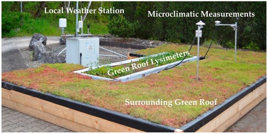
Figure 1.
Measurement site in Göggingen-Krauchenwies, Germany [28].
Table 2.
List of measured parameters, measurement devices used, approximate position of the sensors, and their accuracy.
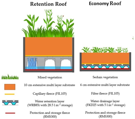
Figure 2.
Build-up from Gößner et al. [28] of the two different green roof systems modeled in this study.
The PAI, the SCF, and the interception capacity were also quantified. For the measurement of the vegetation cover and the PAI, triplicate photos were taken of each roof approximately once per week with a digital camera (D3200, Nikon, Düsseldorf, Germany and 8 mm/3.5 Fish-Eye II Lens Walimex pro, Studioexpress Vertriebs GmbH, Wiernsheim, Germany). The calculation of the vegetation cover and PAI was performed with the freeware CAN-EYE (INRAE, Paris, France).
The interception capacity quantifies the amount of rainfall retained on the surface of a plant’s above-ground biomass. Vegetation cover with high interception capacity can therefore improve a green roof system’s water retention capability. The assessment of interception capacity was based on Dunkerley and Booth [36], with minor adjustments to adapt to the smaller scale of our experiment. Ten low-growing perennials including herbaceous species and subshrubs commonly utilized for green roof installations were assessed. The initial preselection was based on a list of low-growing perennials suitable for green roofs and developed through years of practical experience, the final selection was determined by the availability at the nearest plant nursery. Of each species, three replicates were selected. To determine the interception capacity, a 10 × 10 cm frame was used to define the area covered by each plant’s aboveground biomass, and excess biomass outside this frame was trimmed. Then, the plant was cut just above the substrate, weighed, and placed in floral foam blocks to mimic the natural arrangement. Each plant was irrigated with 500 mL water for 30 s using a rainfall-tip nozzle. After two minutes, the plants were re-weighed to determine the interception capacity based on the weight difference, which was then extrapolated to 1 m2 and averaged for each plant species.
The water retention layer of the Retention Roof leads, in comparison to the Economy Roof, to highly increased soil moisture (17.18% higher on average), lower temperatures (4.2° cooler air at vegetation level on average during summer), and increased evapotranspiration (0.45 mm day−1 more evaporation on average). These different effects of the two green roofs are attributed to their differences in technical build-up. An evapotranspiration and substrate temperature model for green roofs should be able to model both types of green roofs.
2.2. Green Roof Model
As forecasting evapotranspiration is one of the main objectives of the model, and stomatal behavior plays a crucial role in the transpiration process, a detailed approach was chosen using the Penman–Monteith equation, which includes a dynamic calculation of stomatal resistance. In contrast, the simulation of substrate moisture, substrate temperature, and the capillary connection between the retention layer and the substrate was implemented in a more straightforward manner to avoid the need for computationally complex numerical solvers. A summary of all equations and constants used in the model is provided in Appendix A.
Stomatal behavior directly regulates plant transpiration activity. Previous research has shown that stomatal responses—and, consequently, transpiration rates—can vary significantly depending on environmental conditions [28,37,38]. For this reason, the stomatal resistance function is considered a key element for controlling transpiration and is particularly important for accurately computing the varying evapotranspiration rates associated with different green roof configurations.
The model requires the following meteorological input parameters: shortwave radiation, air temperature, precipitation, air humidity, and wind velocity. These parameters are freely available in Germany from a national network of weather stations. This data can be accessed via an open data server at the following link. User instructions are given in German and English: https://opendata.dwd.de/climate_environment/CDC/ (accessed on 26 August 2025).
2.2.1. Evaporation and Transpiration
In the model, interception and its evaporation is modeled explicitly, as a relevant part of small rain events can be retained at the plants’ surface [39,40]. Consequently, the original Penman–Monteith equation is only used to quantify the potential plant transpiration (TR).
where is the net radiation (), is the soil heat flux (), () represents the vapour pressure deficit (kPa) of the air, p is the atmospheric density (), is the specific heat capacity of the air (, is the psychrometric constant (kPa ), is the stomatal resistance (), and is the aerodynamic resistance ().
To determine the potential evaporation () for the interception storage, stomatal resistance restraint is eliminated from the Penman–Monteith equation [37].
In the model, stomatal resistance () determines the amount of transpiration as a function of solar radiation (f(solar)), air temperature (f(temp)), substrate water content (f(VWC)), and vapour pressure deficit (f(VPD)) [8]:
where is the minimum stomatal resistance (). The stomatal resistance varies between plant species. The lowest measured stomatal resistance for the prevailing plant (sedum spurium) on the Economy Roof was 336 , and 168 on the Retention Roof for sedum kamtschaticum [22].
The function of solar radiation has been suggested by Sailor [8], where is the solar radiation (W ). The function of the volumetric water content has been modified by Tabares-Velasco [25]. is the volumetric water content (), is the of the substrate at field capacity (), and is the of the substrate at the wilting point (). For the used substrate, is 0.06 m3 m−3 and is 0.455 m3 m−3. Both values were determined in the laboratory at TU Braunschweig. With a value of greater than 0.35 m3 m−3, the substrate meets the requirements of the FLL green roof guidelines [41].
For this study the function of vapor pressure deficit has been modified on an empirical basis, as the resulting restrain in transpiration was too high in relation to our measurements. Therefore, “+0.21” was added to the formula, which results, in general, in lower output values of the formula and thus increases the calculated evaporation.
es is the vapor pressure of the air at saturation (kPa) and ea the actual vapor pressure (kPa).
The function of temperature is based on Tabares-Velasco et al. [25], referring to leaf temperature. The original function does not consider temperatures below 0 °C. Since one aim of this work is to minimize the required computational power, the heat transfer of the vegetated area, including plant surface temperatures, is not calculated for reasons of simplicity. Instead, the air temperature (Ta) was used as an input parameter (K). As the model should be capable of modeling a whole year, the temperature function was modified to enable a calculation that includes negative air temperatures.
As the above mentioned parameters can vary quickly during the day [38], a model with relatively small time steps is necessary. In this study, the time step was 5 min.
To obtain the actual evaporation and transpiration of the vegetation the approach of Muzylo [42] is used:
where the actual evapotranspiration (ET in mm) consists of the actual evaporation of the interception storage (Ei in mm) and the actual transpiration of the plants (TR in mm). C is the amount of intercepted rainfall (mm) and interception storage and the maximum interception storage (mm).
As the green roof surface is normally not fully covered with vegetation, especially not the whole year, the bare substrate area is calculated separately from the plant covered area. Camillo and Gurney [43] suggested the following equation for describing the evaporation of the substrate ():
where is the water vapour density of the substrate () and the water vapour density of the air ().
Based on their own measurements, Tabares-Velasco, 2009 [37], suggested the following formula for the substrate surface resistance ():
For calculating the radiation budgets, formulae from the Food and Agriculture Organization (FAO) are used [44], modified for the use of time steps smaller than 24 h.
2.2.2. PAI
Based on measurements of the PAI (−) development on the economy and Retention Roof build-ups over the period of two years [22], the following empirical descriptions are used:
where the index e stands for economy, r stands for Retention Roof, and J is the number of the day of the year (.
Due to more available water and higher substrate thickness, the Retention Roof has denser vegetation (mean 5.04, SD 1.85) than the Economy Roof (mean 3.97, SD 0.87). The formula for the Economy Roof has a PBIAS of 7% and 9% for the Retention Roof, indicating a good model fit. However, the R2 values of 0.37 (Economy Roof) and 0.31 (Retention Roof) show that PAI calculation is only an approximation, as the PAI is strongly dependent on the prevailing environmental conditions.
2.2.3. Interception
is closely connected to PAI. According to the measured data, PAI strongly influences the interception capacity and plants with a high PAI tend to have a greater interception capacity (β = 0.356, SE = 0.05, p < 0.001, R2 = 0.91). Based on this data the empirical formula 15 (R2 = 0.76) describes the relationship between the PAI and for a PAI > 1 [22].
The water balance of the interception of the plant area is described as
where the rainfall N (mm) on the vegetated area consists of the actual evaporation of the interception storage (Ei in mm), the discharge from the storage (D in mm), and the change in the interception storage (C in mm).
2.2.4. Soil Cover Fraction
During measurements in a two-year period from [22], the SCF of both green roof types remained relatively stable, with a median of 0.96 for the Retention Roof and 0.9 of the Economy Roof (Figure 3).
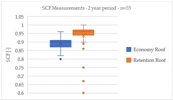
Figure 3.
Box-plot measurements of SCF.
2.2.5. Substrate
For simulating the substrate water content the following simple approach was employed, by adding the amount of precipitation falling directly on the substrate ( in mm), the discharge from the interception storage (D in mm), and the substrate resaturation amount to the water content (I in mm) and subtracting the evaporation from the substrate surface ( in mm), the water consumption for plant transpiration (TR in mm), and the discharge when the substrate is saturated ( in mm). As extensive green roofs with thin substrate thicknesses are modeled, the non-even distribution of the water content is neglected. is the substrate thickness (mm).
The substrate temperature is determined using a simple heat transfer equation based on [45]. The non-even distribution of the water content is neglected.
where is the substrate temperature (), the soil heat flux of the substrate (), the soil heat flux of the plants (), and the volumetric heat capacity of the substrate (). The basis for is and for , is reduced in dependency on the PAI.
2.2.6. Drainage and Substrate Resaturation
If the used drainage in the green roof has water storage, the water in this storage interacts with the substrate and the plants. Most water storages of green roofs have no capillary connection with the substrate. In this case the substrate gets moistened through water vapor processes. Some green roof types (Retention Roofs) though, have a capillary connection between water storage and substrate. In this case, the substrate gets saturated as long as there is water available [28]. Via the substrate resaturation velocity ( in mm period−1) in combination with the maximum substrate resaturation value ( in the two processes can be simulated by choosing empirical values. According to our 2-year measurements of the Retention Roof, for the maximum value of a period from 2 days after the last precipition until the next precipitation but with water in the retention/drainage layer was 0.41 m3 m−3. For the Economy Roof, was 0.23 m3 m−3. Via a comparison between measurements and simulation, was chosen in an iterative empirical way to match the measured substrate moisture behavior during periods without rain. For the Retention Roof, an of 0.005 mm 5 min−1 was determined, and for the Economy Roof an of 0.002 mm 5 min−1.
The drainage storage (Ds in mm) itself receives water from the substrate when the substrate is oversaturated (qs in mm) and loses water via discharge (qd in mm) when the drainage storage is full and due to the substrate resaturation process (I).
3. Results
3.1. Evapotranspiration Modelling
The model’s performance in predicting evapotranspiration (ET) was assessed seasonally and annually by comparing measured and simulated ET using R2, root mean square error (RMSE), and percentage bias (PBIAS) as statistical indicators (Table 3).
Table 3.
Evapotranspiration model performance based on coefficient of determination (R2), root mean square error (RMSE), and percentage bias (PBIAS).
Across the whole year, the Retention Roof model produced high predictive accuracy, with R2 values ranging from 0.80 to 0.96 across all seasons. The annual PBIAS of just −1% indicates an excellent overall fit and minimal systematic error. Daily mean ET was captured well throughout the year, except in April and May, where minor underestimations occurred, and in October, where ET was slightly overestimated (Figure 4a).
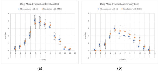
Figure 4.
Daily mean evaporation from 1 January to 12 December for (a) the Retention Roof and (b) the Economy Roof.
In contrast, the Economy Roof model performed well in spring and summer for the Economy Roof (R2 > 0.80) but showed a consistent overestimation of ET in autumn (especially in October) and underperformance in winter (R2 ≈ 0.52). The autumn overestimation is further confirmed by a PBIAS of 20% in those months, suggesting that senescence and reduced stomatal conductance in real plants may not be fully captured by the current parameterization. A pronounced seasonal trend is evident: the model tends to underestimate ET from January to May and overestimate it from June to December (Figure 4b). This behavior reflects an area where the model’s stomatal resistance function may not fully align with physiological adjustments of vegetation under variable irradiation, temperature, and substrate moisture combinations.
Despite structural and vegetative differences, both roofs showed good alignment in ET prediction during the active growing season, but the Retention Roof’s capillary water supply and thicker substrate enabled significantly higher ET, particularly under dry spells and warm conditions. On average, Retention Roof ET was 0.45 mm day−1 higher, aligning with prior field studies by Gößner et al. [28] and Cirkel et al. [20].
3.2. Substrate Temperature Modelling
Model accuracy in predicting substrate temperature varied clearly between roof types and seasons (Table 4).
Table 4.
Substrate temperature model performance based on coefficient of determination (R2), root mean square error (RMSE), and percentage bias (PBIAS).
For the Economy Roof, R2 ranged from 0.88 to 0.92 for spring through autumn, with a PBIAS of −5 to −1%, demonstrating a strong model fit. However, winter predictions were not accurate, likely due to the absence of freeze–thaw physics in the model (PBIAS—41%). The monthly daily mean temperature values, however, showed a very good fit for the total year (Figure 5b). Regarding the winter months, this may be coincidental.
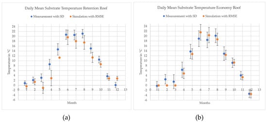
Figure 5.
Daily mean substrate temperature from 1 January to 12 December for (a) the Retention Roof and (b) the Economy Roof.
The model’s performance decreased substantially for the Retention Roof, especially during high substrate moisture and winter periods. Here, R2 dropped to 0.42. The monthly daily mean substrate temperatures were, apart from December, consistently underestimated (Figure 5a).
Looking at the measurement data over a period exceeding one month, Retention Roof substrate temperatures hovered just above 0 °C, suggesting frozen substrate, while the model, lacking phase-change functionality, simulated large daily amplitudes.
This deviation is a result of the simplified heat capacity calculation, which does not reflect the increased thermal inertia of wet or frozen substrates. Despite this, the model still demonstrated moderate predictive power during warm seasons (R2 = 0.42–0.82; PBIAS = −7 to −21%).
4. Discussion
4.1. Evaluation of Model Performance Relative to Study Goals
This study aimed to (1) accurately simulate ET and substrate temperature, (2) ensure the model’s year-round usability and low computational demand, and (3) improve model accuracy by addressing key research gaps. The degree to which each goal was achieved is discussed below.
4.1.1. Evapotranspiration
The model performed strongly in simulating daily mean ET, especially for the Retention Roof, which achieved seasonal regression coefficients of determination (R2) between 0.80 and 0.96 and annual PBIAS of just −1%. The strong agreement between measured and modeled ET behavior highlights the value of including substrate–drainage interactions, which are absent from other green roof models, especially for Retention Roof systems. Notably, the Retention Roof yielded higher ET rates than the Economy Roof, consistent with observed patterns from Gößner et al. [28], where thicker substrates and water availability extended transpiration phases.
For the Economy Roof, the model showed good agreement in spring and summer (R2 > 0.80) but had lower predictive power in winter (R2 ≈ 0.52) and significantly overestimated ET in autumn. This is likely due to the model’s lack of adequate adjustment for seasonal vegetation senescence. In addition, the measured and simulated maximum daily temperatures during September (mean daily max.) and October (mean daily max.), lay 0.72 °C higher than the long-term medium from 2002 to 2024 for September and 0.86 °C higher for October (based on DWD data, see Section 2.2). These high temperatures support a high transpiration rate in the model. However, this does not correspond with the actual behavior of the plants. Comparing the daily mean measurements and the modeled daily mean for the whole year, the Economy Roof shows a tendency for underestimation of the evaporation from January till May and an overestimation from June to December. Consequently, setting the restraints for transpiration in the model higher will lead to a better fit for the model from June to December, but to a significantly larger underestimation for January till May. This also indicates that the actual plant behavior is not yet fully described by the formulae used.
4.1.2. Substrate Temperature
Substrate temperature modeling proved more robust for the freely draining Economy Roof, indicating that the simplified heat capacity formulation is most reliable under moderate moisture content. Under saturated conditions, particularly in the Retention Roof during late winter, the model significantly underestimated temperatures. Looking at the data, the underestimation intensifies when the substrate moisture content is above 30%. Beneath high moisture content, the model is also not accurate when freezing occurs. This could be observed on the Retention Roof particularly during cold periods (January–March), where substrate temperatures were measured at ~0–2 °C, while the model simulated stronger diurnal fluctuations due to lacking phase change thermal dynamics. During months without freezing, substrate temperature was well predicted for the Economy Roof, with R2 ranging from 0.88 to 0.92 and PBIAS from −5 to −1%.
The constant underestimation when substrate moisture exceeded 30% suggests the need to establish a parameter for moisture-dependent thermal conductivity and heat capacity in future work—an approach not yet standard in most green roof models. To improve thermal prediction, future model extensions should take into account phase-change heat storage in wet substrates (e.g., via integration of freeze–thaw models), Moisture-dependent thermal conductivity, dynamic albedo shifts related to snow, or wet surface reflectance.
4.1.3. Year-Round Usability and Computational Efficiency
The model achieved full-year simulation with a 5 min resolution using Microsoft Excel, confirming its high practical usability and adaptability. This stands in contrast to many high-fidelity models often implemented in numerical solvers (e.g., HYDRUS-1D), which, while detailed, are not application friendly for planners and non-specialist stakeholders [26].
With no dependence on proprietary software or high-performance computing, this tool has a high suitability for integration in user software, with the ability to simulate both ET and substrate temperature jointly, including plant physiological effects.
4.1.4. Closing Knowledge Gaps in Process Representation
The most notable gap in previous models is the lack of comprehensive, year-round validation against measured ET data, with most studies either limited to summer periods or short events. By implementing continuous, multi-seasonal validation, the present model demonstrates robust year-round predictions especially for the Retention Roof, which achieved high R2 values across all seasons. This full-year validation offers a more nuanced understanding of temporal dynamics and systematic biases—such as the observed seasonal underestimation and overestimation patterns—which would be obscured in single-season or event-based studies.
Another substantial innovation is the explicit integration of drainage and retention layer interactions. All mentioned existing models simplify water movement to vertical percolation, neglecting the significant roles of lateral flows, capillary interactions, and water storage in sub-layers. Here, the model simulates these hydraulic couplings using empirical resaturation rates and maximum storage values derived from measurement data. Including these dynamics was pivotal in accurately predicting ET during dry periods.
Furthermore, this study incorporates year-round measurements of PAI and SCF, allowing empirical representation of seasonal vegetation shifts and their direct impact on interception and ET capacity. Such detailed vegetation parameters have rarely been implemented in previous green roof models, resulting in improved simulation of plant physiological responses (as evidenced by the close PAI/interception correlation, R2 = 0.91). Incorporating dynamic vegetation factors fills another gap, supporting recent findings on the importance of plant phenology for hydrological and thermal performance.
Another advancement is the integration of an explicit interception calculation within the model. Unlike most existing green roof models this model dynamically calculates interception based on measured PAI and soil cover fraction SCF. This allows for a realistic representation of rainfall intercepted by vegetation and substrate surfaces, a process that directly affects available water for ET and drainage. The integration of interception addresses a commonly overlooked process, thereby improving hydrological realism.
4.1.5. Comparative Model Performance in Literature Context
Compared to existing modeling studies, the performance of the presented model shows incremental improvements in some areas, particularly for ET on the Retention Roof, but also highlights where performance remains comparable to earlier work, especially regarding substrate temperature and ET on the Economy Roof (Table 5).
Table 5.
Model performance comparison.
For ET, the model achieves a strong correlation and low bias on the Retention Roof (R2 = 0.87, PBIAS = –1%), reflecting a real advancement in terms of year-round accuracy and balanced hydrological prediction. This level of performance exceeds the models by Feng (PBIAS 5–11%, R2 0.28–0.67) or Tabares (PBIAS –24% to +4%).
In contrast, the Economy Roof produces an R2 of 0.77 and a PBIAS of 22%, suggesting a moderate overestimation and a performance level comparable to the existing models of Feng (PBIAS 5–11%, R2 0.28–0.67) and Tabares (PBIAS –24% to +4%). While the incorporation of interception and layered retention processes represents a methodological improvement and a key reason for the good performance of the Retention Roof, these improvements did not translate into a clear overall gain in predictive accuracy.
For substrate temperature, the results are robust but not exceptional. The model achieves similar performance metrics to previously published approaches, particularly under warm and rather dry conditions. Comparable values reported by de Munck (R2 = 0.91; RMSE ≈ 4.3) and Tabares (RMSE ~2.0, PBIAS –4 to –6%) place the current model of the economy roof within the upper performance range, but not significantly beyond it.
In summary, the presented model stands out mainly through its process completeness and transparency, with unique features such as integrated interception modeling, dynamic vegetation inputs, and explicit retention-layer coupling. These advances show the models realism and reproducibility. However, in terms of quantitative performance—particularly for substrate temperature and ET on more simplified roof types—it achieves results broadly in line with existing models. The clearest gain is observed in hydrological performance on retention-optimized systems.
4.2. Limitations and Recommendations
While the presented model achieves robust performance in the simulation of ET—particularly on the retention roof—several limitations remain that underline necessities for future refinement.
Most notably, substrate temperature simulations under freezing and water-saturated conditions showed reduced accuracy, especially for the Retention Roof during winter months. This underperformance highlights the need to expand the thermal module by incorporating moisture-dependent thermal conductivity and heat capacity, as well as freeze-thaw dynamics and latent heat storage. These processes are crucial for replicating thermal buffering and phase-change effects, which are currently oversimplified.
In addition, it seems that vegetation dormancy transitions, particularly in late autumn, are not yet fully captured.
The transferability and reproducibility of the presented model are subject to climatic and contextual limitations. First, all measurements and model validations were conducted at a single temperate, humid site in southern Germany, which is characterized by distinct seasonal dynamics and a relatively uniform distribution of precipitation throughout the year. This means that part of the model equations and parameters, including vegetation development (PAI) and interception are calibrated for climates with moderate winters, warm summers, and sufficient rainfall. In regions with fundamentally different climatic conditions—such as arid zones with pronounced droughts, subtropical climates with highly seasonal rainfall, or areas with persistent snow cover in winter—processes may behave differently and require re-calibration or adaptation. Furthermore, the model is based on two specific green roof systems (Economy Roof and Retention Roof) that use substrate types, thicknesses, and plant species commonly found in the German and central European market, particularly drought-tolerant Sedum species. In other regions, alternative plant communities or substrate assemblies with different water retention and heat storage properties may influence the magnitude and timing of both ET and temperature regulation. It is therefore essential to locally validate vegetation parameters and substrate hydrophysical properties before applying the model in new contexts. Additionally, the field experiment was carried out on relatively small lysimeter surfaces under controlled edge conditions in a peri-urban environment. Larger roof areas, more complex urban settings, or significant variations in exposure, shading, or wind regimes could alter the local microclimate and influence the performance of green roof systems beyond the bounds tested here. Consequently, the direct transfer of the model to other geographic and climatic contexts must proceed with caution. Site-specific adjustments and empirical validation are recommended to ensure reliable model performance and reproducibility under different environmental boundary conditions.
4.3. Practical Implications
A key strength of the presented model is its low computational demand, enabling year-round simulations without the need for proprietary software or numerical solvers. This makes it particularly suitable for integration into urban planning software, where quick assessments and scenario evaluations are often required within constrained time and resource environments.
The model demonstrates how a mechanistically informed, yet accessible tool could support the evaluation and design of green infrastructure under variable and evolving climate conditions.
Of particular relevance is its scalability for use in climate-resilient infrastructure planning, where green roofs are increasingly recognized as multifunctional assets for water retention, thermal regulation, and biodiversity enhancement. The year-round simulation capability addresses the research gap illustrated before.
By also capturing the ET process of Retention Roofs the model is well-positioned for inclusion in forward-looking planning frameworks such as DWA-A 102-1 from the German association of water management, which promotes the integration of green roofs into water-sensitive and heat-adaptive strategies at both building and urban scales [47]. Moreover, the empirical basis of the model should facilitate reproducibility and foster trust among practitioners and decision-makers.
5. Conclusions
This study developed and empirically validated a new model to simulate year-round evapotranspiration and substrate temperature for two fundamentally different extensive green roof types. The model demonstrates very high accuracy for evapotranspiration on retention-optimized roofs, with an R2 value of 0.87 and a PBIAS of –1%, and for substrate temperature on conventional roofs, with an R2 of 0.91 and a PBIAS of –8%. Notable methodological advancements include the explicit integration of rainfall interception, dynamic modeling of plant canopies through PAI and SCF, and the simulation of water storage layer coupling—features that were absent in most prior models. Model performance proves robust across all seasons, and the approach can be implemented without relying on high computational power.
If incorporated into appropriate software tools, the model enables practitioners and planners to reliably predict the key hydrological and thermal functions of green roofs year-round, thereby supporting informed decisions in urban stormwater management and heat mitigation. Its low computational demand makes it especially applicable for routine planning and design in urban green infrastructure, corresponding to sector standards such as DWA-A 102-1.
Despite these strengths, some limitations remain: accuracy in substrate temperature simulation diminishes under freezing or fully saturated conditions, and estimates for evapotranspiration in conventional shallow roofs are less reliable during periods of plant dormancy. Consequently, further model improvements should aim to address freeze–thaw dynamics, moisture-dependent thermal properties, and vegetation dormancy and stress responses. In summary, the presented model closes key methodological gaps and is well suited for comprehensive assessment and design of green roofs in climate-resilient urban contexts. Future work should focus on extending its applicability to a broader range of climate zones and vegetation types, and on further refining the simulation of winter processes.
Funding
The data were collected as part of the Project “Building physics design of urban surfaces for a sustainable quality of life and environment in cities” which is 60% funded by the Federal Ministry of Education and Research BMBF (Grant Number: 01LR2022D). The remaining 40% was funded by Optigrün international AG.
Data Availability Statement
The raw data used for the analysis in this study can be provided on request by contacting the corresponding author.
Acknowledgments
We kindly acknowledge the permission of Optigrün international AG to use space for the experimental setup in the parking lot.
Conflicts of Interest
The author is an employee at the Optigrün international AG. The roof systems analyzed in this study are commercially available from Optigrün international AG, therefore, the funders had an influence on the choice of systems to be assessed. Still, all scientific standards were adhered to during the evaluation and processing of the data and the results are presented truthfully.
Abbreviations
The following abbreviations are used in this manuscript:
| Angstrom parameter | |
| seasonal correction factor | |
| Angstrom parameter | |
| cloud cover | |
| interception storage [mm] | |
| volumetric heat capacity air | |
| specific heat capacity air | |
| discharge interception storage [mm] | |
| drainage storage [mm] | |
| maximum drainage storage [mm] | |
| inverse earth-moon distance | |
| vapour pressure at saturation [kPa] | |
| actual vapour pressure [kPa] | |
| potential evaporation [mm] | |
| actual evaporation interception storage [mm] | |
| substrate evaporation [mm for Equation (17)] | |
| actual evapotranspiration [mm] | |
| soil heat flux | |
| soil heat flux plants | |
| Gsc | solar constant |
| soil heat flux substrate | |
| sensible heat flux density | |
| crop height [m] | |
| relative air humidity | |
| Substrate thickness [mm] [m for Equation (19)] | |
| Substrate resaturation [mm] | |
| Substrate resaturation velocity | |
| number of day of the year | |
| von Karman constant | |
| longitude [rad] | |
| longitude at center of time zone west of Greenwich [rad] | |
| Monin–Obukhov’s stability parameter | |
| measured sunshine duration [h] | |
| rainfall [mm] | |
| discharge drainage [mm] | |
| discharge substrate [mm] | |
| atmospheric pressure [kPA] | |
| atmospheric density | |
| water vapor density air | |
| water vapor density substrate | |
| saturated water vapor density | |
| aerodynamic resistance | |
| stomatal resistance | |
| minimum stomatal resistance | |
| substrate surface resistance | |
| plant area index | |
| plant area index Economy Roof | |
| plant area index Retention Roof | |
| outflow drainage layer [mm] | |
| substrate drainage [mm] | |
| extraterestric radiation [MJ ] | |
| Richardson number | |
| net radiation [MJ ] | |
| shortwave net radiation [MJ ] | |
| longwave net radiation [MJ ] | |
| solar radiation [W ] | |
| solar radiation at clear sky [W ] | |
| seasonal correction factor sun hours [h] | |
| maximum interception storage [mm] | |
| soil cover fraction | |
| Inverse soil cover fraction | |
| standard time mid period | |
| maximum daylight hours [h] | |
| sun hours per day [h] | |
| air temperature | |
| substrate temperature | |
| atmospheric transmission coefficient | |
| maximum air temperature during period [K] | |
| minimum air temperature during period [K] | |
| virtual temperature [K] | |
| actual transpiration [mm] | |
| potential Transpiration [mm] | |
| wind velocity | |
| vapor pressure deficit | |
| sun angle mid period [rad] | |
| sun angle start period [rad] | |
| sun angle end period [rad] | |
| sun hour angle [rad] | |
| height above sea level [m] | |
| height of air humidity measurements [m] | |
| height of wind velocity measurements [m] | |
| roughness length for sensible heat flux [m] | |
| roughness length for momentum [m] | |
| height of temperature measurements [m] | |
| albedo | |
| psychrometric constant | |
| sun angle [rad] | |
| atmospheric emissivity at clear sky | |
| substrate emissivity | |
| atmospheric stability parameter | |
| volumetric water content | |
| discharge substrate | |
| volumetric water content at field capacity | |
| volumetric water content at wilting point | |
| Maximum substrate resaturation | |
| extinction coefficient | |
| Stefan–Boltzmann constant | |
| latent evaporative heat | |
| heat flux atmospheric correction factor | |
| momentum atmospheric correction factor | |
| slope of the saturation–vapor–pressure temperature curve |
Appendix A
Table A1.
Summary of used equations.
Table A2.
Summary of all used constants.
References
- Santamouris, M. Heat Island Research in Europe: The State of the Art. Adv. Build. Energy Res. 2007, 1, 123–150. [Google Scholar] [CrossRef]
- Berardi, U. The Outdoor Microclimate Benefits and Energy Saving Resulting from Green Roofs Retrofits. Energy Build. 2016, 121, 217–229. [Google Scholar] [CrossRef]
- Rowe, D.B. Green Roofs as a Means of Pollution Abatement. Environ. Pollut. 2011, 159, 2100–2110. [Google Scholar] [CrossRef]
- Oberndorfer, E.; Lundholm, J.; Bass, B.; Coffman, R.R.; Doshi, H.; Dunnett, N.; Gaffin, S.; Kohler, M.; Liu, K.; Rowe, B. Green Roofs as Urban Ecosystems: Ecological Structures, Functions, and Services. BioScience 2007, 57, 823–833. [Google Scholar] [CrossRef]
- Richter, M.; Dickhaut, W. Retentionsgründächer als multifunktionale blau-grüne Infrastrukturen—Ergebnisse eines Langzeit-Monitorings in Hamburg. In Proceedings of the Grün Statt Grau, Glattfelden, Switzerland, 14–15 November 2022; Eawag, Switzerland: Glattfelden, Switzerland, 2022; pp. 54–61. [Google Scholar]
- Gößner, D.; Farkas, J.; Berger, D. Sind Zisternen mit intelligenter Steuerung als Überflutungsschutzspeicher nutzbar? Eine indikative Datenauswertung anhand von Praxisbeispielen. In Proceedings of the Urbanes Niederschlagswassermanagement: Herausforderungen—Möglichkeiten—Grenzen, Graz, Austria, 22–24 September 2024; Scientific Board der Aqua Urbanica: Graz, Austria, 2024. [Google Scholar]
- Getter, K.L.; Rowe, B. The Role of Green Roofs in Sustainable Development. HortScience 2006, 41, 1276–1285. [Google Scholar] [CrossRef]
- Sailor, D.J. A Green Roof Model for Building Energy Simulation Programs. Energy Build. 2008, 40, 1466–1478. [Google Scholar] [CrossRef]
- Alexandri, E.; Jones, P. Temperature Reduction Effect of Vegetation Coverage on Building Surfaces. Energy Build. 2008, 40, 280–288. [Google Scholar]
- Lundholm, J. Green Roofs and Urban Biodiversity. Urban Habitats 2006, 4, 54–66. [Google Scholar]
- Madre, F.; Vergnes, A.; Machon, N.; Clergeau, C. Biodiversity of Extensive Green Roofs: Does Vegetation Composition and Substrate Depth Matter? Landsc. Urban Plan. 2014, 122, 93–101. [Google Scholar]
- Mentens, J.; Raes, D.; Hermy, M. Green Roofs as a Tool for Solving the Rainwater Runoff Problem in the Urbanized 21st Century? Landsc. Urban Plan. 2006, 77, 217–226. [Google Scholar] [CrossRef]
- Berndtsson, J.C. Green Roof Performance towards Management of Runoff Water Quantity and Quality: A Review. Ecol. Eng. 2010, 36, 351–360. [Google Scholar] [CrossRef]
- Locatelli, L. and M., Ole and Mikkelsen, Peter Steen Modelling the Cooling Performance of a Green Roof System with Different Vegetation Types. Build. Environ. 2014, 82, 480–490. [Google Scholar] [CrossRef]
- Zhang, G. and Z., Xin and Jin, Hong and Lin, Zhi Modelling Green Roof Water and Energy Dynamics Using EnergyPlus. J. Build. Perform. Simul. 2020, 13, 66–79. [Google Scholar]
- Palla, A.; Gnecco, I.; Lanza, L.G. Compared Performance of a Conceptual and a Mechanistic Hydrologic Models of a Green Roof. Hydrol. Process. 2012, 26, 73–84. [Google Scholar] [CrossRef]
- Liu, K.; Baskaran, B. Bas Thermal Performance of Green Roofs through Field Evaluation. In Proceedings of the First North American Green Roof Infrastructure Conference, Awards and Trade Show: Greening Roof-Tops for Sustainable Communities, Chicago, IL, USA, 29–30 May 2003; NRCC Report: Washington, DC, USA, 2003. [Google Scholar]
- Cascone, S.; Coma, J.; Gagliano, A.; Pérez, G. The Evapotranspiration Process in Green Roofs: A Review. Build. Environ. 2019, 147, 337–355. [Google Scholar] [CrossRef]
- Niachou, A. and P., Konstantina and Santamouris, Mattheos and Tsangrassoulis, Aris and Mihalakakou, George Analysis of the Green Roof Thermal Properties and Investigation of Its Energy Performance. Energy Build. 2001, 33, 719–729. [Google Scholar] [CrossRef]
- Cirkel, D.; Voortman, B.; van Veen, T.; Bartholomeus, R. Evaporation from (Blue-)Green Roofs: Assessing the Benefits of a Storage and Capillary Irrigation System Based on Measurements and Modeling. Water 2018, 10, 1253. [Google Scholar] [CrossRef]
- Cibelli, E. Sedum on the Onondaga County Convention Center Roof: Calculating the Fraction of Coverage of Sedum Species on an Extensive Green Roof in Syracuse, New York. Bachelor’s Thesis, Syracuse University, Syracuse, NY, USA, 2021. [Google Scholar]
- Gößner, D.; Kunle, M.; Mohri, M. Green Roof Performance Monitoring: Insights on Physical Properties of 4 Extensive Green Roof Types after 2 Years of Microclimatic Measurements. Build. Environ. 2025, 269, 112356. [Google Scholar] [CrossRef]
- Takebayashi, H.; Moriyama, M. Surface Heat Budget on Green Roof and High Reflection Roof for Mitigation of Urban Heat Island. Build. Environ. 2007, 42, 2971–2979. [Google Scholar] [CrossRef]
- Tabares-Velasco, P.C.; Srebric, J. A Heat Transfer Model for Assessment of Plant Based Roofing Systems in Summer Conditions. Build. Environ. 2012, 49, 310–323. [Google Scholar] [CrossRef]
- Tabares-Velasco, P.C.; Zhao, M.; Peterson, N.; Srebric, J.; Berghage, R. Validation of Predictive Heat and Mass Transfer Green Roof Model with Extensive Green Roof Field Data. Ecol. Eng. 2012, 47, 165–173. [Google Scholar] [CrossRef]
- de Munck, C.S.; Lemonsu, A.; Bouzouidja, R.; Masson, V.; Claverie, R. The GREENROOF Module (v7.3) for Modelling Green Roof Hydrological and Energetic Performances within TEB. Geosci. Model Dev. 2013, 6, 1941–1960. [Google Scholar] [CrossRef]
- Decruz, A. Development and Integration of a Green Roof Model within Whole Building Energy Simulation. Ph.D. Thesis, University of Notingham, Nottingham, UK, 2016. [Google Scholar]
- Gößner, D.; Mohri, M.; Krespach, J.J. Evapotranspiration Measurements and Assessment of Driving Factors: A Comparison of Different Green Roof Systems during Summer in Germany. Land 2021, 10, 1334. [Google Scholar] [CrossRef]
- Ouldboukhitine, S.-E.; Belarbi, R.; Jaffal, I.; Trabelsi, A. Assessment of Green Roof Thermal Behavior: A Coupled Heat and Mass Transfer Model. Build. Environ. 2011, 46, 2624–2631. [Google Scholar] [CrossRef]
- Djedjig, R.; Ouldboukhitine, S.-E.; Belarbi, R.; Bozonnet, E. Development and Validation of a Coupled Heat and Mass Transfer Model for Green Roofs. Int. Commun. Heat Mass Transf. 2012, 39, 752–761. [Google Scholar] [CrossRef]
- Tian, Y.; Bai, X.; Qi, B.; Sun, L. Study on Heat Fluxes of Green Roofs Based on an Improved Heat and Mass Transfer Model. Energy Build. 2017, 152, 175–184. [Google Scholar] [CrossRef]
- Hong, J.; Utzinger, D.M. Reducing the Heat Island Effect: A Mathematical Model of Green Roof Design. In Proceedings of the 17th Conference of IBPSA (Building Simulation 2021), Bruges, Belgium, 1 September 2021; Saelens, D., Laverge, J., Boydens, W., Helsen, L., Eds.; International Building Performance Simulation Association (IBPSA): Bruges, Belgium, 2021. [Google Scholar]
- Pitha, U.; Zluwa, I.; Scharf, B.; Lapin, K.; Besener, I.-M.; Virgolini, J.; Kapus, S.; Preiss, J.; Enzi, V.; Jesner, L.; et al. Leitfaden Dachbegrünung; GERICS: Hamburg, Germany, 2021. [Google Scholar]
- Brune, M.; Bender, S.; Groth, M. Gebäudebegrünung Und Klimawandel. Anpassung an Die Folgen Des Klimawandels Durch Klimawandeltaugliche Begrünung; Climate Service Center Germany: Hamburg, Germany, 2017. [Google Scholar]
- Kottek, M.; Grieser, J.; Beck, C.; Rudolf, B.; Rubel, F. World Map of the Köppen-Geiger Climate Classification Updated. Meteorol. Z. 2006, 15, 259–263. [Google Scholar] [CrossRef] [PubMed]
- Dunkerley, D.L.; Booth, T.L. Plant Canopy Interception of Rainfall and Its Significance in a Banded Landscape, Arid Western New South Wales, Australia. Water Resour. Res. 1999, 35, 1581–1586. [Google Scholar] [CrossRef]
- Tabares-Velasco, P.C. Predictive Heat and Mass Transfer Model of Plant-Based Roofing Materials for Assessment of Energy Savings. Ph.D. Thesis, Pennsylvania State University, State College, PA, USA, 2009. [Google Scholar]
- Feng, Y.; Burian, S.; Pardyjak, E. Observation and Estimation of Evapotranspiration from an Irrigated Green Roof in a Rain-Scarce Environment. Water 2018, 10, 262. [Google Scholar] [CrossRef]
- Kemp, S.; Hadley, P.; Blanuša, T. The Influence of Plant Type on Green Roof Rainfall Retention. Urban Ecosyst 2019, 22, 355–366. [Google Scholar] [CrossRef]
- Franzaring, M.; Anemou, M.; Hernandez Cubero, L.C.; Katsarov, I.; Kauf, Z.; Mohiley, A.; Steffan, L.; Fangmeier, A. Untersuchungen zur Kühlwirkung und der Niederschlagsretention der extensiven Dachbegrünungsvegetation; KLIMOPASS-Berichte; LUBW Landesanstalt für Umwelt, Messungen und Naturschutz Baden-Württemberg: Karlsruhe, Germany, 2014. [Google Scholar]
- Knepper-Bartel, Y.-C. Dachbegrünungsrichtlinie—Richtlinien für Planung, Bau und Instandhaltung von Dachbegrünungen, 6th ed.; Forschungsgesellschaft Landschaftsentwicklung Landschaftsbau e. V. (FLL): Bonn, Germany, 2018. [Google Scholar]
- Muzylo, A.; Llorens, P.; Valente, F.; Keizer, J.J.; Domingo, F.; Gash, J.H.C. A Review of Rainfall Interception Modelling. J. Hydrol. 2009, 370, 191–206. [Google Scholar] [CrossRef]
- Camillo, P.J.; Gurney, R.J. A Resistance Parameter for Bare-soil Evaporation Models. Soil Sci. 1986, 141, 95–105. [Google Scholar] [CrossRef]
- Allen, R.G.; Pereira, L.S.; Raes, D.; Smith, M. Crop Evapotranspiration: Guidelines for Computing Crop Water Requirements; FAO Irrigation and Drainage Paper 56; Food and Agriculture Organization of the United Nations: Rome, Italy, 1998; ISBN 0254-5284. [Google Scholar]
- de Vries, D.A. Thermal Properties of Soils. In Physics of Plant Environment; van Wijk, W.R., Ed.; North-Holland Publishing Company: Amsterdam, The Netherlands, 1963; pp. 210–235. [Google Scholar]
- Feng, C.; Meng, Q.; Zhang, Y. Theoretical and Experimental Analysis of the Energy Balance of Extensive Green Roofs. Energy Build. 2010, 42, 959–965. [Google Scholar] [CrossRef]
- Deutsche Vereinigung für Wasserwirtschaft, Abwasser und Abfall e. V. (DWA). Arbeitsblatt BWK-A 3-1/DWA-A 102-1, Dezember 2020: Grundsätze zur Bewirtschaftung und Behandlung von Regenwetterabflüssen zur Einleitung in Oberflächengewässer—Teil 1: Allgemeines; Bund der Ingenieure für Wasserwirtschaft, Abfallwirtschaft und Kulturbau-BWK-e.V., Sindelfingen, Deutsche Vereinigung für Wasserwirtschaft, Abwasser und Abfall e.V.-DWA-, Hennef, Eds.; BWK-Arbeitsblatt; Fraunhofer IRB Verlag: Stuttgart, Germany, 2020; ISBN 978-3-96862-044-2. [Google Scholar]
- Allen, R.; Pereira, L.; Raes, D.; Smith, M. FAO Irrigation and Drainage Paper 56; FAO: Rome, Italy, 1998. [Google Scholar]
- Campbell, G.S.; Norman, J.M. An Introduction to Environmental Biophysics; Springer Science & Business Media: Berlin, Germany, 1977. [Google Scholar]
- Van Bavel, C.H.M.; Hillel, D.I. Calculating Potential and Actual Evaporation from a Bare Soil Surface by Simulation of Concurrent Flow of Water and Heat. Agric. Meteorol. 1976, 17, 453–476. [Google Scholar] [CrossRef]
- Simunek, J.; Sejna, M.; Saito, D.; Sakai, M.; van Genuchten, M. The HYDRUS-1D Soft-Ware Package for Simulating the One-Dimensional Movement of Water, Heat Ans Multiple So-Lutes in Variably-Satured Media; Version 4.17; Department of Environmental Sciences, University of California, Riverside: Riverside, CA, USA, 2013. [Google Scholar]
- Tetens, O. Über Einige Meteorologische Begriffe; Zeitschrift für geophysik; Friedrich Vieweg & Sohn Akt.-Gesellschaft: Berlin, Germany, 1930. [Google Scholar]
- Choudhury, B.J.; Idso, S.B.; Reginato, R.J. Analysis of an Empirical Model for Soil Heat Flux under a Growing Wheat Crop for Estimating Evaporation by an Infrared-Temperature Based Energy Balance. Agric. For. Meteorol. 1987, 39, 283–297. [Google Scholar] [CrossRef]
- Brutsaert, W. The Roughness Length for Water Vapor Sensible Heat, and Other Scalars. J. Atmos. Sci. 1975, 32, 2028–2031. [Google Scholar] [CrossRef]
- Barbagallo, S.; Consoli, S.; Russo, A. A One-Layer Satellite Surface Energy Balance for Estimating Evapotranspiration Rates and Crop Water Stress Indexes. Sensors 2009, 9, 1–21. [Google Scholar] [CrossRef] [PubMed]


Disclaimer/Publisher’s Note: The statements, opinions and data contained in all publications are solely those of the individual author(s) and contributor(s) and not of MDPI and/or the editor(s). MDPI and/or the editor(s) disclaim responsibility for any injury to people or property resulting from any ideas, methods, instructions or products referred to in the content. |
© 2025 by the author. Licensee MDPI, Basel, Switzerland. This article is an open access article distributed under the terms and conditions of the Creative Commons Attribution (CC BY) license (https://creativecommons.org/licenses/by/4.0/).