Driving Domain Classification Based on Kernel Density Estimation of Urban Land Use and Road Network Scaling Models

Abstract

Current research on automated driving systems focuses on Level 4 automated driving (AD) in specific operational design Domains (ODD). Measurement data from customer fleet operation are commonly used to extract scenarios and ODD features (road infrastructure, etc.) for the testing of AD functions. To ensure data relevance for the vehicle use case, driving domain classification of the data is required. Generally, classification into urban, extra-urban and highway domains provides data with similar ODD features. Highway classification can be implemented using global navigation satellite system coordinates of the driving route, map-matching algorithms, and road classes stored in digital maps. However, the distinction between urban and extra-urban driving domains is more complex, as settlement taxonomies and administrative-level hierarchies are not globally consistent. Therefore, this paper presents a map-based method for driving domain classification. First, potential urban areas (PUA) are identified based on urban land-use density, which is determined based on land-use categories from OpenStreetMap (OSM) and then spatially smoothed by kernel density estimation. Subsequently, two road network scaling models are used to distinguish between urban and extra-urban domains for the PUA. Finally, statistics of ODD feature distribution are analysed for the classified urban and extra-urban areas.

1. Introduction

1.1. Motivation

In the field of automated driving systems (ADS), automation levels are distinguished, among other factors, by the capability of a system to perform automated driving within a certain Operational Design Domain (ODD) [1]. Specifically, systems at levels 1 to 4 are operable within a certain ODD, while systems at level 5 are able to operate in any ODD, per definition. An ODD is characterised by all features relevant for the system’s functions, which are classified into the attributes scenery, environmental conditions and dynamic elements at the top level of the ODD taxonomy [2,3]. Even though the description of a certain ODD requires the quantitative definition of all relevant ODD features, it is beneficial for the development of ADS to distinguish between different driving domains above the top level of an ODD taxonomy when analysing customer fleet measurement data, as autonomous vehicles are introduced for specific tasks associated with a distinct driving domain, e.g., autonomous city shuttles. Driving domains are classified as urban, extra-urban, and highway, each of which contains ODDs with similar feature sets. Figure 1 illustrates the driving domains and the feature set definition of an exemplary ODD within the highway domain. A full definition for an exemplary ODD within the highway domain can be found in the work of Ye and Wang [4], while transitions between driving domains and the respective transitional ODDs are discussed by Vreeswijk et al. [5].

When handling large fleet data, e.g., from vehicle endurance testing, in order to deduct requirements for the validation of ADS, manual classification of the driven sections into the driving domain categories is not efficient. Therefore, this paper addresses a methodology to automatically classify the driving domain of the vehicle fleet data into urban, extra-urban and highway domains. In all recent vehicles on the market today, the current GNSS position is available as a signal on the vehicle data bus, which can be used for such classifications through the help of a digital map, for which OpenStreetMap (OSM) is used within this paper. The methodology, however, is universally applicable to other types of maps, provided they include the necessary information, as detailed in the methodology section of this paper.

Identifying whether or not the considered section of a fleet’s measurement data is part of the highway domain is rather trivial, as highways are roads with very distinct characteristics and traffic rules in most vehicle markets and are, therefore, specifically labelled as highways or motorways on digital maps. Within OSM, roads are mapped as so-called ways, which contain GNSS position nodes marking the course of the road. Each way in the OSM is tagged with the according road type, with highways being reliably labelled with the tag motorway and highway access roads with the tag motorway_link. With these data, a map-matching algorithm can be used to allocate the vehicle GNSS (global navigation satellite system) trajectory to the roads of the digital map, thus classifying whether or not the considered data section is part of the highway driving domain. Several exemplary map-matching algorithms are discussed in the literature [6,7,8,9].

In contrast, identifying urban areas within a map is not as trivial, even though the term urban intuitively refers to a human settlement of a certain size, like the related terms town, city, metropolis, etc. First, settlement hierarchy is not generally or globally defined, but there are national or even regional definitions of different settlement classes [10,11]. Exemplarily, settlement hierarchies for Germany [12] and the United Kingdom [13] can be found in the respective literature. A concise summary of urban definition for various nations was compiled by Bhagat [11]. Typically, settlements are classified by several factors, as follows: population size, spatial size, settlement function, and settlement status [14,15,16]. With respect to the previously defined scope of this paper, a simpler approach is required to distinguish between urban and extra-urban areas instead of differentiating multiple levels of a settlement hierarchy.

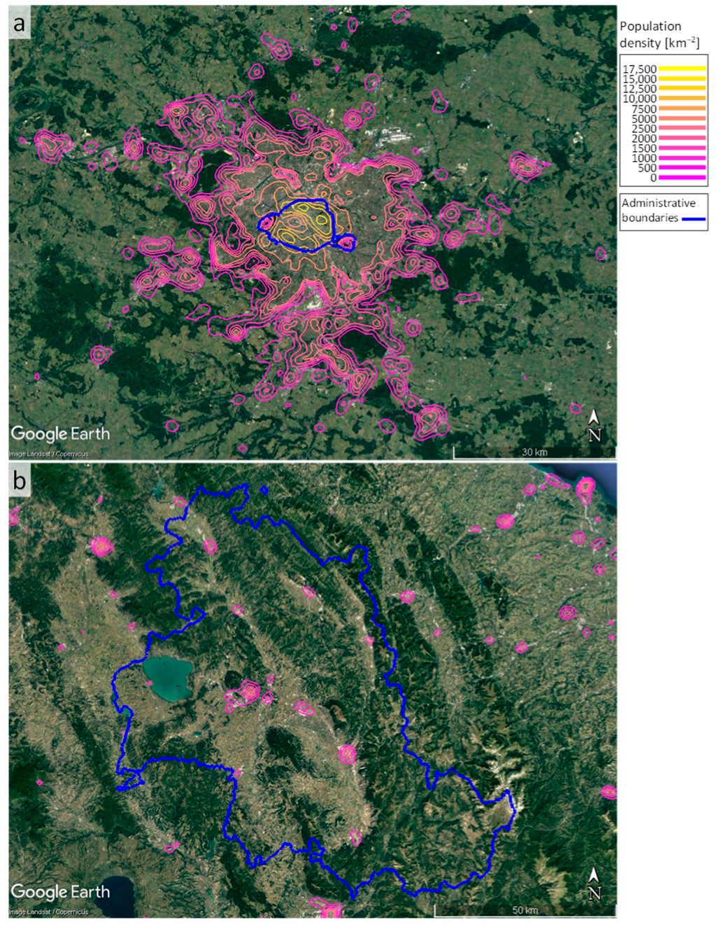
Additionally, it is necessary to clearly identify the spatial boundaries of the urban areas. In this regard, administrative boundaries of settlements do not provide reliable information about the actual boundaries of a certain settlement. As can be seen in Figure 2, the administrative boundary of a city can either enclose an area much smaller than the actual highly populated urban area, such as the French national capital, Paris, or an area much larger than the actual, highly populated urban area, such as the Italian regional capital, Perugia. These two cities were selected because they represent extreme examples from the spectrum of possible cities. Paris is a metropolitan region that has grown together from several formerly separate settlements and can undoubtedly be characterised as an urban area. In Perugia, inhabitants are spread irregularly over an urban core and numerous smaller surrounding settlements. For both sample cities, the method presented should be able to identify areas that can actually be characterised as urban and clearly distinguish them from the extra-urban areas in the study area.

For the calculation of the population-density contours, please refer to the methodology section of this paper. The displayed geospatial boundaries of both cities correspond to OSM admin level 6 [17], which is, in these cases, equivalent to NUTS-3 level [18]. Both cases lead to misclassification if the administrative boundaries of GNSS trajectories from the measurement data are used for classifying the driving domain.

1.2. Related Research

This paper proposes a kernel density estimation (KDE) of urban land use to identify potential urban areas (PUA) within a given digital map. Subsequently, road network scaling models are used to distinguish between urban and extra-urban areas for the identified PUA. Therefore, related studies in the literature are discussed within this subsection regarding urban metrics, land use, the spatial extent of urban areas, use cases of kernel density estimation, and the relationship between settlement size and road network characteristics.

1.3. Urban Metrics and Urban Sprawl

Several metrics exist to measure urban forms and the spatial extent of urban areas. Lowry and Lowry compared a total of 18 spatial metrics, including housing density, population density, mean distance to commercial zones, street connectivity and land-use diversity, when distinguishing between neighbourhood types in Salt Lake County, Utah, USA [19]. Fourteen of the investigated metrics proved to be suitable in distinguishing the investigated neighbourhood types classified as pre-suburban, suburban and late-suburban. They also found strong correlations between several metrics, especially between population density and housing density.

Saksena et al. analysed Vietnam’s urban transition by distinguishing between urban core, urban, transitional (i.e., peri-urban) and rural areas from a socio-spatial perspective [20]. Among other metrics, the fraction of households with a mainly agricultural income, the fractions of land under agriculture, forest, and aquaculture, as well as the fraction of houses with modern sanitation were used as characteristics for the classification. This methodology allowed for the quantification of the urban transition over time and a clear identification of the spatial extent of urban areas.

Often, the motivation to utilize urban metrics is to measure urban sprawl, characterising to which degree urban areas with high-population and housing density grow into lower-density areas, which is widely considered as an undesirable development, as it correlates with high land consumption and longer distances between residential areas and commercial centres. Reviewing 114 peer-reviewed articles, Chettry found that no universal definition of urban sprawl exists to date [21]. The study found that several metrics were used in former studies to estimate urban sprawl and the structure of urban areas. While not indicating which of the metrics is best suited to measure urban sprawl or detect urban areas in general, Chettry points out that the use of geographical information systems (GIS) and remote sensing have proven to be invaluable tools in geospatial research. To overcome the lack of available data in developing countries, the study also recommends the use of open-source data in future research.

Lopez investigated urban sprawl in U.S. metropolitan areas between 1970 and 2010 and used a population-density threshold of 3500 people per square mile to distinguish rural or suburban areas from metropolitan areas [22]. The urban metrics used to characterise urban sprawl were from the density balance sprawl index, which is based on the difference between the proportion of the population living in higher-density and lower-density areas. The study relies on data from the U.S. census of the respective years and found that the rate of urban sprawl varies throughout the U.S, thus proving that urban sprawl is neither uniform nor inevitable.

Hennig et al. used weighted urban proliferation (WUP) as a metric to quantify the degree of urban sprawl in Europe at country, state, and 1 km² grid levels [23]. WUP includes the percentage of built-up areas, the dispersion of built-up areas, and the built-up area per inhabitant as indicators of urban sprawl. The study relied on spatial data from the European Copernicus land services and population data from the Eurostat census service. Among various other findings, WUP was proven to effectively identify urban sprawl around urban centres in the 1 km²-grid-level investigation. It excluded more rural regions due to their low percentages of built-up areas as well as urban centres because of their low built-up areas per inhabitant. This indicated that the percentage of built-up areas was a promising parameter with which to identify urban areas for the purpose of this research.

Figure 2. (a) Satellite images with administrative boundaries in blue as mapped in OSM and colour-scaled population density for: (a) the metropolitan region of Paris, map image: Google, Landsat/Copernicus, Data SIO NOA A, U.S. Navy, NGA, GEBCO; and (b) the region of Perugia, map image: Google, Landsat/Copernicus. Source of administrative boundary data: OpenStreetMap contributors [24]. Source of population data: Eurostat [25].

Figure 2. (a) Satellite images with administrative boundaries in blue as mapped in OSM and colour-scaled population density for: (a) the metropolitan region of Paris, map image: Google, Landsat/Copernicus, Data SIO NOA A, U.S. Navy, NGA, GEBCO; and (b) the region of Perugia, map image: Google, Landsat/Copernicus. Source of administrative boundary data: OpenStreetMap contributors [24]. Source of population data: Eurostat [25].

Yue et al. used the ratio between population growth and land-use expansion as a single-dimensional indicator of urban sprawl alongside a multi-dimensional metric consisting of low land-use density, discontinuity of land use, and poor accessibility to estimate urban sprawl for seven cities in the Yangtze River economic belt region in China throughout 1992, 2000 and 2010 [26]. The study found overall good correlation between the single- and multi-dimensional sprawl metrics. Additionally, the variance of urban sprawl between the considered cities could be attributed to multiple influencing factors, including the monocentric or polycentric city type as well as geographical conditions. To calculate the urban metrics, population data from the Chinese census were used alongside with spatial data from the Defense Meteorological Satellite Program satellites.

Dutta and Das used image processing on geographic information system (GIS) data to classify the land-use type of the study area in eastern India into built-up, water body, vegetation, agricultural and temporarily vacant areas to subsequently analyse forms of urban growth and the extent of urban sprawl throughout 1991 to 2016 [27]. The study found that the edge expansion of built-up areas dominated urban growth compared to infill growth and outlying growth, respectively. Built-up areas proved to be a reliable metric of urban forms in this investigation.

1.4. Land-Use Analyses and Urban Density Estimation

To investigate the extent and density of urban areas, land-use categories have been employed in different research works. Jiao used supervised image classification on high resolution satellite images of 28 cities in mainland China throughout 1990 to 2010 to identify the land-use categories built-up, vegetation, water and other lands, defining impervious surface area as urban land in this study [28]. Subsequently, urban land density was calculated for concentric rings around the city centre to measure the spatiotemporal extent of the considered settlements. Jiao found that the relationship between urban land density and distance from the city centre can be described using an inverse S-shape function, displaying high urban density around the city centre that is decreasing outwards.

Li et al. used kernel density estimation to identify aggregation of different urban elements, namely population density, road density, business point-of-interest density, floor area ratio and built-up density from various data sources, including classified satellite images and OSM for the city of Wuhan, China [29]. All urban elements showed an inverse S-shape relationship with the distance from the city centre, with built-up density being the least aggregated urban element. With regard to the focus of the investigation by Li et al., high aggregation is desirable to identify the spatial distribution of urban density within a given city. However, built-up density, as a lesser-aggregated parameter, promises to reliably identify urban settlement boundaries for the purpose of this paper.

Goldblatt et al. used supervised classification on satellite images of urban rim regions to distinguish built-up (BU) and non-built-up (NBU) cells of a 30 m × 30 m grid [30]. They defined a population-density threshold of 40 people per grid cell to identify highly dense urban areas in India. Subsequently, images from the neighbouring grid cells were sampled to manually label these as BU if more than 50% of the cell area was covered by human-made surfaces, and as NBU otherwise, thereby creating ground truth data for the study. After training, the employed random forest classifier reliably distinguished BU from NBU cells. The identified patches of urban land use showed good agreement with population-density data and subjective perception of urban areas in satellite imagery.

Tabassum et al. similarly used maximum likelihood classification to distinguish between five land-use types, namely, agricultural, vegetation, waterbody, settlement/built-up area and bare land on a 30 m × 30 m grid [31]. Subsequently, the obtained land-use data were used to investigate changes in land use over time and the relationship between land-use types and surface temperatures for the study area in Bangladesh. The study found that the observed increase in land-surface temperature was strongly related to the increase in built-up and bare land and the decrease in vegetated land.

Cianfarani et al. used data from the Oklahoma County Assessor Geodatabase (GDB), the Regrid OKC Urban Core GDB, to identify urban vacant land in the metropolitan area of Oklahoma, USA [32]. Throughout the study it became clear that several land-use types, including steep parcels, upland forests, agricultural land, railroads, highways, and parks, needed be subtracted from the non-built-up areas to identify areas that were truly vacant for urban development. These land-use types were identified manually using satellite and street view images. The study found that the need for new housing units in the city could be met entirely by the considered developable vacant land in the urban core of Oklahoma.

1.5. Relationship between Road Network and City Size

The abovementioned studies in the literature focus on the spatial and socio-economic characteristics of settlements and the resulting urban classifications. However, the relationship between road network characteristics and urban classification is also of importance for the objective of this paper.

Using a biologically inspired approach, Samaniego and Moses formulated two models for scaling a city’s road capacity with increasing city sizes, with one assuming a fully monocentric city and the other addressing polycentric cities [33]. The polycentric model was found to successfully predict road capacity for U.S. cities. However, neither the monocentric nor the polycentric model accurately predicted travel demand within the city, which was found to be best described by a mixture of the two models. Population size and city area served as predictors, while the road capacity was described by means of lane miles, i.e., the total length of the road network, taking into account the number of lanes.

Taillanter and Barthelemy found two thresholds with respect to the number of city commuters for the qualitative characteristics of the urban road network [34]. Above approximately 10⁴ commuters indicated an urban freeway in U.S. urban areas, while a ring road was identified as having more than 10⁵ commuters. A one-dimensional cost–benefit framework was successfully proposed to explain the observations.

1.6. Summary of the Related Research

A clear distinction between urban and non-urban areas is not commonly accepted, as multiple settlement hierarchies exist. Regarding the focus of this paper, the goal is to distinguish between the urban and extra-urban driving domain from a road infrastructure perspective. Therefore, the necessary settlement hierarchy can be simplified to two levels, namely, the presence and absence of a settlement of a certain spatial extent and, hence, the road network characteristics.

The abovementioned literature review also reveals that several methodologies and metrics exist to describe urban forms and urban extents. However, most studies focus on a single area or multiple specific metropolitan areas to identify land-use types within the spatial boundaries of the study area. Only the methodology presented by Hennig et al. [23] was applied to a broader study area spanning multiple countries of Europe, without predefining areas as metropolitan. The study revealed built-up areas to be a reliable indicator of urban areas, independent of the degree of urban sprawl.

The abovementioned research on urban road network characteristics relies on a priori definitions of urban areas or cities. However, the monocentric and polycentric scaling model introduced by Samaniego and Moses [33] is suitable for distinguishing between two classes of urban areas, namely, monocentric and polycentric settlements.

As can be seen in most of the imagery of papers discussed above, urban areas are not ideally agglomerated patches, but may be spread out with non-urban gaps in between. With respect to the aim of this paper, it is not desirable to identify these gaps as non-urban, but instead to classify broader areas. The research of Jiao [28] and Li et al. [29] showed that kernel density estimation is an effective way to spatially smooth urban metrics.

Finally, it needs to be pointed out that most studies either rely on governmental census data as a direct data source, or utilize remote sensing methods, which rely on aerial or satellite images as an indirect data source that is processed with supervised image classification. While accurate census data are not available across all countries, aerial images may differ significantly across climate zones and architectural styles, limiting the universal applicability of a locally trained classification algorithm. Additionally, the identification of road infrastructure features, such as intersections, traffic lights, number of lanes, etc., cannot be derived from remote sensing data. Since the aim of this study is to classify driving domains based on a single readily available data source, open-source maps, namely, OSM, are used as the primary data source. Spatial population census data were used for validation throughout the process but this is not required to apply the classification method to other study areas.

2. Methodology

2.1. Overview

As expressed in the literature review section of this paper, the settlement hierarchy was simplified to distinguish between urban and extra-urban areas. OSM were used as a source of geospatial data for land-use types. The land-use types in OSM are re-categorised into two broader types: urban and non-urban land use. A spatial grid of 200 m × 200 m cell size was used to classify the grid cells into these categories depending on whether or not urban land use occurred within the grid cell: if urban land use occurred, the cell was classified as urban, otherwise the cell was classified as non-urban. Subsequently, KDE was used to spatially smooth the occurrence of urban cells in order to identify broader agglomerations of otherwise spatially separated urban patches. The KDE results were used to generate a map with urban land-use density (ULUD) values varying between 0 (no urban land use) and 1 (only urban land use). As can be seen in the respective section, an ULUD threshold of 0.5 shows good correlation with population-density contours. Therefore, all areas from the gridded map with ULUD above the threshold were considered as potential urban areas (PUA). To distinguish between urban and extra-urban for the PUA, road network capacity ($C_{RN}$) was introduced as another metric. This metric was calculated from vector graph-based road network data, which are also available in OSM. Only contiguous urban patches with a $C_{RN}$ above a certain threshold were considered to belong to the urban driving domain. This threshold was deducted by analysing the relationship between $C_{RN}$ and transport demand $D_T$ for all the identified PUAs. The overall methodology is visualized in Figure 3. The most important steps are explained in detail in the following subchapters.

2.2. Urban Land-Use Categories in OSM

OpenStreetMap is a free map created by volunteers and is available under the Open Data Commons Open Database license. The map includes various geospatial information, including street networks, points of interest and land-use categories. The density of the map data varies across regions, countries and continents and is continuously growing [24].

The information in OSM can be viewed directly on https://www.openstreetmap.org/ (accessed on 5 July 2023) or other websites focussing on different information levels of OSM, e.g., https://osmlanduse.org/ (accessed on 30 March 2024) for land-use visualization or https://osm-boundaries.com/ (accessed on 12 November 2023) for administrative boundaries. Alternatively, OSM data can be retrieved through the Overpass API, either using the web-based data mining tool Overpass turbo (https://overpass-turbo.eu/, accessed on 30 March 2024) or with dedicated libraries for several programming languages. In this study, the Python package OSMnx (available at https://github.com/gboeing/osmnx, accessed on 5 July 2023) was used to download and pre-process OSM data. Boeing provides an introduction and overview of OSMnx [35].

Land use is classified in a total of 40 types/values in OSM under the key landuse. Additionally, the key leisure is also considered as it holds, among others, the key parks, which are commonly found within metropolitan areas. As the aim of this paper is to distinguish between urban and extra-urban areas, the OSM land-use types were categorized accordingly, as presented in

Table 1. Types of land use in OSM [36] and their assignment to the superordinate classes urban/non-urban.

S. No.	Key	Value	Comment	Classification
1	landuse	commercial	-	urban
2		construction	-
3		education	-
4		fairground	-
5		industrial	-
6		residential	-
7		retail	-
8		institutional	-
9		cemetery	old cemeteries are often found inside urban areas
10		garages	-
11		port	high spatial share of port cities is part of the port area
12	leisure	park	many metropolitan areas include parks for leisure
13	landuse	aquaculture	-	non-urban
14		allotments	allotments are mainly placed at the rim of urban areas
15		farmland	-
16		farmyard	-
17		paddy	-
18		animal_keeping	-
19		flowerbed	-
20		forest	-
21		greenhouse_horticulture	built-up land but in extra-urban areas
22		meadow	-
23		orchard	-
24		plant_nursery	-
25		vineyard	-
26		basin	-
27		reservoir	-
28		salt_pond	-
29		brownfield	-
30		conservation	-
31		depot	-
32		grass	-
33		greenfield	-
34		landfill	-
35		military	-
36		quarry	-
37		railway	-
38		recreation_ground	-
39		religious	-
40		village_green	-
41		winter_sports	-

. It needs to be pointed out that the original OSM land-use types are classified by voluntary users; hence, the classification can be influenced by the subjective perception of single OSM creators. The list presented in Table 1 is based on the recommendations from the OSM Wiki page. Future users of the presented method are advised to review the current OSM Wiki recommendations and to update the classification of land-use labels, if necessary [36].

All used OSM data were retrieved from OpenStreetMap contributors [24].

2.3. Kernel Density Estimation of Urban Land Use and Population Density

Even in high-density urban areas, non-urban spatial patches occur frequently, making it difficult to define an entire agglomerated area as an urban driving domain. Therefore, KDE is used to spatially smooth the occurrences of urban land use.

The general formulation of the KDE algorithm is

$$f\left(x\right)=\frac{1}{nh}\cdot {\sum }_{i-1}^{n}K\left(\frac{x-x_i}{h}\right)$$

(1)

with

$f\left(x\right)$: the estimated spatial density at the estimation point,

$x$: the estimation point,

$x_i$: the spatial location of each occurrence,

$x-x_i$: the distance between estimation point and occurrence location,

$n$: the total number of occurrences,

$h$: the kernel bandwidth and

$K$: the kernel function.

The kernel function and the bandwidth must be selected. As a smooth density distribution is beneficial for the present use-case, a Gaussian kernel was selected for this study. Generally, the smoothness of the density distribution increases with increasing bandwidth, while the spatial accuracy decreases. With respect to the scope of this paper, a very low bandwidth would lead to insufficient smoothing, resulting in urban areas perforated with non-urban areas. On the other hand, a very high bandwidth would lead to imprecise boundaries of the identified urban areas. A bandwidth of 1000 m was proven to be a sufficient compromise in this study.

From the previously defined land-use classification, information about the location and size of urban surfaces was known. However, KDE requires input data in the form of occurrences across a certain metric, which was the spatial location in this case. Therefore, it was necessary to discretize the spatial dimensions of the map, leading to a grid. In this study, a grid cell size of 200 m × 200 m is used. Each grid cell is labelled as urban or non-urban, depending on whether or not the urban land use according to Table 1 occurs within the cell. Subsequently, the spatial locations of all urban cells were used as inputs for the KDE.

To validate the general functionality of the urban land-use density approach, population density was used as an alternative metric to identify urban areas. In the 2021 EU population and housing census, population density was not only measured on various administrative levels, but also in a geospatial 1 km × 1 km grid [37]. The data are available for download from Eurostat [25]. The data format of this dataset is given as population-density values for each spatial grid cell. For the purpose of this paper, the data are smoothed with KDE, using a Gaussian kernel, a bandwidth of 1000 m and the mapped population density as the respective kernel weight.

The decision to use a 200 m × 200 m grid for land-use classification in combination with the 1000 m KDE bandwidth resulted from the following considerations. A finer classification grid would increase the numerical calculation effort drastically while theoretically providing more accurate spatial distinction between areas of urban and non-urban land use. However, the final aim of the method is to identify settlements as an entity, not distributions of land use within a settlement. A finer classification grid alongside a finer KDE bandwidth would result in loosely connected patches of urban land use and fail to reliably identify entire urban areas. On the other hand, further increasing the grid size and bandwidth would fail to distinguish between cities and smaller villages that are separated from the urban area by kilometres. Additionally, the KDE bandwidth of 1000 m provides a spatial resolution of land use comparable to the grid size of the EU census data. Census data on a finer grid are not available for the EU.

Applying KDE to the land-use grid and population grid resulted in contour lines of constant urban land-use density (ULUD) and constant population density, respectively. As discussed in detail in the results section of this paper, areas within the ULUD contour of 0.5 and higher are considered as potential urban areas (PUA).

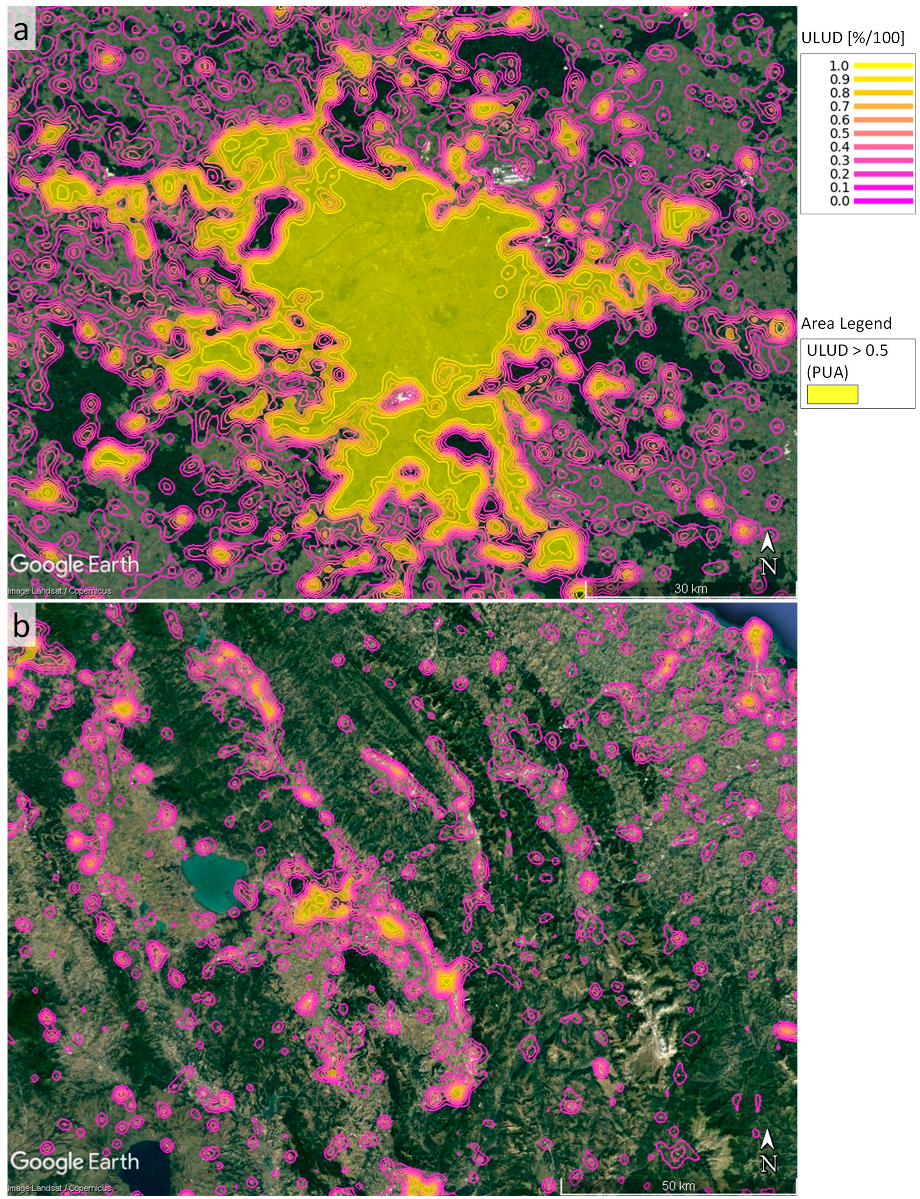
Using the methods described above, Figure 4 and Figure 5 show the results of the spatial KDE analyses for the metropolitan region of Paris and the region of Perugia, respectively. Figure 4 displays the calculated ULUD contours, ranging between 0 and 1, as well as the areas with an ULUD greater than the considered threshold of 0.5. For Paris, these areas spread far over the previously discussed administrative boundary and generally share a similar geometry with the formerly discussed population-density contours. However, while the ULUD reaches the maximum value of 1 throughout the entire urban core of Paris, the population density shows variances within the urban core. This leads to the conclusion that the definition of ULUD in this paper is suitable for detecting the boundary of an urban area, while it is unsuitable for distinguishing between different areas within the urban core of a city. Population density, on the other hand, is suitable for the latter purpose, as it can identify different centres within the urban core of Paris.

At first glance, this seems to contradict the findings of previous research, where KDE of land-use classes was successfully used to identify urban centres within polycentric settlements [28,29]. Closer inspection leads to the following explanation: the grid cells employed in this research were labelled as urban or non-urban discretely based on the presence of urban land use in the respective cell. It can be assumed that using the area share of urban land use of each cell as the kernel weight for KDE led to more nuanced ULUD values within urban areas.

As can be seen in Figure 4b, the identified areas with high ULUD cover only the core and highly populated area within the administrative boundaries of Perugia. Both for Paris and Perugia, ULUD provides results for the distribution of potential urban areas even in areas far from the respective urban core, where population density is too low to provide any further insight.

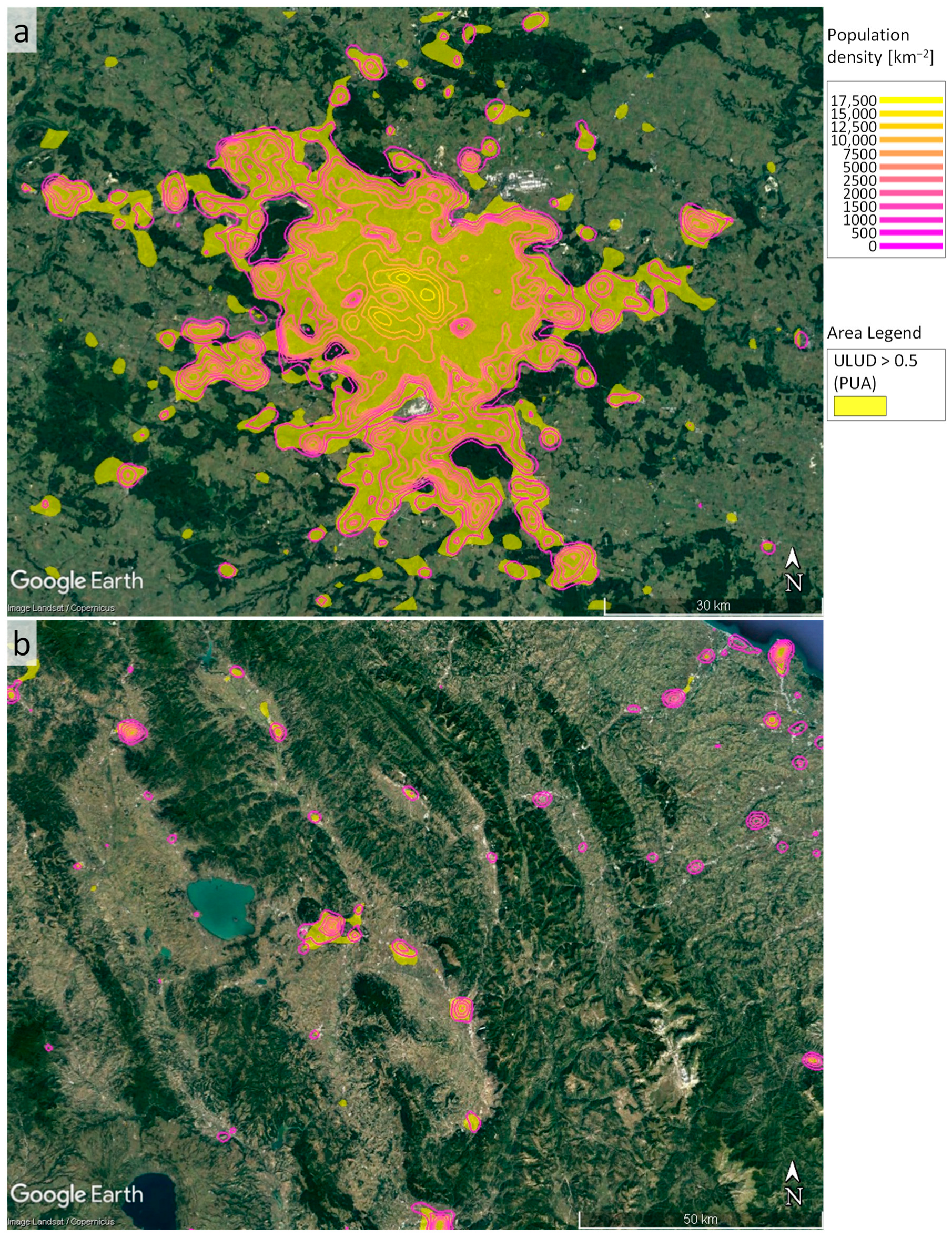
To investigate the relationship between ULUD and population density further, Figure 5 shows areas with ULUD > 0.5 in direct comparison to population-density contours for the two study areas. As can be seen, the ULUD threshold of 0.5 shows good correlation with the population-density contour of Paris at 500 km⁻². The same relationship can be seen in the analysis of Perugia. Therefore, the proposed urban land-use density and the population density can serve as redundant indicators of potential urban areas. The previously discussed figures displayed the successful identification of areas with a high ULUD as PUA. To further filter the identified areas, a method is required to distinguish between urban areas and extra-urban settlements.

2.4. Road Network Scaling Model

Biologically inspired models for the scaling of road networks were proposed by Samaniego and Moses [33]. Their basic assumption is that the transport capacity of a city’s road network meets the transport demand of the city. Road network capacity $C_{RN}$ is calculated by means of lane kilometres with the equation:

$$C_{RN}={\sum }_{i=1}^m{l}_{R,i}\cdot n_{L,i} ,$$

(2)

with

$C_{RN}$: the road network capacity of a certain PUA,

$l_{R,i}$: the length of each road within the PUA,

$n_{L,i}$: the number of lanes of each road within the PUA,

$m$: the total number of roads within the PUA.

According to the metabolic scaling theory formulated by Samaniego and Moses, this capacity is proportional to the transport demand, which is distinguished between the assumptions of monocentric growth (Equation (3)) and polycentric growth (Equation (4)) [33]:

$$C_{RN,mono}\propto D_{T,mono}=N\cdot \sqrt{A} ,$$

(3)

$$C_{RN,poly}\propto D_{T, poly}=\sqrt{N\cdot A} ,$$

(4)

with

$C_{RN,mono}$: the road network capacity of a certain PUA according to the monocentric model,

$D_{T,mono}$: the transport demand of a certain PUA according to the monocentric model,

$C_{RN,poly}$: the road network capacity of a certain PUA according to the polycentric model,

$D_{T,poly}$: the transport demand of a certain PUA according to the polycentric model,

$N$: the number of inhabitants of the PUA,

$A$: the area of the PUA.

The U.S. cities analysed by Samaniego and Moses with this approach ranged between $5\cdot {10}^3$ and $3.5\cdot {10}^7$ inhabitants and showed good agreement for the polycentric model across all city sizes [33]. The PUAs analysed in this paper show a significantly broader population spectrum, reaching down to as low as 100 inhabitants. As can be seen in the log–log diagram in Figure 6a, the polycentric model shows generally good agreement between the observed and predicted $C_{RN}$ (as indicated by the logarithmic slope $b_{log}=1.08$ being close to $b_{log,ideal}=1.0$). However, closer inspection reveals that the model fit is more accurate for a PUA with a higher road network capacity $C_{RN}$.

Therefore, a road network capacity threshold $c_{th}$ was introduced, above which the polycentric scaling model is applied, and below which the monocentric scaling model is used. Figure 6b displays two quality metrics of the model for a varying threshold $c_{th}:$ The deviation between the logarithmic slope $b_{log}$ and the ideal logarithmic slope $b_{log,ideal}=1.00$ is shown in the top half for the monocentric, polycentric and combined models, while the coefficient of determination $R^2$ is displayed in the bottom half for the combined model as well as the purely monocentric and purely polycentric model. As can be seen, a threshold value of $c_{th}={10}^{2.30} \mathrm{k}\mathrm{m}=198 \mathrm{k}\mathrm{m}$ provides the best model agreement regarding $b_{log}$ and $R^2$ for the combined model. However, the monocentric scaling model shows poor performance across all threshold values and the increase in the combined model accuracy towards the optimum resulted mainly from the polycentric model gaining quality of fit.

Both the monocentric and polycentric models consider transport demand as a function of population and urban area. However, for small settlements it can be assumed that the increase in the length of the road network is mainly driven by accessibility rather than population growth. Therefore, the following new scaling model for small settlements was introduced:

$$C_{RN,SS}\propto D_{T,SS}=\sqrt{A}$$

(5)

with

$C_{RN,SS}$: the road network capacity of a certain PUA according to the small settlement model,

$D_{T,SS}$: the transport demand of a certain PUA according to the small settlement model,

$A$: the area of the PUA.

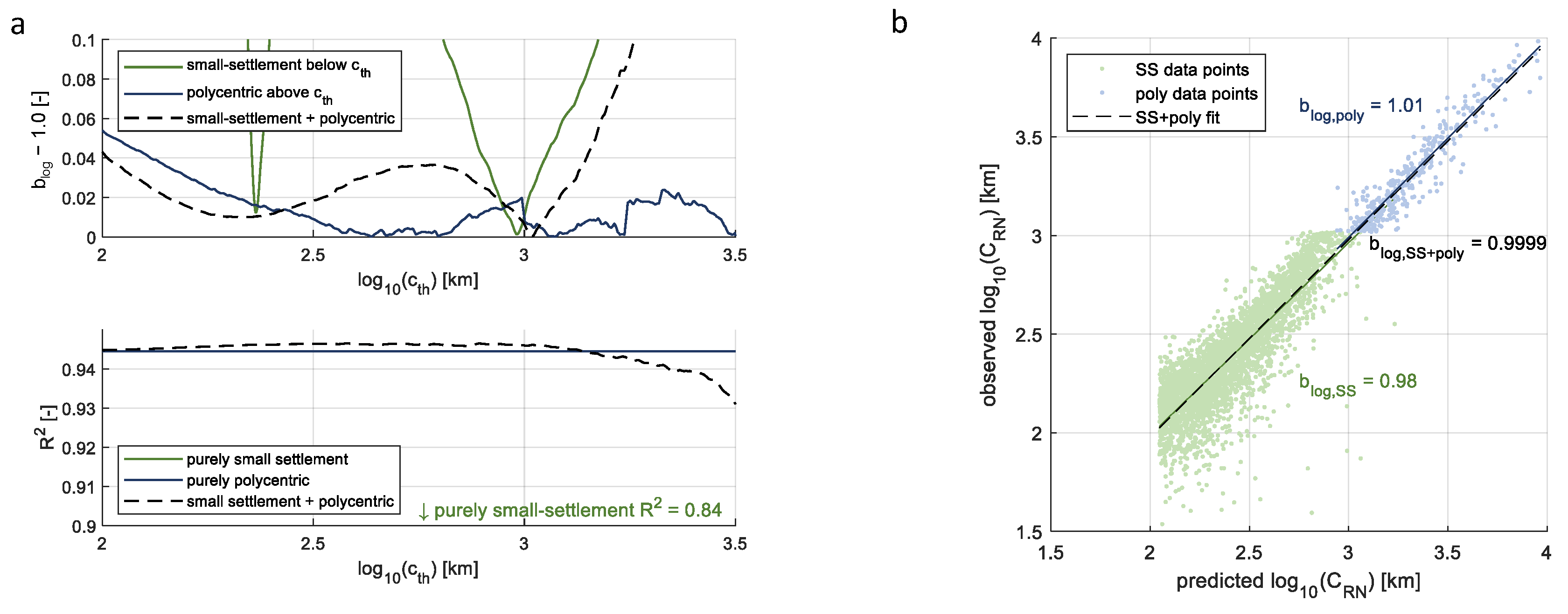
Again, the threshold $c_{th}$ is varied for the combined polycentric scaling model (Equation (4)) and small settlement scaling model (Equation (5)). Figure 7a shows the resulting deviations between $b_{log}$ and $b_{log,ideal}$ for both separate models and the combined model as well as the coefficients of determination $R^2$ for the combined model as well as for the pure polycentric and pure small settlements model. As can be seen, the best model agreement is achieved for a threshold of $c_{th}={10}^{3.02} \mathrm{k}\mathrm{m}=1042 \mathrm{k}\mathrm{m}$. The log–log diagram for the combined model with this threshold value is displayed in Figure 7b. This threshold is used in the following to distinguish between urban and extra-urban areas for all PUAs.

3. Results and Discussion

The previously discussed classification methodology is used to first identify PUA in the European Union based on OSM urban land-use data and to subsequently distinguish the PUA into urban and extra-urban areas. To continue the previous examples, Figure 8 illustrates the final classification of the previously identified PUA. As can be seen, the classification successfully identifies the urban core of Paris and the city of Perugia as urban, while the surrounding PUAs are labelled as extra-urban.

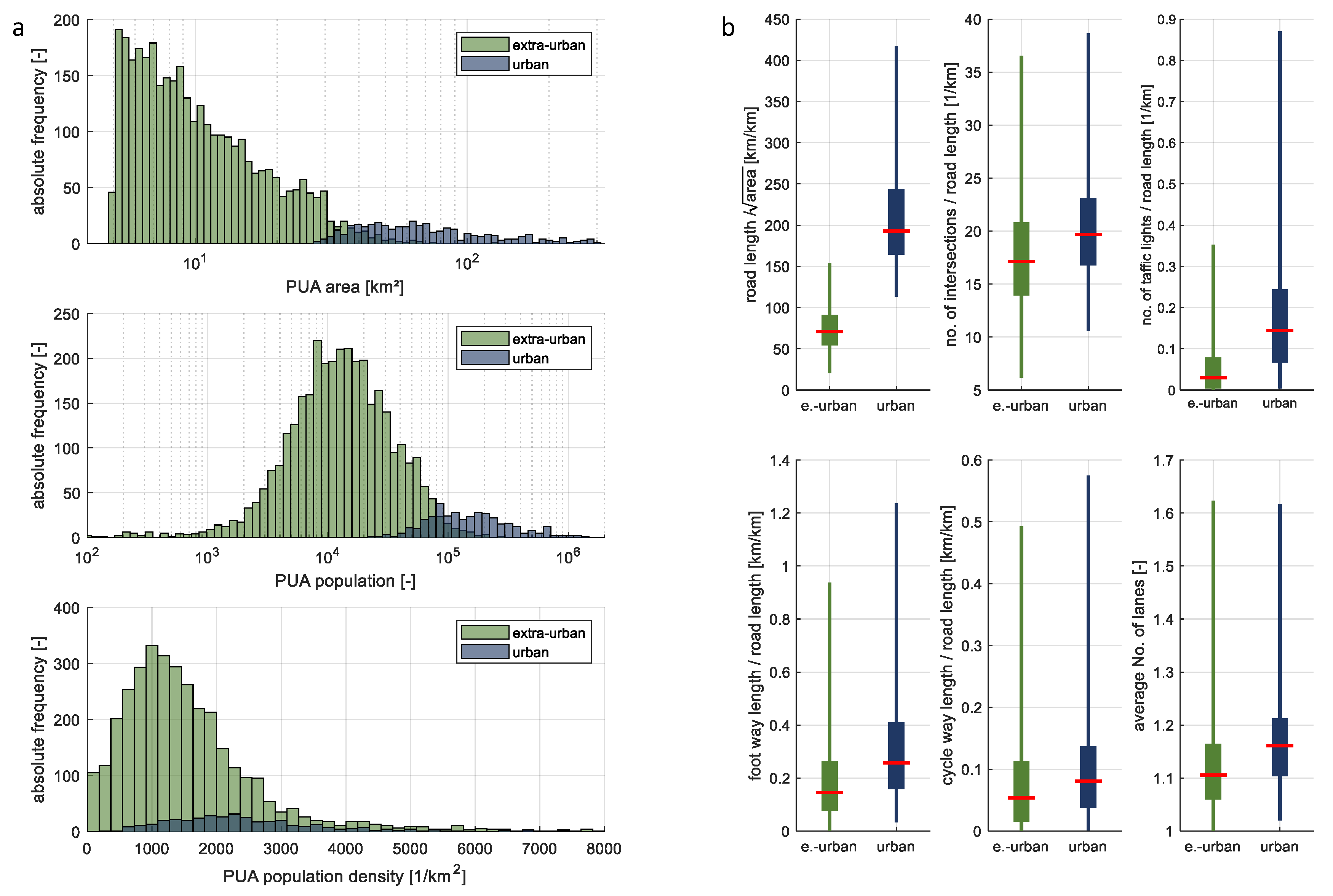
Figure 9a shows frequency distributions of area, total population, and average population density for both urban and extra-urban settlements. As can be seen, there is no threshold for either area or total population that clearly distinguishes the two classes. Instead, there is a smooth transition ranging from $27 \mathrm{k}{\mathrm{m}}^2$ to $70 \mathrm{k}{\mathrm{m}}^2$ and $38\cdot {10}^3$ to $220\cdot {10}^3$ inhabitants. This allows for the interpretation that urban areas are to be characterised by the combination of spatial extent and population. Additionally, it becomes apparent that average population density is not a suitable criterion with which to distinguish between urban and extra-urban settlements, as the value ranges for both classes overlap significantly. However, maximum population density, which might vary between the two settlement classes, was been accessed in this study.

Subsequently, both urban and extra-urban settlements were analysed regarding the distribution of the selected road infrastructure features that are available in OSM. The boxplots in Figure 9b indicate the statistical distributions by means of the 1st, 25th, 50th, 75th and 99th percentiles. The clearest distinction between the two settlement classes is to be seen in the quotient of road length and square root of area, which must be attributed to the fact that road length and area were used as metrics for the classification. The other parameters show considerable overlap. While this indicates that these metrics alone are not suitable for urban classification, a clear trend can still be observed: urban settlements have a higher density of road junctions, traffic lights, foot ways and cycle ways than extra-urban settlements. Therefore, interaction scenarios between the measurement vehicle and these infrastructure elements, as well as between other road users (namely, pedestrians and cyclists), will be more frequent in these areas. In addition, urban settlements have a higher proportion of multi-lane roads, resulting in a higher average number of lanes than in extra-urban settlements.

4. Summary and Conclusions

Correct driving domain classification is crucial when analysing fleet measurement data for the development of automated driving functions. While driving in the highway domain can be classified via map-matching and mapped road types, distinguishing between urban and extra-urban driving domains requires a geospatial approach. Administrative boundaries do not distinguish reliably between urban and extra-urban areas for two reasons: First, the administrative boundary of a settlement does not necessarily coincide with its actual boundary. Second, settlement hierarchy is not globally standardized. The literature review of this paper revealed population density as a promising metric with which to identify potential urban areas. With the 2021 EU population and housing census, high-resolution geospatial population-density data have become available for Europe. However, these data are not available on a global scale.

Therefore, this paper proposes urban land-use density (ULUD) as a reliable metric with which to identify contiguous potential urban areas. ULUD is calculated using kernel density estimation on the geospatial data of land-use categories mapped and labelled in OSM. The ULUD approach shows similarities to population density as an alternative urban metric. The results indicate that ULUD and population density are redundant metrics for identifying potential urban areas, where an ULUD level of 0.5 correlates well with a population-density level of 500 km⁻². Hence, ULUD can be used for the identification of potential urban areas where no sufficient population-density data are available, given the availability of reliable land-use classification maps. Other data sources commonly used in geospatial analysis, such as remote-sensing data and night light images, are to be used for further validation of the ULUD metric in future research. This is particularly important if the method is to be transferred to other study areas where no census data are available.

Urban road network scaling models were introduced in this paper to distinguish between urban and extra-urban classes for the identified potential urban areas. While an existing approach for polycentric settlements showed good performance for larger PUAs, the introduction of a novel road network scaling model was necessary for small settlements. Areas where the road network capacity could be modelled using the polycentric scaling approach were classified as urban, while areas where the road network capacity could be modelled using the small settlement scaling approach were classified as extra-urban. While the development and validation of the described classification methodology required spatial population data, the application of the methodology only requires urban land-use data and road infrastructure data, which are both available from OSM. This enables urban classification even in regions where no spatial population data are available. Instead of OSM, other data sources, like remote sensing, are also possible enablers of urban classification.

Subsequently, selected road infrastructure features were analysed for the classified urban and extra-urban areas, revealing that there is no clear distinction between the two settlement classes regarding these metrics. However, clear trends are visible, indicating that traffic lights, intersections, foot ways, cycle ways and multi-lane roads occur more frequently in urban areas than in extra-urban settlements.

Based on the presented approach, further research is needed to analyse the characteristics of urban and extra-urban driving domains with regard to traffic density, vehicle trip length, and driving behaviour, among other parameters. Lastly, the presented methodology can be used in other geospatial analyses, e.g., to preliminarily identify the relevant spatial extent of the settlement under investigation.

References

1. SAE International/ISO. Surface Vehicle Recommended Practice: Taxonomy and Definitions for Terms Related to Driving Automation Systems for On-Road Motor Vehicles, 2021-04; SAE. (J3016). 2021. Available online: https://www.researchgate.net/publication/355980391_SURFACE_VEHICLE_RECOMMENDED_PRACTICE_R_Taxonomy_and_Definitions_for_Terms_Related_to_Driving_Automation_Systems_for_On-Road_Motor_Vehicles (accessed on 26 November 2023).
2. PAS 1883:2020; Operational Design Domain (ODD) Taxonomy for an Automated Driving System (ADS): Specification. The British Standards Institution, BSI Standards Limited: London, UK, 2020.
3. ISO 34503:2023; Road Vehicles—Test Scenarios for Automated Driving Systems—Specification for Operational Design Domain. International Organization for Standardization: Geneva, Switzerland, 2023.
4. Ye, X.; Wang, X. Operational design domain of automated vehicles at freeway entrance terminals. Accid. Anal. Prev. 2022. [Google Scholar] [CrossRef]
5. Vreeswijk, J.; Wijbenga, A.; Schindler, J. Cooperative Automated Driving for managing Transition Areas and the Operational Design Domain (ODD). In Proceedings of the 8th Transport Research Arena TRA, Rethinking Transport. TRA2020, Helsinki, Finland, 27–30 April 2020. [Google Scholar]
6. Bernstein, D.; Kornhauser, D. An Introduction to Map Matching for Personal Navigation Assistants; New Jersey Institute of Technology: Newark, NJ, USA, 1996. [Google Scholar]
7. Quddus, M.A.; Ochieng, W.Y.; Zhao, L.; Noland, R.B. A general map matching algorithm for transport telematics applications. GPS Solut. 2003, 7, 157–167. [Google Scholar] [CrossRef]
8. Yang, H.; Cheng, S.; Jiang, H.; An, S. An Enhanced Weight-based Topological Map Matching Algorithm for Intricate Urban Road Network. Procedia—Soc. Behav. Sci. 2013, 96, 1670–1678. [Google Scholar] [CrossRef]
9. Lou, Y.; Zhang, C.; Zheng, Y.; Xie, X.; Wang, W.; Huang, Y. Map-matching for low-sampling-rate GPS trajectories. In Proceedings of the 17th ACM SIGSPATIAL International Conference on Advances in Geographic Information Systems; Association for Computing Machinery: New York, NY, USA, 2009. [Google Scholar] [CrossRef]
10. Uni Münster. Definitionen: Stadtbegriff. Available online: https://www.uni-muenster.de/Staedtegeschichte/portal/einfuehrung/Definitionen.html (accessed on 9 November 2023).
11. Bhagat, R.B. Rural-urban classification and municipal governance in India. Singap. J. Trop. Geogr. 2005, 26, 61–73. [Google Scholar] [CrossRef]
12. Bundesinstitut für Bau-, Stadt- und Raumforschung. Raumbeobachtung: Stadt- und Gemeindetypen in Deutschland. Available online: https://www.bbsr.bund.de/BBSR/DE/forschung/raumbeobachtung/Raumabgrenzungen/deutschland/gemeinden/StadtGemeindetyp/StadtGemeindetyp.html (accessed on 9 November 2023).
13. Geography Revision. Hierarchy of Settlements. Available online: https://geography-revision.co.uk/a-level/human/hierarchy-of-settlements/#Introduction_to_hierarchy_of_settlements (accessed on 9 November 2023).
14. Tarrant, J.R. A Note concerning the Definition of Groups of Settlements for a Central Place Hierarchy. Econ. Geogr. 1968, 44, 144–151. [Google Scholar] [CrossRef]
15. Lynch, K.A. What Is the Form of a City, and How Is It Made? In Urban Ecology: An International Perspective on the Interaction between Humans and Nature; Marzluff, J.M., Shulenberger, E., Endlicher, W., Alberti, M., Bradley, G., Ryan, C., zum Brunnen, C., Simon, U., Eds.; Springer: New York, NY, USA, 2008; pp. 677–690. ISBN 978-0-387-73411-8. [Google Scholar]
16. Müller-Ibold, K. Einführung in die Stadtplanung: Band 1: Definitionen und Bestimmungsfaktoren; W. Kohlhammer: Stuttgart, Germany, 1996; ISBN 978-3-8348-1632-0. [Google Scholar]
17. OpenStreetMap Contributors. Planet Dump. Available online: https://planet.osm.org (accessed on 5 July 2023).
18. Eurostat. NUTS 2021 Classification. Table. 2023. Available online: https://ec.europa.eu/eurostat/documents/345175/629341/NUTS2021.xlsx (accessed on 2 December 2023).
19. Lowry, J.H.; Lowry, M.B. Comparing spatial metrics that quantify urban form. Comput. Environ. Urban Syst. 2014, 44, 59–67. [Google Scholar] [CrossRef]
20. Saksena, S.; Fox, J.; Spencer, J.; Castrence, M.; DiGregorio, M.; Epprecht, M.; Sultana, N.; Finucane, M.; Nguyen, L.; Vien, T.D. Classifying and mapping the urban transition in Vietnam. Appl. Geogr. 2014, 50, 80–89. [Google Scholar] [CrossRef]
21. Chettry, V. A Critical Review of Urban Sprawl Studies. J. Geovisualization Spat. Anal. 2023, 7, 28. [Google Scholar] [CrossRef]
22. Lopez, R. Urban Sprawl in the United States: 1970–2010. Cities Environ. (CATE) 2014, 7. Available online: https://digitalcommons.lmu.edu/cgi/viewcontent.cgi?article=1131&context=cate (accessed on 25 April 2024).
23. Hennig, E.I.; Schwick, C.; Soukup, T.; Orlitová, E.; Kienast, F.; Jaeger, J.A. Multi-scale analysis of urban sprawl in Europe: Towards a European de-sprawling strategy. Land Use Policy 2015, 49, 483–498. [Google Scholar] [CrossRef]
24. OpenStreetMap Wiki Contributors. About OpenStreetMap: OpenStreetMap Wiki. Available online: https://wiki.openstreetmap.org/w/index.php?title=About_OpenStreetMap&oldid=2310396 (accessed on 12 November 2023).
25. Eurostat. Data of the 2021 Population and Housing Census in the EU. GeoPackage (gpkg). 2023. Available online: https://gisco-services.ec.europa.eu/census/2021/Eurostat_Census-GRID_2021_V1-0.zip (accessed on 13 November 2023).
26. Yue, W.; Zhang, L.; Liu, Y. Measuring sprawl in large Chinese cities along the Yangtze River via combined single and multidimensional metrics. Habitat Int. 2016, 57, 43–52. [Google Scholar] [CrossRef]
27. Dutta, I.; Das, A. Application of geo-spatial indices for detection of growth dynamics and forms of expansion in English Bazar Urban Agglomeration, West Bengal. J. Urban Manag. 2019, 8, 288–302. [Google Scholar] [CrossRef]
28. Jiao, L. Urban land density function: A new method to characterize urban expansion. Landsc. Urban Plan. 2015, 139, 26–39. [Google Scholar] [CrossRef]
29. Li, Z.; Jiao, L.; Zhang, B.; Xu, G.; Liu, J. Understanding the pattern and mechanism of spatial concentration of urban land use, population and economic activities: A case study in Wuhan, China. Geo-Spat. Inf. Sci. 2021, 24, 678–694. [Google Scholar] [CrossRef]
30. Goldblatt, R.; You, W.; Hanson, G.; Khandelwal, A. Detecting the Boundaries of Urban Areas in India: A Dataset for Pixel-Based Image Classification in Google Earth Engine. Remote Sens. 2016, 8, 634. [Google Scholar] [CrossRef]
31. Tabassum, A.; Basak, R.; Shao, W.; Haque, M.M.; Chowdhury, T.A.; Dey, H. Exploring the Relationship between Land Use Land Cover and Land Surface Temperature: A Case Study in Bangladesh and the Policy Implications for the Global South. J. Geovisualization Spat. Anal. 2023, 7, 25. [Google Scholar] [CrossRef]
32. Cianfarani, F.; Abdelkarim, M.; Richards, D.; Kedarisetty, R.K. Assessing the Urban Vacant Land Potential for Infill Housing: A Case Study in Oklahoma City, USA. Urban Sci. 2023, 7, 101. [Google Scholar] [CrossRef]
33. Samaniego, H.; Moses, M.E. Cities as organisms: Allometricscalingofurbanroad networks. J. Transp. Land Use 2008, 1, 21–39. [Google Scholar] [CrossRef]
34. Taillanter, E.; Barthelemy, M. Evolution of road infrastructure in large urban areas. Phys. Rev. E 2023, 107, 34304. [Google Scholar] [CrossRef]
35. Boeing, G. OSMnx: A Python package to work with graph-theoretic OpenStreetMap street networks. JOSS 2017, 2, 215. [Google Scholar] [CrossRef]
36. OpenStreetMap Wiki Contributors. DE:Key:landuse: OpenStreetMap Wiki. Available online: https://wiki.openstreetmap.org/w/index.php?title=DE:Key:landuse&oldid=2338525 (accessed on 12 November 2023).
37. Eurostat Press Office. The 2021 Population and Housing Censuses in the EU. Available online: https://ec.europa.eu/eurostat/documents/4031688/14081269/KS-09-21-344-EN-N.pdf/5907978a-011d-52fc-100e-f6a67735d938?t=1641392358489 (accessed on 26 November 2023).
Figure 1. (a) Multiple ODDs within the superordinate driving domain classes urban, extra-urban and highway; and (b) first and second levels of ODD taxonomy according to The British Standards Institution [2].
Urbansci 08 00048 g001
Figure 3. Overview of the driving domain classification methodology proposed in this paper.
Urbansci 08 00048 g003
Figure 4. Satellite image with ULUD contours and area patches with ULUD > 0.5 for: (a) the metropolitan region of Paris, map image: Google, Landsat/Copernicus, Data SIO NOA A, U.S. Navy, NGA, GEBCO; and (b) the region of Perugia, map image: Google, Landsat/Copernicus.
Urbansci 08 00048 g004
Figure 5. Satellite image with population-density contours and area patches with ULUD > 0.5: (a) for the metropolitan region of Paris, map image: Google, Landsat/Copernicus, Data SIO NOA A, U.S. Navy, NGA, GEBCO; and (b): for the region of Perugia, map image: Google, Landsat/Copernicus.
Urbansci 08 00048 g005
Figure 6. (a) log–log diagram of the observed vs. the predicted C R N for the polycentric model; and (b) deviation of b l o g from 1.0 vs. the varied threshold l o g 10 c t h for the monocentric model, polycentric model and combined model. Note: The curves of b l o g 1.0 have been moving average smoothed (n = 10) to enhance visibility.
Urbansci 08 00048 g006
Figure 7. (a) Deviation of b l o g from 1.0 vs. the varied threshold l o g 10 c t h for the small-settlement model, polycentric model, and combined model; and (b) log–log diagram of the observed vs. the predicted C R N for the combined model. Note: The curves of b l o g 1.0 have been smoothed (n = 10) to enhance visibility.
Urbansci 08 00048 g007
Figure 8. Satellite image classification results of the PUAs for: (a) the metropolitan region of Paris; and (b) the region of Perugia. Map Images: Google, Landsat/Copernicus, Data SIO NOA A, U.S. Navy, NGA, GEBCO.
Urbansci 08 00048 g008
Figure 9. (a) Frequency distribution of area, population, and population density for urban and extra-urban settlements; and (b) boxplots of selected road infrastructure features for urban and extra-urban settlements.
Urbansci 08 00048 g009