Article

Contingent Valuation Machine Learning (CVML): A Novel Method for Estimating Citizens’ Willingness to Pay for a Safer and Cleaner Environment

1
Faculty of Development Economics, VNU University of Economics and Business, Vietnam National University, Hanoi 100000, Vietnam
2
School of Civil and Environmental Engineering, University of Ulsan, 93 Daehak-Ro, Nam-Gu, Ulsan 44610, Republic of Korea
3
Vietkaplab, VIETKAP Group, Hanoi 100000, Vietnam
*
Author to whom correspondence should be addressed.
Urban Sci. 2023, 7(3), 84; https://doi.org/10.3390/urbansci7030084
Submission received: 13 July 2023 / Revised: 5 August 2023 / Accepted: 10 August 2023 / Published: 12 August 2023

Abstract

:
This paper introduces an advanced method that integrates contingent valuation and machine learning (CVML) to estimate residents’ demand for reducing or mitigating environmental pollution and climate change. To be precise, CVML is an innovative hybrid machine learning model, and it can leverage a limited amount of survey data for prediction and data enrichment purposes. The model comprises two interconnected modules: Module I, an unsupervised learning algorithm, and Module II, a supervised learning algorithm. Module I is responsible for grouping the data into groups based on common characteristics, thereby grouping the corresponding dependent variable, whereas Module II is in charge of demonstrating the ability to predict and the capacity to appropriately assign new samples to their respective categories based on input attributes. Taking a survey on the topic of air pollution in Hanoi in 2019 as an example, we found that CVML can predict households’ willingness to pay for polluted air mitigation at a high degree of accuracy (i.e., 98%). We found that CVML can help users reduce costs or save resources because it makes use of secondary data that are available on many open data sources. These findings suggest that CVML is a sound and practical method that could be widely applied in a wide range of fields, particularly in environmental economics and sustainability science. In practice, CVML could be used to support decision-makers in improving the financial resources to maintain and/or further support many environmental programs in years to come.

1. Introduction

As climate change and environmental pollution become more prevalent and their effects on human well-being and the environment increase, the private sector plays a growing role in funding environmental projects [1,2]. In practice, measuring the financial contribution of contributors to environmental activities can assist policymakers and/or planners in developing a better plan or stronger environmental policies. Among many approaches adopted to support such activities, contingent valuation (CV) is typically one of the most widely used methods of selection.
Contingent valuation is a survey-based method used for estimating the economic value of non-marketable commodities and services. Because it uses a stated preference approach, consumers are explicitly questioned about their willingness to pay (WTP) for a good or service [3,4]. The CV method has been used to estimate the value of a wide range of goods and services including clean air, clean water, biodiversity, and cultural heritage [5,6,7,8,9]. It has also been used to estimate the costs of environmental damage, such as waste pollution and climate change [3,10,11,12]. Over the last four decades, CV development has been centered on five main directions.
The first is developing better ways to represent goods and services to respondents. In the early days of CV, scholars had trouble getting consumers to reply to questionnaires regarding their WTP for environmental goods and services. But, as time has passed, researchers have improved the manner in which they explain these products and services to respondents, which has increased the number of people who are willing to take part in CV surveys [5]. The second is improving the way WTP is elicited from respondents. Scientists have improved their methods for eliciting WTP from respondents over time. For example, CV surveys used to frequently include an open-ended question that asked respondents to state their maximum WTP. Open-ended questions, on the other hand, may be difficult for responders to answer, resulting in inconsistent responses [13]. The researchers discovered that employing a different question structure, such as one using closed-ended questions that allow respondents to select from a list of specified WTP quantities, is more reliable. The third is dealing with respondents’ strategic behavior [5]. Respondents engage in strategic conduct when they attempt to affect the outcome of a CV survey by answering in a way that they believe will benefit them. Respondents, for example, may overestimate their WTP in order to obtain more money for themselves or their group. To deal with strategic behavior, researchers have developed a number of strategies such as using random payment and providing respondents with enough information about the objectives of their surveys [3]. The fourth is addressing the issue of scope insensitivity [14,15]. This issue refers to cases when respondents’ WTP for a good or service is unaffected by the quantity of the good or service available. Respondents may, for example, be willing to spend the same amount to save a small endangered species as they are to save a large endangered one. Researchers have also found and used a range of strategies to deal with the scope insensitivity. For example, informing respondents about the shortage of the commodities or services in question might lessen the scope insensitivity. The final direction is developing CV models to better estimate WTP values. Take the interval regression model, a typical model used for analyzing payment card data, as an example. This model is a statistical model that is used to estimate the lower and upper bounds of WTP. Interval regression models have been shown to be effective at estimating WTP in CV studies as they can account for uncertainty in the estimates. There have been a number of recent advances in the use of interval regression models to estimate WTP in CV studies in the last two decades. The first advance is the development of Bayesian interval regression models [16]. These models allow for the incorporation of prior information into the estimation of the WTP parameters. This can improve the accuracy of the estimates, especially in cases where the data are limited. Another advance is the development of non-parametric interval regression models [17]. These models do not make any assumptions about the distribution of the WTP parameters. This can be useful in cases where the data are not normally distributed or where the parameters of such models vary across individuals. Although the CV method has been much improved and widely accepted by scientists, agencies, and policymakers in many countries, it remains controversial to some degree [3,5,13,18,19]. CV is currently in development, and efforts to improve its validity and reliability are ongoing [4,13].
Fortunately, machine learning (ML), which is associated with technology and statistics methods, has undergone continuous development over the past few decades. It is now a crucial component of data analysis, and CV can benefit from this advancement. Machine learning algorithms are typically trained on a set of data and then used to make predictions on new data [20]. These algorithms learn from the data by identifying patterns and relationships. For example, a machine learning algorithm could be trained on a dataset of historical weather data to predict the weather in the future. The use of machine learning by users globally has been rapidly increasing in recent years. This growth is being driven by a number of reasons/factors. The first one is the increasing availability of data. Machine learning algorithms require large datasets to train. In the past, these datasets were not available, but they are now available due to the increasing use of the internet and the development of new sensors. The second one refers to the development of more powerful computers. Machine learning algorithms are computationally expensive to train. This is because machine learning algorithms often involve complex mathematical calculations, and these calculations can be very time-consuming and require a lot of processing power. Machine learning algorithms are often trained using an iterative process. The algorithm is trained on the data and then the results are evaluated. Next, the algorithm is retrained using the data and the new results are evaluated. This process is repeated many times until the algorithm converges on a solution. In the past, computers were not powerful enough to train these algorithms, but they are now powerful enough to do so. The third one is the development of new machine learning algorithms. In recent years, many new machine learning algorithms have been developed that are more powerful and efficient than the algorithms that were available in the past [20]. For example, deep learning is a type of machine learning that uses artificial neural networks to learn from data. Deep learning algorithms have been shown to be very effective at a variety of tasks, including image recognition, natural language processing, and speech recognition [21,22]. In addition, ensemble learning is a technique that combines the predictions of multiple machine learning algorithms to improve accuracy [23]. Ensemble learning algorithms have been shown to be very effective at a variety of tasks including classification and regression. The progress that has been made in machine learning over the past few decades is truly remarkable, and machine learning is now a powerful tool that can be used to solve a wide range of problems, and it is likely to play an even greater role in the future.
In this regard, the purpose of the study is to develop and introduce a novel approach that combines contingent valuation and machine learning (CVML) to more accurately estimate households’ willingness to pay for environmental pollution reduction and/or climate change mitigation. This new method is expected to contribute to the literature on non-market valuation in environmental economics and sustainability studies.

2. Contingent Valuation Machine Learning (CVML) Framework

We develop and employ a contingent valuation machine learning (CVML) analytics system in this study (Figure 1).

2.1. Contingent Valuation Procedures

2.1.1. Open-Ended

The open-ended question in the contingent valuation method (CV) is a survey-based technique used to estimate the value of non-market goods and services [3]. In this method, respondents are asked to state the maximum amount of money they would be willing to pay (WTP) for a particular good or service. For example, according to [3], the wording of an open-ended question is: “If the passage of the proposal would cost you some amount of money every year for the foreseeable future, what is the highest amount that you would pay annually and still vote for the program? (WRITE IN THE HIGHEST DOLLAR AMOUNT AT WHICH YOU WOULD STILL VOTE FOR THE PROGRAM)”.
The open-ended format is considered to be the most direct and accurate way to measure WTP, but it can be hard for respondents to answer this type of question. The open-ended format has some advantages. First, this method does not provide respondents with any cues about what the value of the good or service might be. This helps to ensure that respondents’ responses are not influenced by their expectations of what the “correct” answer should be. Second, the method allows respondents to express their WTP in any amount, which can be more accurate than a payment card or dichotomous-choice question, which typically only allows respondents to choose between two or three predetermined amounts. However, the open-ended question also has some disadvantages. First, it can be difficult for respondents to answer this type of question. They may not be familiar with the concept of WTP, or they may not be able to accurately estimate how much they would be willing to pay for a particular good or service. Second, the open-ended format can result in a large number of “don’t know” or “no response” answers. This can make it difficult to obtain a representative sample of respondents and to estimate the mean WTP for a good or service to some degree.

2.1.2. Payment Card

In a CV survey, the payment card question presents respondents with a list of possible WTP amounts, and they are asked to circle the amount that best represents their WTP [3]. For example, according to [3], the wording of a payment card question is: “If the passage of the proposal would cost you some amount of money every year for the foreseeable future, what is the highest amount that you would pay annually and still vote for the program in the Box 1? (CIRCLE THE HIGHEST AMOUNT THAT YOU WOULD STILL VOTE FOR THE PROGRAM)”
Box 1. Payment card question format.
USD 0.1USD 0.5USD 1USD 5USD 10USD 20
USD 30USD 40USD 50USD 75USD 100USD 150
USD 200MORE THAN USD 200
The payment card method has several advantages over the open-ended question, which asks respondents to state their WTP without any guidance. The payment card format provides respondents with a frame of reference, which can help them to make more informed decisions. Additionally, the payment card method is less likely to produce outliers, which are extreme values that can skew the results of a survey. However, the payment card question also has some disadvantages. The list of possible WTP amounts may not be exhaustive, and respondents may not be able to find an amount that accurately reflects their WTP. Additionally, the payment card format can be more time-consuming for respondents to complete than the open-ended CV method.

2.2. Machine Learning Procedures

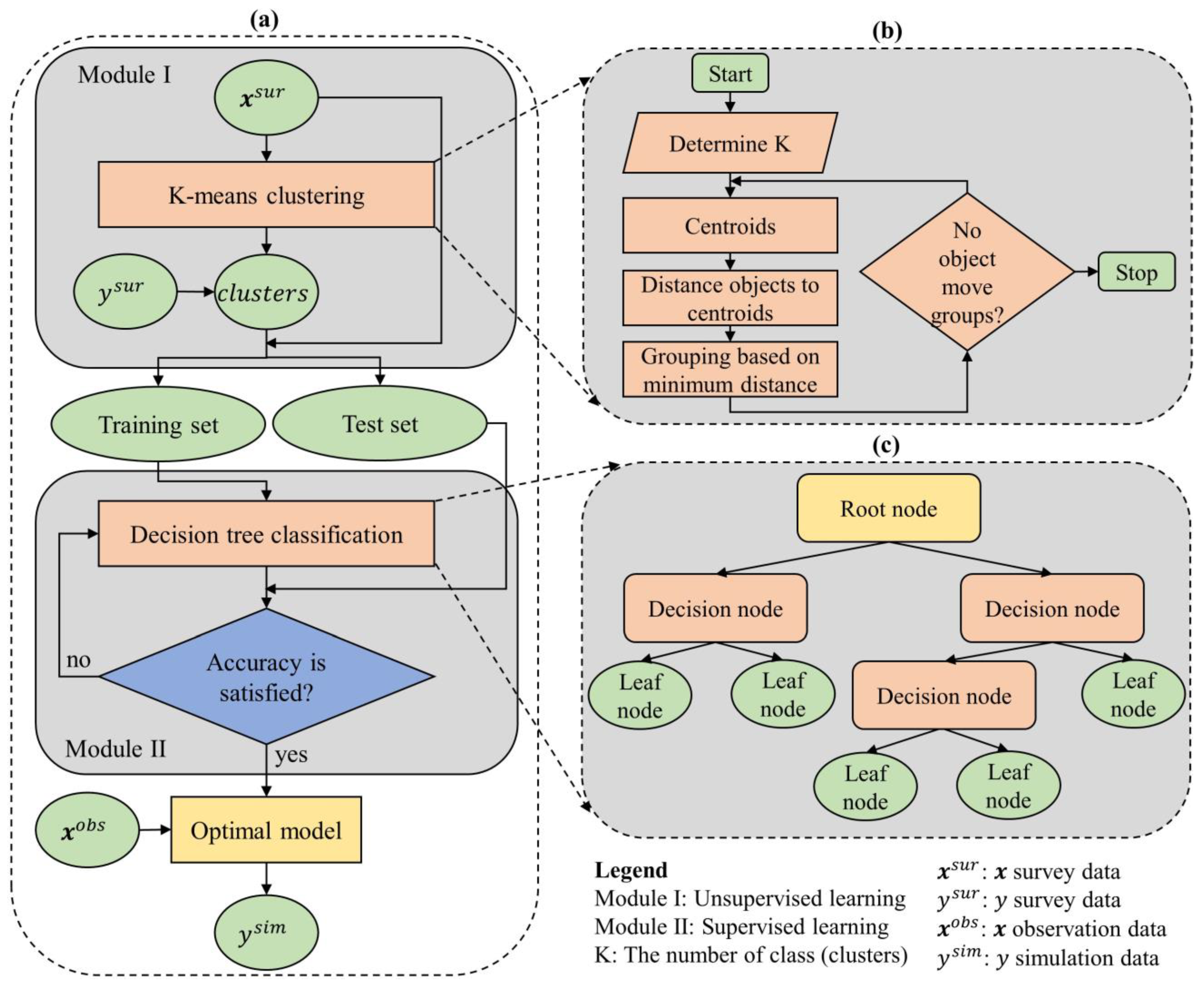
Typically, research endeavors are consistently troubled by issues related to data. The process of collecting data is a challenging task that demands significant investments of time and financial resources. To address this challenge, we propose an innovative hybrid machine learning model that leverages a limited amount of survey data for prediction and data enrichment purposes. Our model comprises two interconnected modules: Module I, an unsupervised learning algorithm, and Module II, a supervised learning algorithm. Module I is responsible for clustering the data ( x sur ) into groups based on common characteristics, thereby grouping the corresponding dependent variable ( y sur ) values as well. The output of Module I comprises the clustered data, which are then fed as input into Module II. In Module II, the output from Module I is utilized to construct a classification prediction model. Once Module II is built and its quality is assessed, it can be employed to predict the dependent variable ( y sim ) using the independent variables ( x obs ) sourced from previous studies or easily collected data. Figure 2a illustrates the comprehensive framework, while Figure 2b,c provide detailed insights into Module I and Module II, respectively.

2.2.1. K-Means Clustering Algorithm (Module I)

K-means clustering is an unsupervised machine learning algorithm widely employed for grouping data points into distinct clusters based on their feature similarity [24]. It operates by iteratively assigning data points to clusters and updating the cluster centroids. To categorize a given dataset into a predetermined number of clusters, the algorithm establishes K centroids, representing the center points of each cluster. It is crucial to position these centroids strategically to achieve an optimal solution globally. Therefore, the most favorable approach is to maximize the distance between centroids by placing them as far apart as possible. Next, every data point is assigned to the cluster whose centroid is closest to it. The algorithm then recalculates k new centroids, which serve as the average positions of all data points within each cluster. The data points are reassigned to the closest new centroid. This process is repeated either for a specific number of iterations or until consecutive iterations yield the same centroids [25]. In the end, the objective of this algorithm is to minimize the total distortion or squared error. Distortion refers to the sum of the distances between data points and their respective cluster centroids [26]. The objective function ( J ) of K-means is given in Equation (1):
J = j = 1 K i = 1 n x i j c j 2
where K is the number of clusters, n is the number of data points, and x i j c j 2 is a Euclidean distance between a data point x i j and centroid c j . Figure 1b shows the algorithmic steps of the K-means clustering.
Step 1: Place K data items into the space to represent initial group centroids.
Step 2: Assign each data item to the group that has the closest centroid to that data item.
Step 3: Calculate the positions of K cluster centroids.
Step 4: Repeat Steps 2 and 3 until the positions of the centroids no longer change.
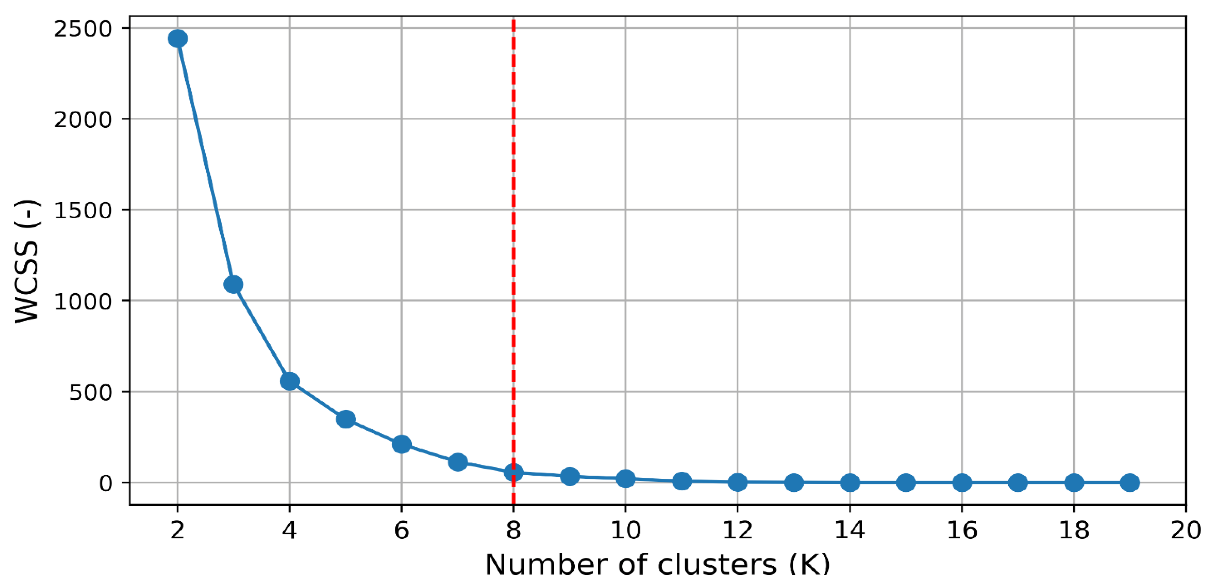
To determine the optimal values of K, this study uses the Elbow method. This method is a popular technique used in K-means clustering to determine the optimal number of clusters, K, for a given dataset. It involves evaluating the within-cluster sum of squares (WCSS) metric, which quantifies the compactness or tightness of clusters [27,28,29,30]. The Elbow method proceeds by computing the WCSS for different values of K and plotting them against the number of clusters. The resulting plot exhibits a characteristic shape resembling an elbow. The idea behind the method is to identify the point on the plot where the rate of decrease in the WCSS starts to diminish significantly, forming the “elbow”. This point indicates a trade-off between capturing more variance within clusters (a smaller WCSS) and avoiding excessive complexity (a larger K). The K value corresponding to the elbow point is often considered a reasonable choice for the number of clusters, striking a balance between model simplicity and cluster quality.

2.2.2. Decision Tree Classification Algorithm (Module II)

A decision tree (DT) is a popular machine learning algorithm used for both regression and classification tasks [31]. It is a supervised learning method that builds a predictive model in the form of a tree-based structure wherein each internal node represents a feature or attribute, each branch represents a decision rule, and each leaf node represents a class label or a predicted value (see Figure 1c). The goal of a DT classifier is to create an optimal tree that can efficiently partition the input data based on the feature values, ultimately leading to accurate predictions. The process of building a DT involves recursively splitting the data based on different features and their values, with the objective of maximizing the information gain or minimizing the impurity at each step [20,31]. There are different algorithms and strategies for constructing DT, such as Iterative Dichotomies 3 (ID3), a Successor of ID3 (C4.5), and Classification and Regression Trees (CART) [20]. These algorithms employ various criteria to determine the best splitting point such as Entropy, Gini impurity, or Information gain [32,33]. The splitting criteria help in selecting the feature that provides the most discriminatory power and leads to the greatest reduction in impurity. In this paper, the Gini index is used to evaluate the quality of a potential split when constructing a DT. It quantifies the probability of misclassifying a randomly selected element in a node if it were randomly assigned a class label according to the distribution of class labels in that node [34]. Mathematically, the Gini index is calculated as follows:
Gini = 1 ( p 1 2 + p 2 2 + + p g 2 )
where p g   comprises the probabilities of each class label in the node.
In general, the DT model is easy to understand and interpret as the resulting tree structure can be visualized and explained. The DTs can handle both numerical and categorical features, and they can also handle missing values by assigning probabilities to different outcomes. Moreover, DTs can capture non-linear relationships between features and target variables, and they can be used for feature selection as the most important features tend to appear near the roots of the trees.

2.2.3. Evaluation Metrics

Precision, Recall, and F1-score are evaluation metrics commonly used in classification tasks to assess the performance of a machine learning model. They provide insights into a model’s accuracy, completeness, and overall effectiveness in making predictions [35]. Precision is the measure of the model’s ability to correctly identify positive instances out of the total number of instances predicted as positive. It focuses on the accuracy of the positive predictions (Equation (3)).
Precision = TP   TP   +   FP
Here, TP (True Positives) represents the number of correctly predicted positive instances, and FP (False Positives) represents the number of instances that are predicted as positive but are actually negative. Precision is particularly useful when the cost of false positives is high and you want to minimize the number of false alarms or incorrect positive predictions. Recall, also known as sensitivity or true positive rate, measures the model’s ability to correctly identify positive instances out of the total number of actual positive instances. It focuses on the completeness of positive predictions (Equation (4)).
Recall = TP   TP   +   FN
Here, FN (False Negatives) represents the number of instances that are positive but predicted as negative. The Recall is especially valuable when the cost of false negatives is high and you want to minimize the number of missed positive instances or false negatives. The F1-score combines Precision and Recall into a single metric that balances both measures. It is the harmonic means of Precision and Recall, and provides a balanced evaluation of the model’s performance (Equation (5)).
F 1 - score = 2 × Precision   ×   Recall Precision   +   Recall
The F1-score ranges from 0 to 1, where 1 represents perfect Precision and Recall and 0 indicates poor performance in either Precision or Recall. The F1-score is particularly useful when we want to find a balance between Precision and Recall as it considers both metrics simultaneously. These metrics are widely used together to assess the performance of a classifier. However, it is important to note that their relative importance depends on the specific problem and the associated costs of false positives and false negatives.

2.2.4. Data

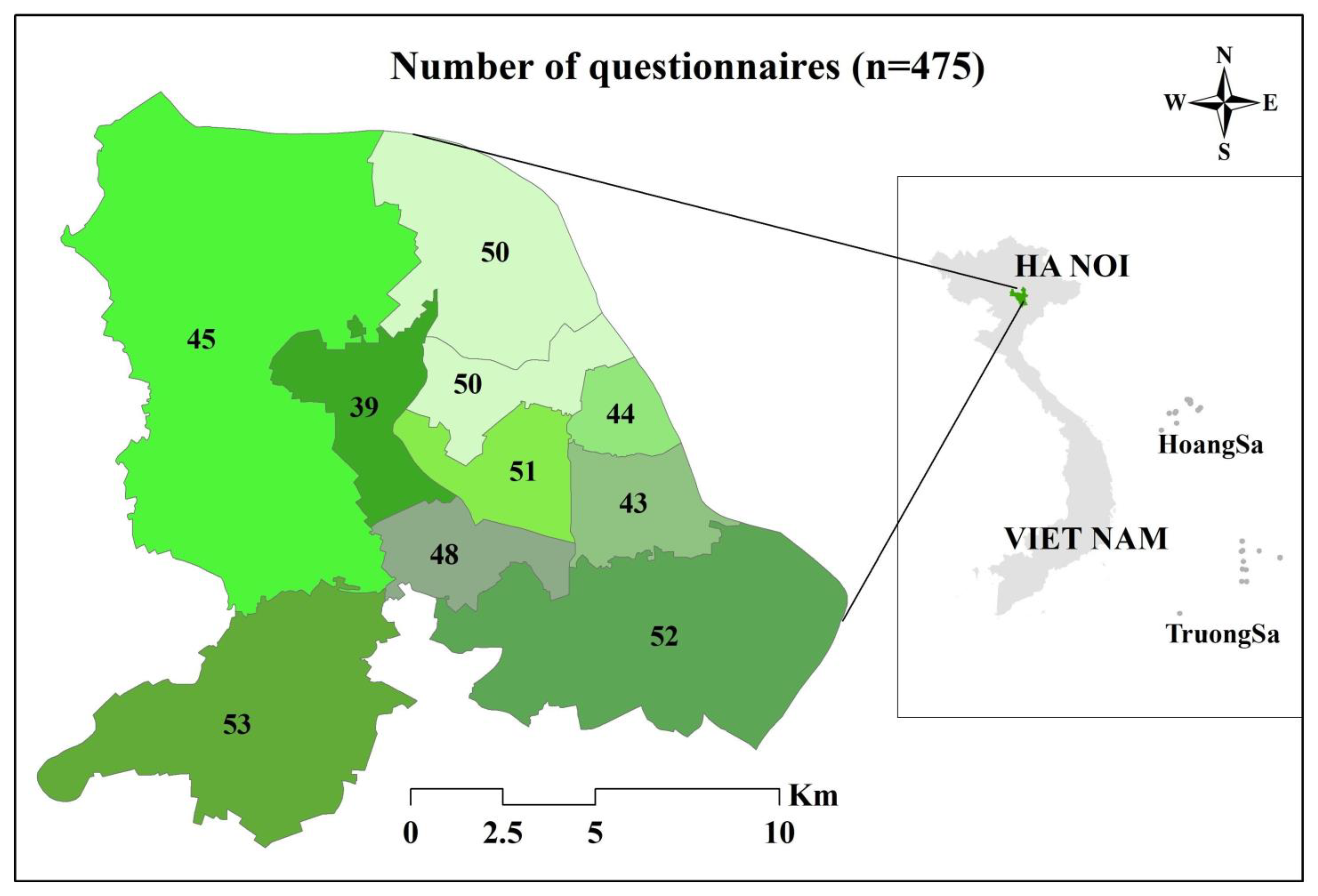
For this study, we utilized the same dataset on air pollution issues in Hanoi that was previously used by [7] to build the CVML model. In November 2019, we chose to employ a face-to-face interview method to survey the residents of Hanoi over a period of three weeks. To ensure that there would be no potential confusion or misunderstandings between interviewers and prospective respondents, we conducted two pilot studies to thoroughly examine the questionnaire. Our goal was to guarantee clarity and understanding before proceeding with the official interviews. To recruit participants for our survey, we opted for a stratified random sampling technique. This approach, categorized as a probability sampling method, is renowned for its effectiveness in minimizing sample bias when compared to the simpler random sampling method. By utilizing stratified random sampling, we sought to achieve a more representative and accurate depiction of the population under study. Hanoi’s central urban area comprises 12 central districts. However, due to budget limitations, we focused our research on 11 districts, intentionally excluding the Long Bien district. The decision to omit Long Bien was based on its geographical location, as it is situated the furthest from the city center and is positioned on the opposite side of the Red River (Figure 3). Within each of the selected districts, we proceeded to randomly select 40–50 local individuals from the main streets. In total, our efforts resulted in successfully conducting interviews with a sample size of 475 local individuals.
Table 1 provides the descriptive statistics for all variables used in this study. We have selected four independent variables ( x sur ) that possess the characteristics of being common and easily accessible. These variables will be utilized to examine their potential impact on the dependent variable ( y sur ), which represents the respondents’ willingness to pay. This dataset is used to train and test the CVML model, which can be applied to predict willingness to pay by building independent variables from the available data ( x obs ).

3. Results of Model Development

3.1. The K-Means Cluster (Module I)

Figure 4 showcases the application of the Elbow method to determine the ideal number of clusters (K) for a K-means clustering algorithm. This method aids in selecting the appropriate value of K by evaluating the variance explained as a function of the number of clusters. The plot depicts the number of clusters on the x-axis and the corresponding measure of variance or distortion on the y-axis. Distortion or the within-cluster sum of squares (WCSS) is commonly used as the metric to assess the quality of the clustering. As the number of clusters increases, the WCSS tends to decrease since more clusters allow for a better fit of the data points. However, at a certain point, the rate of decrease in WCSS begins to diminish, resulting in a bend or “elbow” in the plot. In this specific figure, the elbow point is observed at K = 8, indicating that the inclusion of additional clusters beyond this point does not significantly reduce the WCSS. The elbow represents a trade-off between capturing more detailed patterns within clusters and avoiding overfitting or excessive fragmentation. By selecting K = 8, we strike a balance between granularity and simplicity, achieving a meaningful level of cluster differentiation without creating an overly complex or fragmented clustering solution. The Elbow method provides a data-driven approach to guide the selection of the optimal number of clusters in K-means clustering, aiding in the interpretation and application of the results. It allows for efficient clustering by identifying the number of clusters that best capture the underlying structure of the data.
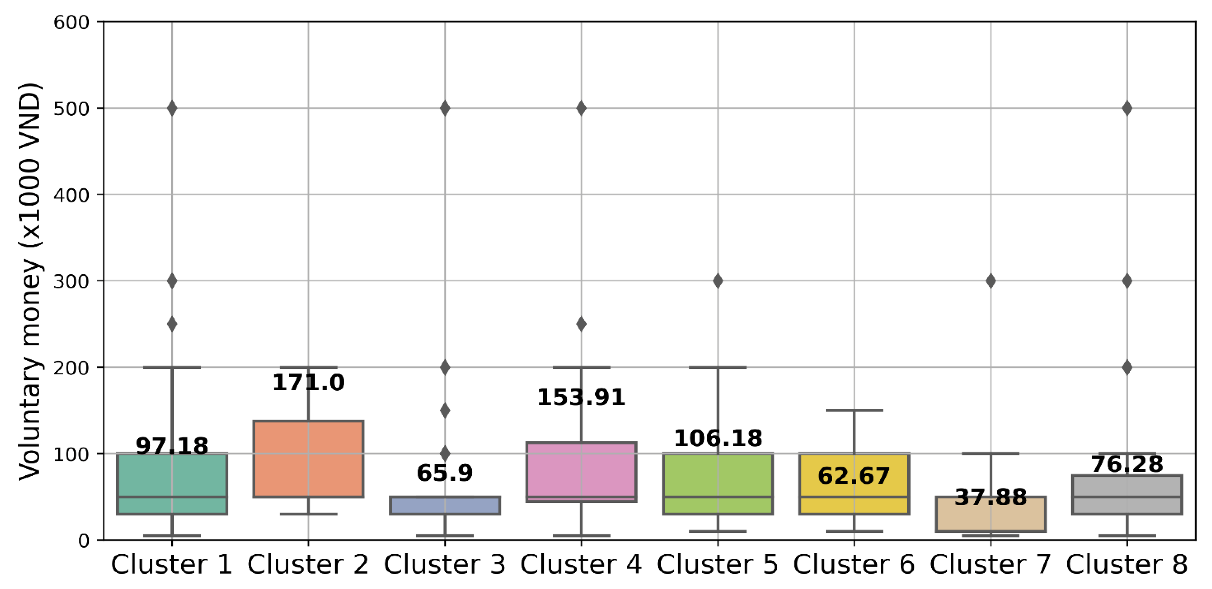
After applying the Elbow method, which determined that K = 8 was the optimal number of clusters for the given dataset, K-means clustering was performed, resulting in eight distinct groups. Figure 5 illustrates the average “voluntary money” value for each cluster. Notably, Group 4 stands out with a remarkable mean voluntary money value of 153.91 (×1000 VND), indicating a strong inclination towards significant individual contributions. Similarly, Group 2 emerges as one of the highest contributing segments, with a mean value of 171.00 (×1000 VND). In contrast, Group 7 exhibits the lowest mean value, 37.88 (×1000 VND), suggesting relatively lower levels of contribution compared to the other groups. The observed differences between groups are significant, reaching up to 4.5 times. This substantial variation highlights the potential for substantial errors if the mean method is solely used to estimate voluntary donations. Consequently, it becomes necessary to develop a predictive model to estimate the contribution amount for each group when estimating voluntary donations in a larger sample. By employing such a model, more accurate and reliable estimates can be obtained, accounting for the distinct contribution patterns exhibited by each group.
In Module II, the focus is on utilizing variable x sur , which represents the input features, and variable y sur , which represents the average voluntary money values of the eight groups. The goal is to construct a classification prediction model capable of predicting and estimating voluntary money when applied to a large number of samples.

3.2. The Classification Prediction Model (Module II)

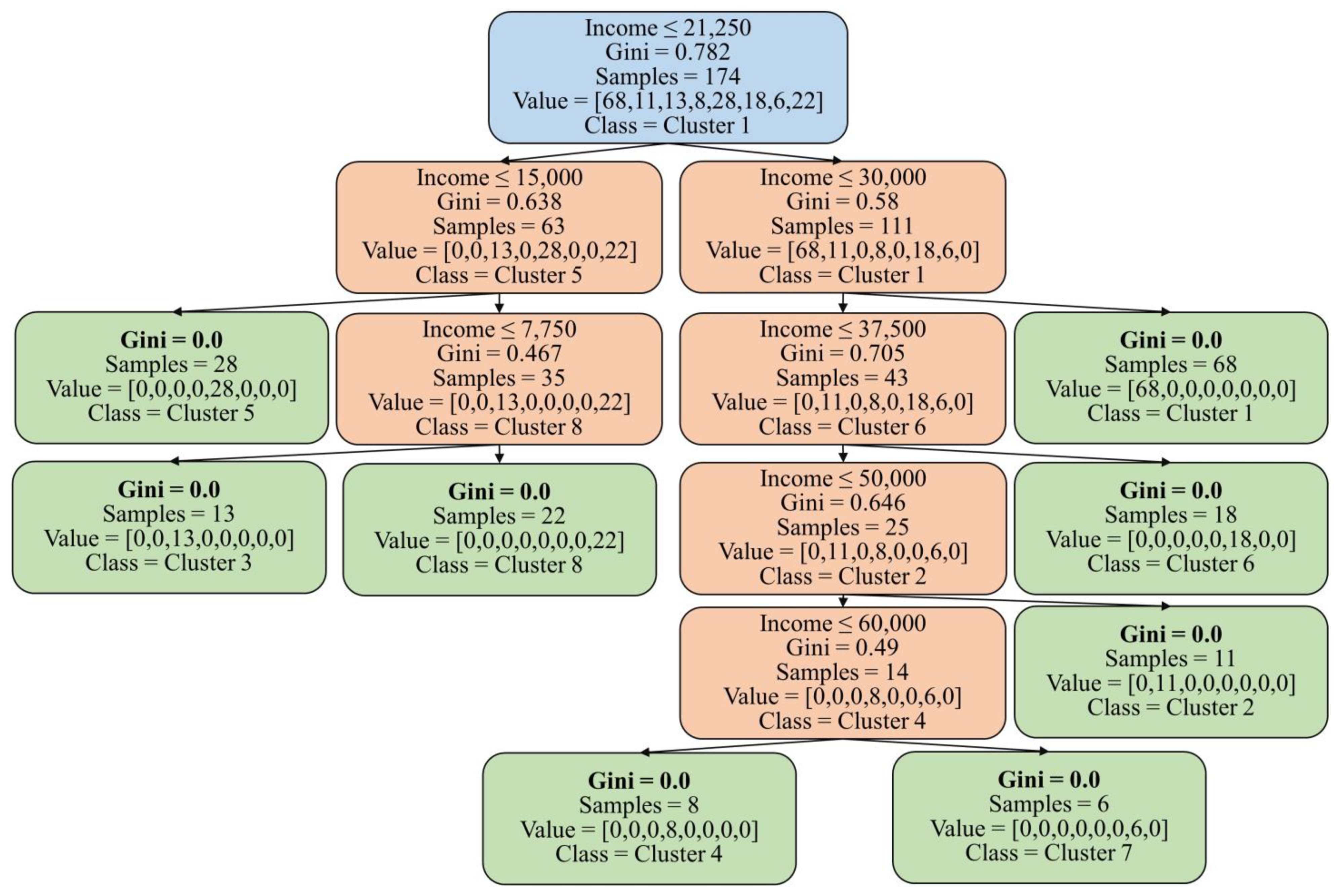
To train the DT model, 50% of the dataset is used. The model with a maximum depth of 5 is chosen as it provides sufficient complexity to classify all the groups in the dataset. This means that the DT, with its five levels of splits, can effectively capture the underlying patterns and relationships necessary to classify the samples into their respective groups. Importantly, after these five levels of splits, it is worth noting that all eight groups in the training dataset are successfully classified with a Gini index of 0. This signifies that the decision tree model has accurately captured the distinct characteristics and patterns of each group, resulting in pure nodes at the end of the fifth level. Achieving a Gini index of 0 for all eight groups indicates the absence of impurity or the mixing of samples from different groups within their respective nodes (see Figure 6). This showcases the model’s effectiveness in accurately separating and classifying the samples. By achieving a Gini index of 0 for all eight groups after five levels of splits, the decision tree classification model of Module II demonstrates its strong predictive power and ability to correctly assign new samples to their appropriate groups based on their input features.
To evaluate the model’s performance and assess both its predictive ability and the presence of overfitting, we conduct testing on the test dataset (50% of the dataset). The test dataset serves as an independent set of samples that were not used during the model’s training process. During the testing phase, the model is applied to the test dataset and the results are presented using a confusion matrix (Figure 7). The confusion matrix provides a comprehensive overview of the model’s performance by showing the counts of true positive, true negative, false positive, and false negative predictions.
In this detailed confusion matrix, we explore the performance of a classification model designed to classify data into eight distinct classes. The matrix provides valuable insights into the accuracy and efficacy of the model’s predictions. The rows in the matrix correspond to the actual classes while the columns represent the predicted classes. Each cell in the matrix indicates the number of instances belonging to a specific true class and classified as a specific predicted class. This visual representation allows us to analyze both correct and incorrect predictions across the various classes. The diagonal cells from the top-left to the bottom-right of the matrix display the number of correctly classified instances for each class. Higher values along this diagonal indicate higher levels of accuracy and effectiveness in the model’s predictions.
Upon evaluating the model’s performance on the test dataset, we observe that the model successfully predicts all clusters except for cluster 2, which has only one correct prediction out of four values. This indicates that the model performs well in accurately classifying most of the clusters, but there may be some challenges or complexities specifically associated with cluster 5.
Table 2 presents the Precision, Recall, and F1-score values of the decision tree (DT) model while working on the test set, providing a detailed evaluation of its performance. Clusters 1, 3, 4, 6, 7, and 8 demonstrate perfect Precision, Recall, and F1-scores of 1, indicating accurate predictions for all instances within these clusters. They have respective instance counts of 58, 29, 14, 7, 20, and 19. Cluster 2 exhibits a lower Recall of 0.25, indicating that only 25% of the values that need to be forecasted are correctly predicted by the model. The Precision is reported as 1, indicating that all the predictions made for this cluster are accurate. Cluster 2 comprises only 4 instances. Cluster 5 shows a Precision of 0.88, indicating that 12% of the predictions made for this cluster are mistakenly classified by other groups. However, the Recall is 1, indicating that all the values that belong to this cluster are correctly predicted. By analyzing these performance metrics, we can gain insights into the strengths and weaknesses of the decision tree model’s classification performance for each specific cluster. These metrics enable us to assess the model’s accuracy and identify areas for potential improvement such as addressing the misclassification issue in Cluster 2 and 5 to improve precision.
Overall, the decision tree model demonstrates a high average accuracy of approximately 98%. The model successfully predicts most clusters accurately, with only clusters 2 and 5 experiencing lower accuracy. The primary reason for this could be attributed to the small number of samples available for these clusters, resulting in limited information and potential difficulties in capturing their underlying patterns. The limited sample size in clusters 2 and 5 may lead to the insufficient representation of their characteristics during the model training process. As a result, the model might struggle to generalize well for these clusters, leading to lower accuracy in their predictions. To address this issue and improve the accuracy for clusters 2 and 5, it is recommended to acquire additional training and test data specifically targeting these clusters. By incorporating more samples, the model can gain a better understanding of their unique patterns and enhance its predictive performance.

4. Testing the Applicability of the CVML Method

The study found that by utilizing only four commonly available independent variables ( x sur ), the CVML model demonstrated promising results in predicting the respondents’ willingness to pay as indicated by the test dataset (Section 2.2.2). This outcome presents an opportunity to apply the CVML model for predicting willingness to pay by leveraging existing data, thereby reducing the time and costs associated with conducting extensive surveys.
In this study, we aimed to apply the CVML model to predict the respondents’ willingness to pay using available data ( x obs ) published by [36]. Additionally, we compared the predicted values obtained from the CVML model with the estimated results generated by the CV method, as presented in the study conducted by [7,37,38]. It is important to note that both the CVML model and the CV method utilized the same dataset for their analyses. By comparing the predicted values from these two approaches, we can assess the accuracy and efficiency of the CVML model in predicting willingness to pay in relation to the established CV method, providing valuable insights into the predictive capabilities of the CVML model using the available dataset.
In the published dataset titled “A Data Collection on Secondary School Students’ STEM Performance and Reading Practices in an Emerging Country” [36], there are a total of 42 variables and 4966 respondents. For the purpose of the CVML model, we filter out four specific variables from this dataset. We then proceed to standardize the values of these variables to ensure that they are on the same scale as the training dataset. After filtering and standardization, the resulting dataset consists of 714 matching lines, with the four variables of interest referred to as x obs . These variables are now ready to be used as inputs for the CV and CVML models to predict the respondents’ willingness to pay.
Table 3 presents the results of WTP estimation using CV and CVML. According to the CV method, for dataset I, the estimated willingness to pay for reducing air pollution ranged from USD 4.6 to USD 6.04 per household [7]. With a total of 714 households, the estimated total for air pollution control would range from USD 3284.4 to USD 4312.56. On the other hand, for dataset II, the prediction of the CVML method yielded a result of USD 3984.12.

5. Discussion

The CVML method is developed with the aim to improve WTP estimates for improved environment quality. Briefly speaking, this method employs the CV data that have been carefully designed and collected by the CV method. These data are used as the input for ML to develop the desired model, which is then rigorously validated and used to determine the WTP values based on the new data. The attributes and conditions of the method are further discussed below.
Firstly, CVML can enhance WTP estimate accuracy (Table 4). To be specific, when the predictive model is tested, it is deemed highly efficient since it can predict outcomes with 98% accuracy. It is noted that forecasting models are acceptable even when the accuracy level is only around 70%. In addition, the estimated willingness to pay for air pollution mitigation ranged from USD 4.6 to USD 6.04 per household, resulting in an estimated total for controlling air pollution ranging from USD 3284.4 to USD 4312.56 (with an average of USD 3798.48), whereas the CVML method predicted a result of USD 3984.12, which is 4.8% higher than the average estimated by the CV method (Table 3). This indicates that the CVML method predicted a slightly higher value for willingness to pay compared to the CV method’s average estimation. The difference in the predicted values suggests that the CVML model may have accounted for additional factors or incorporated different variables, leading to a slightly higher prediction. This finding highlights the potential of the CVML model to provide improved predictions compared to the traditional CV method in estimating both willingness to pay for air pollution control as well as other fields.
Secondly, CVML can save money. The cost of science has become a major concern for scientists around the world, particularly in developing countries [39]. While conducting research is time-consuming and costly, researchers are confronted with the fact that research funding is dwindling owing to government cutbacks [40,41,42]. Because CVML can make use of open data platforms, the method can benefit significantly from the current trend of open science [43]. This means that the method can help users (e.g., scientists, scholars, etc.) reduce cost considerably. This attribute of CVML is similar to that of the Bayesian Mindsponge Framework (BMF), a novel method that has been introduced recently for social and psychological research [44]. More importantly, CVML can help to increase scientific productivity in terms of both quality and quantity. This can ultimately help to reduce inequalities in scientific publishing among institutes and nations in the long run. [45,46].
Thirdly, CVML can be used to determine WTP that can be applied to larger areas. In this study, CVML was performed based on CV data in Hanoi and new data surveyed in the Ninh Binh province. These data came from the study “A Data Collection on Secondary School Students’ STEM Performance and Reading Practices in an Emerging Country” [36]. As a result, the estimated WTP could be applied to Vietnam’s Red River Delta, which is much larger than the Hanoi area. It is noted that the scale of application has a close relationship with the cost aforementioned above. If CVML can use more data from a larger area, it means that the method can help users save more money. Conversely, if CVML is used to apply WTP to a smaller scale, the reduced cost will be lower.
There are some key conditions of CVML that should be noted. The first one refers to the quality of the data used to train the machine learning model. The data should be representative of the population of interest. If the data are not representative, then CVML may not be able to accurately estimate WTP for the population of interest. From this view, CVML coupled with the stratified random sampling approach should be well designed to maximize the benefits of the method. In addition, the data should be accurate and reliable. If the data are not accurate, then the machine learning model may not be able to accurately estimate WTP. Furthermore, the data should be sufficiently large. If the data are not sufficiently large, then the machine learning model may not be able to learn the patterns in the data that are necessary to accurately estimate WTP. In addition to these conditions, the quality of the data used to train the machine learning model can also be influenced by the way in which the data are collected and processed. For example, if the data are collected in a biased way, then CVML may learn the bias in the data and produce biased WTP estimates. In this sense, a well-designed CV study can improve the quality of the CV data, which can ultimately lead to more accurate WTP estimates using CVML. The second one is the type of machine learning algorithm used. The type of machine learning algorithm used can influence the quality of WTP estimation for a number of reasons. First, different machine learning algorithms are better suited for different types of data. For example, some machine learning algorithms are better at dealing with categorical data (e.g., decision trees, random forests, etc.), while others are better at dealing with continuous data (e.g., linear regression, polynomial regression, etc.). Second, different machine learning algorithms are more complex than others. More complex machine learning algorithms can learn more complex patterns in the data, but they can also be more prone to overfitting. Third, different machine learning algorithms require different amounts of data to train. Some machine learning algorithms can be trained with relatively small datasets, while others require large datasets.

6. Conclusions

Contingent valuation (CV) is a useful tool, but it has limitations that make it less powerful. This study is one of the first efforts to develop and advocate for the use of contingent valuation machine learning (CVML) analytics. To illustrate, we used the air pollution dataset from Hanoi, the K-means cluster (model I), and a decision tree model (model II) to develop a desired model. This model was then used to estimate the willingness to pay (WTP) value from the published dataset. The high accuracy of the developed model suggests that CVML can improve WTP estimates. The CVML model has the potential to become more reliable when applied to larger datasets. The method is also efficient because it relies on simple and easily accessible input data. This means that public sources and data from previous studies can be used, which reduces the need for extensive and costly data collection efforts. Additionally, the data required for the CVML model are fundamental and can be easily disseminated, which aligns with the digital data development strategies of developing countries such as Vietnam. This compatibility with basic data sources facilitates the implementation and scalability of the method, making it a powerful tool for socioeconomic studies. Overall, CVML advances the method of estimating WTP because of its low cost and high performance. When applied to larger datasets and in conjunction with the digital data strategies adopted by developing countries, CVML can support decision-makers in improving the financial resources available to maintain and/or further support many environmental programs in the coming years.

Author Contributions

Conceptualization, V.Q.K. and D.T.T.; methodology, V.Q.K. and D.T.T.; software, V.Q.K. and D.T.T.; validation, V.Q.K. and D.T.T.; formal analysis, V.Q.K. and D.T.T.; resources, V.Q.K. and D.T.T.; data curation, V.Q.K. and D.T.T.; writing—original draft preparation, V.Q.K. and D.T.T.; writing—review and editing, V.Q.K. and D.T.T.; visualization, V.Q.K. and D.T.T.; supervision, V.Q.K. All authors have read and agreed to the published version of the manuscript.

Funding

This research received no external funding.

Data Availability Statement

Not applicable.

Acknowledgments

We are deeply grateful to my parents and aunt for raising and educating us over the last years. We also like to thank everyone who contributed to and/or participated in this study. Specially, we would like to express our sincere thanks to the anonymous reviewers who provided constructive comments to improve the paper’s quality.

Conflicts of Interest

The authors declare no conflict of interest.

References

  1. Atteridge, A. Will Private Finance Support Climate Change Adaptation in Developing Countries? Historical Investment Patterns as a Window on Future Private Climate Finance. 2011, 5. Available online: https://www.sei.org/publications/will-private-finance-support-climate-change-adaptation-in-developing-countries-historical-investment-patterns-as-a-window-on-future-private-climate-finance/ (accessed on 1 August 2023).
  2. Buso, M.; Stenger, A. Public-Private Partnerships as a Policy Response to Climate Change. Energy Policy 2018, 119, 487–494. [Google Scholar] [CrossRef]
  3. Champ, P.A.; Boyle, K.J.; Brown, T.C. A Primer on Nonmarket Valuation; Kluwer Academic Publishers: Norwell, MA, USA, 2017. [Google Scholar]
  4. Carson, R.T.; Hanemann, W.M. Chapter 17 Contingent Valuation. In Handbook of Environmental Economics; Elsevier: Amsterdam, The Netherlands, 2005; Volume 2, pp. 821–936. [Google Scholar] [CrossRef]
  5. Venkatachalam, L. The Contingent Valuation Method: A Review. Environ. Impact Assess. Rev. 2004, 24, 89–124. [Google Scholar] [CrossRef]
  6. Kamri, T. Willingness to Pay for Conservation of Natural Resources in the Gunung Gading National Park, Sarawak. Procedia-Soc. Behav. Sci. 2013, 101, 506–515. [Google Scholar] [CrossRef] [Green Version]
  7. Khuc, V.Q.; Nong, D.; Vu, P.T. To Pay or Not to Pay That Is the Question—For Air Pollution Mitigation in a World’s Dynamic City: An Experiment in Hanoi, Vietnam. Econ. Anal. Policy 2022, 74, 687–701. [Google Scholar] [CrossRef]
  8. Báez, A.; Herrero, L.C. Using Contingent Valuation and Cost-Benefit Analysis to Design a Policy for Restoring Cultural Heritage. J. Cult. Herit. 2012, 13, 235–245. [Google Scholar] [CrossRef]
  9. Khuc, V.Q.; Alhassan, M.; Loomis, J.B.; Tran, T.D.; Paschke, M.W. Estimating Urban Households’ Willingness-to-Pay for Upland Forest Restoration in Vietnam. Open J. For. 2016, 6, 191–198. [Google Scholar] [CrossRef] [Green Version]
  10. Wang, T.; Wang, J.; Wu, P.; Wang, J.; He, Q.; Wang, X. Estimating the Environmental Costs and Benefits of Demolition Waste Using Life Cycle Assessment and Willingness-to-Pay: A Case Study in Shenzhen. J. Clean. Prod. 2018, 172, 14–26. [Google Scholar] [CrossRef]
  11. Masud, M.M.; Junsheng, H.; Akhtar, R.; Al-Amin, A.Q.; Kari, F.B. Estimating Farmers’ Willingness to Pay for Climate Change Adaptation: The Case of the Malaysian Agricultural Sector. Environ. Monit. Assess. 2015, 187, 38. [Google Scholar] [CrossRef]
  12. Nguyen, A.-T.; Tran, M.; Nguyen, T.; Khuc, Q. Using Contingent Valuation Method to Explore the Households’ Participation and Willingness-to-Pay for Improved Plastic Waste Management in North Vietnam. In Contemporary Economic Issues in Asian Countries: Proceeding of CEIAC 2022; Nguyen, A.T., Pham, T.T., Song, J., Lin, Y.L., Dong, M.C., Eds.; Springer: Singapore, 2023; Volume 2, pp. 219–237. [Google Scholar]
  13. Carson, R.T. Contingent Valuation:A User’s Guide. Environ. Sci. Technol. 2000, 34, 1413–1418. [Google Scholar] [CrossRef] [Green Version]
  14. Lopes, A.F.; Kipperberg, G. Diagnosing Insensitivity to Scope in Contingent Valuation. Environ. Resour. Econ. 2020, 77, 191–216. [Google Scholar] [CrossRef]
  15. Whitty, J.A. Insensitivity to Scope in Contingent Valuation Studies: New Direction for an Old Problem. Appl. Health Econ. Health Policy 2012, 10, 361–363. [Google Scholar] [CrossRef]
  16. Fernández, C.; León, C.J.; Steel, M.F.J.; Vázquez-Polo, F.J. Bayesian Analysis of Interval Data Contingent Valuation Models and Pricing Policies. J. Bus. Econ. Stat. 2004, 22, 431–442. [Google Scholar] [CrossRef]
  17. Carandang, M.G.; Calderon, M.M.; Camacho, L.D.; Dizon, J.T. Parametric and Non-Parametric Models To Estimate Households’ Willingness To Pay For Improved Management of Watershed. J. Environ. Sci. Manag. 2008, 11, 68–78. [Google Scholar]
  18. Mead, W.J. Review and analysis of state-of-the art contingent valuation studies. In Contingent Valuation: A Critical Assessment; Hausman, J.A., Ed.; Elsevier: Amsterdam, The Netherlands, 1993; pp. 305–337. [Google Scholar]
  19. Carson, R.T.; Flores, N.E.; Meade, N.F. Contingent Valuation: Controversies and Evidence. Environ. Resour. Econ. 2001, 19, 173–210. [Google Scholar] [CrossRef]
  20. Mahesh, B. Machine Learning Algorithms—A Review. Int. J. Sci. Res. 2020, 18, 381–386. [Google Scholar] [CrossRef]
  21. Shrestha, A.; Mahmood, A. Review of Deep Learning Algorithms and Architectures. IEEE Access 2019, 7, 53040–53065. [Google Scholar] [CrossRef]
  22. Shyu, M.; Chen, S.; Iyengar, S.S. A Survey on Deep Learning: Algorithms, Techniques. ACM Comput. Surv. 2018, 51, 1–36. [Google Scholar]
  23. Brownlee, J. A Gentle Introduction to Ensemble Learning Algorithms. Available online: https://machinelearningmastery.com/tour-of-ensemble-learning-algorithms/ (accessed on 2 August 2023).
  24. MacQueen, J. Some Methods for Classification and Analysis of Multivariate Observations. In Proceedings of the 5th Berkley Symposium on Mathematical Statistics and Probability, Berkeley, CA, USA, 21 June–18 July 1965; University of California Press: Oakland, CA, USA, 1967; pp. 281–297. [Google Scholar]
  25. Žalik, K.R. An efficient k′-means clustering algorithm. Pattern Recognit. Lett. 2008, 29, 1385–1391. [Google Scholar] [CrossRef]
  26. Rana, S.; Jasola, S.; Kumar, R. A Hybrid Sequential Approach for Data Clustering Using K-Means and Particle Swarm Optimization Algorithm. Int. J. Eng. Sci. Technol. 2010, 2, 167–176. [Google Scholar] [CrossRef] [Green Version]
  27. Brusco, M.J.; Steinley, D. A Comparison of Heuristic Procedures for Minimum Within-Cluster Sums of Squares Partitioning. Psychometrika 2007, 72, 583–600. [Google Scholar] [CrossRef]
  28. Hartigan, J.A.; Algorithm, M.A.W. AS 136: A K-Means Clustering Algorithm. J. R. Stat. Soc. Ser. B Methodol. 1979, 28, 100–108. [Google Scholar]
  29. Krzanowski, W.J.; Lai, Y.T. A Criterion for Determining the Number of Groups in a Data Set Using Sum-of-Squares Clustering. Biometrics 1988, 44, 23. [Google Scholar] [CrossRef]
  30. Thorndike, R.L. Who Belongs in the Family? Psychometrika 1953, 18, 267–276. [Google Scholar] [CrossRef]
  31. Swain, P.H.; Hauska, H. Decision Tree Classifier: Design and Potential. IEEE Trans. Geosci. Electron. 1977, 15, 142–147. [Google Scholar] [CrossRef] [Green Version]
  32. Cheushev, V.; Simovici, D.A.; Shmerko, V.; Yanushkevich, S. Functional Entropy and Decision Trees. In Proceedings of the International Symposium on Multiple-Valued Logic, Fukuoka, Japan, 29 May 1998; pp. 257–262. [Google Scholar]
  33. Molala, R. Entropy, Information Gain, Gini Index—The Crux of a Decision Tree. Available online: https://www.clairvoyant.ai/blog/entropy-information-gain-and-gini-index-the-crux-of-a-decision-tree (accessed on 10 July 2023).
  34. Tangirala, S. Evaluating the Impact of GINI Index and Information Gain on Classification Using Decision Tree Classifier Algorithm. Int. J. Adv. Comput. Sci. Appl. 2020, 11, 612–619. [Google Scholar] [CrossRef] [Green Version]
  35. Goutte, C.; Gaussier, E. A Probabilistic Interpretation of Precision, Recall and F-Score, with Implication for Evaluation. In Advances in Information Retrieval. ECIR 2005. Lecture Notes in Computer Science; Springer: Berlin/Heidelberg, Germany, 2005; Volume 3408, pp. 345–359. [Google Scholar] [CrossRef]
  36. Vuong, Q.H.; La, V.P.; Ho, M.T.; Pham, T.H.; Vuong, T.T.; Vuong, H.M.; Nguyen, M.H. A Data Collection on Secondary School Students’ Stem Performance and Reading Practices in an Emerging Country. Data Intell. 2021, 3, 336–356. [Google Scholar] [CrossRef]
  37. Khuc, V.Q.; Vu, P.T.; Luu, P. Dataset on the Hanoian Suburbanites’ Perception and Mitigation Strategies towards Air Pollution. Data Brief 2020, 33, 106414. [Google Scholar] [CrossRef]
  38. Vuong, Q.-H.; Phu, T.V.; Le, T.-A.T.; Van Khuc, Q. Exploring Inner-City Residents’ and Foreigners’ Commitment to Improving Air Pollution: Evidence from a Field Survey in Hanoi, Vietnam. Data 2021, 6, 39. [Google Scholar] [CrossRef]
  39. Vuong, Q. The (Ir)Rational Consideration of the Cost of Science in Transition Economies. Nat. Hum. Behav. 2018, 2, 41562. [Google Scholar] [CrossRef]
  40. Nwako, Z.; Grieve, T.; Mitchell, R.; Paulson, J.; Saeed, T.; Shanks, K.; Wilder, R. Doing Harm: The Impact of UK’s GCRF Cuts on Research Ethics, Partnerships and Governance. Glob. Soc. Chall. J. 2023, XX, 1–22. [Google Scholar] [CrossRef]
  41. Kakuchi, S. Universities Brace for More Cuts as Defence Spending Rises. Available online: https://www.universityworldnews.com/post.php?story=20230118144238399 (accessed on 2 August 2023).
  42. Collins, M. Declining Federal Research Is Hurting US Innovation. Available online: https://www.industryweek.com/the-economy/public-policy/article/21121160/declining-federal-research-undercuts-the-us-strategy-of-innovation (accessed on 1 August 2023).
  43. Vuong, Q.-H. Open Data, Open Review and Open Dialogue in Making Social Sciences Plausible. Sci. Data Update 2017. Available online: http://blogs.nature.com/scientificdata/2017/12/12/authors-corner-open-data-open-reviewand-open-dialogue-in-making-social-sciences-plausible/ (accessed on 1 August 2023).
  44. Nguyen, M.H.; La, V.P.; Le, T.T.; Vuong, Q.H. Introduction to Bayesian Mindsponge Framework Analytics: An Innovative Method for Social and Psychological Research. Methodsx 2022, 9, 101808. [Google Scholar] [CrossRef] [PubMed]
  45. Vuong, Q. Western Monopoly of Climate Science Is Creating an Eco-Deficit Culture. Available online: https://elc-insight.org/western-monopoly-of-climat (accessed on 2 August 2023).
  46. Xie, Y. “Undemocracy”: Inequalities in Science. Science 2014, 344, 809–810. [Google Scholar] [CrossRef] [PubMed] [Green Version]
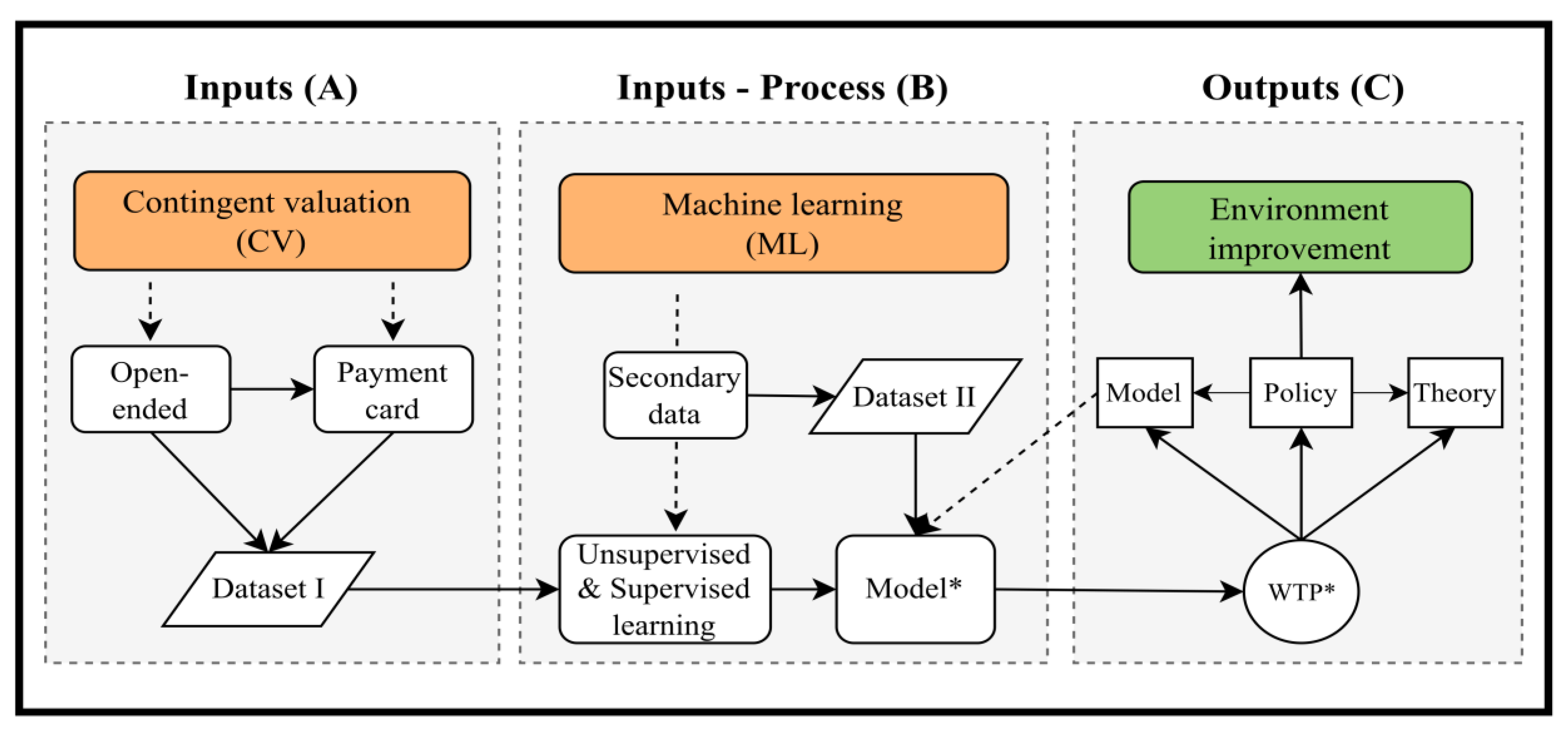
Figure 1. CVML analytics framework. Note: The framework is made up of three major components: inputs, processes, and outcomes. With the support of the machine learning method, the contingent valuation data is used as an input to develop the model (Block A). After the developed model has been well validated, it can be utilized to analyze data for the needs of the users (Block B). The estimated WTP would have numerous implications for model, theory, and policy (Block C). The asterisk (*) denotes the CVML model developed and its estimated WTP.
Urbansci 07 00084 g001
Figure 2. Hybrid machine-learning model framework. This framework is shown in (a), which includes two modules: (b) unsupervised (Module I) and (c) supervised learning (Module II).
Urbansci 07 00084 g002
Figure 3. Study area and number of questionnaires. Note: Different green color represents the number of questionnaires collected in each district (total n = 475).
Urbansci 07 00084 g003
Figure 4. Elbow method for choosing optimal values of K. Note: The blue line represents the WCSS value that changes with increasing the value of K, and the red dashed line represents the optimal K value selected.
Urbansci 07 00084 g004
Figure 5. Average voluntary money of each cluster. On each boxplot, the central mark indicates the median, and the bottom and the top edges of the box indicate the 25th and 75th percentiles, respectively. The diamond symbol represents the outliers.
Urbansci 07 00084 g005
Figure 6. Decision tree for the training process (Module II). The root node is symbolized by the blue box, while the decision node is depicted by the orange box, and the leaf node is exemplified by the green box.
Urbansci 07 00084 g006
Figure 7. Confusion matrix analysis of a decision tree model (Module II) for eight-cluster prediction.
Urbansci 07 00084 g007
Table 1. Descriptive table of variables.
VariablesDefinitions and MeasurementsMeanSD
x sur GenderGender of respondents. 1 = Male; 0 = Female0.5460.498
AgeAge of respondents. 1 = aged 10–18; 2 = aged 19–30; 3 = aged 31–40; 4 = aged 41–50; 5 = aged 51–60; 6 = aged above 603.6381.534
EducationRespondents’ highest educational levels attained. 1 = Secondary school or below; 2 = Highschool; 3 = Technical school/college degree; 4 = Bachelor’s Degree; 5 = Master’s Degree; 6 = Doctoral Degree0.5310.5
LogIncomeCommon logarithm of midpoints of the reported respondent’s household disposal income intervals (million VND per month)0.5460.498
y sur Willingness to payThe contribution values are 0, 5, 10, 20, 30, 50, 100, 150, 200, 250, 300, 350, 400, 450, 500, 1000, and above 1000 thousand Vietnam Dong (VND) (in US dollars, these levels are USD 0, USD 0.2, USD 0.4, USD 0.9, USD 1.3, USD 2.2, USD 4.3, USD 6.5, USD 8.7, USD 10.9, USD 13, 15.2, USD 17.4, USD 19.6, USD 21.7, USD 43.5, and above USD 43.5, respectively; USD 1∼23,000 VND)8707 (VND)12,232 (VND)
Table 2. Accuracy of DT model (Module II) for eight-cluster prediction.
PrecisionRecallF1-ScoreN
Cluster 111158
Cluster 210.250.44
Cluster 311129
Cluster 411114
Cluster 50.8810.9423
Cluster 61117
Cluster 711120
Cluster 811119
Table 3. Summary of results for estimated WTP.
DimensionsCVCVML
Sample size (dataset I)475475
WTPUSD 4.6 to USD 6.04-
New data (dataset II)714714
Total WTPUSD 3284.4 to USD 4312.56USD 3984.12
WTP *-USD 5.58
Source: [7] and own elaboration. Note: Asterisk (*) refers to the estimated WTP using CVML.
Table 4. Summary of attributes of CV and CVML.
DimensionsCVCVML
AccuracyAcceptable High     very high
CostHighVery small → Zero
Scale of applicationSmall (e.g., city, town)Large (e.g., regional, national)
Difficulty level when using the methodEasy → IntermediateIntermediate → hard
Conditions/factorsDesign (e.g., focus group, questionnaire, data frame, sample size, etc.)Quality of CV data (e.g., representativeness);
Machine learning algorithms (e.g., decision tree, logistic regression, etc.)
Source: own elaboration.
Disclaimer/Publisher’s Note: The statements, opinions and data contained in all publications are solely those of the individual author(s) and contributor(s) and not of MDPI and/or the editor(s). MDPI and/or the editor(s) disclaim responsibility for any injury to people or property resulting from any ideas, methods, instructions or products referred to in the content.