Article

The TRAX Light-Rail Train Air Quality Observation Project

1
Department of Atmospheric Sciences, University of Utah, Salt Lake City, UT 84112, USA
2
Pulmonary Division, School of Medicine, University of Utah, Salt Lake City, UT 84112, USA
3
Department of Life, Earth and Environmental Sciences, West Texas A&M University, Canyon, TX 79016, USA
*
Author to whom correspondence should be addressed.
Urban Sci. 2019, 3(4), 108; https://doi.org/10.3390/urbansci3040108
Submission received: 10 November 2019 / Revised: 29 November 2019 / Accepted: 29 November 2019 / Published: 1 December 2019
(This article belongs to the Special Issue Technologies and Humanities for Smart Cities)

Abstract

:
Observing air quality from sensors onboard light rail cars in Salt Lake County, Utah began as a pilot study in 2014 and has now evolved into a five-year, state-funded program. This metropolitan region suffers from both elevated ozone levels during summer and high PM2.5 events during winter. Pollution episodes result predominantly from local anthropogenic emissions but are also impacted by regional transport of dust, chemical precursors to ozone, and wildfire smoke, as well as being exacerbated by the topographical features surrounding the city. Two electric light-rail train cars from the Utah Transit Authority light-rail Transit Express (“TRAX”) system were outfitted with PM2.5 and ozone sensors to measure air quality at high spatial and temporal resolutions in this region. Pollutant concentration data underwent quality control procedures to determine whether the train motion affected the readings and how the sensors compared against regulatory sensors. Quality assurance results from data obtained over the past year show that TRAX Observation Project sensors are reliable, which corroborates earlier preliminary validation work. Three case studies from summer 2019 are presented to illustrate the strength of the finely-resolved air quality observations: (1) an elevated ozone event, (2) elevated particulate pollution resulting from 4th of July fireworks, and (3) elevated particle pollution during a winter time inversion event. The mobile observations were able to capture spatial gradients, as well as pollutant hotspots, during both of these episodes. Sensors have been recently added to a third light rail train car, which travels on a north–south oriented rail line, where air quality was unable to be monitored previously. The TRAX Observation Project is currently being used to provide reliable pollutant data for health studies and inform urban planning efforts. Links to real-time data displays and updated information on the quality-controlled data from this study are available on the webpage for the Department of Atmospheric Sciences at the University of Utah.

Graphical Abstract

1. Introduction

1.1. Motivation

1.1.1. Air Quality in the Salt Lake Valley, Utah

The Wasatch Front is the largest metropolitan area in the state of Utah, within which approximately 35% of the state’s population reside in the Salt Lake Valley (SLV) [1]. Salt Lake City (SLC), the state capital with a population of 200,000, lies within the SLV (Figure 1). The SLV is a mountain basin bounded by the Wasatch Mountains to the east, Oquirrh Mountains to the west, the Traverse Mountains to the south, and the opening to the Great Salt Lake to the northwest.
The terrain surrounding the SLV increases the vulnerability of residents to poor air quality, particularly during winter and summer. Ground-level particulate matter becomes trapped for up to two weeks when winter cold-air pools are present that result from stable conditions aloft and cold air near the snow-covered ground [2]. During long summer days, clear skies and light winds contribute to favorable conditions for elevated photochemical production and accumulation of ground level ozone [3]. Smoke from local wildfires, as well as those throughout the western United States, can significantly enhance ozone concentrations in the SLV, while at the same time increasing particulate concentrations [4]. Complex spatial and temporal variability in pollutants within the SLV is driven by terrain-flow interactions as well as urban chemistry [3,4,5,6,7,8].

1.1.2. Sustainability Goals–Population Growth in the SLV

The population of the SLV is growing rapidly, and is expected to increase by over 60% by 2050 compared to 2010 levels [1]. The number of cars is expected to rise accordingly. Therefore, vehicle miles traveled (VMT) is forecasted to nearly double by 2040 compared to 2015 levels [9], potentially adding a significant amount of pollutants at arterial roads, as well as at smaller neighborhood streets. Furthermore, the amount of urbanized land is anticipated to increase by approximately 50% in 2040 compared to 2011 levels [10]. The heterogeneous structure of projected roads, buildings, and other emission sources underscore the need for detailed air quality observations in order to assess exposure to air pollutants and corresponding health impacts.

1.1.3. Health Outcomes

Short-duration (up to 2 week) episodes of poor air quality in the SLV are significant enough to warrant national attention. In 2018, the American Lung Association’s annual “State of the Air” report recognized the Wasatch Front as one of the “most polluted” metropolitan regions in the nation for short-term particulate pollution—number eight on their list [11]. The Environmental Protection Agency (EPA) of the United States designated six of the counties comprising the Wasatch Front region as “serious nonattainment” areas for failing to meet the EPA’s National Ambient Air Quality Standards (NAAQS) for short term (24 h) particulate pollution for PM2.5, particulates that are 2.5 microns in diameter or smaller [12].
The health impacts of poor air quality in Utah range from high incidences of pneumonia [13] and increased hospitalizations due to respiratory issues [14], to heart failure [15] and acute coronary events [16]. Furthermore, emerging associations between poor air quality and negative health outcomes, such as pre-term births [17] and increased school absences [18], have been found in the Salt Lake Valley and Utah, furthering the importance of pollutant reduction strategies.

1.2. Previous Work

1.2.1. Air Quality Studies in the Salt Lake Valley

Numerous studies have focused on wintertime elevated PM2.5 levels in the SLV [5,19] while only a few have focused on elevated summertime ozone levels [2,3]. Field campaigns during recent winters have studied air pollution within periods ranging from several weeks to several months along the Wasatch Front. These include the 2016 Winter Inversion Study [5], which was followed by the 2017 Utah Winter Fine Particulate Study (UWFPS). The UWFPS was a collaborative effort between researchers at the University of Utah, Utah State University, and several other universities, as well as scientists from the National Oceanic and Atmospheric Administration, EPA, and the Utah Department of Air Quality (https://deq.utah.gov/air-quality/utah-winter-fine-particulate-study-uwfps). The scientific interest in field campaigns in the SLV is in part due to persistently elevated air pollutants over time and also the substantive measurement infrastructure in the area, which provides critical baseline air quality data to help interpret the results obtained during field campaign intensive observing periods.

1.2.2. Pilot Mobile Air Quality TRAX Project

The Utah Transit Authority (UTA) Transit Express (TRAX) observation pilot study began in December 2014 [7]. The pilot project successfully demonstrated the ability of the TRAX light rail car observation platforms able to observe the temporal and spatial variability of atmospheric species, including carbon dioxide (CO2), methane (CH4), ozone (O3), fine particulate matter (PM2.5), and nitrogen dioxide (NO2). During the pilot study phase, data collection frequency and available instrumentation varied over time and there were also a number of data outages [7]. The pilot study successfully highlighted the diverse benefits obtained from routine monitoring of criteria pollutants along electric rail lines in the SLV. That successful pilot project led to funding in December 2018 from the Utah Division of Air Quality (UDAQ) to expand and improve the monitoring of criteria pollutants ozone and PM2.5 from TRAX light rail cars. Greenhouse gas measurements continue as a pilot project [7].

1.2.3. Overview of Recent Mobile Urban Air Quality Studies

Onroad emissions studies have illustrated the importance of spatially-resolved urban pollution measurements [20,21]. In the last decade, the deployment of mobile urban pollution monitoring systems using different platforms (e.g., trains, bikes, other vehicles) have been demonstrated in many cities across the world, such as Brisbane, Australia [22], Ontario, Canada [23], Oakland, California [24], Beijing, China [25], Seoul, Korea [26], and Hong Kong [27]. A recent effort to outfit Google street cars across several US cities has also been successful in mapping fine-scale urban pollution gradients [24,25,28,29]. The importance of combining these mobile platforms with fixed-site platforms to derive highly resolved spatial pollution maps and related pollutant exposure metrics is a very active area of research [30,31,32]. In many cases, mobile air pollution monitoring studies describe short-term or seasonal campaigns. Comparatively few efforts to permanently install air quality monitoring systems on public transit, such as those highlighted in this study, have been undertaken. To our knowledge, public transit has been instrumented with air pollution monitoring in the following locations: Perugia, Italy [33], Karlsruhe, Germany [34], Oslo, Norway [35], Zurich, Switzerland [36], and Hong Kong [27,37,38].

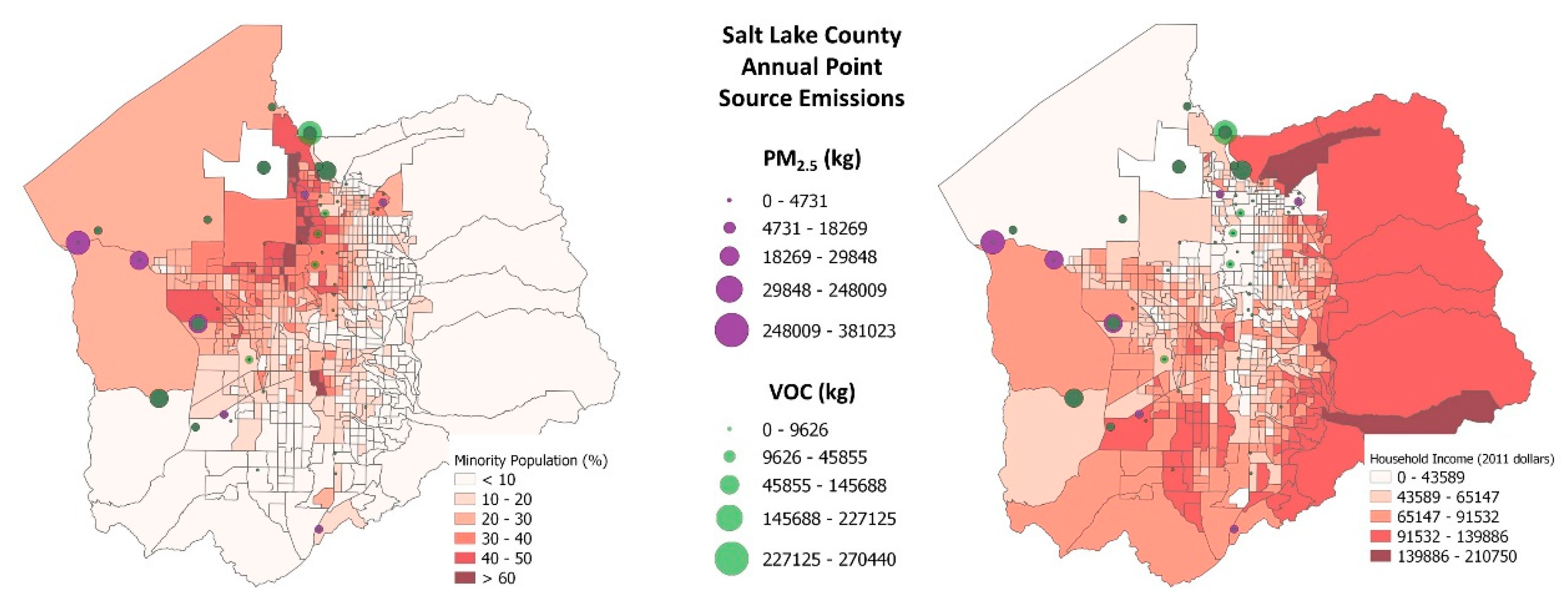
1.2.4. Sociodemographic and Emission Characteristics

The central and western sections of the SLV have a larger number of emission sources ranging from the airport, railroad tracks, industrial facilities, and major interstate and arterial roads [39,40]. Additionally, lower income and minority communities tend to be located along the central, and lower elevation, core of the valley (Figure 2). Figure 2 shows the distribution of point source emissions for PM2.5 and Volatile Organic Compounds (VOC), which are precursors to ozone formation, overlaid on sociodemographic maps of the SLV. Identifying the distribution of emission sources, in conjunction with monitoring the spatial distribution of pollutant exposure, is a necessary first step towards assessing potential health outcomes for vulnerable populations.

1.3. What this Adds to Previous Work

1.3.1. New Equipment on TRAX Trains and Quality Control and Quality Assurance of Data

The TRAX Observation Project started archiving data from its inception in December 2018, using a completely new suite of instruments to replace the sensors used in the Pilot Project. Significant efforts are being taken to perform appropriate quality control and quality assurance (QA/QC) checks on the data. These processes will increase the reliability of the observational data so that it can be used with greater confidence for diverse applications.

1.3.2. Public Awareness via Web Interface

An important contribution of the TRAX Observation Project is the real-time data availability through the website: https://atmos.utah.edu/air_quality/trax/. Time histories of the observations are available for user-selectable time periods, from an hour to several days. These web resources can be particularly useful for localized events (such as fireworks) or events that are geographically constrained (such as winter cold-air pools or dust events). They can also help inform whether it is recommended to reduce recreating outdoors. These web services are intended as a general reference, as specific locations may have different air quality, due to proximal sources of pollution. This website also provides information on data quality control, where and how to request access to the data, and other aspects of the study. This webpage will be continually updated over the coming years as the project expands and the data services evolve.

1.3.3. Support of Air Quality Initiatives by Policymakers and Health Agencies

As the project evolves, findings will be used to help inform and support air quality related efforts for both policymakers and health agencies. The first year (from July 2018 to June 2019) was dedicated to the testing and installation of sensors that are mounted on train cars that travel on the TRAX Red and Green lines (Figure 1). Sensors have been added during the second year to a third train car that traverses the TRAX Blue line, which will increase the coverage north–south through the core of the SLV and expand into the southeastern part of the SLV for the first time. The second year is also being dedicated to developing automated QA/QC approaches to process the raw observational data into a final product suited for health and policy applications.
The rest of the manuscript is structured as follows: Section 2 describes the equipment and methods used for the study, Section 3 presents the results, Section 4 provides the discussion of relevant findings, and Section 5 highlights the conclusions and future directions of this work.

2. Materials and Methods

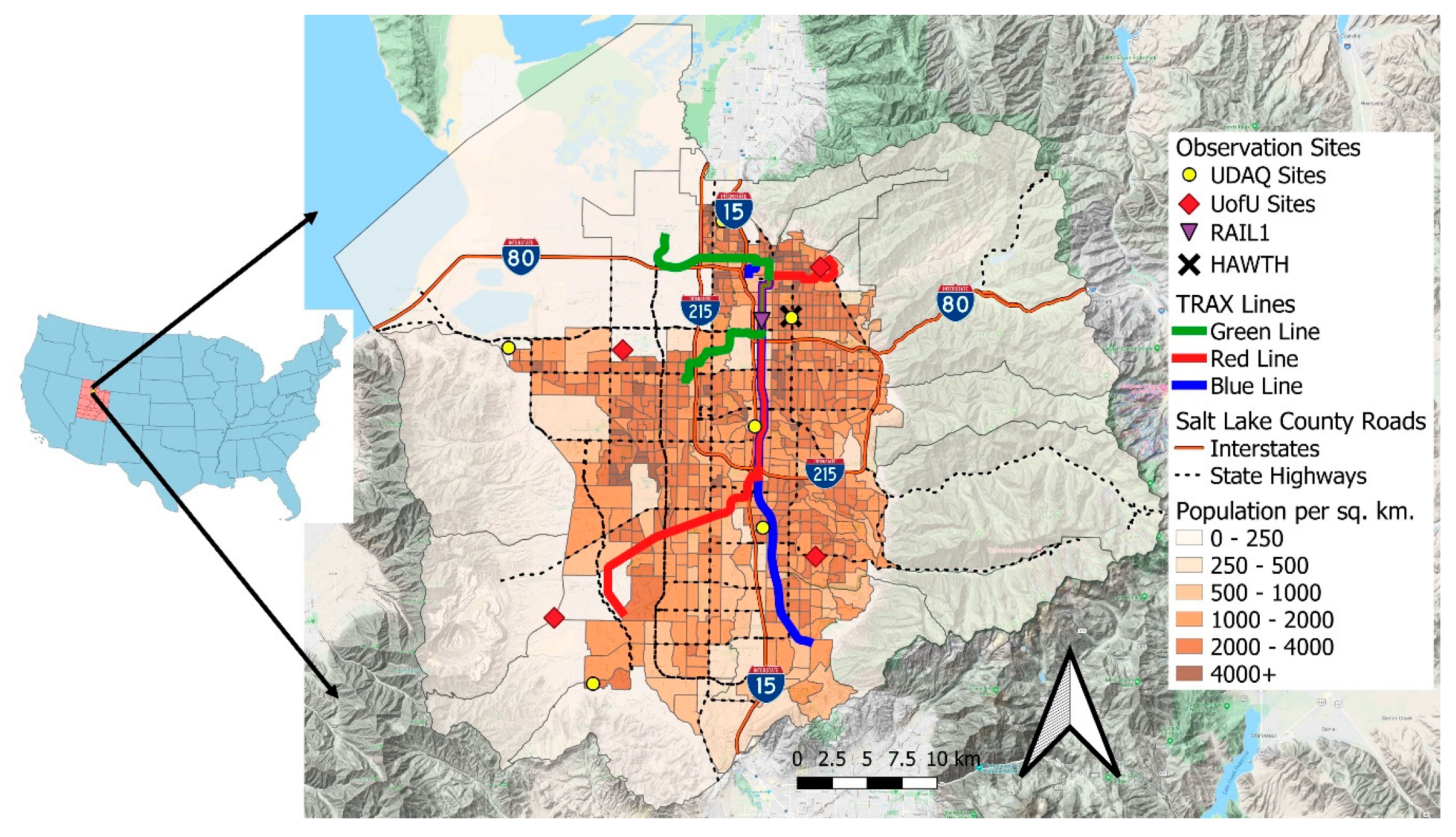
2.1. Location and Equipment

Two light-rail train cars, traveling on the Red and Green UTA TRAX lines, were outfitted with research-grade Met One Instruments ES-642 particulate sensors (with inlet sharp cut cyclone used for selective measurement of PM2.5) and EPA Federal Equivalent Method (FEM) 2B Technologies Model 205 Ozone Monitor sensors during November and December 2018. One train car traveling on the Blue TRAX line was outfitted with the same suite of equipment in November 2019. Inlets to the sensors are mounted 0.5 m above the top of the train with the sensors inside or attached to a metal box located four meters above the ground in an identical manner to the pilot study [7]. Fans were installed within the box in the summertime to avoid overheating of the instruments.
Two additional ES-642 PM2.5 sensors were sited at fixed ground sites to a) provide high-quality calibration match-up data with FEM PM2.5 sensors and b) to evaluate any potential impact of train motion on the PM2.5 observations. The first fixed ground site sensor (HAWTH) was co-located with a regulatory-grade FEM sensor at a UDAQ site (HW) to compare with their PM2.5 readings. The second sensor (RAIL1) was placed on a UTA service shed located approximately three meters from the rail line at a location where inlet effects might be a factor, since the trains are typically moving at 85 km/h in that location. The FEM ozone sensors are not subject to the train motion and inlet effects, and thus no ground validation sites were needed for ozone, as ground-based stationary [41], ground-based mobile [3], and aircraft-based campaigns have used this sensor [42]. These sensors were maintained and calibrated monthly to ensure accurate ozone data collection. The locations of the fixed site sensors, as well as the various light rail routes, are shown in Figure 1. The location, purpose, instrument type, and installation date are shown in Table 1.

2.2. Data Recorded

The raw data from the mobile and stationary criteria pollutant sensors are collected at 2-second intervals and recorded fields include time, temperature (°C), relative humidity (%), pollutant concentration (µg m−3 for PM2.5 and parts per billion, ppb, for ozone), and GPS location. The TRAX light rail train network consists of approximately 150 electric trains services and ~100 km of track across the SLV. The frequency of the trains varies considerably, with most trains in operation during busy periods and only a few trains running on operational holidays (the train runs year-round except on New Year’s Day and Christmas). On average, TRAX trains run ~60% of the time [7]. There are 25, 19, and 19 passenger stops along the Red, Blue, and Green Line, respectively, and train arrival frequency (separation between trains) at any given station averages ~15 min. It takes between 42–60 min for a one-way transect by a train line along one of the three track segments. A train that is deployed on any given day averages 14 transects [7].
The research-grade instruments listed in Table 1 have the following uncertainties:
  • Met One Instruments ES-642→1 µg m−3 [43];
  • 2B Technologies Model 205 Ozone Monitor→2% [44].
Both research-grade and FEM nephelometers suffer from errors during high humidity conditions [45]. The impacts of humidity below 90% are largely mitigated by a heating element in the ES-642 sensors that is automatically turned on when the relative humidity exceeds 35%. However, when the ambient humidity is > 90%, which is common during fog events, the heating elements are unable to dry the air sufficiently and particles undergo hygroscopic swelling that can lead to a high bias in the ES-642 sensors. Periods of high relative humidity > 90% are therefore flagged with the option to remove accompanying particulate observations from later analyses. For this study, aerosol backscatter from a ceilometer located on the east side of the SLV was also used to help estimate the presence of low clouds or fog that would lead to inaccurate high values of PM2.5.

2.3. Quality Control/Quality Assurance

The RAIL1 and TRAX ES-642 sensors are equipped with a TSP (Total Suspended Particle) inlet and a PM2.5 sharp-cut cyclone from Met One and therefore do not have an isokinetic inlet. Therefore, the QA/QC process involved comparing observations from the stationary RAIL1 sensor with those from TRX01 and TRX02 as the trains passed RAIL1 to understand if turbulence and pressure effects from the movement of the train resulted in errors in the data readings. RAIL1 is located at the midpoint between two stations that are nearly two kilometers apart and the trains can reach their highest speed (~85 kph) at this point. The TRX01 and TRX02 2-second data were compared to 10-second RAIL1 data when the trains were within 150 meters from RAIL1. The last step of the QA/QC process was to compare HAWTH readings against those from the regulatory 1-hour UDAQ sensor (HW).
A significant concern of any observation campaign is the reliability of the measurements. While regulatory grade (FEM, or Federal Equivalent Method) air quality sensor equipment must have a dedicated team to maintain and parse through the data, other sensor networks follow less structured protocols. The TRAX Observation Project, due to its importance as the backbone of future health studies and policy applications, is subject to stringent QA/QC procedures. Instruments are physically examined, and flow checks and calibrations are conducted on a monthly basis by dedicated technicians who are tasked specifically with maintaining the equipment. A replacement set of tested and calibrated instrumentation is always available to replace any sensors that may need maintenance, avoiding the gaps in data coverage that impacted the pilot study. Furthermore, the TRAX Observation Project team, composed of faculty, staff, and students, are subscribed to an alert system that sends an email to the entire team when the instrument diagnostic data (e.g., flow rate, battery voltage) is outside specified ranges. This permits a quick response if something can be fixed remotely, or schedules repairs as soon as possible, in order to foster high levels of reliability and instrument uptime.

3. Results

3.1. Quality Assurance/Quality Control Results

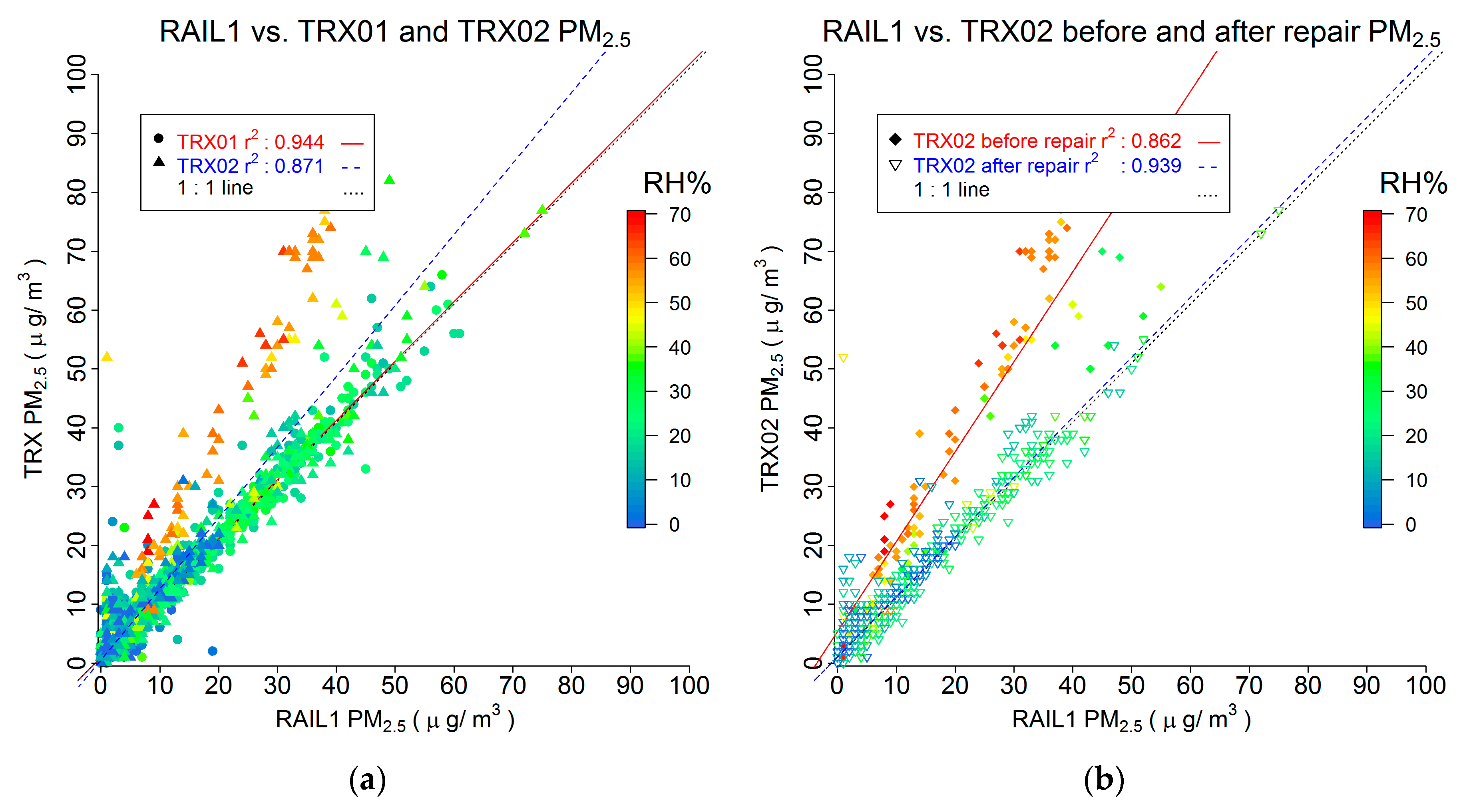
3.1.1. TRAX-Mounted Sensor Comparison with RAIL1 Stationary Site

Data from the RAIL1 stationary sensor are compared to those from the mobile sensors (TRX01 and TRX02) for the times when the light rail cars are near the RAIL1 site, from December 2018 until July 2019 (Figure 3). The RAIL1 and TRX01 and 02 sensors are strongly correlated, which suggests limited inlet effects (Figure 3a). The high degree of correlation between the TRX01 and 02 and RAIL1 observations, in addition to no observable bias when compared to the 1:1 line, suggests that the speed of the traveling train cars has no observable effect on PM2.5 concentrations. It became apparent after the first 10 days after installation that the relative humidity sensor in TRX02 was malfunctioning and was failing to trigger the heater to turn on when the relative humidity exceeded 35%, leading to some data having elevated relative humidity values (Figure 3a). After the sensor was repaired, the variations in RAIL1 and TRX02 were similar (Figure 3b).

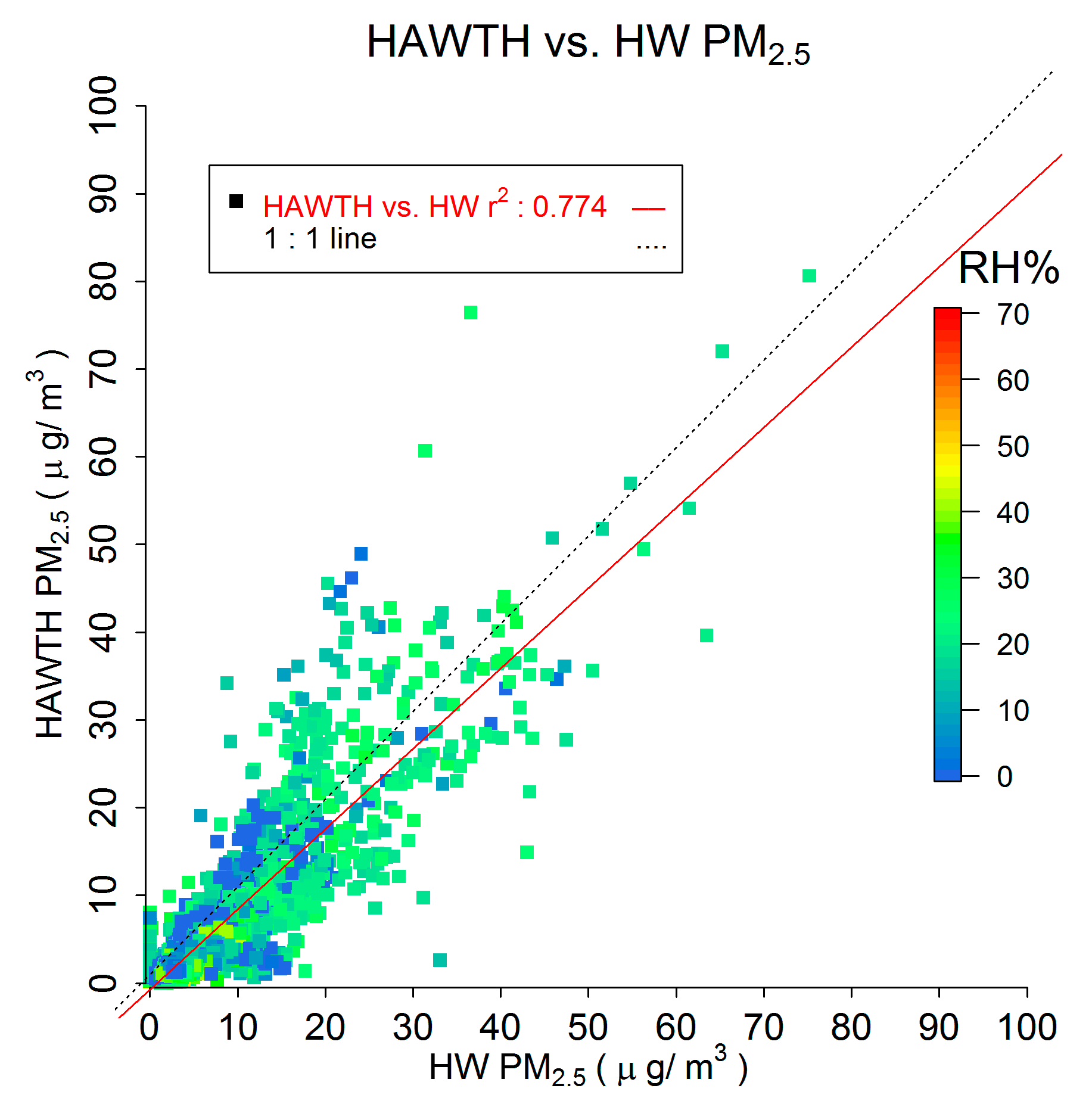
3.1.2. Comparison with HW Regulatory Site

The comparison of the HAWTH stationary sensor to the FEM sensor (HW) is shown in Figure 4. There is generally good agreement between HAWTH and HW. Discrepancies are to be expected, given the different measurement technologies used. For example, the air entering the HW FEM sensor is heated to a high temperature (50 °C) in order to measure dry particulate mass, while HAWTH only heats the air enough to maintain a low relative humidity (35% or lower).

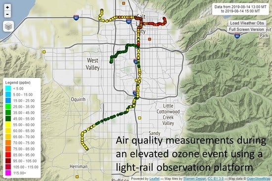
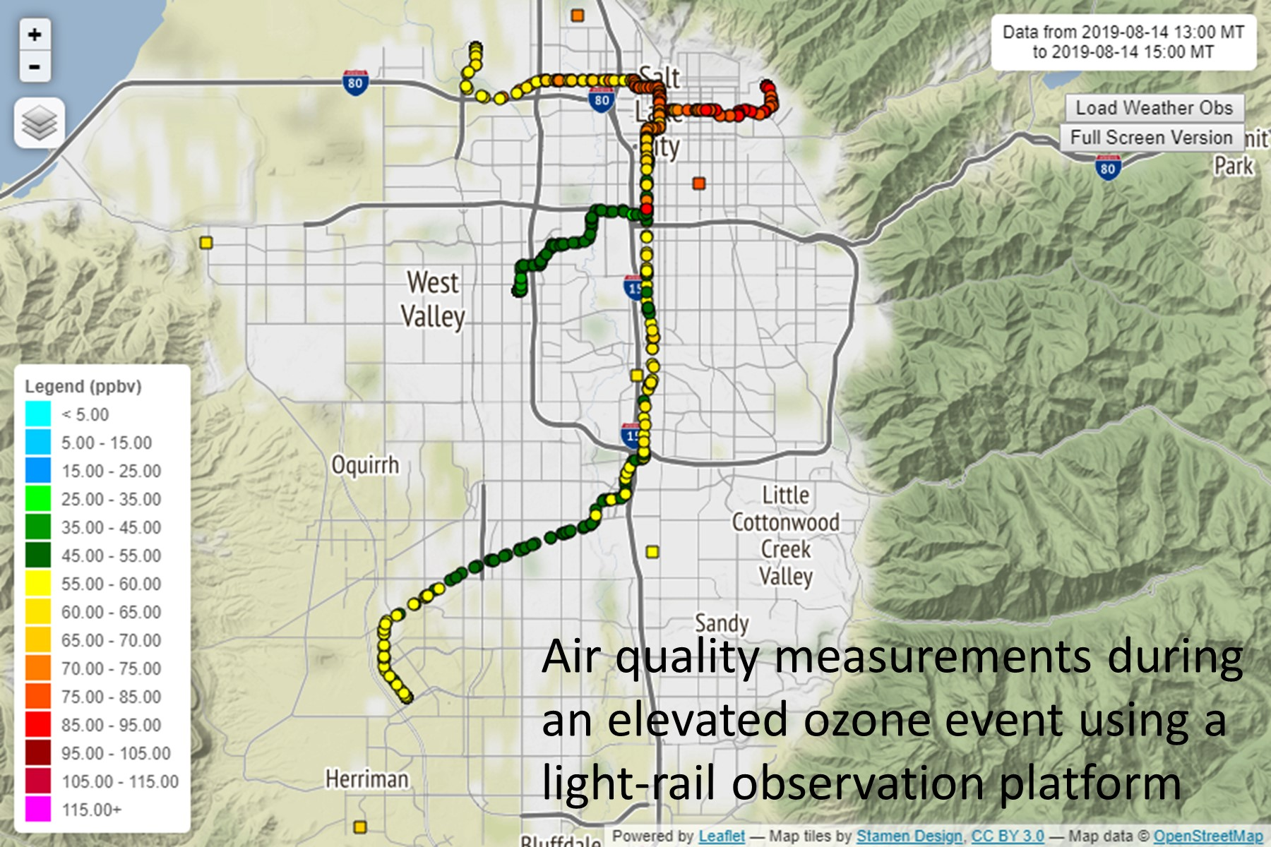
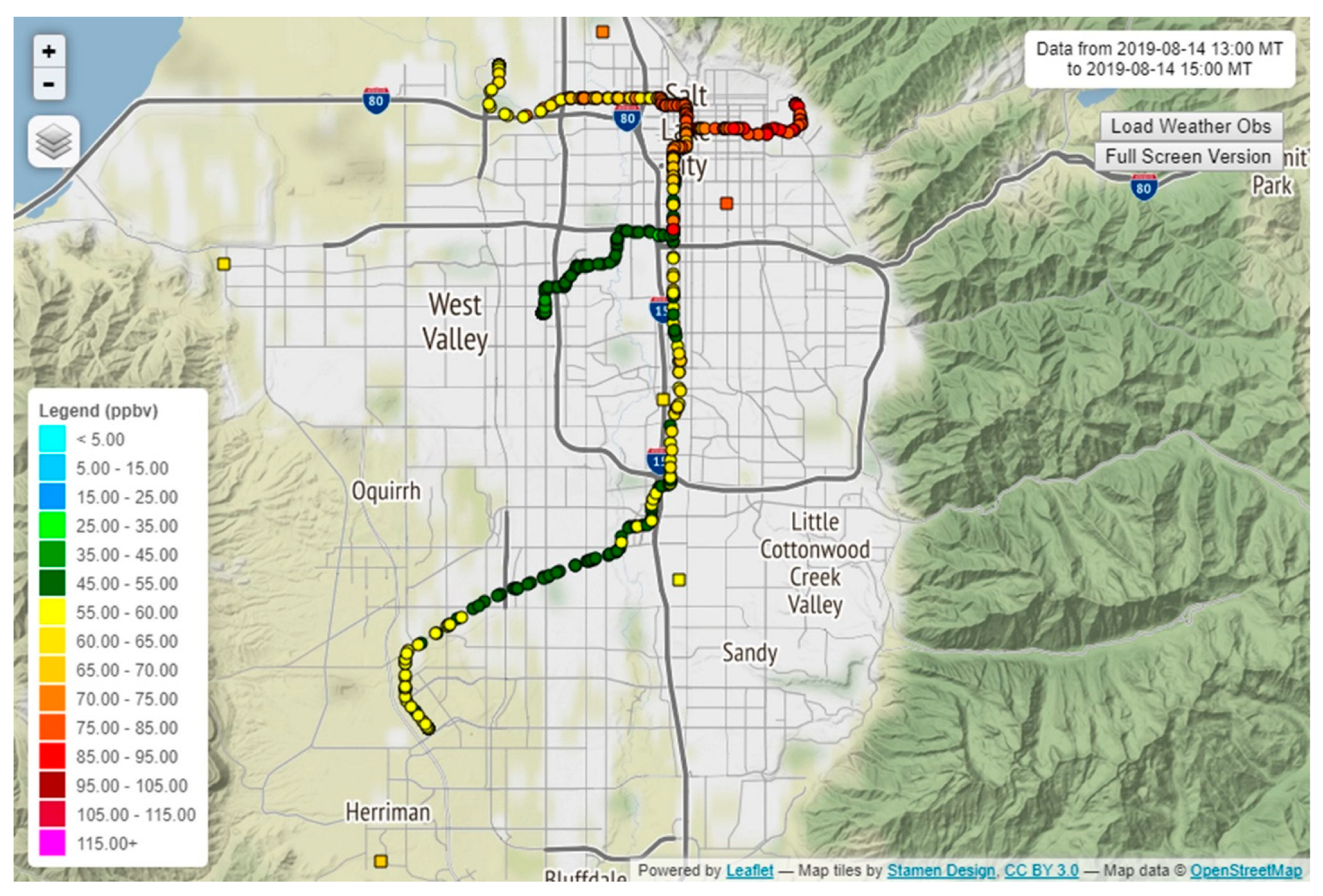
3.2. Elevated Ozone Case Study: August 8th, 2019

An elevated ozone event took place on August 8th, 2019. During the afternoon, ozone levels ranged from “good” to “unhealthy”, with most of the SLV experiencing “unhealthy for sensitive groups” and “moderate” air quality index (AQI) readings [46]. This ozone event was one of more than a dozen days where the AQI “unhealthy” levels were reached during the summer of 2019.
The ozone measurements over a 2-h time frame, from 13:00–15:00 Mountain Daylight Savings Time (MDT) on August 8th, 2019, from the TRAX Observation Project website, are shown in Figure 5. Ozone levels range from “good” in the lower elevation parts of the SLV to “unhealthy” in the outer parts of the SLV. It is well-understood that ozone distribution, particularly in areas with complex topography, is heterogeneous, in addition to spatial differences in NOx titration rates coupled with wind patterns.

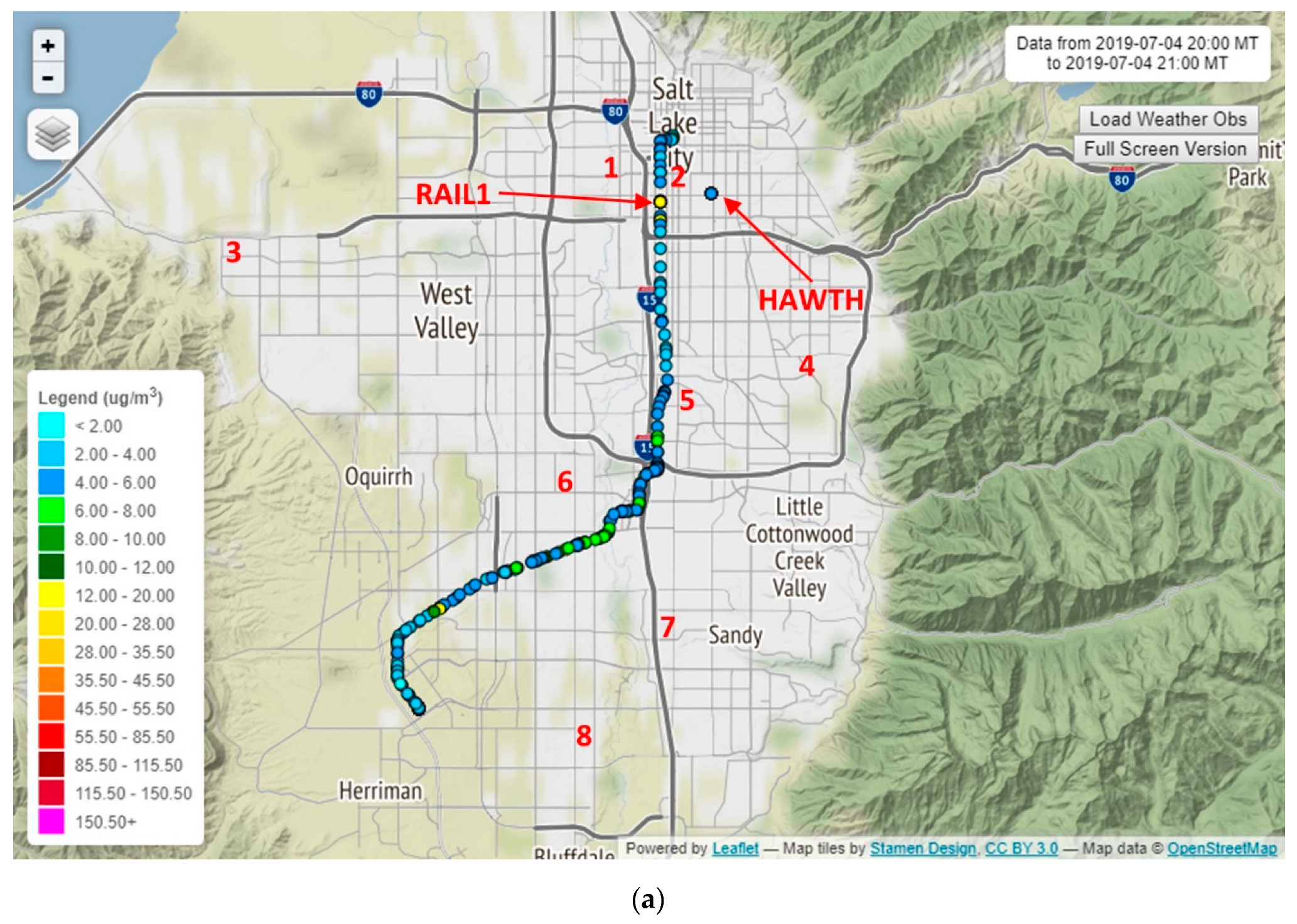
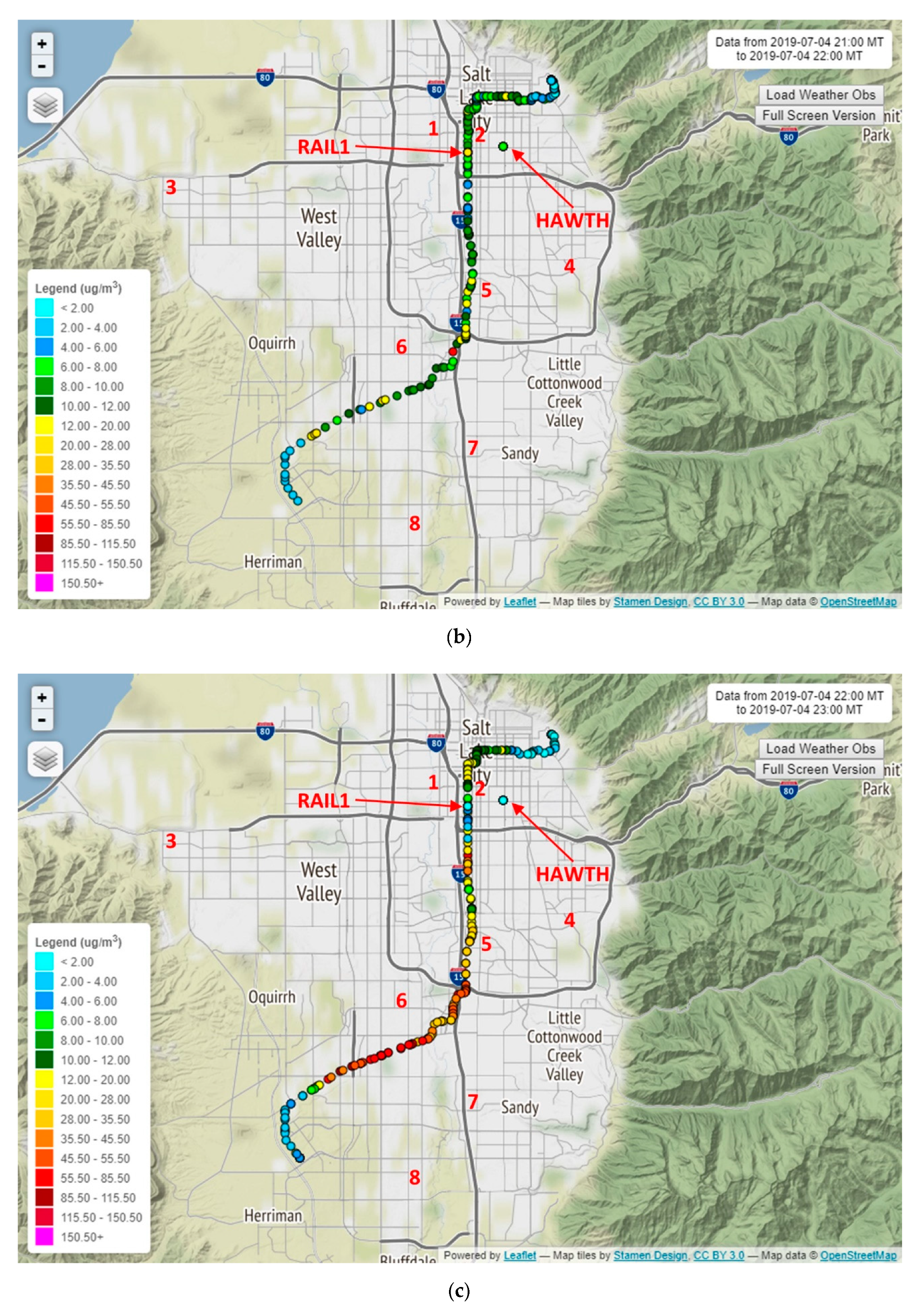
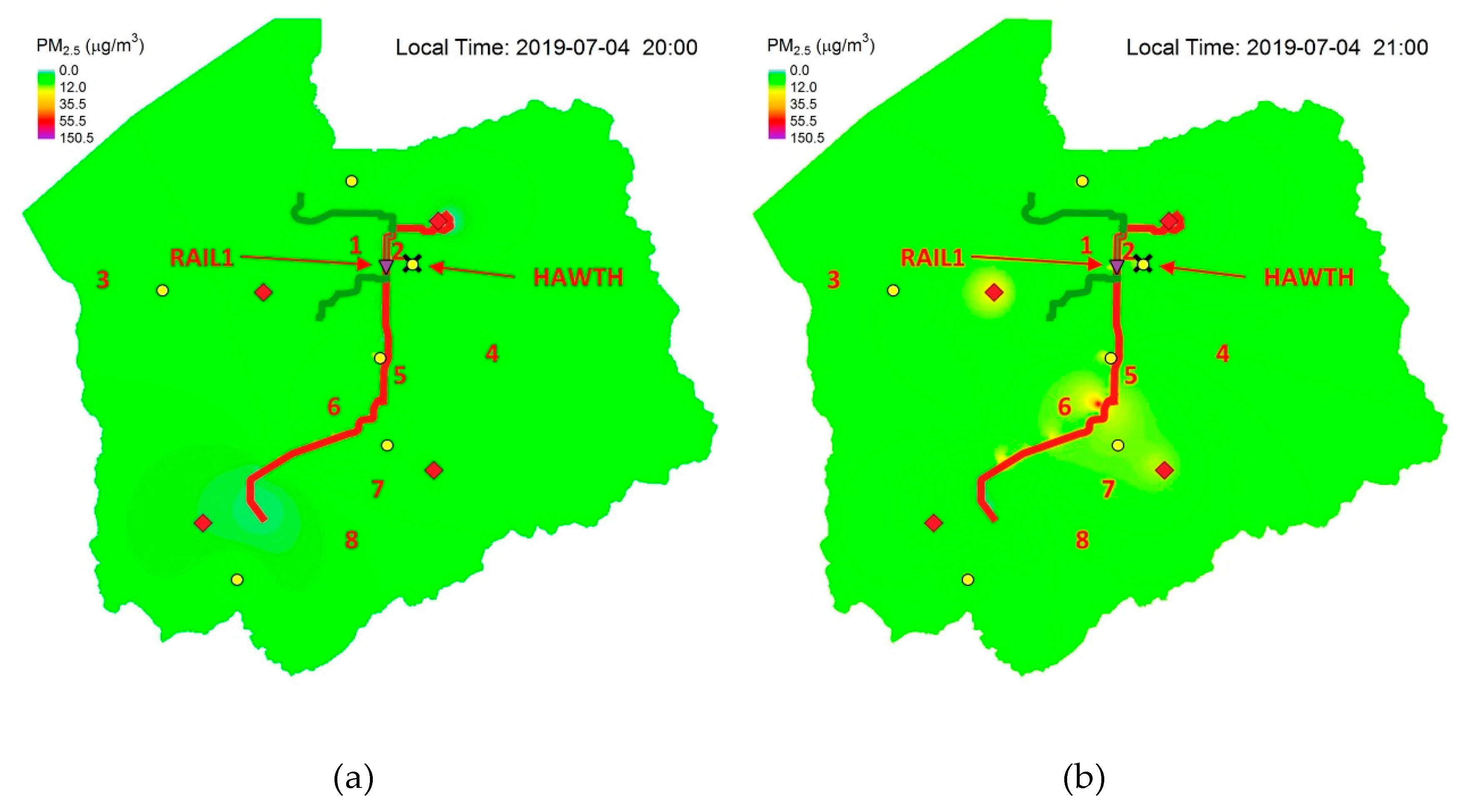
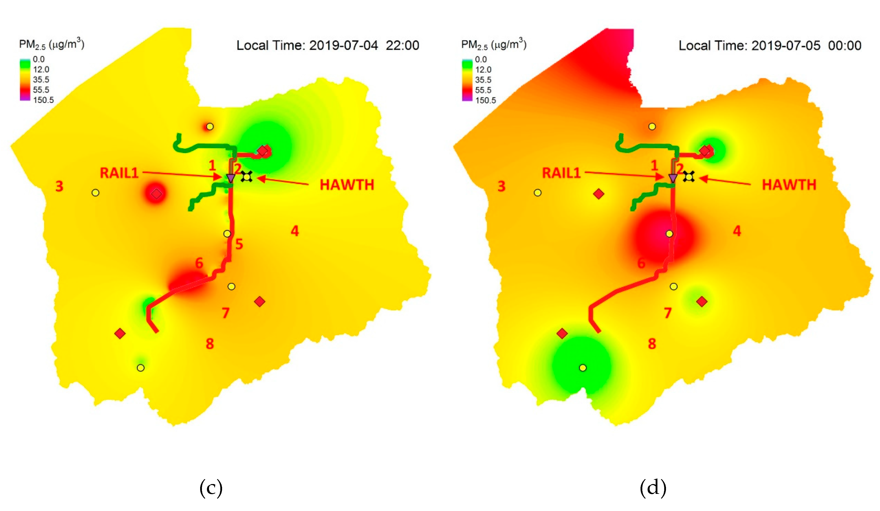
3.3. Elevated PM2.5 Case Study: July 4th, 2019 Fireworks

The July 4th national holiday in the United States (Independence Day) is usually accompanied by multiple firework displays across communities [47]. The SLV had seven locations where large public fireworks shows were launched during July 4th, 2019 (Table 2). Firework shows are known to lead to localized and rapid increases in particulate concentrations nearby [48]. Large firework events, including those associated with the Diwali celebrations in India [49], religious festivals in Malta [50], and the Spring Festival in China [51], have consistently shown the deterioration in air quality associated with fireworks. During the 4th of July holiday, most of the SLV sites started their fireworks shows at 22:00 MDT, with the exception of the Veteran’s Memorial Park (Site 6 in Figure 6), which started at 22:15 MDT, and Smith’s Ballpark (Site 2 in Figure 6), which started at approximately 22:45 MDT at the conclusion of a baseball game.
The July 4th holiday PM2.5 observations from TRAX are shown in Figure 6, with spatially interpolated PM2.5 estimates using inverse distance weighting [52] presented in Figure 7. Before the fireworks began (20:00–20:59 MDT, Figure 6a), the PM2.5 concentrations are low throughout the SLV, with the exception of the reading at RAIL1. As these are min-resolved readings, the last min on the stationary RAIL1 site is from 20:59 MDT, and the elevated value may be due to either an isolated firework or a passing vehicle. Although the fireworks were getting ready to start at 10:00 PM MDT, Figure 6b shows slightly elevated concentrations in the 21:00–22:00 MDT time frame near some of the large roads, which could be due to vehicular traffic. Between 22:00-23:00 MDT (Figure 6c), hotspots near the firework locations were visibly apparent in some areas, particularly in the southwest part of the county where conditions reached “unhealthy” air quality levels. At the 23:00–00:00 MDT timeframe (Figure 6d), the majority of the study area observed air quality that ranged from “moderate” to “unhealthy”, with the exception of the southwestern corner of the Salt Lake Valley. This area is at a higher elevation than the rest of the valley and did not have nearby firework particulate emission sites.
Figure 7 mirrors the timeframes used in Figure 6. The data from TRX01, TRX02, HAWTH, and RAIL1 were included in the modeling approach and regulatory readings from UDAQ, as well as from other research-grade sensors operated by the University of Utah, were also used (Figure 1). The hotpots and dispersion effects are apparent throughout the episode evolution between 21:00–22:00 MDT. As with any inverse distance weighing method, care must be taken when interpreting values farther away from observations. A benefit of the TRAX platform is that the rail lines are located along the most densely populated areas, while the outer edges of the county are primarily composed of mountains or wetlands and the Great Salt Lake.

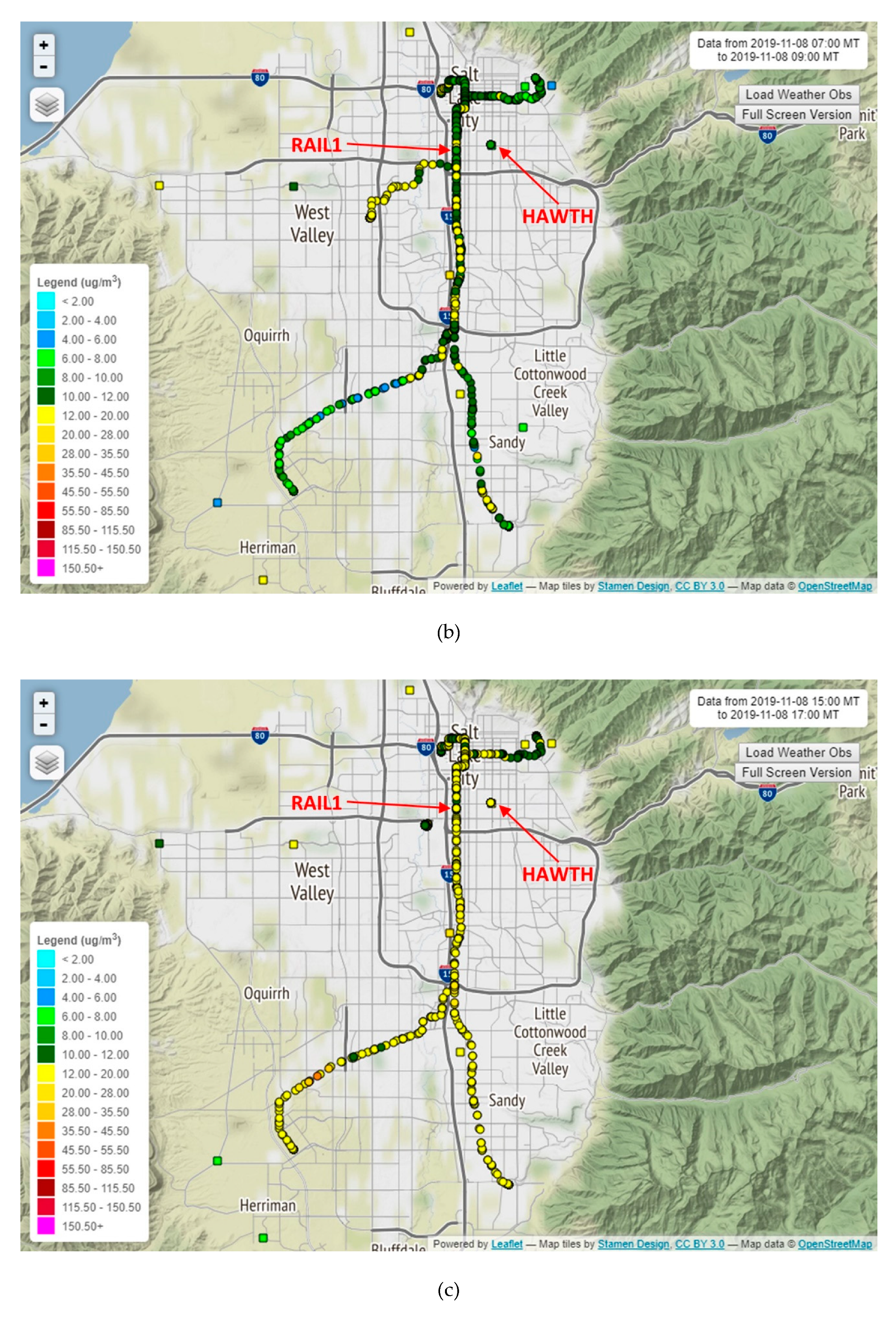
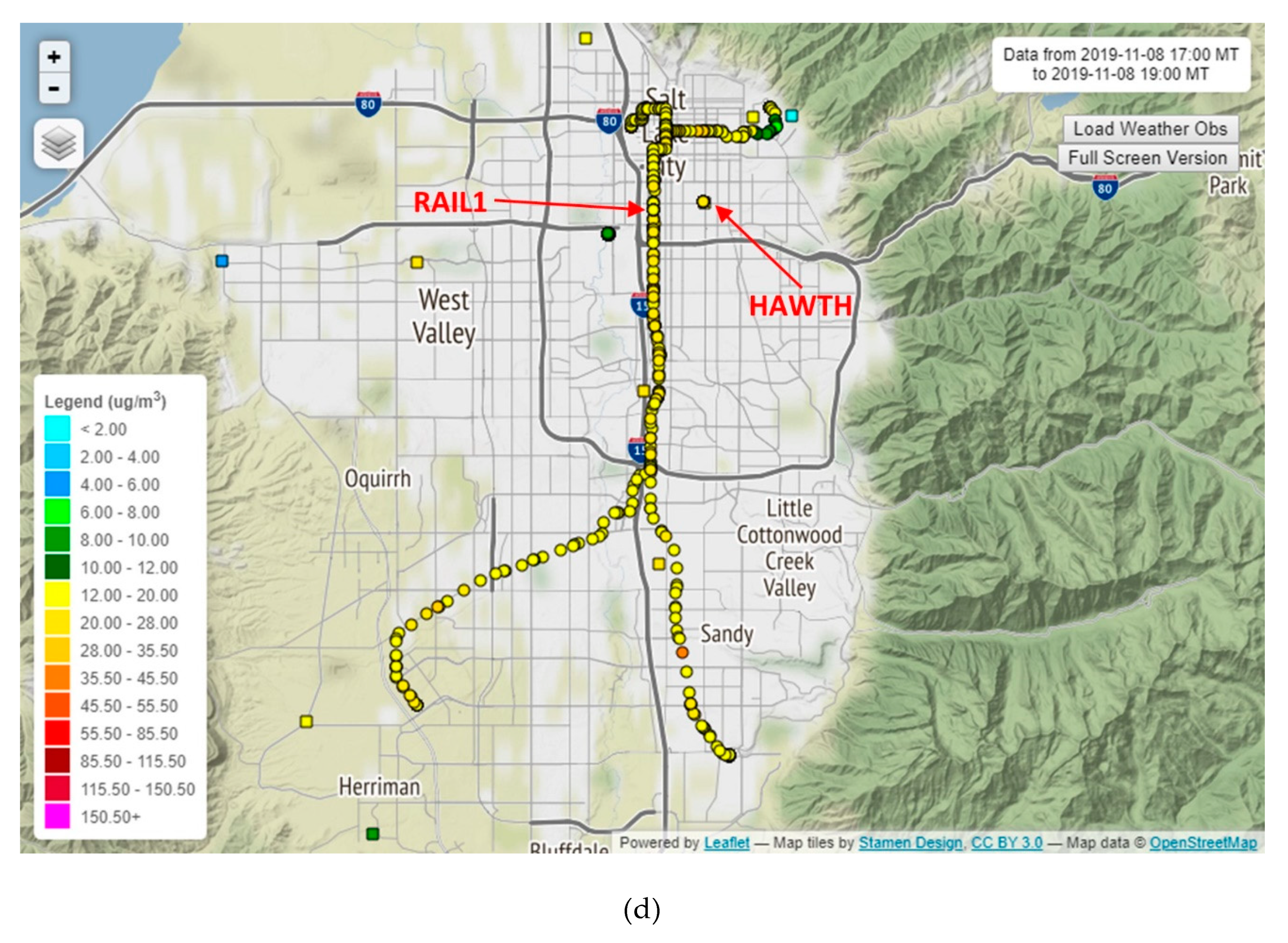
3.4. Elevated PM2.5 Case Study: November 8th, 2019

A cold air pool event on November 8th, 2019 led to elevated PM2.5 levels throughout the SLV (Figure 8). During the afternoon, PM2.5 levels ranged from “good” to “moderate” with a few instances of “unhealthy for sensitive groups” AQI readings [46]. This event was the first recorded since the installation of TRX03 and shows the air quality of the southeast part of the SLV (Blue line) in addition to the other parts of the SLV covered by the Red and Green lines.
The PM2.5 measurements over a 2-h time frame, primarily centered on peak traffic hours from the TRAX Observation Project website, are shown in Figure 9. During the early morning hours (05:00–07:00 MST) the air quality is primarily “good” throughout the entire SLV, with the exception of the southern intersection of Interstates 15 and 215 (Figure 9a). During and after the morning rush hour (07:00–09:00 MST) areas around the interstate highways and the lower elevation parts of the SLV show degraded air quality conditions (Figure 9b). By the early afternoon hours (15:00–17:00 MST) the majority of the SLV shows “moderate” air quality conditions, with the exception of the higher elevation areas in the northeastern parts (Figure 9c). Clean inflow from several topographic canyons are injecting lower pollution into the SLV at these locations, as discussed in the pilot project [7]. Following the afternoon rush hour (17:00–19:00 MST) the entirety of the SLV shows “moderate” air quality conditions, except for the highest observation point in the foothills in the northeast quadrant of the SLV and toward the Great Salt Lake, due to cleaner air masses resulting from the aforementioned canyon flows and also potentially from Great Salt Lake Breezes at the westernmost site.

4. Discussion

4.1. Quality Control and Quality Assurance

A critical, but understudied, question was the potential impact of the movement of the train on PM2.5 readings. The comparison of TRAX mounted sensor readings against stationary readings from RAIL1 showed that there is little to no effect of train motion on observational data using our experimental setup. The comparison of HAWTH against the HW regulatory sensor showed close agreement and further strengthens the significance of the TRAX Observation Projection as a reliable complement to regulatory and research grade stationary sensor networks.

4.2. Ozone Events

The ozone event shown in Figure 5 follows two expected patterns found in previous studies; ozone concentrations are generally higher in higher elevation areas and lowest near large roads with high vehicular traffic due to NOx titration effects. Ozone is a particularly dangerous pollutant because, unlike particulate matter, it is invisible, and therefore people do not take precautionary measures to reduce their exposure during high ozone events. As ozone is generally elevated during the summer months, when people exercise outside more often, and children are on school vacation, fine-scale monitoring efforts are important to help inform the public of potentially hazardous conditions. The TRAX Observation Project has shown how light-rail based mobile measurements can be used to reliably show highly resolved ozone gradients in the Salt Lake Valley (SLV) region. As warming temperature trends have been the norm for the past decades and ozone photochemical reactions occur more rapidly in warmer conditions, ozone is expected to become a larger concern in the near future.

4.3. PM2.5 Events

The July 4th holiday has the largest number and intensity of firework displays in the Salt Lake County region. Many of these events occur in parks and other large and well-ventilated areas. However, the Smith’s Ballpark fireworks take place near the stadium. The capacity of the ballpark is over 14,500 people and these games are generally well-attended. With limited air flow, due to the shape of the stadium, pollutant accumulation is a significant concern in this venue. Being able to provide an estimate of potential exposure and associated health effects may help start the conversation to reduce the number and intensity of firework events, particularly in confined areas with large amounts of people. Data from the TRAX Observation Project can also identify the most vulnerable areas to not only exceptional events (such as fireworks and dust storms), but also areas that are chronically affected by elevated PM2.5. This can help inform urban planning efforts designed to mitigate emissions, as models can be developed and validated by observations. A significant benefit of the data obtained from the TRAX Observation Project is that, through our analysis and QA/QC procedures, we are assured of the high quality of the resultant data. The research grade sensors used on the TRAX Observation Project are robust across a broader environmental range than low-cost sensor networks, thus the data can be reliably used for health and policy purposes.
The November 8th inversion event was the first for the 2019–2020 winter season in the SLV, and the addition of sensors on the Blue line the week before will now allow for unprecedented observation capabilities for the southeaster SLV going into the 2020 winter season. The broader coverage showed that the higher elevation southwest part of the SLV generally had cleaner air than the more populated and lower elevation southeast part, and the valley-wide impact of traffic rush hours and canyon flows and lake breezes from the Great Salt Lake on air quality. The southernmost end of the Blue line observations is relatively close to the Jordan Narrow gap that separates the SLV and Utah Valleys, thus this new observation capability will now observe this inter-basin exchange process.

5. Conclusions

5.1. Implications

The TRAX Observation Project provides a research-grade dense observation network that allows fine-scale PM2.5 and ozone exposure estimates to be made and exposure models developed. In conjunction with additional UDAQ and University of Utah regulatory and research grade instruments, the TRAX Observation Project can be used to inform health studies with reliable data to advance granular research linking air exposure and health outcomes at neighborhood scales. Socioeconomically disadvantaged and vulnerable populations tend to face larger environmental challenges due to generally living in closer proximity to air pollution sources. The ability to quantify and characterize possible health hazards at finer scales is a significant advantage when developing potential policy measures to protect vulnerable populations. The long-term nature of this project will also facilitate analysis of the impact of emission reduction strategies and help evaluate their potential health and societal benefits. The regular TRAX schedule also ensures that repeated observations provide sufficient high-quality data for long-term trend analyses.

5.2. Limitations

An important limitation of the study is that the TRAX observations must be considered as representing only the temporal resolution at a particular spatial location. This is most apparent during brief episodes such as the fireworks event (Figure 6 and Figure 7). During the 10:00–11:00 PM MDT timeframe (Figure 6c), the TRAX trains were not near the Jordan Park or Smith’s Ballpark fireworks site, thus, the PM2.5 signal was not present in that figure or in Figure 7c. Between 11:00 PM–12:00 AM MDT (Figure 6d and Figure 7d), the TRAX trains pass near those fireworks locations and the residual PM2.5 is recorded, but the immediate hotpots from those two events are missed. Therefore, care must be taken when using this data to represent spatially explicit air quality, particularly at longer time scales, due to potential scheduling limitations of TRAX trains.

5.3. Future Work

The Blue Line TRAX train (Figure 1) was instrumented on November 4th, 2019. This additional train will provide information on the southeastern part of the SLV and reach almost to the border, with Utah County in the south. The Traverse Mountains, between the SLV and Utah County, form an elevated narrow passage where air masses can travel between the two counties, and the Blue Line TRAX should be able to capture the signal of this air and pollutant exchange.
Several health-related studies are currently underway utilizing the TRAX data to more finely disaggregate pollutant exposure in populations across the SLV. Findings from the TRAX Observation Project have shown that pollutant (both PM2.5 and ozone) concentrations vary widely, even across relatively small areas. This information will be used to support emissions mitigation strategy proposals, both from a legislative and planning perspective. Additionally, these findings can support requests for fixed observation sites in areas of specific concern where pollutants have been found to be elevated or a large number of vulnerable individuals live, particularly near large emitting sources.

Author Contributions

Conceptualization, A.A.J., B.F., D.L.M., E.T.C., J.D.H., J.C.L., and L.E.M.; methodology, D.L.M. and E.T.C.; software, A.A.J., D.L.M., and E.T.C.; validation, A.A.J., A.M.P., B.F., D.L.M., E.T.C., J.D.H., J.C.L., and L.E.M.; formal analysis, D.L.M. and E.T.C.; investigation, A.A.J., B.F., D.L.M., E.T.C., J.D.H., J.C.L., and L.E.M.; resources, A.A.J., B.F., D.L.M., E.T.C., J.D.H., J.C.L., and L.E.M.; data curation, A.A.J., D.L.M., and E.T.C.; writing—original draft preparation, D.L.M.; writing—review and editing, A.A.J., A.M.P., B.F., D.L.M., E.T.C., J.D.H., J.C.L., and L.E.M.; visualization, A.A.J., D.L.M., and E.T.C.; supervision, D.M. and E.T.C.; project administration, D.L.M. and E.T.C.; funding acquisition, D.L.M.

Funding

This research was funded by: The Utah Division of Air Quality.

Acknowledgments

In-kind contribution of technician and organizational time was provided by the Utah Transit Authority. The authors are grateful to the Utah Transit Authority (UTA) for supporting the installation of air quality sensors on their light rail trains. Special thanks go to James (Tal) Brooks, Teresa Jessen, Dan Christenson, William Patterson, and Elijah Jackson at UTA for assistance with the equipment installation and ongoing access to the trains for maintenance. Thanks also goes to Bo Call, Luke-Leclair Marzolf, Katie Chachere, and the Utah Division of Air Quality for allowing for validation sites to be co-located at Hawthorne Elementary state of Utah regulatory air quality site, and for their help with installation. We also thank the Center for High Performance Computing at the University of Utah for their support and resources. The authors thank the editors and reviewers.

Conflicts of Interest

The authors declare no conflict of interest. The funders had no role in the design of the study; in the collection, analyses, or interpretation of data; in the writing of the manuscript, or in the decision to publish the results.

Abbreviations

The following abbreviations are used in the manuscript:
CH4Methane
CO2Carbon dioxide
EPAEnvironmental Protection Agency
NAAQSNational Ambient Air Quality Standards
NO2Nitrogen dioxide
NOxNitrogen oxides
O3Ozone
PM2.5Fine particulate matter
QAQuality Assurance
QCQuality Control
SLCSalt Lake City
SLVSalt Lake Valley
TRAXTransit Express
UofUUniversity of Utah
UDAQUtah Division of Air Quality
UTAUtah Transit Authority

References

  1. Kem, C.; Gardner Policy Institute. Utah’s Long-Term Demographic and Economic Projections; Gardner Policy Institute: Salt Lake City, UT, USA, 2017. [Google Scholar]
  2. Lareau, N.P.; Crosman, E.; Whiteman, C.D.; Horel, J.D.; Hoch, S.W.; Brown, W.O.J.; Horst, T.W. The Persistent Cold-Air Pool Study. Bull. Am. Meteorol. Soc. 2012, 94, 51–63. [Google Scholar] [CrossRef]
  3. Horel, J.; Crosman, E.; Jacques, A.; Blaylock, B.; Arens, S.; Long, A.; Sohl, J.; Martin, R. Summer ozone concentrations in the vicinity of the Great Salt Lake. Atmos. Sci. Lett. 2016, 17, 480–486. [Google Scholar] [CrossRef]
  4. Crosman, E.T.; Horel, J.D. Winter lake breezes near the Great Salt Lake. Bound.-Layer Meteorol. 2016, 159, 439–464. [Google Scholar] [CrossRef]
  5. Baasandorj, M.; Hoch, S.W.; Bares, R.; Lin, J.C.; Brown, S.S.; Millet, D.B.; Martin, R.; Kelly, K.; Zarzana, K.J.; Whiteman, C.D.; et al. Coupling between Chemical and Meteorological Processes under Persistent Cold-Air Pool Conditions: Evolution of Wintertime PM2.5 Pollution Events and N2O5 Observations in Utah’s Salt Lake Valley. Environ. Sci. Technol. 2017, 51, 5941–5950. [Google Scholar] [CrossRef]
  6. Whiteman, C.D.; Hoch, S.W.; Horel, J.D.; Charland, A. Relationship between particulate air pollution and meteorological variables in Utah’s Salt Lake Valley. Atmos. Environ. 2014, 94, 742–753. [Google Scholar] [CrossRef]
  7. Mitchell, L.E.; Crosman, E.T.; Jacques, A.A.; Fasoli, B.; Leclair-Marzolf, L.; Horel, J.; Bowling, D.R.; Ehleringer, J.R.; Lin, J.C. Monitoring of greenhouse gases and pollutants across an urban area using a light-rail public transit platform. Atmos. Environ. 2018, 187, 9–23. [Google Scholar] [CrossRef]
  8. Blaylock, B.K.; Horel, J.D.; Crosman, E.T. Impact of Lake Breezes on Summer Ozone Concentrations in the Salt Lake Valley. J. Appl. Meteorol. Climatol. 2017, 56, 353–370. [Google Scholar] [CrossRef]
  9. Wasatch Front Regional Council. Regional Transportation Plan 2015–2040; Wasatch Front Regional Council: Salt Lake City, UT, USA, 2015. [Google Scholar]
  10. Wasatch Front Regional Council. Wasatch Choice for 2040 Vision 2011–2040 Regional Transportation Plan; Wasatch Front Regional Council: Salt Lake City, UT, USA, 2011. [Google Scholar]
  11. American Lung Association. State of the Air 2018; American Lung Association: Chicago, IL, USA, 2018. [Google Scholar]
  12. Utah Department of Environmental Quality. Utah Division of Air Quality 2017 Annual Report; Utah Department of Environmental Quality: Salt Lake City, UT, USA, 2017. [Google Scholar]
  13. Pirozzi, C.S.; Jones, B.E.; VanDerslice, J.A.; Zhang, Y.; Paine, R., III; Dean, N.C. Short-Term Air Pollution and Incident Pneumonia. A Case–Crossover Study. Ann. Am. Thorac. Soc. 2018, 15, 449–459. [Google Scholar] [CrossRef]
  14. Horne, B.D.; Joy, E.A.; Hofmann, M.G.; Gesteland, P.H.; Cannon, J.B.; Lefler, J.S.; Blagev, D.P.; Korgenski, E.K.; Torosyan, N.; Hansen, G.I. Short-term elevation of fine particulate matter air pollution and acute lower respiratory infection. Am. J. Respir. Crit. Care Med. 2018, 198, 759–766. [Google Scholar] [CrossRef]
  15. Pope, C.A., 3rd; Renlund, D.G.; Kfoury, A.G.; May, H.T.; Horne, B.D. Relation of heart failure hospitalization to exposure to fine particulate air pollution. Am. J. Cardiol. 2008, 102, 1230–1234. [Google Scholar] [CrossRef]
  16. Pope, C.A., 3rd; Muhlestein, J.B.; May, H.T.; Renlund, D.G.; Anderson, J.L.; Horne, B.D. Ischemic heart disease events triggered by short-term exposure to fine particulate air pollution. Circulation 2006, 114, 2443–2448. [Google Scholar] [CrossRef] [PubMed]
  17. Hackmann, D.; Sjöberg, E. Ambient air pollution and pregnancy outcomes—A study of functional form and policy implications. Air Qual. Atmos. Health 2016, 10, 129–137. [Google Scholar] [CrossRef]
  18. Hales, N.M.; Barton, C.C.; Ransom, M.R.; Allen, R.T.; Pope, C.A., 3rd. A Quasi-Experimental Analysis of Elementary School Absences and Fine Particulate Air Pollution. Medicine 2016, 95, e2916. [Google Scholar] [CrossRef] [PubMed]
  19. Bares, R.; Lin, J.C.; Hoch, S.W.; Baasandorj, M.; Mendoza, D.L.; Fasoli, B.; Mitchell, L.; Catharine, D.; Stephens, B.B. The Wintertime Covariation of CO2 and Criteria Pollutants in an Urban Valley of the Western United States. J. Geophys. Res. Atmos. 2018, 123, 2684–2703. [Google Scholar] [CrossRef]
  20. Li, Z.; Che, W.; Frey, H.C.; Lau, A.K.; Lin, C. Characterization of PM2. 5 exposure concentration in transport microenvironments using portable monitors. Environ. Pollut. 2017, 228, 433–442. [Google Scholar] [CrossRef]
  21. Frey, H.C. Trends in onroad transportation energy and emissions. J. Air Waste Manag. Assoc. 2018, 68, 514–563. [Google Scholar] [CrossRef]
  22. Morawska, L.; Ristovski, Z.; Johnson, G.R.; Jayaratne, E.; Mengersen, K. Novel method for on-road emission factor measurements using a plume capture trailer. Environ. Sci. Technol. 2007, 41, 574–579. [Google Scholar] [CrossRef]
  23. Adams, M.; Corr, D. A Mobile Air Pollution Monitoring Data Set. Data 2019, 4, 2. [Google Scholar] [CrossRef]
  24. Apte, J.S.; Messier, K.P.; Gani, S.; Brauer, M.; Kirchstetter, T.W.; Lunden, M.M.; Marshall, J.D.; Portier, C.J.; Vermeulen, R.C.; Hamburg, S.P. High-resolution air pollution mapping with Google street view cars: Exploiting big data. Environ. Sci. Technol. 2017, 51, 6999–7008. [Google Scholar] [CrossRef]
  25. Messier, K.P.; Chambliss, S.E.; Gani, S.; Alvarez, R.; Brauer, M.; Choi, J.J.; Hamburg, S.P.; Kerckhoffs, J.; LaFranchi, B.; Lunden, M.M. Mapping air pollution with google street view cars: Efficient Approaches with mobile monitoring and land use regression. Environ. Sci. Technol. 2018, 52, 12563–12572. [Google Scholar] [CrossRef]
  26. Kwak, K.-H.; Woo, S.; Kim, K.; Lee, S.-B.; Bae, G.-N.; Ma, Y.-I.; Sunwoo, Y.; Baik, J.-J. On-road air quality associated with traffic composition and street-canyon ventilation: Mobile monitoring and CFD modeling. Atmosphere 2018, 9, 92. [Google Scholar] [CrossRef]
  27. Li, Z.; Fung, J.C.; Lau, A.K. High spatiotemporal characterization of on-road PM2.5 concentrations in high-density urban areas using mobile monitoring. Build. Environ. 2018, 143, 196–205. [Google Scholar] [CrossRef]
  28. Guan, Y.; Johnson, M.C.; Katzfuss, M.; Mannshardt, E.; Messier, K.P.; Reich, B.J.; Song, J.J. Fine-scale spatiotemporal air pollution analysis using mobile monitors on Google Street View vehicles. J. Am. Stat. Assoc. 2019, 1–14. [Google Scholar] [CrossRef]
  29. Sun, W.; Deng, L.; Wu, G.; Wu, L.; Han, P.; Miao, Y.; Yao, B. Atmospheric Monitoring of Methane in Beijing Using a Mobile Observatory. Atmosphere 2019, 10, 554. [Google Scholar] [CrossRef]
  30. Minet, L.; Liu, R.; Valois, M.-F.; Xu, J.; Weichenthal, S.; Hatzopoulou, M. Development and Comparison of Air Pollution Exposure Surfaces Derived from On-Road Mobile Monitoring and Short-Term Stationary Sidewalk Measurements. Environ. Sci. Technol. 2018, 52, 3512–3519. [Google Scholar] [CrossRef]
  31. Targino, A.C.; Rodrigues, M.V.C.; Krecl, P.; Cipoli, Y.A.; Ribeiro, J.P.M. Commuter exposure to black carbon particles on diesel buses, on bicycles and on foot: A case study in a Brazilian city. Environ. Sci. Pollut. Res. 2018, 25, 1132–1146. [Google Scholar] [CrossRef]
  32. Lim, C.C.; Kim, H.; Vilcassim, M.R.; Thurston, G.D.; Gordon, T.; Chen, L.-C.; Lee, K.; Heimbinder, M.; Kim, S.-Y. Mapping urban air quality using mobile sampling with low-cost sensors and machine learning in Seoul, South Korea. Environ. Int. 2019, 131, 105022. [Google Scholar] [CrossRef]
  33. Castellini, S.; Moroni, B.; Cappelletti, D. PMetro: Measurement of urban aerosols on a mobile platform. Measurement 2014, 49, 99–106. [Google Scholar] [CrossRef]
  34. Hagemann, R.; Corsmeier, U.; Kottmeier, C.; Rinke, R.; Wieser, A.; Vogel, B. Spatial variability of particle number concentrations and NOx in the Karlsruhe (Germany) area obtained with the mobile laboratory ‘AERO-TRAM’. Atmos. Environ. 2014, 94, 341–352. [Google Scholar] [CrossRef]
  35. Castell, N.; Kobernus, M.; Liu, H.-Y.; Schneider, P.; Lahoz, W.; Berre, A.J.; Noll, J. Mobile technologies and services for environmental monitoring: The Citi-Sense-MOB approach. Urban Clim. 2015, 14, 370–382. [Google Scholar] [CrossRef]
  36. Hasenfratz, D.; Saukh, O.; Walser, C.; Hueglin, C.; Fierz, M.; Arn, T.; Beutel, J.; Thiele, L. Deriving high-resolution urban air pollution maps using mobile sensor nodes. Pervasive Mob. Comput. 2015, 16, 268–285. [Google Scholar] [CrossRef]
  37. Yang, F.; Zhang, J.; Xing, Y.; He, J.; Zhang, K.; Westerdahl, D.; Ning, Z. Deployment of Mobile Air Sensing Network for Urban Air Pollution Monitoring in Hong Kong. Multidiscip. Digit. Publ. Inst. Proc. 2017, 1, 775. [Google Scholar] [CrossRef] [Green Version]
  38. Xing, Y.; Brimblecombe, P.; Ning, Z. Fine-scale spatial structure of air pollutant concentrations along bus routes. Sci. Total Environ. 2019, 658, 1–7. [Google Scholar] [CrossRef] [PubMed]
  39. Lin, J.C.; Mitchell, L.; Crosman, E.; Mendoza, D.L.; Buchert, M.; Bares, R.; Fasoli, B.; Bowling, D.R.; Pataki, D.; Catharine, D.; et al. CO2 and Carbon Emissions from Cities: Linkages to Air Quality, Socioeconomic Activity, and Stakeholders in the Salt Lake City Urban Area. Bull. Am. Meteorol. Soc. 2018, 99, 2325–2339. [Google Scholar] [CrossRef]
  40. Patarasuk, R.; Gurney, K.R.; O’Keeffe, D.; Song, Y.; Huang, J.; Rao, P.; Buchert, M.; Lin, J.C.; Mendoza, D.; Ehleringer, J.R. Urban high-resolution fossil fuel CO2 emissions quantification and exploration of emission drivers for potential policy applications. Urban Ecosyst. 2016, 19, 1013–1039. [Google Scholar] [CrossRef]
  41. Kanda, I. Measurement of ozone concentration on the elevation gradient of a low hill by a semiconductor-based portable monitor. Atmosphere 2015, 6, 928–941. [Google Scholar] [CrossRef] [Green Version]
  42. Langford, A.O.; Alvarez, I.; Raul, J.; Kirgis, G.; Senff, C.J.; Caputi, D.; Conley, S.A.; Faloona, I.C.; Iraci, L.T.; Marrero, J.E. Intercomparison of lidar, aircraft, and surface ozone measurements in the San Joaquin Valley during the California Baseline Ozone Transport Study (CABOTS). Atmos. Meas. Tech. 2019, 12, 1889–1904. [Google Scholar] [CrossRef] [Green Version]
  43. Met One Instruments, Inc. ES-642 Dust Monitor Operation Manual; Met One Instruments, Inc.: Grants Pass, OR, USA, 2013. [Google Scholar]
  44. 2B Technologies, Inc. Ozone Monitor Operation Manual Model 205; 2B Technologies, Inc.: Boulder, CO, USA, 2018. [Google Scholar]
  45. Call, B. Personal Communication; Utah Division of Air Quality: Salt Lake City, UT, USA, 2019. [Google Scholar]
  46. United States Environmental Protection Agency Air Quality Index (AQI) Basics. Available online: https://airnow.gov/index.cfm?action=aqibasics.aqi (accessed on 30 November 2019).
  47. Dickerson, A.S.; Benson, A.F.; Buckley, B.; Chan, E.A. Concentrations of individual fine particulate matter components in the USA around July 4th. Air Qual. Atmos. Health 2017, 10, 349–358. [Google Scholar] [CrossRef]
  48. Pho, B.; T Ock, P.H.O. Cleaner urban air tomorrow? Nat. Geosci. 2017, 10, 69. [Google Scholar]
  49. Kulshrestha, U.; Rao, T.N.; Azhaguvel, S.; Kulshrestha, M. Emissions and accumulation of metals in the atmosphere due to crackers and sparkles during Diwali festival in India. Atmos. Environ. 2004, 38, 4421–4425. [Google Scholar] [CrossRef]
  50. Camilleri, R.; Vella, A.J. Effect of fireworks on ambient air quality in Malta. Atmos. Environ. 2010, 44, 4521–4527. [Google Scholar] [CrossRef]
  51. Zhao, W.; Fan, S.-J.; Xie, W.-Z.; Sun, J.-R. Influence of Burning Fireworks on Air Quality During the Spring Festival in the Pearl River Delta. Huan Jing Ke Xue 2015, 36, 4358–4365. [Google Scholar] [PubMed]
  52. Setianto, A.; Triandini, T. Comparison of kriging and inverse distance weighted (IDW) interpolation methods in lineament extraction and analysis. J. Appl. Geol. 2013, 5. [Google Scholar] [CrossRef]
Figure 1. Salt Lake County study area that encompasses the SLV. The TRAX observation sensors are on train cars traveling the Red, Green, and Blue lines that overlap along the central part of the network. The TRAX Observation Project HAWTH sensor (black X) is co-located with the Utah Division of Air Quality regulatory HW sensor (yellow circle) near the center of the map.
Urbansci 03 00108 g001
Figure 2. Salt Lake County point source emissions and sociodemographic data within zip code boundaries. The left panel shows household income and the right panel shows minority population. Fine particulate matter and volatile organic compound point source emissions are shown in both panels. The large zip code areas on the fringes of the SLV have low populations, as these areas include mountains and the Great Salt Lake.
Urbansci 03 00108 g002
Figure 3. Comparison of mobile TRX01 and TRX02 readings against the stationary RAIL1 sensor: (a) TRX01 and uncorrected TRX02 readings, (b) TRX02 before and after repairs. The symbols are color coded by relative humidity. The 1-to-1 line is shown in black.
Urbansci 03 00108 g003
Figure 4. Comparison of stationary HAWTH against relative to the FEM HW sensor. The symbols are color coded by relative humidity. The 1-to-1 line is shown in black.
Urbansci 03 00108 g004
Figure 5. Ozone concentrations observed in the Salt Lake Valley from 13:00–15:00 MDT, 14 August 2019, from TRAX trains 1136 and 1104, along the Red and Green lines, respectively. Regulatory sensors are shown as squares.
Urbansci 03 00108 g005
Figure 6. Map of PM2.5 concentrations observed in the Salt Lake Valley on 4 July 2019 at: (a) 20:00–21:00, (b) 21:00–22:00, (c) 22:00–23:00, and (d) 23:00–00:00 (all times are in MDT). Both trains traveled on the Red line this period. The fixed validation sites located along the tracks near 1800 S (RAIL1) and co-located with Utah Division of Air Quality monitors at Hawthorne Elementary (HAWTH) are best seen on panel d) immediately south and on either side of fireworks 2 (Table 2).
Urbansci 03 00108 g006aUrbansci 03 00108 g006bUrbansci 03 00108 g006c
Figure 7. Map of modeled PM2.5 concentrations based on observations in the Salt Lake Valley on 4 July 2019 at: (a) 20:00–21:00, (b) 21:00–22:00, (c) 22:00–23:00, and (d) 23:00–00:00 (all times are in MDT). The observation network used for this analysis consisted of TRAX mounted sensors traveling on the Red and Green lines, RAIL1 (black triangle), HAWTH (purple X), UDAQ (yellow stars), and UofU (red diamonds) stationary sensors.
Urbansci 03 00108 g007aUrbansci 03 00108 g007b
Figure 8. November 8th, 2019 inversion in Salt Lake Valley at 2:00 PM, looking west from the Wasatch mountain range foothills. Downtown Salt Lake and the Oquirrh mountains are shown.
Urbansci 03 00108 g008
Figure 9. Map of PM2.5 concentrations observed in the Salt Lake Valley on November 8, 2019 at: (a) 05:00–07:00, (b) 07:00–09:00, (c) 15:00–17:00, and (d) 17:00–19:00 (all times are in MST). All trains traveled on different lines throughout the day. RAIL1, HAWTH, UDAQ, and UofU (square) stationary sensors readings are also shown.
Urbansci 03 00108 g009aUrbansci 03 00108 g009bUrbansci 03 00108 g009c
Table 1. Instruments installed for the TRAX Air Quality Observation Project.
LocationPurposeInstrumentsDate Installed
TRAX TRAIN 1 (TRX01—car 1136)Mobile sampling of data and TRAX along the Red and Green lines. 1. Met One Instruments ES-642 Remote Dust Monitor and 1 2B Technologies Model 205 Ozone Monitor, cell modem, GPS, CR1000 datalogger, power supply, and 120 A power inverter 26 November 2018
TRAX TRAIN 2 (TRX02—car 1104)Mobile sampling of data and TRAX goes along the Red and Green lines. Same as TRX0126 November 2018
TRAX TRAIN 3 (TRX03—car 1034)Mobile sampling of data and TRAX goes along the Blue line.Same as TRX014 November 2019
Fixed site 1 (RAIL1): UTA power station along primary track. 1777 S, 300 W Salt Lake CityQuantifying train motion on inlet effects. Purpose of site is to quantify any biases in TRAX measurements due to the speed of the train impacting particle collection/sampling efficiency 1. Met One Instruments ES-642 Remote Dust Monitor cell modem, CR1000 datalogger, power supply10 December 2018
Fixed site 2 (HAWTH): UDEQ Hawthorne Elementary School 1675 S, 600 E Salt Lake CityCalibration and validation. Purpose of site is to provide a baseline for quantifying any differences between TRAX sensors and higher quality UDEQ measurements. 1. Met One Instruments ES-642 Remote Dust Monitor cell modem, CR1000 datalogger, power supply 17 December 2018
Table 2. List and location of 4th of July 2019 fireworks locations and their starting times, as shown in Figure 6.
SiteNameCityStart Time
1Jordan ParkSalt Lake City22:00 MDT
2Smith’s BallparkSalt Lake City22:45 MDT
3Copper ParkMagna22:00 MDT
4City Hall ParkHolladay22:00 MDT
5Murray ParkMurray22:00 MDT
6Veteran’s Memorial ParkWest Jordan22:15 MDT
7South Towne PromenadeSandy22:00 MDT
8Riverton City ParkRiverton22:00 MDT

