1. Introduction
The relationship between the existence of low-level environmental features [
1,
2] (the presence of elements such as colours, trees, grass, built architecture, etc.) and people’s perception of such an environment has not been entirely understood. The studies on how the high-level descriptors [
3] translate to the low-level environmental features are fewer in numbers [
1]. It has long been established that the presence of specific elements such as vegetation, in the form of trees and grass, and the presence of water bodies and mountains in the surroundings are more preferred over the human-made elements [
2,
4,
5]. Such findings, however, have not been converted to large-scale urban studies. Environmental preference and perception have been a topic of discussion among researchers in the domains of psychology, environmental studies, architecture, land use, and urban planning. A substantial amount of research has been devoted to the understanding of people’s perception of their surroundings. Since the early 1970s, empirical studies have been conducted to assess human responses in different human-made and natural environments. These studies facilitated the design and formulation of environment variables [
3] and descriptors [
6] to define, assess, and compare different surroundings. Preference-based studies usually involved participants who are presented with the stimulus (such as imagery or a video depicting an urban environment), and their responses based on the assessments are recorded. These responses were usually provided in the form of ratings of the environmental variables and descriptors. The descriptors provide insights into the high-level understanding of the surroundings. Some of the high-level environmental variables are complexity, familiarity, novelty, coherence, prospect, and refuge [
3], which induce the perceptions of safety, liveliness, and boredom. Various such experiments [
7,
8,
9,
10,
11,
12] have allowed researchers to discover the association between the environment and people’s preferences for it.
City-wide studies require detailed data collection in the form of street-level imagery which covers every part of an area. Due to the limitations in human and technical resources, researchers chose fewer locations in the cities to collect these datasets, which did not represent entire cities. This affected the generalisability of the conclusions and results. Recent studies working on similar themes have overcome these limitations by utilising publicly available datasets such as Google Street View [
13,
14,
15] and the crowdsourced datasets of Mapillary, Flickr, Tripoto, and so forth [
16,
17]. These datasets have been used for the comprehensive evaluation of the urban environment. The estimation of low-level elements present in urban surroundings has become possible with the recent advancements in machine learning, such as image classifiers and object detectors based on deep learning methods. Applications [
13,
18] utilising such methods and datasets have been developed which present detailed environmental analysis. Even though these datasets have been a boon to the large-scale comparison of the urban environment, such open-data services and datasets have limited coverage in cities. Moreover, the data points (street-level photographs) present in the datasets have a lower temporal resolution. The geotagged street-level images are the fixed points in continuously changing urban environments. Apart from the fixed assets such as buildings, service infrastructures, trees, and water bodies, the presence of people, traffic, and street activity depends on the time of the day. The evaluation of environmental variables such as complexity, familiarity, prospect, and refuge, which induce perceptions of safety, liveliness, or boredom, cannot be accurately checked with such temporally stagnant databases. This study is an attempt to address two voids present in the literature: (a) evaluation of the presence of low-level physical features (elements) in the surroundings at a large scale; and (b) the use of high temporal resolution datasets for the comparative analysis of the urban spaces. This study describes the process of creating an application framework which utilises mobile devices as a platform to collect photographs of the outdoor scenes. It further utilises computer vision techniques to analyse the contents of the collected street view images.
The potential of smartphones in recording responses as a part of surveys has been vastly acknowledged in urban sensing studies [
19]. The availability of arrays of sensors in the smartphone device makes it suitable for urban data collection tasks. We demonstrate the creation of a web-application framework which gathers photographic and device-specific information with the help of smartphone sensors. The collected photographic datasets are analysed with the help of a deep learning-based image analysis pipeline which provides the information on (a) the presence of elements such as people, vehicles, buildings, etc.; (b) the existence of different places such as a cafeteria, promenade, etc.; and (c) the percentage of natural and human-made components in the scenes. All the inputs are stored in the database tagged with the location and the device’s information.
Deep Learning-Based Visual Perception
The analysis of the visual realm has dominated perception-based studies. Erstwhile studies largely depended on people’s abstraction and documentation of the outdoor scenes. The constituents of the scenes such as different physical features can now be identified and extracted through technological means. The human preferences of the urban environment largely depend upon the features [
3] such as the typology and architecture of buildings, the presence of natural and human-made features and nuisance-inducing elements, etc. With every glance, human eyes capture information on the presence of physical attributes such as buildings, infrastructures, the style and design of buildings, trees, grass, parks and playgrounds, dilapidation, littering, garbage, advertisement signboards, etc. The presence of these elements may influence the viewer to ignore the scene [
20,
21,
22]. In large-scale urban research, the gist of the scenes can be captured with the help of computer vision techniques. Conventional techniques such as Histogram of oriented gradient (HOG), Scale invariant feature transform (SIFT), Speeded up robust feature (SURF), thresholding, and edge detections using different filters have been used for image processing tasks including object detection and segmentation. However, these algorithms have faced scalability issues due to inherent complexity in implementation [
23].
Deep learning techniques have proved their potential in processing large datasets with near-human accuracy. Convolutional neural networks (CNNs) are one of the Deep Learning (DL) techniques which deals with image analysis. CNNs are being actively explored and utilised by researchers in tasks related to object detection, semantic segmentation, and image classification. It has also been used by urban researchers to study the quality of the visual environment. Seresinhe [
24] applied a CNN to train 0.2 Million images from a local image database to predict ‘scenicness’ and beauty in urban and natural scenes. An online game, “Scenic-or-not”, was developed, in which users provided scores to the images containing scenic quality. Similarly, Dubey [
25] and DeNadai [
14] studied the visual attributes of the urban scenes which are determinant of the perceptions of safety and liveliness. They utilised the “Place Pulse” dataset, which consists of a perception-based ranking of street scenes to rate six different perceptual attributes such as safety, liveliness, boredom, wealthiness, depressing, and beautiful. Hyam [
18] utilised the Google Vision API and Google Street View imagery to extract automatically generated contextual tags to explore green cover in the city. Similarly, Shen [
13] used CNN-based image segmentation architecture to create a database of outdoor urban features, such as trees, sky, roads, etc., extracted from the Google Street View imagery. The database was used to compare the composition of street view elements present in different cities. While the majority of such studies have utilised widely available street view platforms, in contrast, this study aims to generate its own street view dataset with the help of mobile-based application and volunteers. In this way, this study intends to cover the same locations at various time intervals to comment on changing landscapes and their characteristics.
2. The Application Framework
We developed a web application involving a real-time communication service (WebRTC) to send the visual datasets over the internet in real time. Our motive towards the development of a real-time mobile-based application over the typical photo-capturing native application is twofold. First, real-time data transfer for analysis provides a scope for expanding such experiments at a larger scale to various users without any application installation and other device-specific hassles. Secondly, the mobile device can be developed to act as a visual sensor which can map changes in urban landscapes in real time and project the same in real-time dashboards.
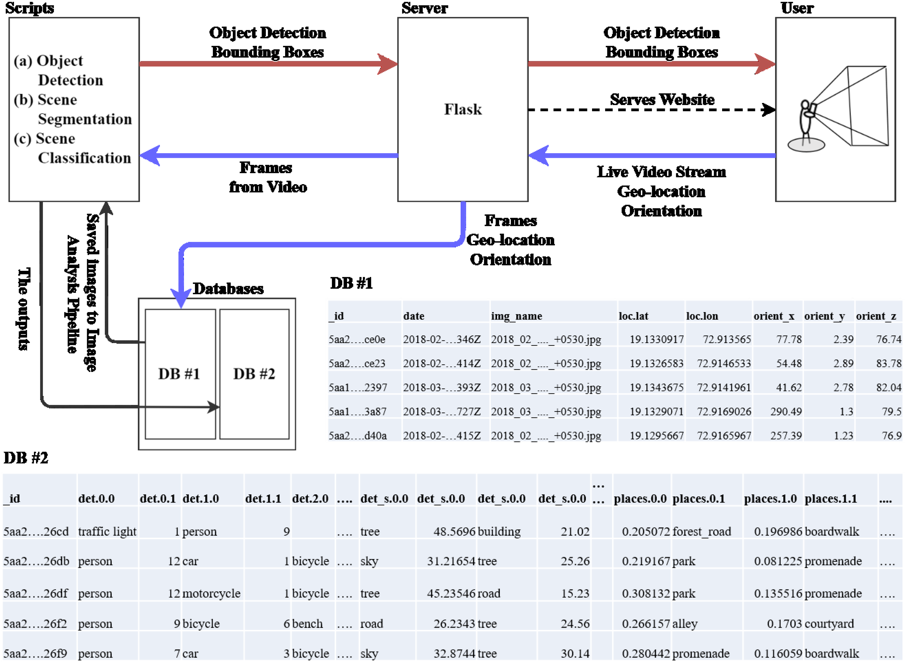
Figure 1 presents a high-level architecture of the application. We describe the workflow of the application and will cover the details in subsequent sections. The user opens up the web app through a mobile browser with an intention to collect photographs of the outdoor scenes. The application starts capturing a live video feed along with the orientation and the geolocation details from the device’s sensors. The captured data from these sensors is continuously sent to the server. The server appends the incoming data stream into the database for further analysis. The server posts back the outputs, such as detected objects, gathered from the image processing pipeline.
Apart from data collection, the intention behind the creation of the app is also to provide the user with a sense of engagement and novel value addition. This application provides real-time object detection on static and moving objects to the users while storing the video frames in the database while the app is active. At present, the application is just a proof of concept, in which application scalability and production-ready features are not administered. The application is served by a local server. To overcome device-specific security warnings regarding the use of geolocation and on-device camera in mobile devices, we used the Opera browser, which allows the application to access these sensors with minor warnings. The permanent solution to this issue would be to purchase a website domain and related security certificates. The application is tested on various entry-level Lenovo (model no. K8) and Motorola (model no. G5) smartphones. The data communication latency is checked with the help of web developer tools and Python-based timer functions. The latency statistics ranged from 0.2 s to 1.8 s, based on the quality of the internet connection available to the user’s mobile phone. The application forces the on-device camera to capture images with a resolution of 480 by 640 pixels, which can be modified to include higher resolutions. However, the quality of the images is a trade-off between the internet bandwidth and the performance of computer vision algorithms on such images. The architecture comprises: (a) A high-performance workstation acting as a server; (b) a WebRTC platform which maintains live video communication with the server. Individual frames from the video are used as the input for analysis. The WebRTC platform is actively developed and maintained, which is also cross-compatible in different mobile- and desktop-based browsers; (c) deep learning-based Python scripts which compute the outputs, which are then sent to the user (client) and the database; (d) a flask server framework to host the client webpage and the necessary scripts; (e) a MongoDB database to store and fetch the datasets. The server is chosen such that it can handle high web traffic, including the processing of incoming data, and provide outputs in real time. The server is configured with Intel Xeon, which has 32 GB of memory, along with Nvidia K2000 Graphics, with 2 GB of memory. The server runs Flask, which is a Python-based server framework. Flask is preferred over other such frameworks due to the ease in integrating the deep learning models which are based on Python. The server hosts the pretrained deep learning models and scripts which perform object detection, scene segmentation, and classification. The front-end interface of the application shows the video in the live feed from the device’s camera, while simultaneously displaying the outputs in the form of bounding boxes with labels of the objects detected in the feed.
The server handles the incoming data at two stages: (i) real-time processing of incoming data and (ii) storage of data for detailed analysis. The real-time processing utilises a lightweight object detection module (detailed in the next subsection) and produces outputs to the client. The segmentation, classification, and the main object detection module require a large amount of computational resources and time. Therefore, these modules are implemented after data is collected and stored in the database. The two-level hierarchical structure is created due to the limitations in the present hardware setup and server configuration. MongoDB is selected as a database due to its ease in the setup process. It does not require a predefined schema for data storage and can hold different types of documents in a single collection, in which the content, size, and number of fields of the document can vary from each other. Here, DB1 (
Figure 1) stores the location, device’s orientation, and captured image, which are further analysed by deep learning scripts, the results of which are stored in DB2 (
Figure 1). The list of details acquired by the application is as follows:
2.1. Device Orientation
The browser provides access to the device’s onboard sensors, such as accelerometers and magnetometers, which provide the orientation of the device with respect to Earth’s coordinate frame. The device returns alpha, beta, and gamma angles, which are the angles made by the device from the x, y, and z axes. The alpha value is the device’s heading relative to the Earth’s magnetic north. The alpha value is essential in providing the heading (direction) of a person while capturing a photograph. The values of the beta and gamma angles are required to filter out the images captured which are not focused towards the street or buildings in the proper orientation.
2.2. Geolocation
The geolocation API gives access to the installed Global Positioning System (GPS) hardware in a device. It provides locational data as a pair of latitude and longitude coordinates with accuracy in metres. The precision of the GPS is set to high accuracy to obtain continuous updates with slight changes in the user’s position. The geolocation API (
https://developer.mozilla.org/en-US/docs/Web/API/Geolocation) is based on HTML5, which works across all recent mobile browsers.
2.3. Images from the Video Stream
The video stream from the device is broken down into the individual frames for obtaining the information on the detected objects and places with the help of deep learning convolutional neural network-based models. The convolutional neural network is a variant of the artificial neural network, which is primarily used to perform image analysis. This model learns to detect the features from the provided set of image datasets to frame meaningful representations and associations. Upon training with large datasets, these models perform with near-human accuracy. Such neural network models are complex matrix operations designed to process datasets and provide predictions on specific tasks. To overcome the inconvenience of redesigning such matrix operations for every task, several prebuilt open libraries have been developed by the academia and industry. Some of the libraries are Tensorflow [
26], Pytorch [
27], Keras [
28], and Caffe [
29]. In this study, Tensorflow, Keras, and Pytorch are utilised to analyse image datasets.
2.3.1. Object Detection
We selected the object detection model based on Tensorflow due to two reasons. The Tensorflow object detection API provides detailed documentation on the usage of the detection pipeline in prebuilt image datasets as well as a custom user-based dataset. Furthermore, the large user community is active in suggesting options and alternatives to avoid the errors while working with the specific modules in the library. The typical object detection task requires weights trained on the deep learning architectures using a large database of images. In this study, these weights are downloaded from the Tensorflow official GitHub repository (
https://github.com/tensorflow/tensorflow). The repository contains a variety of pretrained weights along with the statistics on accuracy and inference-time latency metrics. The choice of latency over the accuracy depends upon the purpose and the usage. The available models have been trained on different datasets such as COCO (Common Objects in Context) [
30], Kitti [
31], and Open-Images [
32] using various state-of-the-art architectures such as ResNet [
33] and Inception [
34]. We selected COCO-based models as they included most of the objects present in the urban outdoor street view scenes, such as a person, bicycle, car, motorcycle, bus, truck, traffic light, fire hydrant, stop sign, bench, and various animals. Two models are chosen for the object detection task in this study: (a) Faster RCNN NAS [
35] and (b) Mobilenets [
36], in which the former is used for the more intensive object detection task and the latter for providing real-time inferences to the client. Faster RCNN NAS currently has the highest COCO mean average precision (an accuracy metric) amongst all the models available in the Tensorflow model zoo, thereby increasing its inference time, even with the high-performance graphic processing units (GPUs). The MobileNets model is the fastest detector amongst all the available object detector models in the Tensorflow library, but has lower precision for the detected objects. The outputs from MobileNets are not considered for scene evaluation and are utilised only for returning outputs to the mobile application. The inference script provided in the Tensorflow object detection repository (
https://github.com/tensorflow/models/tree/master/research/object_detection) is utilised as a part of the created web-based application.
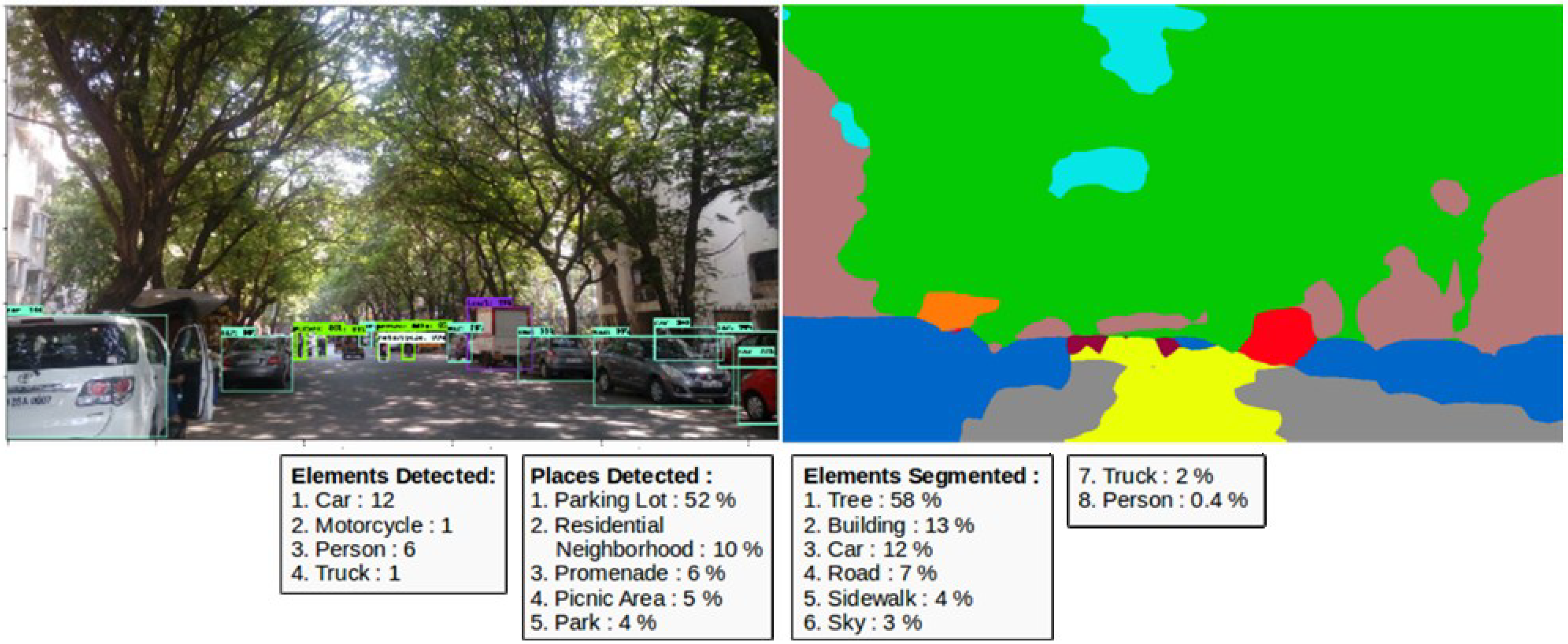
Figure 2 shows results obtained from the object detection task using the Faster RCNN NAS model. The script provides a rectangular bounding box over the elements detected and the probability of the correct detections. It is common to include a probability threshold over which the particular detected element is shown and counted by the algorithm. We randomly tried various thresholds and tested them over different street images, finally agreeing on keeping it at 20%. In other words, if the probability of detection of the element is found to be above 20% by the model, the element is detected and displayed with the bounding box.
2.3.2. Semantic Segmentation
Semantic segmentation refers to the partition of the image into meaningful predefined classes, such as sky, trees, vehicles, etc. It is a pixel-wise classification of the image (it classifies every pixel, which are then aggregated to represent the class). These created segments provide a high-level overview of the elements present in the image. Inferences such as the percentage of the scene covered by various elements can be obtained from the results of this model (
Figure 2). Among the widely used pixel-based classification techniques are Segnet [
37], FCN [
38], and Deeplab [
39]. We utilised a semantic segmentation technique based on PSPNet [
40]. The Pyramid Scene Parsing Network (PSPNet) has shown significantly better accuracy statistics on various datasets and secured the first rank on the ImageNet scene parsing challenge in 2016. The author of PSPNet has made training weights and the architecture of the model available for use in research purposes. The PSPNet architecture is trained on Pascal VOC [
41], Cityscapes [
42], and ADE20K [
43] datasets. These datasets have been widely used and researched in studies related to street view segmentation. This particular study utilised the model trained on ADE20K (
https://github.com/Vladkryvoruchko/PSPNet-Keras-tensorflow), which consists of 150 labels related to the elements present outdoors and indoors. PSPNet trained on the ADE20K dataset is chosen due to two important factors. First, the prediction time of the model trained with the ADE20K dataset is faster than other two datasets. Secondly, the classes present in the ADE20K dataset covers classes from the COCO dataset used in object detection tasks. Other common street view elements which do not feature in the COCO dataset, such as sky, trees, lampposts, and traffic signs, are present in the ADE20K dataset. The outputs from both the detection and segmentation tasks are able to capture most of the scenic attributes from street view imagery.
2.3.3. Scene Classification
The classification of a captured image into different semantic classes related to common urban places has the potential to categorise urban landscapes at a large scale. The Places dataset [
44] consists of around 10 million images depicting indoor and outdoor views. These places are classified into more than 400 classes, where each class consists of more than 5000 images. Images are trained on state-of-the-art ResNet [
33], VGG [
45], and GoogleNet [
34] architectures and the trained weights are being made available for the research community. The scene classification model used in this study is based on Places365, which is a subset of the Places database and consists of 365 classes. It classifies the images into a list of the top five classes along with the classification probability (
Figure 2). The common classes which can be detected in the scene classification are an alley, cafeteria, balcony, department stores, forest path, park, courtyard, promenade, etc. The Places database has been used by several visual perception-based studies to annotate the collected imagery into its scenic attributes. This study makes use of the working demo script provided by CSAIL (
https://github.com/CSAILVision/places365), implemented in Pytorch.
3. Prototype Implementation
To test the applicability of the designed framework in real urban scenes, we selected a geographical area of 0.25 km
2 to conduct the study. The selected area is part of an academic campus. The data collection process involved usage of the created application to collect photographs from different locations by sending streaming data to the server. Approximately 2000 photographs were collected in 12 days with the help of five volunteers, who were given access to the application to conduct the survey. The streets were predefined in the selected area for conducting the survey. However, the selection of a particular location or set of locations were at the volunteer’s discretion. There were no time restrictions on the collection of photographs, but several photographs were filtered out from the database which were sent to the server after a specific time (0600 to 1800 h) due to the lower visibility outdoors. Furthermore, the collected frames which had been tilted by around ±20 degrees in the
y-axis were filtered out with the help of database operations. Each street view scene is processed by the Python-based scripts, which provide 15–30 attributes as outputs, such as detected objects, segmented features, and places classification, with the probability of the top five classes (
Figure 1 and
Figure 2). These results are stored in the database, which creates a unique ID for every saved image and outputs along with its coordinate information. This information can be easily plotted and analysed through any Geographical Information System (GIS) based platform.
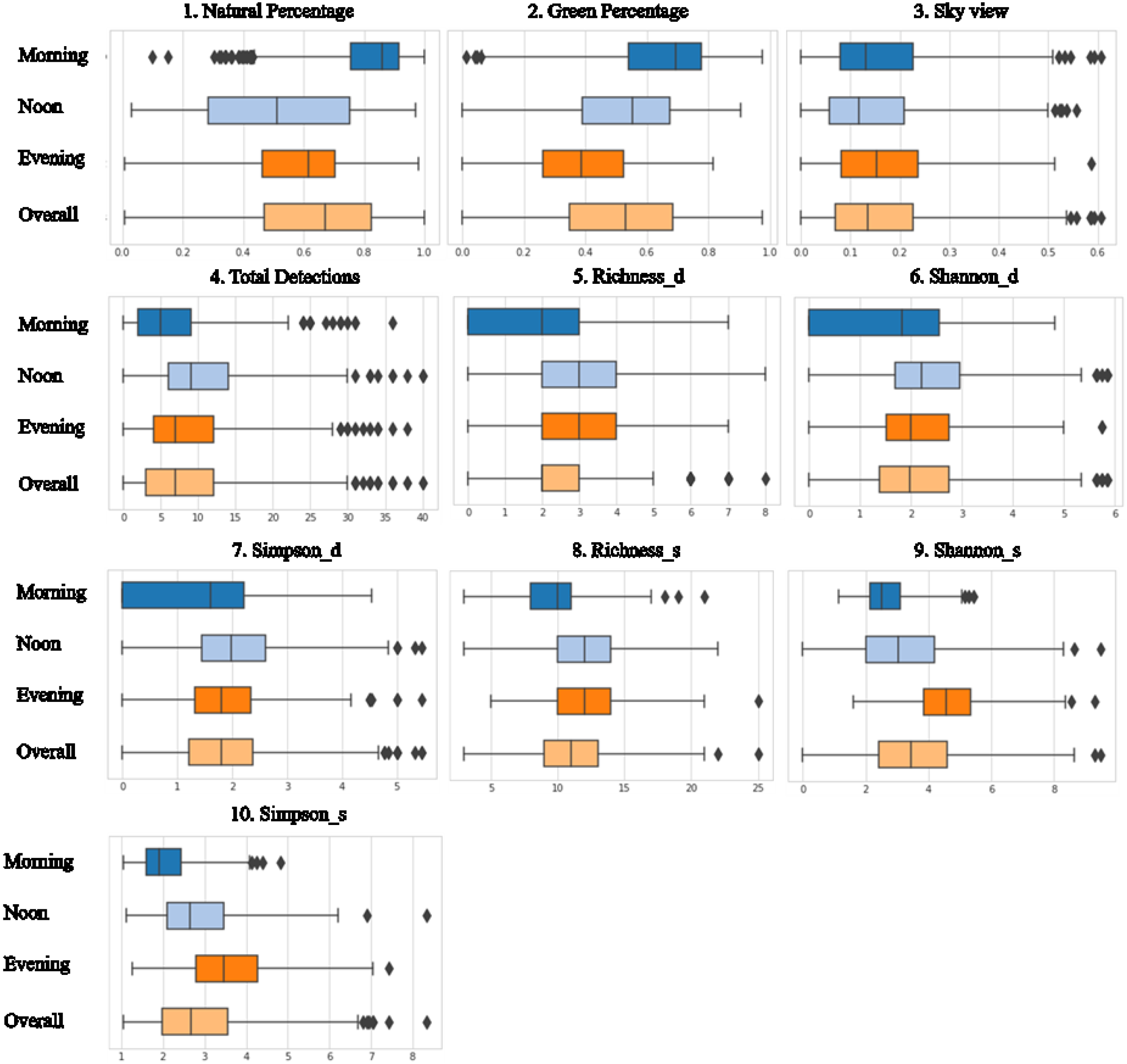
We utilised QGIS to represent our findings. QGIS provides the simple implementation of rule-based styling, labelling, and filtering, which is helpful in representing large datasets. With different attributes (results obtained from the DL pipeline) tagged to one data point, the options for its representation are endless. We calculated environment variables such as naturalness, complexity, openness, and familiarity (discussed in subsequent sections) and represented them with the help of the QGIS platform. The naturalness is calculated as the percentage of natural elements present in the scene, while complexity corresponds to the diversity of the street scenes. Similarly, openness is calculated with the sky-view factor and familiarity of the place with the image classification. Variables such as the naturalness and diversity of the scene are dependent on time, and hence show distinct outputs at different hours at the same location. Other variables such as the amount of visible sky and the places are the fixed characteristics of a particular location. The variations in data collection are recorded during different hours, as shown in
Figure A1. We segregated the collected data into three segments for comparison: morning (680 images; 0600–1100 h), noon (619 images; (1100–1500 h), and evening (794 images; 1500–1800 h). The number of images collected in each slot is nearly equal. However, we represent the comparison of time-variant variables in the morning and evening slots. To ease up the representation of the data, we aggregated the results tagged with various coordinates points with the help of a hexagon grid. Each side of the hexagon in the grid has a length of 7.5 m.
Figure 3 represents the number of collected data points aggregated under each hexagon. The number of data points ranges from 1–18. The aggregation of data points does result in an oversimplification of the inherent characteristics of the underlying data points. However, hex bins have been utilised in the representation of larger datasets for which minute details are not discernible with the naked eye.
The morning- and evening-collected datasets are not balanced for every location in the study area; therefore, hex-bin maps show slight variation at these intervals. The values calculated for various environmental variables (
Figure A1) of each data point are averaged under the superimposed hex bin. Due to the uneven distribution of data points under each hexagon, the average value might generalize the output which will result in a different colour representation of the individual bin. This method of representation might produce an erroneous depiction of dataset values. However, in this particular use case, the values do not change aggressively over their neighbouring data points. Hence, in our opinion, the hex bins are still able to represent the true character of the underlying group of data points.
3.1. Percentage of Natural Versus Human-Made Elements
The presence of naturalness in the scene is associated with the restoration of attention [
46,
47], stress recovery [
48], satisfaction, and well-being [
49]. Naturalness has been studied and shown to impart long-term psychophysical health benefits. It is also studied in preference-based studies as a scene attribute related to the perception of safety, liveliness, boredom, etc. [
50]. The presence of natural elements is one of the important elements of visual landscape assessment in neighbourhood satisfaction [
51]. In contrast to studies which related naturalness only to the presence of vegetation involving trees and grass, this study considers the composition of the scene with various other natural elements at different intervals during the day.
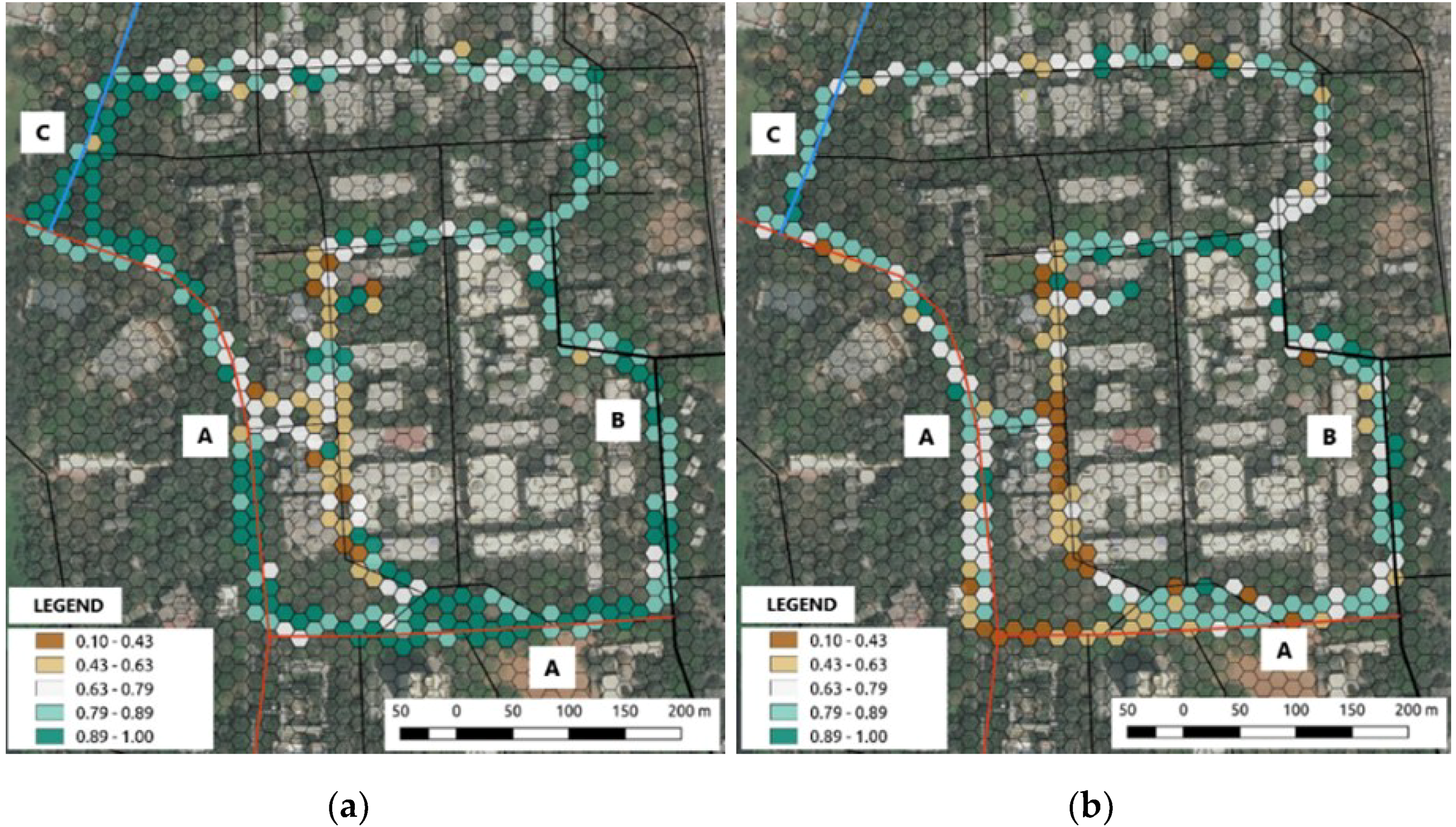
The scene segmentation task, being a pixel-wise classification, provides the percentage share of each element present in the frame, such as trees, vehicles, roads, paths, etc. These percentage values are aggregated to give the share of the natural and human-made elements in a particular scene. These values show variation with respect to the time (
Figure 4), which is expected due to the presence of different elements (such as people, vehicles, animals) in the frame taken at different time intervals. Among the 150 labels present in the ADE20K dataset, only 16 labels are based on natural elements (sky, tree, grass, earth, mountain, plant, water, sea, sand, river, flower, dirt track, land, waterfall, animal, and lake). The locations which show less variation with the time are the least dynamic locations regarding the movement of people and traffic (streets ‘B’ and ‘C’), with the opposite being true for the locations showing high variation. The street ‘A’ is a major street in the campus, which shows a significant difference in morning and evening naturalness values due to traffic peak hours at evening. The legend in the map shows the percentage of pixels covered by natural classes scaled from 0 to 1.
3.2. The Diversity of the Scene
The complexity and the visual richness of outdoor scenes have been studied in experiments related to environmental psychology and behaviour [
3]. Herzog [
52] defined the complexity of the scene as “how much of the scene contains many elements of different kinds”. It has also been considered as a prime variable of aesthetic judgements in environmental perception studies [
53]. In this study, the assessment of complexity is carried out by calculation of the diversity of urban elements present in collected street view images. Individual preferences to specific areas depend upon the presence of diversity. According to [
52], exploration of the surroundings is stimulated by the diverse surroundings. Furthermore, diversity reflects how much activity is present in a scene; “if very little is going on, preference might be lower” [
53]. In earlier studies, complexity was evaluated with the help of volunteers included as a part of on-site visual assessment surveys. The scene complexity has been calculated with the help of image attributes such as edges, features, and histograms to provide inputs on the diversity of the scene [
54]. With the help of DL techniques, individual elements can be identified with human-level accuracy, which can emulate the findings and assessments as provided by a human observer. In this study, elements in the scene are detected via two models: (a) object detection and (b) scene segmentation. The diversity metrics are calculated for each of the models according to the different types of outputs provided by these individual tasks. Object detection detects elements in the scene as separate instances of the same detected class (for example: Car: 2; Person: 3; Motorcycle: 4), whereas segmentation provides the percentage of the area covered by each class (e.g., Car: 10%; Person: 0.08%; Motorcycle: 10%).
Hill numbers are used to calculate diversity metrics due to their ease in the interpretation of diversity values. The commonly used Shannon and Simpson’s index is prone to misinterpretation of diversity due to its nonlinear nature. Hill numbers convert diversity values into effective numbers which behave linearly in relation to the changes in diversity values [
55]. The comparison of Hill numbers between any two data points (photographs) would follow the linear rule, as opposed to diversity indices other than hill numbers. The general equation of a Hill number is given as:
For diversity calculation of outputs from the segmentation task, the above expression can be interpreted as D: Diversity, p: Proportion of class to total detected classes, and s: the total number of classes detected.
q = 0 represents the richness of elements. It provides information on unique elements detected in the scene. For example, a scene having (Car: 20%; Person: 5%; Motorcycle: 35%) has the richness of 3.
q = 1 represents the exponential of the Shannon entropy index. It weighs each class according to the frequency or weights of the present elements [
55,
56]. High entropy values indicate randomness, while lower values show order.
q = 2 represents the inverse of the Simpson concentration index. It is more sensitive to dominant classes detected in the scene. The formula includes the sum of squares for which the lower values of detected elements become insignificant.
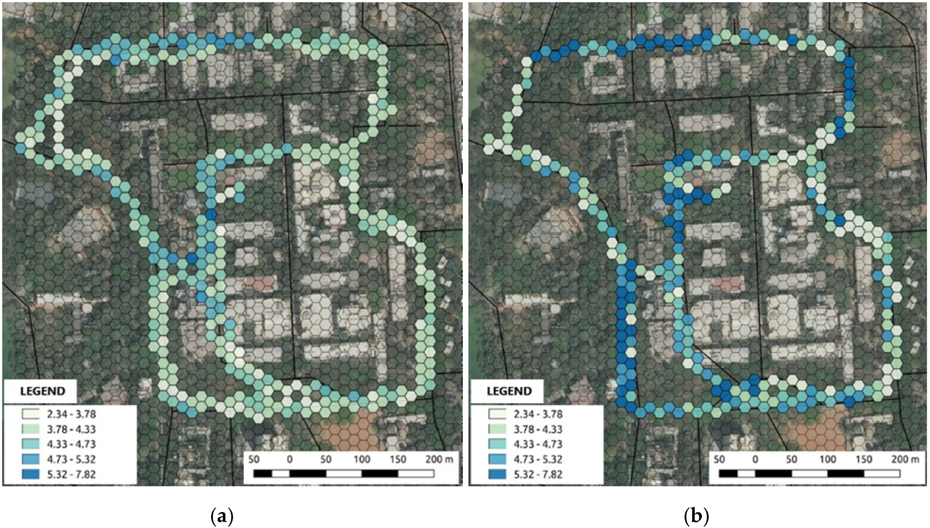
Figure 5 shows the difference between entropy (exponential of the Shannon entropy index) values calculated on elements obtained from the segmentation task. The entropy values range from 2.3 to 7.8. The difference between the entropy values at morning and evening hours suggests that (a) a lower number of elements is detected in the morning hours compared to in the evening hours; (b) the amount (percentage area in a scene) of natural elements present in the scene is higher in the morning than in the evening. The natural elements such as trees and sky amount for the maximum coverage in a scene, and due to the absence of elements such as people, buses, and motorcycles during the morning hours, the variability of the scene is lower.
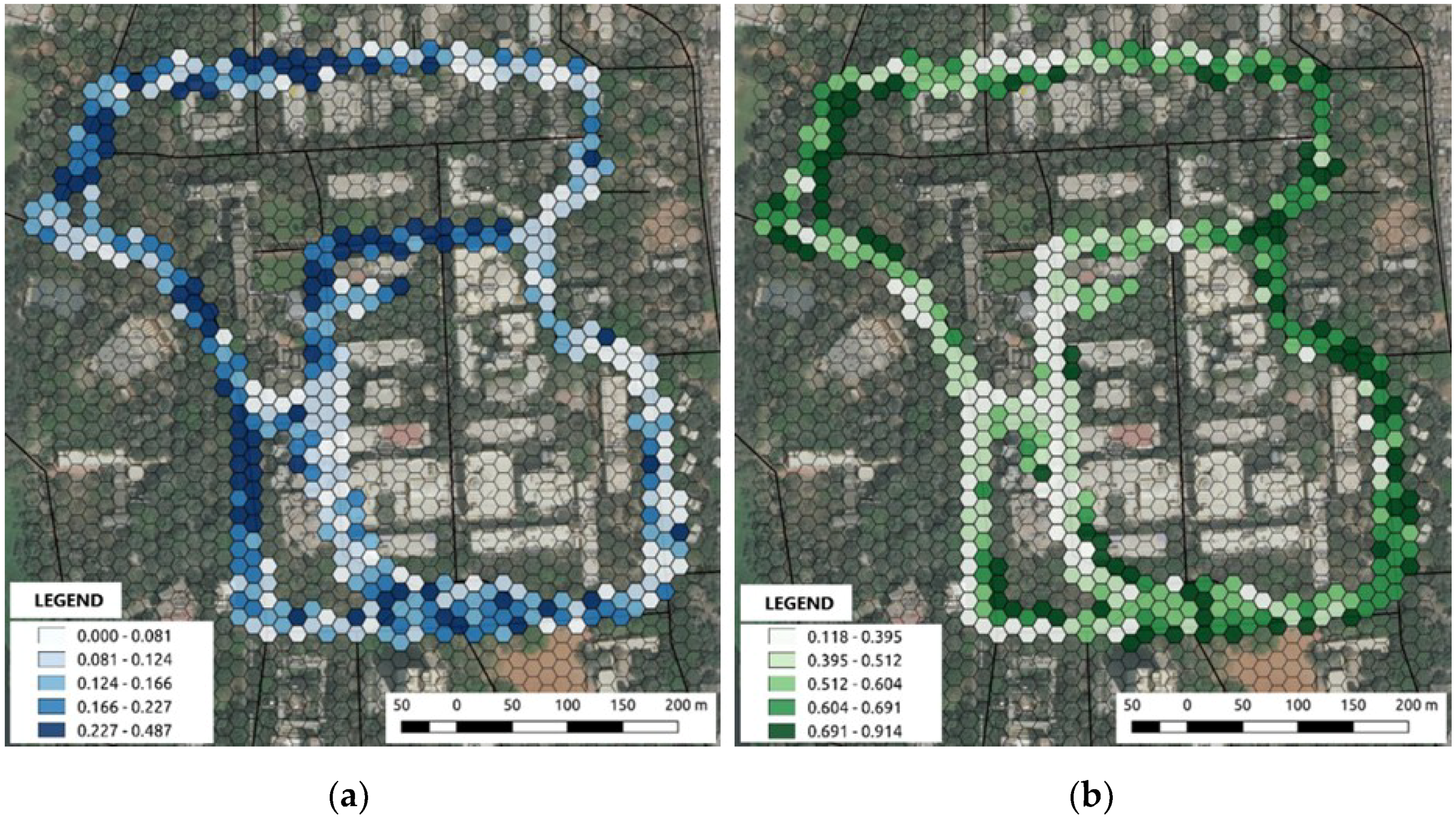
3.3. Visible Sky and Green
The amount of visible sky and the green content elucidates the scene properties such as openness, depth, enclosure and expansiveness, etc. [
57]. The sky view factor has been one of the essential parameters in studies related to the design and planning of urban structures [
58]. The effect of visible sky and green cover has been studied explicitly in preference-based studies as it had been a prime constituent of assessment of the variables such as prospect and refuge [
59]. The feelings of safety and pleasure are derived from surroundings providing a sense of enclosure and views [
60]. Studies such as [
13] have created tools to analyse the sky–green ratios for cities, which help urban planners to explore urban areas with interactive visual analysis. Visible sky and green percentages are extracted from the scene segmentation task. The range of values (0–0.48) in the percentage of sky view is lesser than that of the presence of a green character (0.1–0.91) of streets. The value of green cover calculated from scene segmentation should not vary with time; however, the variation in the morning, noon, and evening green percentage values are recorded (
Figure A1), due to the presence of other street elements in the collected photographs at different timings. In contrast, the sky view factor only has a slight variation (
Figure A1), as expected, in the values at different times. The higher percentage (
Figure 6) of the visible sky and green cover at some locations can be interpreted in two ways: being due to (a) the absence of high-rise built structures and trees; and (b) the absence of human-made elements along the streets and huge green canopy cover over the street, respectively. Also, the low green cover with high sky view percentage may suggest the presence of openness, while the low green cover and low sky view percentage may provide a sense of enclosure. The assessment of greenness through street view imagery is helpful in identifying the green coverage which is within visual reach of the people.
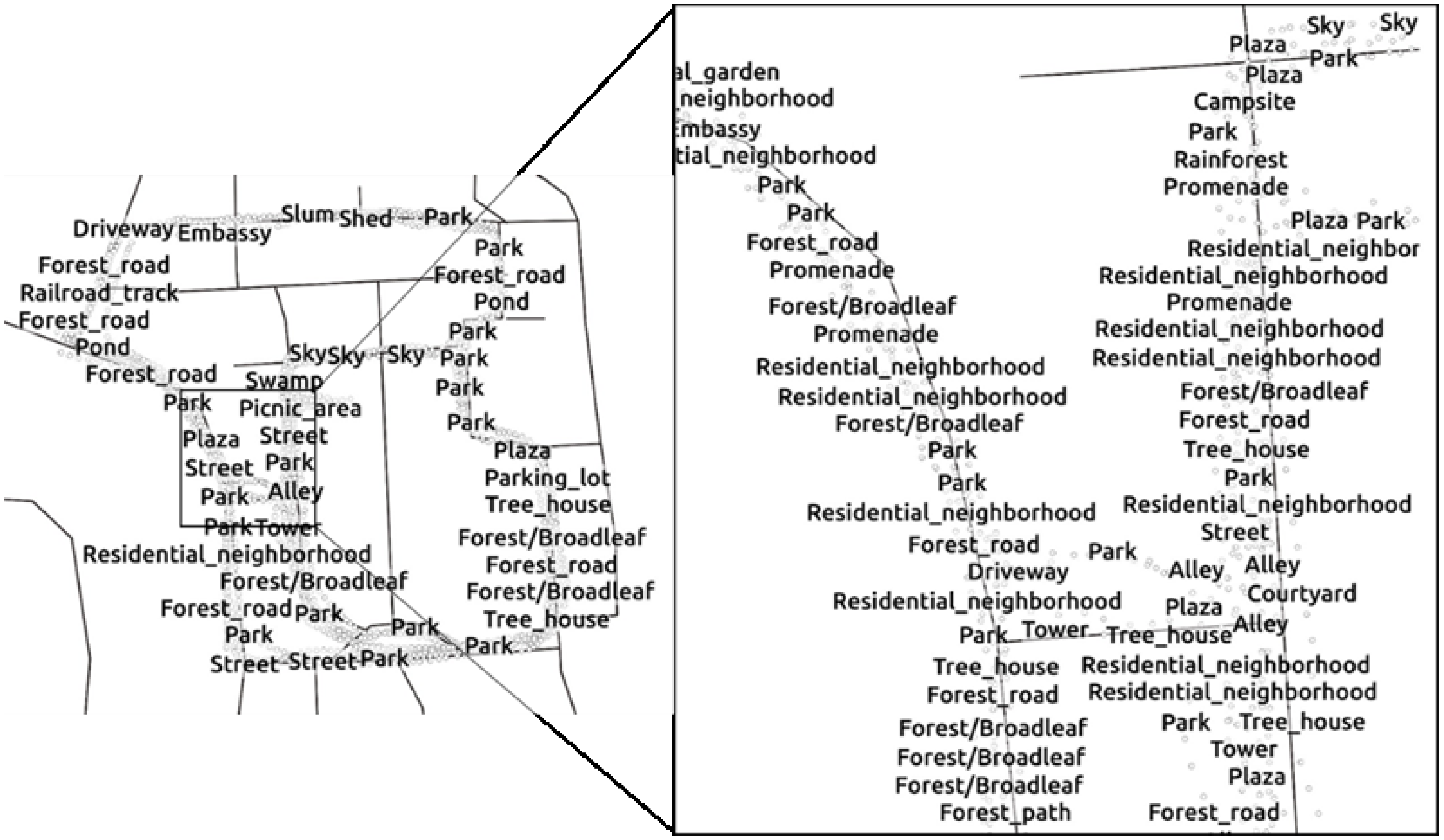
3.4. The Places Present in the Scene
Preference to the particular scene is affected due to the presence of familiar and unfamiliar urban places in it [
9,
61]. The variables such as familiarity, identifiability, and novelty have been studied in urban scenes containing restaurants, coffee shops, factories, apartments, etc. The presence of particular places also acts as an element of mental, cognitive maps which people continuously utilise to travel around [
62]. The presence of such places may induce the feeling of safety, liveliness, or boredom (for example, the presence of factories and alleys induce a feeling of desolation [
61]). Classification of such places is done with the help of the scene classification task. The study area has a significant amount of green cover and identical built structures compared to any general urban area; therefore, the classes such as forest road, embassy, and courtyard are present in dominance.
Figure 7 represents the most dominant classes present in the particular location.
4. Data Analysis and Limitations
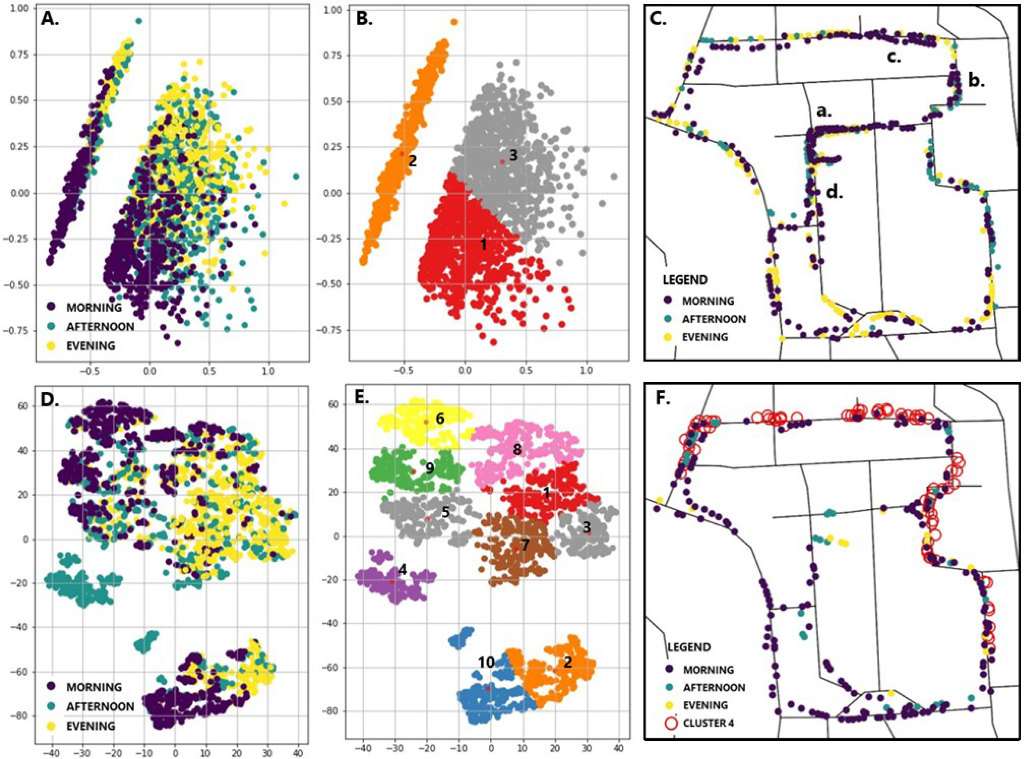
The differences and similarities in scenic attributes between different data points are explored through clustering algorithms such as principal component analysis (PCA) and t-distributed stochastic neighbour embedding (t-SNE). PCA is a dimensionality reduction technique which removes the redundant dimensions to keep a new set of calculated linear independent dimensions known as principal components. The values of these dimensions can be plotted in 2-D and 3-D for visualisation. Ten parameters of each data point are considered, which included three values of hill numbers, each calculated from segmentation and detection tasks; the number of total elements detected from the detection task; and the percentage of green, naturalness, and the sky view. Most of these parameters are intrinsically correlated with each other, such as the percentage of green being a subset of naturalness. Similarly, Simpson and Shannon indices of hill numbers also show high correlation. PCA was implemented in the Scikit-Learn Library (
http://scikit-learn.org/) to identify key influencing parameters using 2093 data points. The parameters were normalised before processing. The scatter plot (
Figure 8A) shows the plot between the first and second principal component. Three different colours indicate the timings (morning, noon, and evening) of the captured data points. The plot shows two distinct clusters significantly different in size. In order to identify characteristics of the clusters, the K-means algorithm was implemented to delineate the clusters. K-Means is an unsupervised algorithm which is used to find groups in the datasets. The smaller cluster (cluster no. 2 in
Figure 8B) consists of data points for which the object detection task resulted in zero detections, due to dependent parameters such as Hill numbers producing a value of zero. The cluster consists of images collected from all the three timings. The data points in the cluster are plotted against the map for visual assessment of the association between points at different locations. Most numbers of zero-detections occurred in the morning (225), followed by the evening (162). The peculiar case of the least number (94) of zero-detections in the afternoon can be attributed to the increased street activity due to vehicles, people, and bicycles during class hours in the campus. Furthermore, the locations of zero-detections (a, b, c, and d) lie in the inner streets, which are usually deserted during the morning hours.
Additionally, t-SNE clustering is implemented with the help of Scikit-Learn to gather more specific patterns and clusters in the dataset. t-SNE is a nonlinear dimensionality reduction technique which computes differences between points and tries to maintain them in low-dimensional space [
63]. However, t-SNE does not preserve distances or density information, which makes it challenging to analyse and interpret the appropriateness of the clusters calculated by this algorithm. The clusters (
Figure 8D) are not perfectly resolved and discernible. To inquire about a particular group of data points having similar attributes, we performed K-means to create clusters of the t-SNE results. We are aware of the fact that K-means, being a distance-based clustering algorithm, may produce errors while delineating borders of the t-SNE clusters due to loss of distance-specific information while implementing the t-SNE algorithm. Cluster nos. 1, 2, 3, and 7 do consist of a large share of points collected in the evening, while 6, 9, and 10 are the same for morning data. The clusters 10 and 2 contain the points which have the properties of PCA cluster 2. Some of the data points collected in the afternoon produce a visually distinct cluster (no. 4). On plotting the same on the adjoining map, it shows the location of these points. The distinctness of the cluster is due to the similarity between the values of environmental variables. The particular locations of the street have similar characteristics regarding the on-street parking, high canopy cover, and low sky view percentages. Similarly, cluster no. 6 was randomly chosen and plotted in the map. Unlike the cluster no. 4, which shows distinctness in the values at specific locations, the precise characteristics of the cluster are difficult to ascertain; however, all the included points fall in the range consisting of low diversity (Shannon_s in
Figure A1) below 3.5 and richness (Richness_s in
Figure A1) below 15, but do vary in variables such as the percentage of sky view and total detection of elements (
Figure A1). The adjoining map shows that the locations of the points are scattered all over the area, which does not suggest that any particular street has similar data points.
The results in the study are based on the unequal observations taken at different locations, due to which, some of the inferences regarding the diversity and variation differ. However, PCA and t-SNE-generated clusters show that the dataset is not randomly dispersed, where attributes of points similar to each other provide meaningful associations. The data collection is conducted by a small number of participants in a smaller and managed institutional environment. A typical urban area, on the other hand, is more dynamic and diverse regarding the traffic movement and includes a different set of factors which may be interrelated as well as random. Reflecting such details in the experiment is achievable with the large user base and computational power. The lighting conditions, even during daylight, are scarce in certain pockets overshadowed by green canopy cover or tall buildings, due to which, particular objects may not be detected even if they are present. Occlusion is a widely researched phenomenon in computer vision, in which the detection of the object depends upon the visibility of the objects to the camera sensor. The detection of objects is compromised if they are partially hidden behind other objects. The models used in the study are not tested in the field for the occlusion and related technical insufficiencies. Due to this, the outputs may vary regarding the choice of the street for surveying purposes. The web-based mobile application is based on open-source modules and frameworks which are widely researched and utilised both in academia and industries. Such an application can be expanded significantly with the use of technologies and expertise not available to the authors. The individual modules of deep learning methods are a constant subject of research and do possess high chances of the development of newer and efficient models. The deep learning models used in the study may be replaced by different methods and practices over time.
5. Discussion
Urban perception studies aim to understand the relationship between the presence of scenic elements and the perceptual attributes of the environment, such as safety, liveliness, boredom, wealthiness, depressing, and beautiful. Earlier studies have established several constructs, such as the presence of naturalness stimulating satisfaction, or the liveliness present in the street increasing safety; however, none of these have been validated by large-scale perception-based research. The collection of data and the identification of low-level physical features has always been a key determinant in such studies. This study provided an example to conduct rapid data collection and visual data analysis with the state-of-the-art methods and tools. Special focus was given to create a dataset which is spatially and temporally rigorous. Mapping the transient nature of urban spaces is essential in studying the urban environment in a detailed manner.
The analysis of low-level features present in the street view scenes has an immense potential to aid researchers and city managers to focus on bottom-up urban planning approaches. The tasks of asset management and spatial planning regulations are largely based on land use land cover (LULC) maps, which provide information regarding the form and function of the city. This study proposed a methodology to generate maps of low-level physical features as visible from the individual’s perspective. The visual access to different environmental attributes such as the greenness, built character, and type of urban places may help in the quantification of physical features which cannot be mapped in LULC maps. Automated map generation and its revision can be achieved with the help of such an application. Apart from data collection, the application can be extended to include real-time user-provided ratings to the places based on the different perceptual attributes. Identification of environmental variables coupled with the user’s perception of the space may provide a hint on the socioeconomic conditions of the neighbourhood. It may help to identify the disparity in perceptions which may be due to criminal activities, health, high population density, and ethnic composition.
The quality of life has been studied as the relationship of a person with the environment, where the access to greenery and open spaces plays an important role in determining satisfaction and happiness. Furthermore, the analysis of visual aesthetics such as the identification of dominant colors, landscaping, built façades, and dilapidation of built structures is helpful in studying and creating aesthetically pleasing experiences. In the longer term, such a framework deployed with a large user base may ensure the rapid mapping and auditing of such changes in the environment. It will help in providing data-driven suggestions to the urban management about the places in need of redevelopment and retrofitting.
6. Conclusions and Future Work
We presented a framework aimed towards data collection and representation of the findings. This study is an attempt to quantify environmental attributes through technological means. We provided examples to assess high-level variables such as naturalness, complexity, familiarity, and openness with computer vision techniques. We focused on discussing various environmental variables and visual properties which influences people’s preferences and play an important role in an individual’s quality of life. Rigorous statistical and spatial analysis of the obtained results is the way forward for future research. This study, although limited to smaller premises, holds the potential to be scaled up at the city level. The web application presented in this study can be redesigned with personalisation and user experience features which can be scaled to involve more users for large-scale studies. City managers can utilize this framework to collect street-level datasets to gather detailed characteristics of the city with the help of a large number of users. The proposed framework can be integrated with the already existing mobile-based city guide applications. Recently, the deep learning frameworks have been deployed in the Android- and iOS-based mobile platforms, which do not require dedicated server support for data processing. Future studies may utilize this native platform support to showcase different features. This study is purely based on identifying visual cues in the surroundings. However, the environment perception is a collective response to different human senses. Along with the visual, auditory and olfactory realms play a significant role in preference towards specific spaces. Future studies may include the collection of these multimodal datasets for the comprehensive evaluation of surroundings. Lack of tools and techniques to understand the rapidly changing urban landscapes has been a major impediment to its planning and management. Results from such studies may discover the unavailability or inadequacy of specific environment variables essential for human health and well-being.


