Article

Towards a Unified Currency for Landscape Performance Evaluation: A New Zealand Case

1
School of Landscape Architecture, Faculty of Environment, Society and Design, Lincoln University, Lincoln 7647, New Zealand
2
Faculty of Agribusiness and Commerce, Lincoln University, Lincoln 7647, New Zealand
3
TRADE Research Focus Area, North-West University, Potchefstroom 2531, South Africa
*
Authors to whom correspondence should be addressed.
Urban Sci. 2026, 10(1), 7; https://doi.org/10.3390/urbansci10010007
Submission received: 17 October 2025 / Revised: 28 November 2025 / Accepted: 8 December 2025 / Published: 24 December 2025

Abstract

Landscape Performance Evaluation (LPE) practices have made significant progress over the past decade. However, challenges persist in comparing landscape benefits and conducting cost–benefit analyses for decision-making. This paper introduces a “universal currency” for comparing landscape benefits and weighing them against costs. Employing a revealed-preference approach, this study quantifies the perceived benefits of public open spaces in a fast-growing peri-urban town in New Zealand by analysing their impact on land values. The findings reveal a positive correlation between proximity to public open spaces and increased land prices, highlighting the potential of economic indicators for unifying landscape benefit measurements. An analysis of 15-year historical geoinformation and transaction data further demonstrates the consistency of the contributions, even during major market disruptions, showing the robustness of the monetary indicator. This exploration, while offering a pathway toward more effective landscape performance evaluation practices, also underscores the critical role of landscape architecture in enhancing human well-being.

1. Introduction

Over the past half-century, modern landscape architecture, as a young discipline, has rapidly evolved, with pioneer researchers and practitioners pushing its boundaries in diverse directions [1,2,3,4,5,6]. The wide range of benefits that landscape architecture interventions can offer is increasingly recognised and acknowledged by scholars, practitioners, authorities, and the general public [7,8]. The recognition and acknowledgement extend to environmental, economic, and socio-cultural values [8,9].
With the growing number of claims for benefits that can be offered by landscape architecture interventions, there was also a corresponding rise in the demand for evidence to substantiate these claims [7,10,11,12]. Since 2010, there have been collaborative endeavours in landscape performance evaluations that have contributed significantly to the measurement of landscape benefits, thereby providing evidence for future landscape architecture practice. Of particular importance is the Landscape Architecture Foundation (LAF)’s Case Study Investigation (CSI) programme, a collaborative endeavour which is building incremental knowledge on landscape performance [13,14,15]. Over the past decade, the CSI programme has funded more than 190 Landscape Performance Evaluation (LPE) projects, built up perhaps the most extensive landscape performance database, and iteratively developed an evaluation framework that has guided hundreds of LPE projects and continues to influence ongoing performance evaluation endeavours in the field as flagship guidelines [9,13]. Landscape Performance Evaluation (LPE) refers to the systematic assessment of the benefits generated by designed environments, which can include environmental, social, cultural, and economic benefits [8,13,16]. LPEs are often conducted to examine how effectively landscape interventions achieve intended outcomes and contribute to human wellbeing [8,16].
Apart from the CSI initiative, similar efforts have also emerged internationally in different forms. For example, performance-focused approaches have been integrated into landscape planning and assessment frameworks in Europe [17,18], China [13], and Australia [19] through ecosystem services and planning assessment initiatives, etc. In New Zealand, while there is no dedicated LPE framework or programme, such practices are also conducted sporadically [16,20,21]. These international developments also demonstrate a global shift toward evidence-based landscape evaluation and practice. However, the current LPE practices still face some methodological challenges that limit their effectiveness for evidence-based decision-making and planning.
Drawing upon a 2021 CSI evaluation conducted by Bowring and Chen [22], Chen, Bowring and Davis [12] shared their reflections on adopting the LAF’s flagship evaluation framework for their CSI evaluation, as well as their observations related to the methods and results of some past CSI evaluations they studied during their CSI research process. Their study identified two key challenges hindering LPE practices from achieving their full potential and meeting their purposes of providing evidence for future landscape developments and better communicating landscape developments’ contributions to human wellbeing.
The first challenge lies in the difficulty of comparing the landscape benefits with their associated costs [12]. Over the past decade, LPE practices have made substantial progress in quantifying landscape benefits—the benefits of many landscape architecture projects were quantified, clearly communicated, and celebrated as evidence for high-performing landscape architecture practices [9,12]. However, the assumption often defaults to viewing any improvements as positive, without comparing them to the associated costs [23]. The key reason related to this is the mismatch in measurement units—under the current evaluation framework, benefits are often measured using various measurement units, such as tons of sequestrated carbon, pounds of reduced downstream nitrogen, and percentages of users with improved quality of life, while their associated costs are typically measured in monetary terms [12,23]. As a result, the quantified benefits are not comparable with their costs, and even when benefits are quantified, there is no clear threshold for determining how large they must be for a project or a design intervention to be considered cost-effective and deemed “successful” [23]. The absence of a clear threshold for justifying costs against benefits undermines the effectiveness of using quantified landscape benefits as evidence to demonstrate design excellence or provide evidence for decision-making [23].
Apart from the difficulty in justifying costs against benefits, the aforementioned nonuniform measurement units of landscape benefits also hinder comparisons between different benefits, presenting a second challenge [12]. The absence of a “universal currency” or a “common metric” capable of bridging the unit difference among diverse benefit measurements makes it almost impossible to compare one benefit with another [12,24]. In this study, universal currency refers to the standardisation of different benefit measurements that enables the comparison of otherwise incomparable benefits. The absence of such measurements becomes particularly pertinent when facing limited investment and when priorities must be set, which is a constant reality in practice, where resource scarcity always necessitates decisions on priorities [12,25,26]. In the absence of a comparative framework, the opportunity costs associated with each of these benefits remain unaccounted for under the current evaluation frameworks. Research in environmental economics indicates that without a “universal currency”, benefit evaluations may lead to suboptimal decisions, as alternatives are not assessed on a comparable basis [26]. In other words, while all quantified benefits present a positive outlook, it is still insufficient to support claims that a landscape intervention is “successful” in terms of resource allocation [12,26]. Without a “universal currency” that would allow for one benefit to be comparable with another, the evaluations conducted under the existing framework offer little insight into whether more significant benefits could have been achieved by allocating the same resources in other ways [12]. Translating different landscape benefits into a common measurement can help planners and decision makers to better understand the trade-offs between different development options [25]. Despite these recognised challenges, there remains a notable gap in empirical studies to test practical approaches for translating different landscape benefits into a comparable evaluative measurement.
As a means of exploring these two challenges, this paper focuses on a particular case study to identify how benefits measured in diverse ways could be translated into monetary terms—a form of “universal currency”—to enhance comparability. Such monetary expressions serve as an effective vehicle to make different landscape benefits comparable [24]. This research assesses the monetary value of the perceived benefits of public open spaces in Lincoln Township, Canterbury, New Zealand. In this study, “public open space” is defined as publicly accessible, non-commercial outdoor green space intended for recreational passive use. It includes neighbourhood parks and reserves but excludes playgrounds and sports fields. These excluded spaces, which serve active recreational functions and attract activity-specific users, generate value contribution patterns that differ from the broader landscape amenity this study aims to capture. Restricting public open space to passive, non-specialised open spaces ensures that the hedonic model focuses on general landscape-related amenity rather than facility-driven preferences. By separating them, our model was able to assess their influence individually. The public open spaces in Lincoln referred to in this paper are all planned or artificially managed for delivering multiple landscape benefits, including socio-cultural benefits. Lincoln was selected as the study area for two reasons. Firstly, Lincoln offers a relatively controlled environment for our statistical analysis—it is topographically flat, and the housing developments there are mostly single-story dwellings. This homogeneity reduces the number of variables (such as varying building types, vertical structures, and visual accessibility differences resulting from topography and vertical structure differences) and the complexity of the statistical modelling. Secondly, Lincoln is also a representative case in the growth context of many New Zealand peri-urban towns, as well as a similar context overseas, where planners and decision makers face decisions about investing in landscape amenities. Insights from Lincoln can be informative beyond this case. Lincoln’s popularity created a competitive residential market, leading to an increased use of landscape architecture design for public open spaces in new residential subdivisions to establish market differentiation. The use of monetary value as a “universal currency” contributes to the ongoing endeavour to address the two identified challenges related to benefit measurements.
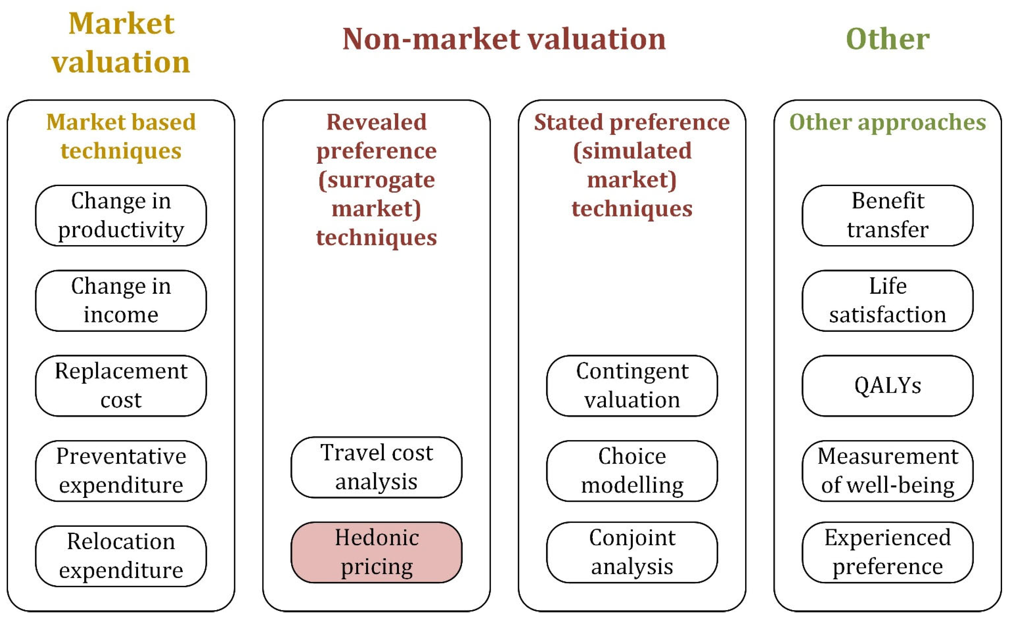
Other disciplines overcame the challenges of measuring heterogeneous goods by identifying and isolating variables that can be measured. This created two broad approaches to identify value, namely market valuation and non-market valuation. This study applies a non-market valuation approach (see Figure 1) through a hedonic price model to assess how market participants value landscape design through property market transactions. It is noteworthy that this study does not define landscape performance solely in economic terms. Instead, the economic valuation we applied here serves as a methodological exploration, which examines whether monetary indicators can function as one possible universal metric representing the broader environmental, social, cultural, and economic dimensions recognised within LPE.
The objective of this study is to empirically examine whether this monetary valuation can function as a “universal currency” that enables comparison across different landscape benefits and between benefits and their associated costs. This inquiry contributes to LPE literature by testing an environmental economics approach that could improve benefit justification, enhance comparability between projects, and strengthen cost–benefit reasoning in landscape design and planning. By employing the hedonic pricing model approach, this study analyses how the perceived benefits provided by the public open spaces within the local township of our study site are reflected in the transactional data of the real estate sales that occurred over a 15-year period. Further, instead of using the capital value of the properties, we use the land value for our hedonic model analysis. In doing so, this study is unique in focusing on land values rather than capital values. This allows us to isolate the contribution of the structural differences (i.e., the buildings themselves), making the dependent variable more relevant. Also, the study’s originality is further reinforced by our longitudinal study design, which is rare in the literature. The 15-year longitudinal analyses allow us to observe how amenity value premiums persist or fluctuate under changing market conditions over time. Through this analysis, this paper indicates the monetary value of the perceived benefits of public open spaces (which include improved mood and quality of life, opportunities for physical activities, and aesthetic and amenity values, etc., as identified by Bowring and Chen [22]) and also explores how the value changes over time.
This study is situated at the intersection of environmental economics, planning, and landscape architecture—disciplines that share a common interest in better understanding how landscape amenities enhance human wellbeing yet often approach this question through different methodological traditions. Despite increasing calls for evidence-based landscape evaluation [16,21,27], empirical techniques capable of converting diverse landscape benefits into a unified evaluative metric remain limited. By integrating the hedonic pricing approach with landscape performance evaluation, this study seeks to establish an analytical pathway for translating various landscape benefits into a standardised and comparable form, thereby helping to bridge existing methodological gaps and strengthen the foundations of evidence-based evaluation.

2. Literature

While assessing the monetary value of landscape benefits is a recent development in the field of landscape architecture, similar ideas have been broadly examined in the fields of land use planning, property, ecology, and conservation. A range of items have been explored for monetising their associated benefits, including trees [28], forests [29,30,31,32], green spaces [28,33,34], waterbodies [28,35,36,37,38,39,40], scenic views [41,42], recreation areas [43], linear infrastructure [44], and school districts [45]. Apart from the physical items, some specific categories of benefits have also been monetised, such as air quality improvements [30,31,46,47,48,49], water flow regulation [32], urban cooling [31,46,50], noise reduction [51], and carbon sequestration [22,23,31,48,52].
Despite the evolution of the monetisation/capitalisation literature, it has yet to cover all realms of value [53]. In comparison to tangible benefits like the ones mentioned earlier, intangible benefits are often more challenging to quantify and thereby receive less attention in practice [53]. Although intangible benefits (including a variety of socio-cultural benefits) are incorporated in almost all value frameworks (e.g., ecosystem services, sustainability, and LAF’s CSI evaluation framework) [54,55,56,57,58], without the support of capitalised empirical evidence, these intangible benefits are less competitive in the decision-making process compared to the tangible ones and are thereby often undervalued or excluded from valuation [53]. However, an especially significant portion of the benefits derived from landscape architecture projects are intangible, adding a layer of complexity to the valuation of landscape benefits. As Corkery [19] noted, assessing such intangible benefits requires “a sensitive approach to gathering evidence of tangible benefits”. This difficulty is also highlighted by Deming [59], who noted “wherever intangibility is a factor in research, it can pose special intellectual and practical research challenges that demand creativity and subtlety in response”. Despite this difficulty, conquering the challenge is crucial to ensure that intangible benefits, a substantial part of landscape values, are not overlooked in the decision-making process. This allows for the application of existing value measuring techniques used in the extant literature from various other disciplines in landscape performance evaluation. As documented by the LAF’s guidebook for LPE metrics and methods [56], landscape interventions can offer a range of intangible benefits such as aesthetic values, recreational opportunities, health and wellbeing benefits, noise mitigation, cultural preservation, and educational opportunities. The intangibility of such landscape benefits often makes them difficult to measure directly. However, economic theory provides a basis for inferring the value of such benefits through observable market behaviours. According to hedonic price theory, buyers or residents evaluate properties as a bundle of attributes and are willing to pay price premiums for characteristics that contribute to human wellbeing, such as recreational opportunities and amenity value [60,61]. A wide range of empirical studies [33,34,37,38,39,40,41,42,43] show that the housing market captures the value contribution of a wide range of environmental and landscape attributes. These studies [33,34,37,38,39,40,41,42,43] demonstrate that when landscape features improve residents’ perceived wellbeing or provide desirable amenities, these contributions are reflected in market transactions, allowing intangible non-market landscape benefits to be inferred from sales prices. In this sense, a hedonic price model can serve as a defensible approach for capturing the perceived value of intangible landscape benefits.
In parallel with the monetisation approach, recent spatial planning approaches also highlight the value of integrating ecosystem service assessments into land-use decisions. For instance, Córdoba Hernández and Camerin [62] propose a flexible planning framework that uses ecosystem service information to justify ecosystem protection efforts. However, on the other side of this debate, some scholars urge caution against the exclusive monetisation of environmental and cultural values. There is an ongoing dialogue in the literature about the limitations of purely economic valuation, including noted tensions between economic efficiency and social equity considerations. For example, Chan, Satterfield, and Goldstein [53] advocate incorporating dimensions such as moral notions into ecosystem service valuation frameworks, arguing that a purely economic metric is inherently incomplete in scope. Douglas McCauley [63] cautions that an over-reliance on monetary metrics may overlook or undervalue qualities that are difficult to quantify. By acknowledging various viewpoints in the literature, we clarify that our proposed metric is presented with an understanding of its limitations and the need for complementary qualitative judgments. We would also like to highlight that employing monetary valuation methods is a deliberate methodological choice: such approaches are widely recognised in research and practice globally, providing a common currency that reflects societal preferences and environmental preferences [24,64,65,66,67,68]. Monetary values enable direct comparisons between costs and benefits, as well as between different benefits. Therefore, despite their acknowledged limitations, monetary indicators remain a practical and robust tool for integrating non-market or intangible benefits into decision-making processes.

3. Material and Methods

As aforementioned, intangible benefits are often challenging to measure because they are normally in non-commercial form and are not tradable in the market. However, there are some possible approaches that can help measure these intangible benefits indirectly. Figure 1 adapted from Clough and Bealing [69] outlines common valuation approaches used in practice. Among these, non-market valuation approaches are particularly relevant, as they enable the translation of intangible benefits into monetary values, making them comparable with other tangible ones, as well as the costs, which are often measured in monetary terms. This study adopts the revealed-preference method, which entails assessing the value that the users of an environment assign to it by examining their in-market purchasing behaviours that relate to the characteristics of the environment [70,71]. The chosen value indicator (i.e., the in-market purchasing behaviours) for this study is the transactions of land properties, whose market values are closely tied to various environmental characteristics, such as the proximity to public open spaces, green space and waterbodies. The land value of properties is adopted in this study as it focuses on the locational, rather than structural characteristics. This type of approach is commonly referred to as the hedonic pricing model and is often employed to estimate the value of features pertaining to the surrounding environment of the property [72,73]. The hedonic pricing approach is a widely accepted approach, and particularly in comparison to other approaches, it offers the advantage of basing the valuation on observed actual behaviours of individuals who perceive and respond to the intangible landscape benefits [74]. The hedonic model is especially well-suited to the conditions of the landscape amenities examined in this study.
Figure 1. Common valuation methods used in practice. Adapted from Clough and Bealing [69]. The hedonic pricing model, as highlighted, was the valuation approach employed in this study.
Urbansci 10 00007 g001
This study developed a series of regression models using transactional data from real estate sales and geolocation data. These regression models were developed to analyse and explain how public open spaces, as an independent variable, along with other locational variables, affect the dependent variable, the price of the adjacent residential lands. Additionally, this research also investigated the temporal changes in this perceived value over the 15-year study period. This section outlines the process of how the data were acquired, generated, processed, and eventually statistically analysed.

3.1. Study Site

The study site, Lincoln, is a town located in the Canterbury region of New Zealand’s South Island. Lincoln has a population of 10,250 at a density of about 1100 people per square kilometre [75]. The residential developments in Lincoln are particularly conducive to the employment of the hedonic pricing model due to their topographical and building homogeneity. Firstly, the town is located on the Canterbury Plains, characterised by a very flat landform (as shown in Figure 2). Consequently, properties within Lincoln town exhibit very similar elevations and topography, which reduces the number of variables that have to be introduced to the statistical model. Secondly, almost all the residential buildings in Lincoln are low-density single-storey buildings (as shown in Figure 2), which eliminates the impacts that vertical structures have on factors such as visual accessibility and, further, on transactional values. This structural homogeneity again reduces the number of variables and makes Lincoln an ideal site for this study. The town experienced residential growth after the devastating 2010/11 Canterbury earthquakes and, as a result, represents mostly modern residential dwellings with similar building materials and building styles. Lincoln’s development characteristics not only facilitate our modelling approach but also make it reasonably representative of similar fast-growing peri-urban communities in New Zealand and beyond. The insights from Lincoln can be informative for planners and decision makers facing decisions about investing in landscape amenities in a similar context.

3.2. Data Acquisition and Processing

  • A dataset that contains information about all the real estate sales from the past 15 years (from 2007 to 2021) in Lincoln was acquired from Valbiz, Headway Systems [76], a local supplier of New Zealand property sales data. The dataset contains a range of information, including the full street addresses of the property sales, the date of the sales, the value of the sales, rating valuation, including the separate land value and capital value, the floor area of the residential dwellings, and the land area of the properties. These data were cleaned to remove possible non-bona fide sales and unusual data points, including;
  • the ones that have a GIS-unidentifiable street address;
  • non-residential property sales (e.g., agricultural or commercial lands, by analysing the land size, combining with Google Maps information);
  • the sales that have an unreasonably small land size (after double-checking the land sizes with their property registration records);
  • the ones that indicate inconsistent land sizes in multiple sales of the same property;
  • Suspicious sales (e.g., one-dollar sales or significant “overnight” value fluctuations).
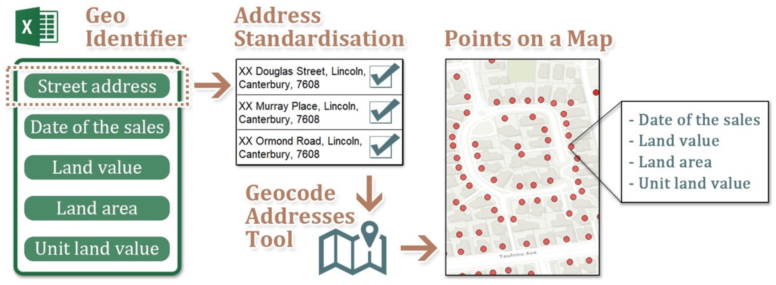
The land values are used for modelling purposes, with each of the data points subsequently adjusted to their 2021 values, accounting for inflation on a yearly basis, a technique often applied to remove the effect of inflation on price growth [34,77]. Following the adjustment, the unit land value for each sale was calculated by using the adjusted land value and the land area of the property sales. This calculation, yielding the land value per square metre, enabled a comparison of land values on a square metre rate to standardise the effect of section sizes on land value. In the next step, all the transactions were geolocated on a map by using the Geocode Addresses tool of ArcGIS Pro 3.3.1, as shown in Figure 3. The street addresses of the sales were used as an identifier for GIS geolocation.
In order to measure the level of accessibility of each property to various landscape amenities, the location and the boundaries of relevant landscape amenities were mapped using satellite maps. The selection of landscape amenity variables and the reasoning for the selection are detailed in Section 3.3. Supplementary ground-truthing was carried out in cases where satellite maps alone could not provide sufficient information for a higher mapping accuracy. To improve the validity of the model, some control variables (features or points of interest that may have potential impacts on the unit land price) were also introduced to the model. In this case, the locations and boundaries of the university campus, high school, primary school, and the closest major city, Christchurch (where many Lincoln residents commute to for work) were also included in the mapping
This mapped spatial information was then converted into numeric data for subsequent model building. This conversion involved calculating the shortest possible distance or commuting time between the location of each sale and each type of feature. It is worth noting that while ‘commuting time’ was considered a more reliable indicator of the level of accessibility, it can only be calculated when both objects are points (i.e., have a specific street address, or geo-coordinates) rather than areas indicated by GIS polygons, due to technical limitations. Therefore, the accessibility to public open spaces, water bodies, playgrounds, and sports fields was indicated by using the shortest physical distance between the location of each sale (as a point) and each type of feature (as a GIS polygon), while the accessibility to the university, schools, and Christchurch was indicated by using the shortest commuting time (i.e., the shortest travel time between two points). All the numeric data were exported and included in the hedonic model. Table 1 lists all the variables included in the model.
In addition to mapping the current (2021) status of the landscape amenities, this study also mapped the historical status of each type of amenities to capture their dynamic changes over the past 15 years (including the changes in the boundaries, construction of new amenities, and demolition of old ones) in the second stage to build temporal models and explore how the amenities’ contributions to the land values change over time. Figure 4 shows an example of how public open space, as one of the landscape amenities, has changed over time. Mapping the historical spatial status of these amenities allows this study to align sales records that occurred at each stage with the landscape amenity status at that specific time. Considering the availability interval of the historical information, this study mapped the amenities with five three-year intervals, as shown in Figure 4. The shortest possible commuting time and physical distance were also calculated using the spatial information mapped using the corresponding past status of the amenities.

3.3. Model Building

A separate model was built for each of the five three-year periods and consists of the parameters indicated in Equation (1). In the initial set of models, the land value per square metre is the dependent variable (P), while the predictor variables, listed in Table 1, were determined based on empirical reasoning due to the absence of theoretical literature for a similar geographical context. Our variable selection was informed by analogous studies conducted in different settings. In general, factors influencing land/property prices fall into four categories—S.C.L.N.: Structural attributes (i.e., building structures), Community attributes (i.e., community characteristics), Locational attributes (i.e., proximity to amenities), Neighbourhood attributes (i.e., access to services, such as schools) [78,79,80]. Given the topographical and building homogeneity of the study site, as outlined in Section 3.1, the attributes of high homogeneity were not included in the model. In the context of Lincoln township, the following variables were considered relevant, as supported by evidence in the literature: land area [81,82], distance to public open spaces [83], recreational opportunities and sport facilities [83,84], and commuting time [85]. The equation of the model is as follows:
P = α + β 1 A + β 2 D P O S + β 3 D W B + β 4 D P + β 5 D S F + β 6 T U + β 7 T H S + β 8 T P S + ε
where P is the unit land price; A is land area, DPOS is the distance to the closest public open space; DWB is the distance to the closest water body; DP is the distance to the closest playground; DSF is the distance to the closest sports field; TU is the commuting time to the university campus; THS is the commuting time to the high school campus; TPS is the commuting time to the closest primary school; β1…8 are parameters to be estimated; ε is an idiosyncratic error term. It is noteworthy that Lincoln has only one high school, one university, and two primary schools of similar popularity and parental preference. Since there is no meaningful variation in school-choice options within the township, school-related preferences were not considered a contributing factor to land-value differences in this study.
The initial set of models was tested to examine whether they meet the eight assumptions of the multiple regression models [86,87,88], as well as how each of the predictor variables contributes to the explanatory power of the model. Based on the testing results, the models underwent iterative improvement and retesting to address the issues preventing them from meeting the assumptions and improved the explanatory power by adjusting predictor variables and functional forms of the target variable and predictor variables. Given the absence of a prescribed functional form in the theoretical literature, the selection of functional forms had to be determined by empirical reasoning, as well as by comparing the goodness of fit. While the distance to the closest public open space is normally distributed, the distribution of land area shows a strong positive skewness. A reciprocal transformation is applied to convert the data to normality. Equation (2) shows the form of the final model.
P = α + β 1 A + β 2 D P O S + ε
where P is the unit land price; A is land area, DPOS is the distance to the closest public open space; β1 and β2 are parameters to be estimated; ε is an idiosyncratic error term.

4. Results and Discussion

4.1. Static Model

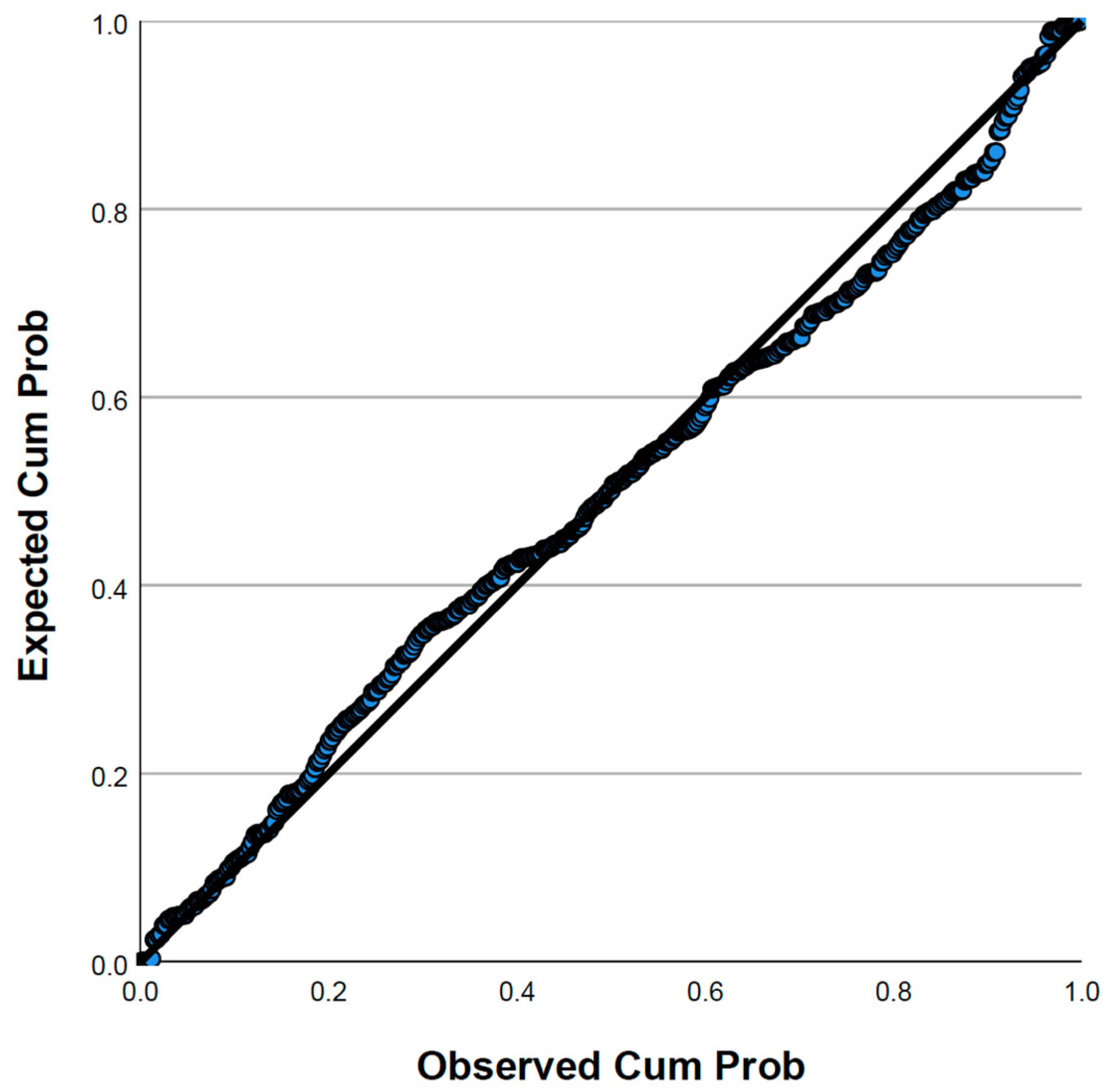
The final multiple regression model was run to predict the unit land price of real estate property sales (2019–2021) from the land area of the properties, the shortest distance between the locations of the sales, and their closest public open space. Other predictor variables were excluded from the final multiple regression models in the iterative model improvement process due to various reasons, such as multicollinearity issues and some predictor variables’ negative contribution to the explanatory power of the model. Linear relationships between the dependent variable and the inverse-transformed land area variable, as well as between the dependent variable and the shortest distance between the locations of the sales and their closest public open spaces, were observed via a visual inspection of the results. Another visual inspection of a plot of studentised residuals versus unstandardised predicted values indicates that there were homoscedasticity and a linear relationship between the target variable and the predictor variables collectively. There was independence of residuals, as assessed by a Durbin–Watson statistic of 1.770. There was no evidence of multicollinearity, as assessed by tolerance values greater than 0.1. There were no leverage values greater than 0.2 and values for Cook’s distance above 1. There are five data points whose studentised deleted residuals were greater than ±3 standard deviations but were smaller than ±3.5. Further investigations were carried out to discover any possible errors or unusual factors affecting the overall quality of the model. The assumption of normality was met, as assessed by a P-P Plot (as shown in Figure 5). The multiple regression model statistically and significantly predicted the unit land value of the sales (F(2, 391) = 1073.262, p < 0.001, adj. R2 = 0.85). Both variables added statistically significantly to the prediction (p < 0.001). Regression coefficients and standard errors can be found in Table 2.
As presented in Table 2, the multiplicative inverse of the land area exhibits a statistically significant positive impact on the unit land price. The coefficient shows that the unit land price decreases as the land area increases. This result is as expected, given that smaller land parcels are often transacted in the market at higher rates per square metre than larger land parcels. However, the relationship between the two variables is not simply linear. As the land area gradually increases, its resulting “volume discount” impact decreases and gradually approaches zero. In other words, the land price rapidly decreases with the increase in land area when the land area is small, but when the area becomes relatively large, the rate of decrease in land unit price gradually decreases and eventually infinitely approaches zero.
As exhibited in Table 2, the distance to the closest public open space is statistically significant, and as expected, negatively correlated with the unit land price. The regression coefficient of this variable suggests that the unit land price can be expected to decrease by 36.88 New Zealand Dollars with each one-kilometre increase in the distance to the closest public open space. This means that, for a typically sized residential section in Lincoln (i.e., with a median land area of 713 square metres), its total land value is expected to decrease by 2104 New Zealand Dollars for every 80 metres (or one-minute walking distance) further away from its closest public open space. The results reveal that public open space, as a typical landscape amenity, significantly contributes to the land value of residential development. It can be speculated that the land price premium is largely attributed to the landscape services provided by the public open spaces.

4.2. Temporal Model

Four similar models were built for the other four temporal periods (i.e., 2016–2018, 2013–2015, 2010–2012, and 2007–2009) following the same procedure to test the importance of public open spaces at different periods on land value. Each period is assessed individually to explore the temporal changes in the perceived value associated with an expanding urban framework and the introduction of green space. The same set of predictor variables (i.e., the land area of the properties and the closest distance from the locations of the sales to their most adjacent public open spaces) were included in the models to predict the dependent variable (i.e., the unit land price of the sales). The results of the four models are presented in Table 3 along with the model built for the period of 2019–2021. We acknowledge that these temporal delineations are a simplification. We chose a three-year span as a compromise between granularity and statistical power: shorter periods (annual, for example) might yield too few sales for reliable modelling, whereas overly long periods (five years, for example) could blur distinct phases and lower the accuracy of representing the landscape development dynamics. The 3-year intervals also correspond to the rating valuation cycles of the local district. Land values are updated every three years and therefore represent a snapshot of the value of land at a point in time and fixed for three years. The analysis was therefore also aligned with these periods to ensure consistency in the analysis. Future research might experiment with alternative segmentations (e.g., six-year periods or rolling windows) to verify the robustness of the patterns observed.
As shown in Table 3, all the models were statistically significant for predicting the unit land value of the sales. The two predictor variables (i.e., land size and the distance to the closest public open space) made a statistically significant contribution to the prediction. The correlation relationships were consistent with the model built for the 2019–2021 period presented in Section 4.1; i.e., the multiplicative inverse of the land area exhibits a significant positive impact on the unit land price, and the distance to the closest public open space has a significant negative impact on the unit land price.
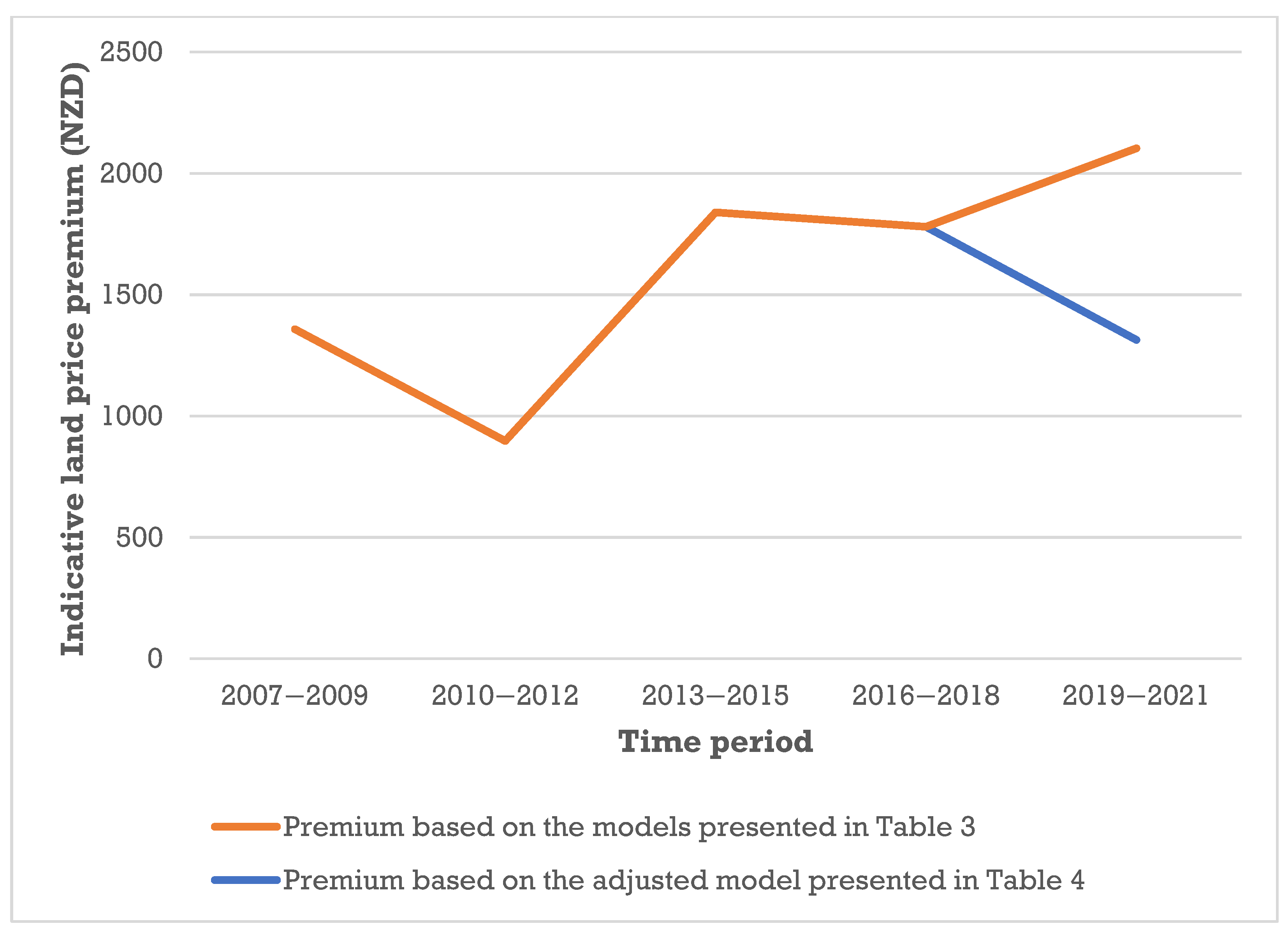
We were interested in observing the change in coefficient for open public spaces for the various periods in order to identify the effect of temporal changes on the importance of public open spaces on land value. While the impact that land size had on the sales remained very stable (with its regression coefficient remaining stable throughout the study period, as shown in Table 3), the impact that public open spaces had on the sales fluctuated, especially during 2010–2012, where the public open space coefficient is lower compared to a stable coefficient in all the other periods. By converting the regression coefficient to an indicative land price premium for the median-sized Lincoln residential property, Figure 6. visualises how the contribution of public open spaces to the sales changed over time. Apart from the period of 2010–2012, the indicative premiums for the other periods are all greater than 1300 NZD per median-sized property per one-minute walking distance (80 metres) and exhibit an increasing trend.
Interestingly, the drop in the public open space-related premium was exactly coincident with a major “black swan” event that happened during that period—The 2010/2011 Christchurch Earthquake Series caused substantial damage in Christchurch, including the loss of numerous residential properties [89,90]. Multiple neighbourhoods were impacted by soil liquefaction, and many other houses experienced structural damage. As an indication of the scale of the impact, around 8000 houses were red-zoned and demolished [91]. All of this led to a surge in property acquisitions in areas deemed to be safe and without liquefaction risk [92]. Many of these areas are located on the periphery of the city, which includes Lincoln, a town located 15 km from Christchurch [92]. When chaos hits, priorities shift [93]. The fear of missing out can drive a short-sighted market, in which securing a property can take precedence over considerations of landscape amenities. This explains the 2010–2012 drop in the open space-related premium observed in Figure 6.
A similar anomaly was observed in the data of the period 2019–2021. During data cleaning, we observed that from August 2021 onward, a large number of sales exhibited unusually rapid price increases, with some land values appearing to even double within weeks. This pattern aligns with the post-COVID economic conditions in New Zealand, characterised by the historically low mortgage interest rates and strong pent-up demand following the 2020 lockdowns [94,95]. As the impact of the post-COVID economic climate on the real-estate market only began after August 2021, the static mode presented in Table 3 and in Figure 6 (as shown by the red line) excluded the irrational sales that occurred in the four-month period between August and December 2021. This exclusion ensures that the estimated premiums reflect long-term underlying landscape-related amenity effects rather than short-term macroeconomic dynamics.
In order to examine the impacts that such “black swan” events and the resulting market boom can have on the premium of proximity to public open space, this study built another model by including the previously excluded August-December 2021 sales (n = 53). This adjusted model also statistically significantly predicted the unit land value of the sales, even if its explanatory power is lower than the original model presented previously, F(2, 444) = 174.285, p < 0.001, adj. R2 = 0.439. Both variables added statistically significantly to the prediction, p < 0.01. Regression coefficients and standard errors can be found in Table 4.
Table 4 presents several interesting facts. Firstly, it is evident that the adjusted R2 value of the adjusted model (0.44) is lower than that of the original model (0.85). This decreased adjusted R2 value indicates the lowered explanatory power of the model when the post-COVID economic climate, as an uncaptured variable, significantly influenced market sales. Secondly, while the regression coefficient of the land area variable (145,079.14) does not have a significant change (2%) in comparison to the original model (142,064.62), the coefficient of the distance to the closest public open space (−23.02) exhibits a significant difference (60%) from the original model (−36.87). This reveals that the premium related to the proximity to the public open space was significantly lowered, reducing from 2103 NZD per minute walking distance per median-sized property to 1313 NZD during a period that experienced quick house price growth and an expansionary economic climate. The trend of the open space premium of the adjusted model is shown as the blue line in Figure 6, along with the trend of the original model (shown as the red line). The difference between the two models echoes the interpretation of the premium drop in the period 2010–2012 presented earlier. In other words, both periods experienced a disruption, and the effect of this on land value reacted similarly. This decline suggests that during periods of disruption, and in particular a supply shock where supply is disrupted and demand outpaces supply, the importance of the role that landscape amenities play in the property acquisition-related decision-making process can be affected. However, another noteworthy fact is that despite the impacts of the 2010/2011 Christchurch Earthquake and COVID-19, the contribution that proximity to a public open space has had on land price has consistently been positive and statistically significant. This result underscores public open spaces’ enduring appeal to residents, to which landscape architects often contribute their value. This could also underpin how we understand landscape amenities: not just as desirable features in good times, but also as enduring assets in bad times. Furthermore, although it is not practical to eliminate the impact of the 2010/2011 Christchurch Earthquake Series on land prices, as done for the 2021 post-COVID economic climate, a reasonable inference can still be drawn based on the indications from other time periods—the premium related to the public open space is increasing over time (note: the value has been discounted to 2021 value to eliminate the impact of inflation, as detailed previously). The increasing value may be attributed to either an improved awareness of the benefits of the public open space or an improvement in the landscape quality of public open space.

4.3. Measuring the Monetary Value

In addition to revealing the association between the land price and proximity to public open space, the models can also serve as a tool for land value prediction. For example, by feeding the resulting regression coefficient values back into the predicting model, the unit land value of the period 2019–2021 can be expressed using Equation (3):
P = 104.62 + 142064.62 A 36.87 × D P O S
where P is the unit land price; A is the land area, and DPOS is the distance to the closest public open space. Since the two variables, A and DPOS, are readily available, it becomes possible to estimate the land value of a specific property using the formula. This enables the calculation of the total perceived value of a specific piece of a public open space by introducing an imaginary scenario where the target public open space is removed. The sum of land values for the land sections around the public open space (within its service catchment) can be calculated for both the actual scenario and the imaginary scenario (in which the target public open space is removed). The difference between these two sum values can then be considered an indicative value for the total perceived value of the public open space. This total perceived value can be expressed by Equation (4):
V P O S = i = 1 n 36.87 × ( D P O S A n D P O S I n ) × A n
where V P O S is the total perceived value of public open space; D P O S A n is the actual distance between the nth land section and its closest public open space; D P O S I n is the distance between the nth land section and its closest public open space in the imaginary scenario; and A n is the land area of the nth land section. We expect similar results for other “peri-urban” towns and villages that have similar landscape features. While the magnitude of the benefits might be different, this study has demonstrated the potential of this approach.
However, this paper acknowledges the limitations of this approach. Our model currently does not take into account some factors that may also influence residential land values in reality, such as the size and the quality of the public open space, landcover diversity, the proportion of private on-site green space, and scenic view quality. Although these variables are conceptually relevant, their inclusion was not feasible for methodological and data availability reasons. Firstly, as aforementioned, Lincoln’s peri-urban residential developments exhibit a high degree of homogeneity in these excluded attributes, which limits the spatial variability needed for the variables to contribute meaningfully to the model. Secondly, data availability is limited for most of these variables, whether current or historical. However, future research conducted in different geographical/temporal contexts with greater spatial variability or with access to more comprehensive datasets may be better positioned to include such variables and investigate their potential contributions to property values in greater depth.
Apart from being instrumental in aiding decision-making and communicating the value of landscape benefits, the monetary value of the public open space can also play a crucial role in supporting the planning of future residential developments. Current planning legislation in New Zealand mandates that newly built medium-density residential developments should reserve at least 20% of the entire developed site (including the area for private house plots and the shared public area) for grass or plants as landscaped areas [96]. In practice, some developers have chosen to exceed this minimum requirement, allocating more than 20% of their site to the public open space at the cost of reducing their sellable land area. This behaviour could reasonably suggest that the developers recognise that the added value generated by the presence of or the proximity to public open space may offset the reduction in sellable area and yield a better financial return overall. This appears to indicate an awareness of the relationship between proximity to green space and property value. Having an indicative monetary value for public open spaces can assist developers in identifying an optimal balance, where the overall financial return can be maximised. Also, a maximised financial return, from the residents’ perspective, equates to a maximised willingness to pay, reflecting the maximised values that landscapes can offer, which are not limited to economic benefits, but rather also include environmental, social, and cultural benefits.
Our analysis also prompts reflection on its implications for equity—if living near an open space adds significant value, there is a risk that such amenities become more accessible for higher-income residents who can afford the premium, and planning new public open spaces in less affluent communities might unintentionally contribute to gentrification pressures. These socio-spatial inequalities are central to broader concerns about environmental justice. Recognising this dynamic, planners and policymakers might need to take into account both the public open space premium and its associated environmental justice concerns. Essentially, the “universal currency” we discuss has an ethical dimension: it quantifies value but does not in itself guarantee fair access to that value. Currently, within Lincoln, this dynamic may not yet be an issue requiring immediate attention, as the town is small and most residents live relatively close to some form of open space. However, in larger urban areas, the implications could be much more significant.
While the hedonic model developed in this study effectively quantified the perceived value of public open space in Lincoln, its generalisability to other geographical contexts should be approached with caution. The fast-growing peri-urban context of Lincoln, combined with its relatively homogeneous spatial attributes, differs from the conditions of some other geographical contexts, such as larger metropolitan centres, which normally have a high variability in spatial attributes. However, while the magnitude of the identified premiums may not be directly translatable to other contexts, the modelling framework itself is transferable. With locally relevant spatial datasets and amenity characteristics, this approach can be adapted for application in settings with different market dynamics, demographic compositions, or planning frameworks. Further testing of this “universal currency” in other contexts would help evaluate its robustness and broader applicability as well.

5. Conclusions

This study explores the potential of using the hedonic model approach to measure the value of perceived landscape benefits, which are often intangible and difficult to quantify. By translating the perceived benefits into monetary value, such intangible benefits can become comparable to tangible landscape benefits. Also, by incorporating other monetised tangible benefits (which are often quantified through market transaction prices), it becomes possible to calculate an overall value for a specific landscape, enabling comparison between landscape benefits and their associated costs. Through this preliminary exploration of quantifying the intangible benefits of public open spaces, we also demonstrate the potential of using a revealed preference approach to quantify the perceived values of landscape benefits. Such values can serve as a “universal currency” for bridging gaps between different landscape performance measurements.
Through the employment of the hedonic pricing approach, this study not only establishes a predictive model revealing how proximity to public open space—a prominent type of landscape amenity providing diverse benefits—affects the land price but also examines the temporal variations in the land price premium related to the proximity to public open space.
The model for the latest research period reveals a nonlinear decrease in unit land price with increasing land area. Also, proximity to public open spaces, as another significant factor, was found to positively contribute to the unit land price.
The temporal analysis spanning 15 years, while demonstrating the impacts that unforeseen events can have on the public open space-related land price premium, also indicates that public open spaces have always been a positive factor influencing the land price, and the influence has always been statistically significant.
However, it is important to acknowledge that this study represents only a preliminary exploration within a broader effort to address the identified challenges in Landscape Performance Evaluations. While our findings suggest that adapting economic approaches and using monetary value as a “universal currency” is a promising direction for addressing the disconnection between different landscape benefit measurements and between costs and benefits, future research is required to meet the goal of bridging the measurement gaps. From an LPE perspective, our study contributes a piece of the puzzle needed to address the two key challenges identified by prior research: comparing different benefits and linking benefits to costs. We showed that it is feasible to express at least one group of landscape benefits (related to open space access) in the same unit as costs (i.e., monetary terms). This is a step toward enabling cost–benefit analyses that were previously hampered by incompatible units. If, for instance, a new park costs $X to build and maintain, and our model indicates it adds $Y in land value premium to surrounding properties, decision-makers have a tangible way to weigh those numbers. However, we reaffirm that our aim is not to argue that monetary measures capture all that matters in landscapes. Instead, by providing a “universal currency”, we hope to equip planners and decision makers with a tool to argue for the contributions landscape interventions can have on human wellbeing. Yet, as with any tool, it must be used judiciously—complemented by considerations of various dimensions that might not have direct market analogues and not be reflected by goods in the market.
Our results reveal promising avenues for future research to assess how landscape benefits introduced in new residential subdivision developments generate value for the users of these areas. Further exploration using spatial models such as spatial lag models, spatial error models, or weighted geographic models can help assess how location-specific landscape features influence land values. Since our study did not run a spatial econometric model, spatial dependence and heterogeneity in the data that have not been accounted for might have an impact on the analysis.
A promising direction for future exploration is using the multiple regression models built in a specific context to predict the add-on value offered by certain types of landscape features. When combined with cost estimation, these models can provide valuable evidence for supporting decision-making in landscape planning and development. Such approaches can also be applied retrospectively to estimate the perceived value of existing landscape features, offering insights into their contributions to improved landscape benefits.
Another critical area for further investigation is the development of a landscape benefit value structure/framework. A well-defined value structure/framework would help prevent overlaps or omissions in value calculations, ensuring more precise alignment between monetisation methods and the scope of benefits, either in the form of individual benefits, or in other cases, more practically, in the form of well-defined value groups. Such well-defined value structures/frameworks and clear alignment would then allow inter-benefit comparisons, as well as more robust cost–benefit analyses.
We also acknowledge that landscapes are inherently complex systems, with their overall performance shaped by many small factors that are often dynamic and interrelated. Due to technical and resource constraints, this study was unable to fully capture these subtleties. Highlighting these limitations is crucial for future research, which we believe may benefit from the availability of a broader range of data and techniques, enabling deeper and more comprehensive exploration of the contributions that various factors have on the value of landscapes.
In essence, this research not only enhances the understanding of the perceived values of public open space but also provides a practical tool for stakeholders or decision-makers in assisting their planning process. By acknowledging the enduring positive impact of public open spaces on land prices, even when facing external disruptions, this study underscores the importance of landscape amenities in shaping human well-being.

Author Contributions

Conceptualisation, G.C., D.D., S.D. and J.B.; methodology G.C., D.D., S.D. and J.B.; software, G.C.; formal analysis, G.C. and D.D.; investigation, G.C.; data curation, G.C. and D.D.; writing—original draft preparation, G.C.; writing—review and editing, G.C., D.D., S.D. and J.B.; visualisation, G.C.; supervision, D.D., S.D. and J.B. All authors have read and agreed to the published version of the manuscript.

Funding

This research received no external funding.

Institutional Review Board Statement

Not applicable.

Informed Consent Statement

Not applicable.

Data Availability Statement

The data used for this research were obtained from a proprietor and are therefore not publicly available. Any queries can be directed to the corresponding author, and the data may be made available on request.

Conflicts of Interest

The authors declare no conflicts of interest.

Abbreviations

The following abbreviations are used in this manuscript:
CBDCentral Business District
CSICase Study Investigation
GISsGeographical Information Systems
LAFLandscape Architecture Foundation
LPELandscape Performance Evaluation

References

  1. Bell, S.; Sarlöv Herlin, I.; Stiles, R. Exploring the Boundaries of Landscape Architecture; Routledge: New York, NY, USA, 2012. [Google Scholar]
  2. Egoz, S. Landscape Is More Than the Sum of Its Parts: Teaching an Understanding of Landscape Complexity, 1st ed.; Routledge: London, UK, 2019; pp. 84–95. [Google Scholar]
  3. Swaffield, S.; Deming, M.E. Research strategies in landscape architecture: Mapping the terrain. J. Landsc. Archit. 2011, 6, 34–45. [Google Scholar] [CrossRef]
  4. Deming, M.E.; Swaffield, S. Landscape Architecture Research: Inquiry, Strategy, Design; John Wiley & Sons, Inc.: Hoboken, NJ, USA, 2011. [Google Scholar]
  5. Howard, P.; Thompson, I.; Waterton, E.; Atha, M. The Routledge Companion to Landscape Studies, 2nd ed.; Routledge: London, UK, 2019. [Google Scholar]
  6. Thompson, I.H. Landscape Architecture: A Very Short Introduction; Oxford University Press: Oxford, UK, 2014. [Google Scholar]
  7. Barnes, M. Evaluating Landscape Performance; Landscape Architecture Foundation: Washington, DC, USA, 2019. [Google Scholar]
  8. Landscape Architecture Foundation. About Landscape Performance. Available online: https://www.landscapeperformance.org/about-landscape-performance (accessed on 19 October 2023).
  9. Landscape Architecture Foundation. Landscape Performance Series Turns 10. Available online: https://www.landscapeperformance.org/blog/2020/09/landscape-performance-turns-10 (accessed on 1 October 2025).
  10. Niland, J. Landscape Architecture Is Now Officially a STEM Discipline. Available online: https://archinect.com/news/article/150356461/landscape-architecture-is-now-officially-a-stem-discipline-according-to-the-u-s-department-of-homeland-security (accessed on 1 October 2025).
  11. Landscape Architecture Foundation. Keeping Promises: Exploring the Role of Post-Occupancy Evaluation in Landscape Architecture. Available online: https://www.landscapeperformance.org/blog/2014/11/role-of-poe (accessed on 23 September 2021).
  12. Chen, G.; Bowring, J.; Davis, S. Measuring the Performance of the Built Environment: An Investigation of Evaluation Methods. Urban Sci. 2025, 9, 536. [Google Scholar] [CrossRef]
  13. Yang, B. Landscape performance evaluation in socio-ecological practice: Current status and prospects. Socio-Ecol. Pract. Res. 2020, 2, 91–104. [Google Scholar] [CrossRef]
  14. Yang, B.; Li, S.; Binder, C. A research frontier in landscape architecture: Landscape performance and assessment of social benefits. Landsc. Res. 2016, 41, 314–329. [Google Scholar] [CrossRef]
  15. Ozdil, T.R. Social value of urban landscapes: Performance study lessons from two iconic Texas projects. Landsc. Archit. Front. 2016, 4, 12–30. [Google Scholar]
  16. Chen, G.; Bowring, J.; Davis, S. Performance evaluation: Identifying barriers and enablers for landscape architecture practice. Architecture 2021, 1, 140–160. [Google Scholar] [CrossRef]
  17. De Montis, A. Measuring the performance of planning: The conformance of Italian landscape planning practices with the European Landscape Convention. Eur. Plan. Stud. 2016, 24, 1727–1745. [Google Scholar] [CrossRef]
  18. Wende, W. Landscape planning and ecosystem services in Europe and beyond. Ecosyst. People 2019, 15, 347–350. [Google Scholar] [CrossRef]
  19. Corkery, L. Connecting Research with Practice to Assess Landscape Performance. Landsc. Rev. 2024, 20, 27–38. [Google Scholar] [CrossRef]
  20. Chen, G.; Bowring, J.; Davis, S. How is “success” defined and evaluated in landscape architecture: A collective case study of landscape architecture performance evaluation approaches in New Zealand. Sustainability 2023, 15, 15162. [Google Scholar] [CrossRef]
  21. Chen, G.; Bowring, J.; Davis, S. Exploring the terminology, definitions, and forms of Post-Occupancy Evaluation (POE) in landscape architecture. Land 2023, 12, 882. [Google Scholar] [CrossRef]
  22. Bowring, J.; Chen, G. Te Whāriki Subdivision Phases 1 and 2 methods. In Landscape Performance Series; Landscape Architecture Foundation: Washington, DC, USA, 2022. [Google Scholar]
  23. Chen, G.; Bowring, J. Measuring landscape performance for a subdivision in Canterbury, New Zealand: Reflections and critique of methods. In Proceedings of the CELA 2022 Annual Conference, Evolving Norms: Adapting Scholarship to Disruptive Phenomena, Santa Ana Pueblo, NM, USA, 16–19 March 2022. [Google Scholar]
  24. Etter, H.; Schwedes, S.; Hebbrecht, J. Environmental Economics and Ecosystem Valuation—The Rationale Behind; ELD Initiative: Bonn, Germany, 2019. [Google Scholar]
  25. Munns, W.R., Jr.; Rea, A.W. Ecosystem services: Value is in the eye of the beholder. Integr. Environ. Assess. Manag. 2015, 11, 332–333. [Google Scholar] [CrossRef]
  26. Pannell, D.J.; Roberts, A.M.; Park, G.; Alexander, J. Designing a practical and rigorous framework for comprehensive evaluation and prioritisation of environmental projects. Wildl. Res. 2013, 40, 126–133. [Google Scholar] [CrossRef]
  27. Chen, G.; Bowring, J.; Davis, S. Why landscape architects should embrace landscape performance evaluation—The “market” perspective of landscape development. Landsc. Rev. 2024, 20, 61–67. [Google Scholar] [CrossRef]
  28. Luttik, J. The value of trees, water and open space as reflected by house prices in the Netherlands. Landsc. Urban Plan. 2000, 48, 161–167. [Google Scholar] [CrossRef]
  29. Tyrväinen, L. The amenity value of the urban forest: An application of the hedonic pricing method. Landsc. Urban Plan. 1997, 37, 211–222. [Google Scholar] [CrossRef]
  30. Chaparro, L.; Terradas, J. Ecological Services of Urban Forest in Barcelona; Institut Municipal de Parcs i Jardins Ajuntament de Barcelona, Àrea de Medi Ambient: Barcelona, Spain, 2009. [Google Scholar]
  31. McPherson, E.G.; Simpson, J.R.; Peper, P.J.; Xiao, Q. Benefit-Cost Analysis of Modesto’s Municipal Urban Forest. Arboric. Urban For. (AUF) 1999, 25, 235. [Google Scholar] [CrossRef]
  32. Xiao, Q.; McPherson, E.G.; Simpson, J.; Ustin, S. Rainfall Interception by Sacramento’s Urban Forest. Arboric. Urban For. (AUF) 1998, 24, 235. [Google Scholar] [CrossRef]
  33. Morancho, A.B. A hedonic valuation of urban green areas. Landsc. Urban Plan. 2003, 66, 35–41. [Google Scholar] [CrossRef]
  34. Ludick, A.; Dyason, D.; Fourie, A. A new affordable housing development and the adjacent housing-market response. S. Afr. J. Econ. Manag. Sci. 2021, 24, a3637. [Google Scholar] [CrossRef]
  35. Davidson, N.C.; van Dam, A.A.; Finlayson, C.M.; McInnes, R.J. Worth of wetlands: Revised global monetary values of coastal and inland wetland ecosystem services. Mar. Freshw. Res. 2019, 70, 1189–1194. [Google Scholar] [CrossRef]
  36. Fernandez, M.A. Better Together? Wetlands, Parks and Housing Prices in Auckland; Auckland Council, Te Kaunihera o Tāmaki Makaurau: Auckland, New Zealand, 2020. [Google Scholar]
  37. Cohen, J.P.; Cromley, R.G.; Banach, K.T. Are Homes Near Water Bodies and Wetlands Worth More or Less? An Analysis of Housing Prices in One Connecticut Town. Growth Change 2015, 46, 114–132. [Google Scholar] [CrossRef]
  38. Du, X.; Huang, Z. Spatial and temporal effects of urban wetlands on housing prices: Evidence from Hangzhou, China. Land Use Policy 2018, 73, 290–298. [Google Scholar] [CrossRef]
  39. Tapsuwan, S.; Ingram, G.; Burton, M.; Brennan, D. Capitalized amenity value of urban wetlands: A hedonic property price approach to urban wetlands in Perth, Western Australia*. Aust. J. Agric. Resour. Econ. 2009, 53, 527–545. [Google Scholar] [CrossRef]
  40. Gopalakrishnan, S.; Smith, M.D.; Slott, J.M.; Murray, A.B. The value of disappearing beaches: A hedonic pricing model with endogenous beach width. J. Environ. Econ. Manag. 2011, 61, 297–310. [Google Scholar] [CrossRef]
  41. Fraser, R.; Spencer, G. The Value of an Ocean View: An Example of Hedonic Property Amenity Valuation. Aust. Geogr. Stud. 1998, 36, 94–98. [Google Scholar] [CrossRef]
  42. Nicholls, S.; Crompton, J.L. The contribution of scenic views of, and proximity to, lakes and reservoirs to property values. Lakes Reserv. Sci. Policy Manag. Sustain. Use 2018, 23, 63–78. [Google Scholar] [CrossRef]
  43. Klizentyte, K.; Susaeta, A.; Adams, D.C.; Stein, T.V. Recreation Area Characteristics and Their Impact on Property Values within Florida’s Wekiva River System. Soc. Nat. Resour. 2024, 37, 48–72. [Google Scholar] [CrossRef]
  44. Brandt, S.; Maennig, W. Road noise exposure and residential property prices: Evidence from Hamburg. Transp. Res. Part D Transp. Environ. 2011, 16, 23–30. [Google Scholar] [CrossRef]
  45. Clark, D.E.; Herrin, W.E. The Impact of Public School Attributes on Home Sale Prices in California. Growth Change 2000, 31, 385–407. [Google Scholar] [CrossRef]
  46. McPherson, E.G.; Nowak, D.; Heisler, G.; Grimmond, S.; Souch, C.; Grant, R.; Rowntree, R. Quantifying urban forest structure, function, and value: The Chicago Urban Forest Climate Project. Urban Ecosyst. 1997, 1, 49–61. [Google Scholar] [CrossRef]
  47. Klaus, I.S.; McPherson, E.G.; James, R.S. Air Pollutant Uptake by Sacramento’s Urban Forest. Arboric. Urban For. (AUF) 1998, 24, 224. [Google Scholar] [CrossRef]
  48. Nowak, D.J.; Hoehn, R.E.; Crane, D.E.; Stevens, J.C.; Walton, J.T. Assessing Urban Forest Effects and Values: Philadelphia’s Urban Forest; US Department of Agriculture, Forest Service, Northern Research Station: Washington, DC, USA, 2007.
  49. Zabel, J.E.; Kiel, K.A. Estimating the Demand for Air Quality in Four U.S. Cities. Land Econ. 2000, 76, 174–194. [Google Scholar] [CrossRef]
  50. Simpson, J.R. Urban forest impacts on regional cooling and heating energy use: Sacramento County case study. J. Arboric. 1998, 24, 201–214. [Google Scholar] [CrossRef]
  51. Bolund, P.; Hunhammar, S. Ecosystem services in urban areas. Ecol. Econ. 1999, 29, 293–301. [Google Scholar] [CrossRef]
  52. Nowak, D.J.; Crane, D.E. Carbon storage and sequestration by urban trees in the USA. Environ. Pollut. 2002, 116, 381–389. [Google Scholar] [CrossRef]
  53. Chan, K.M.A.; Satterfield, T.; Goldstein, J. Rethinking ecosystem services to better address and navigate cultural values. Ecol. Econ. 2012, 74, 8–18. [Google Scholar] [CrossRef]
  54. Millennium Ecosystem Assessment. Ecosystems and Human Well-Being; World Health Organization: Geneva, Switzerland, 2005.
  55. de Groot, R.S.; Wilson, M.A.; Boumans, R.M.J. A typology for the classification, description and valuation of ecosystem functions, goods and services. Ecol. Econ. 2002, 41, 393–408. [Google Scholar] [CrossRef]
  56. Canfield, J.; Yang, B.; Whitlow, H. Evaluating Landscape Performance—A Guidebook for Metrics and Methods Selection; Landscape Architecture Foundation: Washington, DC, USA, 2018. [Google Scholar]
  57. Candelaria, J.L.; Sharifi, A.; Simangan, D.; Tabosa, R.M.R. A critical analysis of selected global sustainability assessment frameworks: Toward integrated approaches to peace and sustainability. World Dev. Perspect. 2023, 32, 100539. [Google Scholar] [CrossRef]
  58. O’Connor, M. The “Four Spheres” framework for sustainability. Ecol. Complex. 2006, 3, 285–292. [Google Scholar] [CrossRef]
  59. Deming, M.E. Social & cultural metrics: Measuring the intangible benefits of designed landscapes. Landsc. Archit. 2015, 1, 99–109. [Google Scholar]
  60. Gibbons, S.; Mourato, S.; Resende, G.M. The Amenity Value of English Nature: A Hedonic Price Approach. Environ. Resour. Econ. 2014, 57, 175–196. [Google Scholar] [CrossRef]
  61. Fan, Q.; Hansz, J.A.; Yang, X. The Pricing Effects of Open Space Amenities. J. Real Estate Financ. Econ. 2016, 52, 244–271. [Google Scholar] [CrossRef]
  62. Córdoba Hernández, R.; Camerin, F. The application of ecosystem assessments in land use planning: A case study for supporting decisions toward ecosystem protection. Futures 2024, 161, 103399. [Google Scholar] [CrossRef]
  63. McCauley, D.J. Selling out on nature. Nature 2006, 443, 27–28. [Google Scholar] [CrossRef]
  64. Kerr, G.N.; Greer, G. New Zealand River Management: Economic Values of Rangitata River Fishery Protection. Australas. J. Environ. Manag. 2004, 11, 139–149. [Google Scholar] [CrossRef]
  65. Carson, R.T.; Mitchell, R.C.; Hanemann, M.; Kopp, R.J.; Presser, S.; Ruud, P.A. Contingent Valuation and Lost Passive Use: Damages from the Exxon Valdez Oil Spill. Environ. Resour. Econ. 2003, 25, 257–286. [Google Scholar] [CrossRef]
  66. Sheppard, R.; Kerr, G.N.; Tipler, C.; Cullen, R.; Ferguson, T. Recreational Water Quality Standards for the Waimakariri River. Report to Canterbury Regional Council; AERU, Lincoln University: Lincoln, New Zealand, 1992. [Google Scholar]
  67. New Zealand Transport Agency Waka Kotahi. Monetised Benefits and Costs Manual; New Zealand Transport Agency: Wellington, New Zealand, 2025. [Google Scholar]
  68. Ministry of Transport (MoT). Social Cost of Road Crashes and Injuries; Ministry of Transport: Wellington, New Zealand, 2017.
  69. Clough, P.; Bealing, M. What’s the Use of Non-Use Values? Non-Use Values and the Investment Statement; NZ Institute of Economic Research: Wellington, New Zealand, 2018. [Google Scholar]
  70. Boyle, K.J. Introduction to Revealed Preference Methods. In A Primer on Nonmarket Valuation; Champ, P.A., Boyle, K.J., Brown, T.C., Eds.; Springer Netherlands: Dordrecht, The Netherlands, 2003; pp. 259–267. [Google Scholar]
  71. Bockstael, N.E.; McConnell, K.E. Environmental and Resource Valuation with Revealed Preferences: A Theoretical Guide to Empirical Models; Springer Science & Business Media: New York, NY, USA, 2007; Volume 7. [Google Scholar]
  72. Montero, J.-M.; Fernández-Avilés, G. Hedonic Price Model. In Encyclopedia of Quality of Life and Well-Being Research; Michalos, A.C., Ed.; Springer: Dordrecht, The Netherlands, 2014; pp. 2834–2837. [Google Scholar]
  73. Taylor, L.O. The hedonic method. In A Primer on Nonmarket Valuation; Champ, P.A., Boyle, K.J., Brown, T.C., Eds.; Springer: Berlin/Heidelberg, Germany, 2003; pp. 331–393. [Google Scholar]
  74. Baker, R.; Ruting, B. Environmental Policy Analysis: A Guide to Non-Market Valuation; Productivity Commission Staff Working Paper; Productivity Commission: Canberra, Australia, 2014. [Google Scholar]
  75. Statistics New Zealand. Subnational Population Estimates (RC, SA2), by Age and Sex, at 30 June 1996–2023 (2023 Boundaries); Statistics New Zealand: Wellington, New Zealand, 2023. [Google Scholar]
  76. Headway Systems. Headway Systems: Bringing Value to the Property Industry. Available online: https://headway.co.nz/valbiz-v8/ (accessed on 16 February 2025).
  77. Acharya, A.; Basu, S.; Hanink, D.M. Spatial Hedonic Regression Analysis of the Impact of Cell Towers on Las Vegas Real Estate Market. Prof. Geogr. 2022, 74, 715–726. [Google Scholar] [CrossRef]
  78. Yan, S.; Delmelle, E.; Duncan, M. The impact of a new light rail system on single-family property values in Charlotte, North Carolina. J. Transp. Land Use 2012, 5, 60–67. [Google Scholar] [CrossRef]
  79. Aziz, A.; Anwar, M.M.; Dawood, M. The impact of neighborhood services on land values: An estimation through the hedonic pricing model. GeoJournal 2021, 86, 1915–1925. [Google Scholar] [CrossRef]
  80. Thiwanka, A.; Wickramaarachchi, N. Critical Determinants of Residential Land Values in a Suburban Area: A Perception Analysis. Sri Lankan J. Real Estate 2022, 1, 61. [Google Scholar] [CrossRef]
  81. Helbich, M.; Brunauer, W.; Vaz, E.; Nijkamp, P. Spatial heterogeneity in hedonic house price models: The case of Austria. Urban Stud. 2014, 51, 390–411. [Google Scholar] [CrossRef]
  82. Ottensmann, J.R.; Payton, S.; Man, J. Urban location and housing prices within a hedonic model. J. Reg. Anal. Policy 2008, 38, 19–35. [Google Scholar] [CrossRef]
  83. Crompton, J.L.; Nicholls, S. Impact on property values of distance to parks and open spaces: An update of U.S. studies in the new millennium. J. Leis. Res. 2020, 51, 127–146. [Google Scholar] [CrossRef]
  84. Russell, S.; Kweon, B.-S. The Economic Effect of Parks and Community-Managed Open Spaces on Residential House Prices in Baltimore, MD. Land 2025, 14, 483. [Google Scholar] [CrossRef]
  85. Metz, N. Effect of distance to schooling on home prices. Rev. Reg. Stud. 2015, 45, 151. [Google Scholar] [CrossRef]
  86. Berry, W.D. Understanding Regression Assumptions; Sage: Newbury Park, CA, USA, 1993. [Google Scholar]
  87. Lewis-Beck, C.; Lewis-Beck, M. Applied Regression: An Introduction; Sage Publications: Thousand Oaks, CA, USA, 2016. [Google Scholar]
  88. Wiley, J. Applied Linear Regression, 4th ed.; Wiley: New York, NY, USA, 2014. [Google Scholar]
  89. Potter, S.H.; Becker, J.S.; Johnston, D.M.; Rossiter, K.P. An overview of the impacts of the 2010-2011 Canterbury earthquakes. Int. J. Disaster Risk Reduct. 2015, 14, 6–14. [Google Scholar] [CrossRef]
  90. Dyason, D. Disasters and investment: Assessing the performance of the underlying economy following a large-scale stimulus in the built environment. J. Risk Financ. Manag. 2022, 15, 263. [Google Scholar] [CrossRef]
  91. Canterbury Earthquake Recovery Authority. Land Zoning Policy and the Residential Red Zone: Responding to Land Damage and Risk to Life; Canterbury Earthquake Recovery Authority: Wellington, New Zealand, 2016. [Google Scholar]
  92. Brunsdon, N. Christchurch Goes Up and Out. Available online: https://www.buildmagazine.org.nz/assets/PDF/Build-172-73-Feature-Canterbury-Today-Christchurch-Goes-Up-And-Out.pdf (accessed on 30 October 2025).
  93. Hodkinson, C. ‘Fear of Missing Out’ (FOMO) marketing appeals: A conceptual model. J. Mark. Commun. 2019, 25, 65–88. [Google Scholar] [CrossRef]
  94. Yiu, C.Y. Why House Prices Increase in the COVID-19 Recession: A Five-Country Empirical Study on the Real Interest Rate Hypothesis. Urban Sci. 2021, 5, 77. [Google Scholar] [CrossRef]
  95. Chadwick, M.; Nahavandi, A. How Does Monetary Policy Affect the New Zealand Housing Market Through the Credit Channel? Reserve Bank of New Zealand: Wellington, New Zealand, 2022. [Google Scholar]
  96. Ministry for the Environment. Understanding the Resource Management (Enabling Housing Supply and Other Matters) Amendment Act 2021: Medium Density Residential Standards—A Guide for Territorial Authorities; Ministry for the Environment: Wellington, New Zealand, 2022.
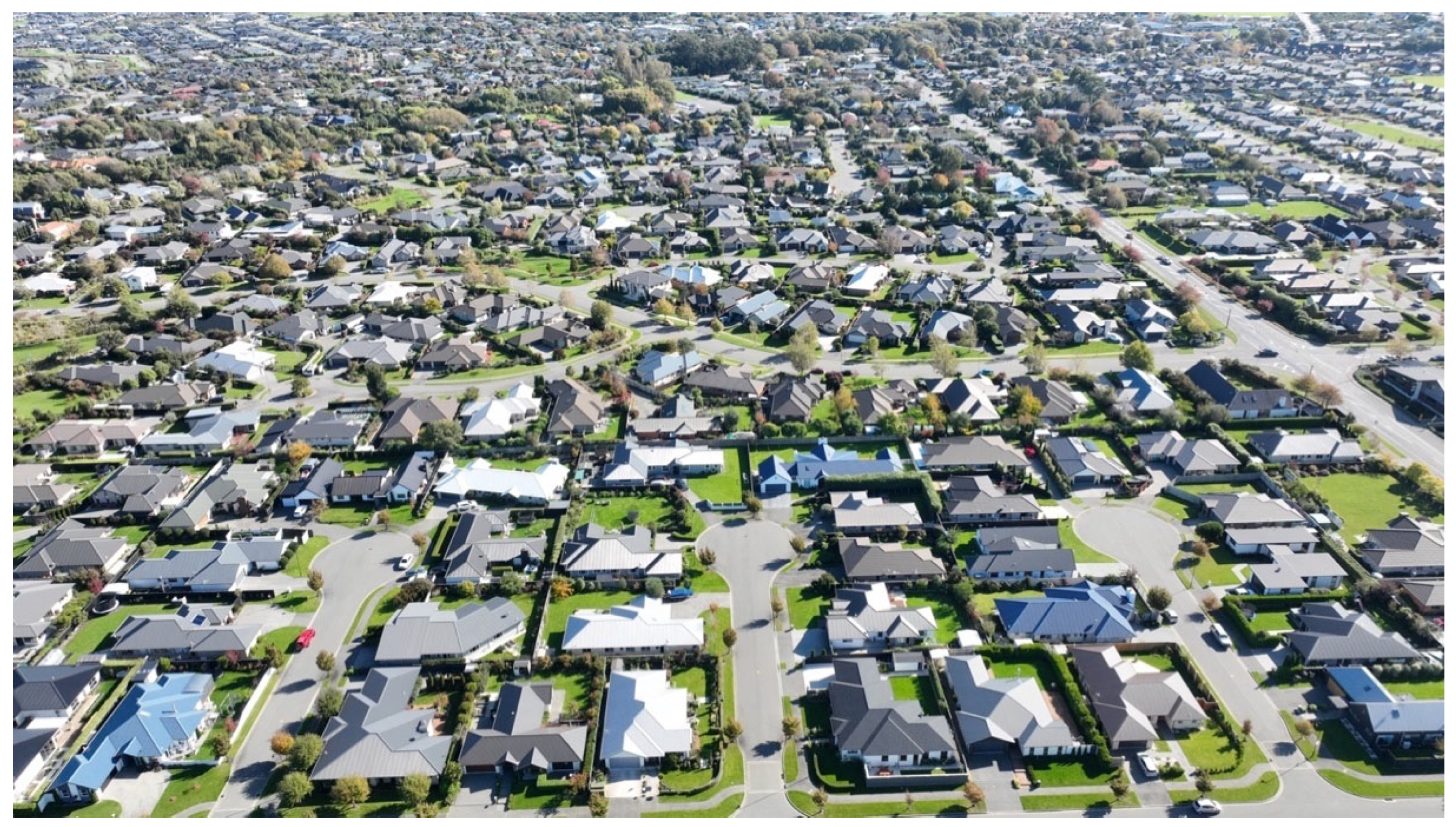
Figure 2. A drone image looking Northwest across Lincoln township from the air (Image credit: Donald Royds, 2023).
Urbansci 10 00007 g002
Figure 3. Geolocating the sales on a map. Source: Authors’ work, 2025.
Urbansci 10 00007 g003
Figure 4. The spatial status of the public open space changes over time during the 15-year study period. The green overlays on the satellite imagery indicate the configuration of public open space at the times shown above each map. Source: Authors’ work, 2025.
Urbansci 10 00007 g004
Figure 5. Normal P-P plot of regression standardised residual. Authors’ work, 2025.
Urbansci 10 00007 g005
Figure 6. Indicative land price premium (for a typically sized Lincoln residential property) contributed by getting 80-metre (one-minute walking distance) closer to a public open space (NZD). Source: Authors’ calculations, 2025.
Urbansci 10 00007 g006
Table 1. List of variables included in the model.
VariablesUnit
IdentifiersStreet address/
Date of the saleYear-Month-Date
Target variableUnit land valueNew Zealand dollar/sqm
Predictor variableDistance to the closest public open spaceMetre
Distance to the closest water bodyMetre
Distance to the closest playgroundMetre
Distance to the closest sports fieldMetre
Commuting time to the university campusMinute
Commuting time to the high school campusMinute
Commuting time to the closest primary schoolMinute
Land areaSquare metre
Table 2. Multiple regression results for Unit Land Price (2019–2021).
Unit Land PriceB95% CI for BSE BβR2R2
LLUL
Model 0.850.85 ***
   Constant104.62 ***95.01114.234.89
   Land area_Inverse142,064.62 ***135,670.73148,458.513252.070.89 ***
   Distance to the closest public open space−36.87 ***−47.63−26.125.47−0.14 ***
Note. B = unstandardised regression coefficient; CI = confidence interval; LL = lower limit; UL = upper limit; SE B = standard error of the coefficient; β = standardised coefficient; R2 = coefficient of determination; ∆R2 = adjusted R2. *** p < 0.001.
Table 3. Multiple regression results of the temporal models for Unit Land Price.
Model 1Model 2Model 3Model 4The Static Model
Temporal Period (2007–2009)(2010–2012)(2013–2015)(2016–2018)(2019–2021)
ModelR20.85 ***0.74 ***0.80 ***0.85 ***0.85 ***
R20.85 ***0.73 ***0.80 ***0.85 ***0.85 ***
ConstantB121.66 ***107.44 ***100.50 ***105.05 ***104.62 ***
Land area_InverseB153,799.66 ***149,453.08 ***143,968.53 ***136,705.59 ***142,064.62 ***
Distance to the closest public open spaceB−23.81 ***−15.73 ***−32.25 ***−31.20 ***−36.87 ***
Note. Model = “Enter” method in SPSS Statistics 29; B = unstandardised regression coefficient; R2 = coefficient of determination; ∆R2 = adjusted R2. *** p < 0.001.
Table 4. Adjusted multiple regression results for Unit Land Price.
Unit Land PriceB95% CI for BSE BβR2R2
LLUL
Model 0.440.44 ***
   Constant108.15 ***83.82132.4712.38
   Land area_Inverse145,079.14 ***128,649.62161,508.668359.560.63 ***
   Distance to the closest public open space−23.02 **−38.16−7.897.70−0.11 **
Note. Model = “Enter” method in SPSS Statistics 29; B = unstandardised regression coefficient; CI = confidence interval; LL = lower limit; UL = upper limit; SE B = standard error of the coefficient; β = standardised coefficient; R2 = coefficient of determination; ∆R2 = adjusted R2. ** p < 0.01. *** p < 0.001.
Disclaimer/Publisher’s Note: The statements, opinions and data contained in all publications are solely those of the individual author(s) and contributor(s) and not of MDPI and/or the editor(s). MDPI and/or the editor(s) disclaim responsibility for any injury to people or property resulting from any ideas, methods, instructions or products referred to in the content.