Abstract
Human-sourced emissions of carbon dioxide (CO2) into the Earth’s atmosphere have been implicated in contemporary global warming, based mainly on computer modeling. Growing empirical evidence reviewed here supports the alternative hypothesis that global climate change is governed primarily by a natural climate cycle, the Antarctic Oscillation. This powerful pressure-wind-temperature cycle is energized in the Southern Ocean and teleconnects worldwide to cause global multidecadal warm periods like the present, each followed historically by a multidecadal cold period, which now appears imminent. The Antarctic Oscillation is modulated on a thousand-year schedule to create longer climate cycles, including the Medieval Warm Period and Little Ice Age, which are coupled with the rise and fall, respectively, of human civilizations. Future projection of these ancient climate rhythms enables long-term empirical climate forecasting. Although human-sourced CO2 emissions play little role in climate change, they pose an existential threat to global biodiversity. Past mass extinctions were caused by natural CO2 surges that acidified the ocean, killed oxygen-producing plankton, and induced global suffocation. Current human-sourced CO2 emissions are comparable in volume but hundreds of thousands of times faster. Diverse evidence suggests that the consequent ocean acidification is destroying contemporary marine phytoplankton, corals, and calcifying algae. The resulting global oxygen deprivation could smother higher life forms, including people, by 2100 unless net human-induced CO2 emissions into the atmosphere are ended urgently.
1. Introduction and Overview
The current geologic period has been termed the “Anthropocene” in recognition of the dominant human influence on global geophysical and biological systems and cycles [1,2,3,4,5,6,7,8,9]. The term is debated [10,11,12] and remains unofficial [9], but there is no disagreement that humans have significantly impacted the natural world. These impacts can be positive, negative, or both [13]. Two such negative impacts are considered potentially high risk and even threatening to life on Earth: global warming (United Nations (UN) Intergovernmental Panel on Climate Change (IPCC) [14,15,16,17,18,19,20,21,22] and biodiversity loss caused by ocean acidification (OA) [23], which is contributing to the ongoing human-induced “Sixth Mass Extinction” (SME) [23,24,25,26,27,28,29,30,31,32].
Climate change and biodiversity loss are arguably the two greatest environmental challenges of the Anthropocene. The two risks are connected by carbon dioxide (CO2), which has been implicated in both. This review addresses climate and biodiversity by integrating empirical evidence from diverse interdisciplinary sources to address a crucial question about each: what is the relative contribution of human versus (vs.) natural influence? If human influences predominate, mitigation of adverse effects may be possible by modifying collective societal behavior through policy. If natural processes prevail, adaptation to potential adverse effects may be the only option, since the underlying natural processes may be immune to deliberate human intervention and any such attempts may provoke unintended adverse consequences. In either case, answers to this guiding question inform new risk assessments with broad ramifications for policy and law at all jurisdictional levels and potentially decisive implications for continued life on Earth.
In climate science, the prevailing paradigm has been that humans cause contemporary global warming by emitting CO2 into the air from burning fossil fuels and deforestation. Atmospheric CO2 captures longwave (thermal) energy and retains it on Earth, warming the planet by the “Greenhouse Effect” (GE). This Anthropogenic Global Warming (AGW) hypothesis traces its origin to the famous French mathematician and physicist Joseph Fourier [33,34]. The AGW hypothesis emerged in modern form 87 years ago with Callendar’s [35] articulation of possible human culpability for global warming via anthropogenic (“artificial”) CO2 emissions. The AGW hypothesis is elaborated most recently, comprehensively and authoritatively in the periodic assessment reports of the IPCC issued over the last three decades [14,15,16,17,18,19,20,21,22], for which its members and former United States (U.S.) Vice President Al Gore shared the 2007 Nobel Peace Prize.
Nearly all national governments subscribe unreservedly to the AGW paradigm, as evidenced by the ascension of 195 signatory nations to the Paris Climate Agreement (PCA) and its entry into force in 2016 [36,37]. The U.S. government, for example, wrote in its Fourth Climate Assessment Program report that it is “extremely likely that human influence has been the dominant cause of the observed planetary warming since the mid-20th century.” [38] (p. 12). The rationale offered for this view was that “For the warming over the last century, there is no convincing alternative explanation supported by the extent of the observational evidence.” [38] (p. 12).
Absence of evidence, however, is not evidence of absence. Since that publication [38], growing empirical evidence summarized in this review suggests that atmospheric CO2 has played a lesser role in global climate change than previously believed. Evidence summarized here suggests that global temperature has been driven for at least the last few hundred millennia by a natural climate cycle, the Southern Annular Mode (SAM) known also as the Antarctic Oscillation (AAO). This Natural Global Warming (NGW) hypothesis holds that the current global temperature increase is caused mainly by natural variability in the Earth’s climate system, namely the ongoing positive (warming) phase of the AAO. This natural climate cycle is currently approaching its peak, implying that a natural period of global cooling may be imminent. If accurate, this climate forecast invites revisitation of policies and laws that are currently limited to global warming.
Millennial modulation of the AAO also accounts empirically for and unifies in a single conceptual framework previously unexplained climate milestones such as the Medieval Warm Period (MWP) and more recent Little Ice Age (LIA). Empirical evidence reviewed here shows that these seminal climate milestones are cyclic, linked to the AAO, and similarly recurrent on a regular but in this case millennial time schedule. This review exemplifies how understanding the natural cycles of climate of the past may permit highly-resolved quantitative projection of future climate landmarks such as global warming like that of today’s and longer-term future climate fluctuations such as the recurring homologs of the MWP and LIA.
The conclusions supported in this review have potentially broad socio-economic implications. The longer global temperature rhythms generated by the AAO, represented most recently by the MWP and LIA, are coupled with the rise and fall, respectively, of every major human civilization. As reviewed here, the fourteen largest empires of the last four millennia rose and fell in close synchrony with homologous millennial-scale and recurrent warm periods (RWPs) and recurrent cold periods (RCPs), respectively. These conclusions from empirical data highlight the dominant role of climate change in human affairs [39] and foretell plausible comparable risks to contemporary human society.
This new observational evidence is integrated here to provide fresh perspectives on global climate and its causes based on coupling between the southerly AAO and northerly natural climate cycles. This inter-hemispheric coupling is effected by linkages via the ocean and atmosphere [40,41]. These new perspectives collectively suggest the “Coupled Oscillator” (CO) hypothesis of global climate, by which global climate is conceived as a set of coupled, globally distributed and interconnected oscillators with the AAO as lead pacemaker in this network. This re-interpretation of global climate on human timescales suggests the possible need for correspondingly revised public policies.
Although this review concludes that atmospheric CO2 is not the primary cause of global climate change, it is well documented that increasing concentrations of atmospheric CO2 are reducing the pH of the ocean to cause OA that threatens global biodiversity [42,43,44,45,46]. This review continues with a summary of recent evidence from the fossil record showing that mass extinctions of the past were caused by OA resulting from periodic natural surges of CO2 into Earth’s atmosphere. It has been proposed that addition of CO2 to the atmosphere since the onset of the Industrial Age, which is exclusively anthropogenic in origin [20,22], is contributing to a comparable and ongoing mass extinction event that has already exterminated an estimated 6.39% of contemporary marine genera [23].
This review posits that the ongoing SME, if unchecked, could annihilate human life by the year 2100. Acidification of the ocean and consequent extermination of the marine phytoplankton that produce an estimated 50–70% of atmospheric oxygen (O2) [47] could plausibly cause worldwide O2 depletion and consequent global anoxia—the same “kill mechanism” implicated in past natural mass extinctions [23]. Diverse evidence summarized here suggests that current human CO2 emissions are damaging contemporary phytoplankton populations. The resulting oxygen deficiency could suffocate all large, homeothermic life forms, birds and mammals including humans, within the short span of a human lifetime. This review concludes that the only way to mitigate this risk is to eliminate net anthropogenic emissions of CO2, which must start soon to be effective.
2. The Role of Atmospheric Carbon Dioxide in Climate Change
The prevailing paradigm of modern climate science has been that atmospheric CO2 emitted by human activities causes contemporary global warming by the GE (the AGW hypothesis). This hypothesis has developed in the modern era largely through theoretical computer modeling of the Earth’s climate system [14,15,16,17,18,19,20,21,22]. On this basis the IPCC concluded in its Fifth Assessment Report that “It is unequivocal that anthropogenic increases in the well-mixed greenhouse gases have substantially enhanced the greenhouse effect, and the resulting forcing continues to increase.” [48]. Previous authors have noted, however, that “despite widespread scientific discussion and modelling of the climate impacts of well-mixed greenhouse gases, there is little direct observational evidence of the radiative impact of increasing atmospheric CO2.” [49] (p. 339).
2.1. Climate Forcing by Carbon Dioxide During the Industrial Age
In contrast to computer models, observational estimates of the role of atmospheric CO2 are based on empirical measurements in the real world of climate parameters such as gigatons of carbon emitted by human activities since the start of the Industrial Age in 1750 and consequent changes in the concentration of CO2 in the Earth’s atmosphere (Figure 1a). Atmospheric CO2 concentration is readily converted to radiative forcing (RF) of global temperature by CO2 at the top of the atmosphere (RFCO2) using the MODTRAN atmospheric absorption/transmission code, “the most used and accepted model for atmospheric transmission” [50] (p. 179) (Supplementary Materials, or SM, Part 1). Given that nearly all CO2 added to the atmosphere since 1750 is thought to have originated from human activities [20,22] and has therefore been termed “artificial” [35], all CO2 contained in the atmosphere prior to 1750 was “natural”, i.e., independent of human activity (but see [6]). Therefore, the human contribution to any contemporary climate change caused by atmospheric CO2 is the difference in RFCO2 (ΔRFCO2) from 1750 to 2020 (Figure 1) [51] (Supporting Information of that paper).
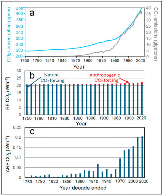
Figure 1.
Atmospheric carbon dioxide CO2 concentration (part (a), blue curve) and consequent radiative forcing (RF) by atmospheric CO2 (parts (b,c)) from the beginning of the Industrial Age in 1750 to 2020. Part (a) shows anthropogenic carbon emissions (grey curve) and consequent concentration of CO2 in the atmosphere (blue curve). Part (b) shows the resulting radiative forcing (RF) by atmospheric carbon dioxide (CO2) (RFCO2) at the top of the atmosphere (TOA) calculated using the atmospheric absorption/transmittance code MODTRAN (see Supplementary Materials, or SM). In part (b), red bars show the anthropogenic contribution to RFCO2 while blue bars show the natural contribution. Part (c) is a difference curve of the data graphed in part (b) showing decadal changes in RFCO2, or ΔRFCO2. Part (a) is from the National Oceanic and Atmospheric Administration (NOAA), adapted from the original by Dr. Howard Diamond. Atmospheric CO2 data are from NOAA and ETHZ. CO2 emissions data are from Our World in Data and the Global Carbon Project and were downloaded from https://www.climate.gov/news-features/understanding-climate/climate-change-atmospheric-carbon-dioxide (accessed on 29 September 2025).
Figure 1a shows atmospheric carbon dioxide concentration from the start of the Industrial Age in 1750 until the year 2020 of the Current Era (CE). In 1750 atmospheric CO2 levels were not yet affected appreciably by human activities (but see [6]). The prevailing natural concentration of CO2 in Earth’s atmosphere in 1750 is estimated by the U.S. National Oceanic and Atmospheric Administration (NOAA) as 277.75 parts per million by volume (ppmv) (Figure 1a; Table S1 in the SM), which is within the typical range observed at the end of recurrent Great Ice Ages (180–300 ppmv). The corresponding RFCO2 in 1750, calculated at the top of the atmosphere using MODTRAN, is 20.7478 Wm−2 (SM, Part 1), all of which originated from natural (non-anthropogenic) atmospheric CO2. By 2020, atmospheric CO2 concentration had risen to 416.5 ppmv owing to human-sourced emissions and the corresponding RFCO2 returned by MODTRAN is 22.1364 Wm−2 (SM, part 1).
Because the increase in atmospheric CO2 since 1750 is attributed to human activities [20,22], the human contribution to CO2 forcing during the Industrial Age is the difference between CO2 forcing in 1750 and 2020, or 1.3886 Wm−2 (22.1364–20.7478 Wm−2) (Figure 1b). The anthropogenic contribution to all CO2-forced planetary warming from the start of the Industrial Age to 2020 is therefore 6.27% of the total forcing induced by atmospheric CO2 in 2020 ([1.3886 Wm−2/22.1364 Wm−2] × 100). All remaining CO2 forcing since 1750, i.e., 93.73% of total CO2 forcing, is natural in origin (Figure 1b). The conclusion cited above from the IPCC’s Fifth Assessment Report that well-mixed greenhouse gases have “unequivocally” enhanced the greenhouse effect “substantially” is not supported by these empirical data, at least for the case of atmospheric CO2.
The physical mechanism underlying the negligible increment in anthropogenic CO2 forcing from 1750 to 2020 (Figure 1) is the well-documented diminishing returns in CO2 forcing power as its concentration in the atmosphere increases. Owing to the logarithmic CO2 forcing curve, higher concentrations of atmospheric CO2 cause exponentially smaller increments in radiative forcing (marginal forcing) of temperature ([52], Figure 8b). As a result of today’s higher concentrations of CO2 in the atmosphere, the radiative forcing power of CO2 has dropped to less than one-third of the forcing power in 1750 [52]. Such diminishing returns explain the relatively small incremental effect of anthropogenic CO2 emissions since 1750 on the radiative forcing of global temperature from atmospheric CO2 as its concentration increases (Figure 1b).
The difference time series for RFCO2 (Figure 1c), ΔRFCO2, shows periodicity in which changes in CO2 forcing fluctuate cyclically over time with apparent peaks in 1790, 1860, 1940 and the present. These peaks are congruent with peaks in AAO activity (cf. with Figure 16 below in this paper), which is proposed here to serve as pacemaker of global climate on centennial and millennial timescales. This result is interpreted as temperature forcing of atmospheric CO2 concentration in phase with the AAO, driven by peaks of global warming that vent CO2 from sea to air. This hypothesis is further evaluated in the remainder of this review.
2.2. Carbon Dioxide Forcing over Geologic Time
Changes in atmospheric CO2 concentration therefore played a relatively small role in forcing global climate over the 275-year span of the Industrial Age. A similar conclusion has been reported for most of the geologically-recorded climate record, the Phanerozoic Eon, from ~540 million years (My) ago to the present. Observational evidence is now available on atmospheric CO2 concentration 53 and global temperature 54 across the Phanerozoic Eon in proxy databases based on the combined research of thousands of investigators. These empirical proxy databases enable new quantitative insights into the relationship between atmospheric CO2 concentration and global temperature as far back in time as CO2 proxy measurements are available, approximately 425 My. Data resolution over this period is sufficient to evaluate the CO2/temperature relationship confidently (alpha level or probability, p < 0.05) on My timescales and in time windows that bracket every known period of rapid climate transition during the Phanerozoic Eon, as identified independently by stratigraphy.
Time series based on these paleoclimate proxy databases reveal little visible relationship between atmospheric CO2 concentration and global temperature (T) over the last 425 My (Figure 2), the oldest date for which CO2 concentration is available in the Royer CO2 database [53].
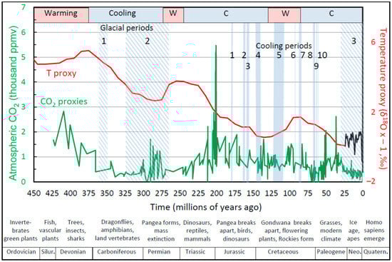
Figure 2.
Time series of proxies of global temperature (red curve) and atmospheric carbon dioxide (CO2) concentration (green curve) over the Phanerozoic Eon [52] (Figure 5). Glacial and cooling periods identified by stratigraphy are labeled with numbers and identified by name in the original figure caption. Evolutionary milestones and geologic periods are shown across the bottom. Averaging of 18O temperature proxy data was done by computing 18O means across windows of 50 My advanced in time increments of 10 My (10–50 running average). This procedure excludes initial values less than half the width of the averaging window, or 25 My, requiring substitution of one-My averaged means in this period for the recent Phanerozoic (black portion of the temperature proxy curve from 25–0 Mybp). Abbreviations: Silur., Silurian; Neo., Neogene; Quatern., Quaternary.
Over some time periods CO2 and T decline together, as in the oldest and most sparsely sampled interval of the Phanerozoic from 425 to 325 My ago. Over other periods CO2 concentration and T increase together, as during the 30 My period from 110 to 80 My ago. Usually, however, CO2 concentration and T appear inversely related. For example, during the longest cold spell of the Phanerozoic Eon, the 50-My Permo-Carboniferous glacial period from ~325 to 275 My ago, atmospheric CO2 concentration more than tripled. Atmospheric CO2 concentration spiked again near the end of the Triassic period ~200 My ago, while global temperature over the corresponding ~50-My time period declined. Atmospheric CO2 peaked during the early and mid-Cretaceous ~125–150 My ago, while global temperature fell to a multi-million year low. The time series panels suggest, if anything, an inverse relationship (negative correlation) between global temperature and atmospheric CO2 concentration.
This hypothesis is confirmed in the scatterplot of atmospheric CO2 concentration versus (vs.) global temperature over the last 425 My (Figure 3). The computed Pearson correlation coefficient (r) between the corresponding proxies is weakly but discernibly negative (r = −0.19, p = 0.006; [52]). The T/CO2 correlation across all known climate transitions during the Phanerozoic is generally (80% of computed correlation coefficients) indiscernible from zero while the rest are almost evenly divided between weakly positive and weakly negative correlations [52].
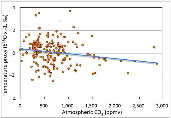
Figure 3.
Scatterplot of proxies of global temperature versus (vs.) proxies of atmospheric carbon dioxide (CO2) concentration (parts per million by volume, or ppmv) across the Phanerozoic Eon derived from oxygen isotope ratios in ancient seashells. The Pearson correlation coefficient (r) is weakly negative (r = −0.19) and discernible at probability (p) = 0.006, i.e., only 3.61% of variance in temperature is explained by variance in atmospheric CO2 concentration (coefficient of determination, or r2, ×100). From Figure 6 in [52].
Although correlation does not imply causation, causation implies correlation, from which it follows that the absence of correlation implies the absence of causation [55,56]. There are exceptions to this general rule under limited and unique circumstances [57,58,59,60], but these circumstances do not apply in the present case. On My timescales, at least, change in atmospheric CO2 concentration was not the cause of global climate change over the last 425 My, a timespan that represents the most recent 78.7% of the geologic climate record.
A prominent recent paper draws the opposite conclusion, suggesting that atmospheric CO2 and global temperature were positively correlated over the last 485 My [61]. On the basis of this correlation, the authors assign causality of natural variation in atmospheric CO2, “as the dominant control on variations in Phanerozoic global climate and suggesting an apparent Earth system sensitivity [Equilibrium Climate Sensitivity or ECS] of ~8 °C.” [61] (p. 1). These conclusions are compromised by five considerations.
- Correlation between CO2 and temperature does not imply causality, as this study asserts without considering criteria for causality (Section 5).
- This study’s conclusion that CO2 is causal to change in T rests on complex, uncertain and unconventional “hybrid” computer modeling of global temperature, with no cross-validation against extensive available empirical databases [62,63,64,65,66,67].
- The temperature time series presented in this study bears little resemblance to empirical proxy data published by hundreds of investigators (cf. Figure 4a in [61] with Figure 3 in [52]), which is reproduced above as Figure 2. Their modeled temperature reconstruction shows no sign of the well-established gradual and steady cooling of the Earth over the Phanerozoic Eon, and no evidence of the spectral periodicity of Phanerozoic temperature time series (Figure 2) that has been reported by numerous investigators as ~120–135 My [52,62,63,64,65,66,67].
- This study’s estimate of climate sensitivity of 8 °C is implausibly extreme, the second-highest in the published climate literature (Table 1 in [68] (p. 2)), more than an order of magnitude larger than the smallest available estimates of ECS, 0.52–0.58 °C [69] to 0.9 °C [69,70,71], and up to five times higher than the IPCC estimate (1.5–4.5 °C) [19].
- Despite its conclusion that atmospheric CO2 concentration and global temperature were correlated over the Phanerozoic, this study reports the absence of statistically discernible correlation over the 186-My Mesozoic Era comprising 38% of their study period. This absence of correlation implies the absence of causality, contradicting the paper’s central conclusion, but is dismissed without explanation as the “Mesozoic conundrum” [61] (p. 5).
The empirical demonstration that CO2 and global temperature are generally uncorrelated over the Phanerozoic Eon [52] is based on observational proxy data consisting of O2 isotope ratios in fossil seashells. In contrast, stable isotope temperature proxies recorded in ice-cores over the last hundreds of millennia are strongly and positively correlated with proxies of atmospheric CO2 [72]. Similar strong positive CO2/temperature correlation also characterizes the most recent instrumental temperature record, as reviewed here (Section 6).
This apparent paradox is explained in part by the timing of atmospheric CO2 and temperature changes. If changes in CO2 (ΔCO2) concentration caused the warming that accompanies glacial terminations, then ΔCO2 would precede change in temperature (ΔT), since cause precedes effect. Instead, several independent studies of paleo temperature and CO2 databases conclude that during glacial terminations, ΔT occurs before or simultaneously with ΔCO2 [73,74,75,76], but see [77]. ΔT is reported to lead ΔCO2 for the entirety of the 540 My Phanerozoic Eon [78]. A comprehensive study of eight contemporary instrumental databases finds that in six of the eight cases, ΔT leads ΔCO2 [79]. The time lag (latency) from ΔT to ΔCO2 measured from contemporary observational data is 9–10 months [79], confirmed below in this review, constraining temporally the dynamics of related carbon-cycle feedback that is presumed to operate during climate (temperature) change [52].
The temporal lag from ΔT to ΔCO2 is consistent with and presumably a consequence of the lower solubility of CO2 in warmer water [80]. Because CO2 is less soluble in warmer water, dissolved CO2 is vented together with heat from a warming Southern Ocean (SO) during deglaciation and during any prolonged warming period, such as the positive phase of the AAO (see below). Therefore, temperature increase precedes and then accompanies further increases in atmospheric CO2 concentration.
The increase in atmospheric CO2 concentration during warming is postulated to provide weak feedback amplification of temperature, but the magnitude of this amplification declines exponentially with higher CO2 concentration ([52], Figure 8b) and is a hundred times smaller than the feedback effects of the much more potent greenhouse gas, water vapor [81]. Similar wind-induced increases in heat and atmospheric CO2 have been reported for the Last Glacial Termination (LGT) [82] and for centennial-scale climate change in the Antarctic [83]. Global temperature and atmospheric CO2 concentration are therefore strongly correlated in both ice core and instrumental records not because increased CO2 caused increased temperature, but because the converse—warming sea water causes increased venting of CO2 to raise its concentration in the atmosphere.
2.3. Carbon Dioxide Compared with Other Forcing Agents
The relative significance of radiative forcing by CO2 in affecting global temperature can be appreciated by comparing it with other influences on climate, such as the negative forcing (cooling) induced by airborne particles (aerosols). The forcing attributable to atmospheric CO2 is so small relative to the Earth’s energy budget that 80% of heat captured by CO2 is reflected back into space by aerosols (SM, Part 2).
Independently, satellite measurements of the Earth’s energy budget document empirically the small role of atmospheric CO2. The Clouds and the Earth’s Radiant Energy System (CERES) satellite-based program launched in December of 1999 consists of five orbiting satellites that continuously record both incoming solar radiation absorbed at the top of the atmosphere (TOA) and outgoing thermal (long-wave) radiation returned to space. The difference between absorbed shortwave radiation and reflected longwave radiation is a measure of Earth’s energy balance, with positive and negative values signifying increased and decreased planetary warming and Earth Energy Imbalance (EEI), while zero difference signifies that the Earth’s energy budget is in balance and global temperature remains unchanged [84,85].
Empirical data from the CERES satellite program and in situ measurements during the warming that occurred from 2005 to 2020 disclose a weak positive imbalance between incoming short-wave solar insolation and outgoing long-wave thermal radiation [86], indicating moderate positive forcing and consequent global warming during this 15-year period. This observed EEI is attributed not to the observed increase in atmospheric CO2 concentration, however, but to decreased albedo from clouds and sea ice [86]. A similar conclusion is reported in an independent analysis of CERES satellite data on cloud cover [87]. The change in EEI from all sources during the warming period from 1990 to 2020 has been attributed to variance in negative forcing from anthropogenic aerosol [86,88]. Any weak additional forcing signal from anthropogenic CO2 is lost in the EEI noise.
A recent paper on the Earth’s energy budget evaluated using CERES satellite data provides a quantitative estimate of the role of atmospheric CO2 in forcing global temperature [89]. The contribution from CO2 is reported as 27% of the total EEI (SM, Part 3), similar to the 20% reported by Taylor [51], [90] (p. 221), and the maximum 22% inferred by Nikolov and Zeller ([87], Figure 7). Similarly, Scafetta estimates that “at least 60% of the global warming observed since 1970 has been induced by the combined effect of natural climate oscillations,” leaving at most 40% for all other sources, including all greenhouse gases and CO2 [91] (p. 1). Since an estimated 76% of forcing from greenhouse gases is from CO2 [19], this leaves at most 30.4% for CO2.
These are among the best available quantitative estimates of the forcing contribution of anthropogenic CO2 based on empirical data as opposed to computer models. Averaging all of these sources, a mean estimate of the contribution of atmospheric CO2 to climate forcing in this century is ~25%, with a relatively large error variance that however never exceeds 50% total CO2 contribution, i.e., under no circumstances is atmospheric CO2 a majority contributor to climate forcing.
These contributions of CO2 to temperature forcing must be evaluated against the above demonstration that 6.27% of RFCO2 between 1750 and 2020 is attributable to anthropogenic CO2 (Figure 1) while the remaining 93.73% is natural in origin. It follows that even if contemporary global warming were 100% attributable to increases in the atmospheric concentration of CO2 instead of the estimated 25%, 6.27% of this forcing would be attributable to human-sourced emissions of CO2. Using the more refined empirical estimates of CO2 contributions developed above, where approximately one-fourth of total forcing is attributable to atmospheric CO2, the maximum contribution of human-sourced CO2 to contemporary global warming is estimated quantitatively from empirical data as 6.27% (the computed contribution of anthropogenic CO2 forcing from 1750 to 2020, above) of 25% (the approximate mean empirical estimate of CO2 forcing of temperature, above), or 1.57% of total temperature forcing.
The remaining 98.43% of climate forcing arises from sources other than anthropogenic CO2. These other sources include all remaining greenhouse gases, particularly water vapor and methane, as well all sources of natural climate variability, including especially natural climate cycles on Earth and variance in total solar irradiance. If the concentration of CO2 in Earth’s atmosphere continues to increase exponentially as it has since contemporary measurements began 67 years ago (see below), then the incremental contribution of CO2 forcing to global warming will continue to decline exponentially because the forcing power of CO2 wanes with higher CO2 concentrations owing to the aforementioned diminishing returns in marginal forcing [52]. These empirical data collectively support the hypothesis that atmospheric CO2 plays a minor and diminishing role in forcing contemporary global warming.
In contrast to these conclusions, a recent paper uses the same methodology as the IPCC, including extensive modeling, to conclude that “for the 2014–2023 decade average, observed warming was 1.19 [1.06 to 1.30] °C, of which 1.19 [1.0 to 1.4] °C was human-induced.” [92] (p. 2625). According to these authors, therefore, all global warming recorded instrumentally in the decade ending in 2023 arose from human-sourced CO2 emissions. This conclusion is not consistent with the observation that global temperature has increased by 1.1 °C not in the most recent decade of this century, but since 1750 [93]. As documented above, several empirical studies suggest that increased forcing in this century is not primarily attributable to atmospheric CO2 (op. cit.); see further [86,87,88,89,91,94] and below. The second conclusion of this paper [92], that anthropogenic CO2 emissions are abating, is likewise inconsistent with empirical data, in this case the Keeling Curve (see below). This universally accepted time series shows an ongoing exponential increase in the concentration of CO2 in the atmosphere and its rate of increase since recordings began in 1958.
The conclusion that atmospheric CO2 plays a secondary role in modulating global climate is consistent with the finding that isotopic signatures of atmospheric CO2 since the Little Ice Age show a weak contribution of anthropogenic CO2 [95,96,97,98,99,100]. The total CO2 flux to the atmosphere from human activities since the onset of industrial age as evidenced by isotopic signature has been estimated as 4% [20,22,98]. These observations raise the possibility that CO2 emitted to the atmosphere by human activities may represent a smaller fraction of the total atmospheric CO2 load than usually accepted, although this conclusion is debated [100].
Widely-accepted empirical data from diverse, independent sources therefore collectively suggest that radiative forcing of temperature by atmospheric CO2 is substantially smaller than theoretical estimates derived from computer models [91,101,102,103,104,105]. The well-documented GE of atmospheric CO2 assures at least modest contribution to climate change from human-sourced emissions, but this impact is estimated quantitatively here using standard and widely accepted data and methods as a small fraction (1.57%) of the total forcing induced by atmospheric CO2. Such forcing is typically computed at the TOA, however, and is smaller at the Earth’s surface. The only available direct surface measurement of increased forcing by CO2 as detected by atmospheric emitted radiance interferometer spectra over two recent decades returned a value of 0.2 Wm−2 per decade as the increase in forcing at the Earth’s surface attributable to changes in atmospheric CO2 concentration [49].
This single empirical measurement of CO2 forcing at the Earth’s surface, equivalent to an increase of 0.02 Wm−2yr−1, compares with 1061 Wm−2 of solar insolation at the TOA (the solar constant; [106]) and 1001.4 Wm−2 at the Earth’s surface (“1 Sun”) under specific, idealized measurement conditions [107]. After compensating for the near-spherical geometry of the Earth and the day-night cycle, averaged incoming solar energy across the entirety of the Earth’s surface is estimated as 342 Wm−2 ([108], Table 1, p. 199). Increased annual surface forcing from atmospheric CO2, 0.02 Wm−2 year−1 [49], is therefore a negligible fraction (0.00585%) of the average global surface insolation energy provided by the primary driver of climate, the Sun.
Such a marginal effect of CO2 on temperature is consistent with its small contribution by volume to Earth’s atmosphere (0.04%). Exponentially diminishing returns in marginal forcing based on the logarithmic CO2 radiative forcing curve have already reduced the warming power of CO2 by more than two-thirds since 1750 because increases in CO2 concentration have an exponentially smaller marginal effect on temperature as atmospheric CO2 concentration increases ([52], Figure 8). It seems energetically implausible that a minor trace gas constituting a small fraction of the atmosphere, exhibiting small and diminishing radiative forcing power and comprising a miniscule fraction of a percent of natural climate forcing by the Sun, could generate the enormous energy flux required to account for the mean contemporary global warming signal of 1.1 °C over the Industrial Age [93]. The corresponding calculated heat flux is reportedly equivalent to indefinite, around-the-clock detonation of five Hiroshima-sized atomic bombs per second [109].
These are among the reasons that “… climate models predict too much warming from increased atmospheric carbon dioxide.” [110] (p. 1), [111]. A recent comparison of all climate models concludes that “most models … overestimate recent warming trends … with differences that cannot be explained by internal variability. This probably leads to future warming projections [based on models] being biased high.” [112] (p. 6). A recent weighted comparison of all climate models, including the sixth Coupled Model Intercomparison Project, concluded that “Our results show a reduction in projected mean warming [from CO2].” [113] (p. 1).
Computer models of climate have a more fundamental limitation. They cannot account for, explain, or replicate the natural temperature oscillations [114] that are the most basic and universal property of global climate on all timescales [115], as developed in the next section.
3. Natural Climate Variability
A variety of natural forces are known to influence climate, including chronic, episodic, and periodic. Chronic influences include long-term crustal and mantle cooling and changes in total solar irradiance. Episodic events include volcanoes, dust storms, coronal mass ejections from the Sun, and variation in ocean currents like the Atlantic Meridional Overturning Circulation (AMOC). Periodic events known to affect climate include the 11-year sunspot cycle, longer solar cycles, and geological cycles like plate tectonics and mantle flow patterns. This review focuses on temperature fluctuations induced by identified natural climate cycles that oscillate at periods most relevant to human and civilizational timescales, centennial to millennial.
3.1. Natural Climate Cycles
Natural climate cycles are regional or global temperature oscillations of characteristic repetition frequencies that are driven by non-human forces. Several such cycles have been identified and studied in depth. The repetition period of these natural climate cycles ranges over ten orders of magnitude, from a high of 135–150 My for global temperature over the Phanerozoic Eon [52,62,63,64,65,66,67,115,116] to a low of 40–50 days for the Madden-Julian oscillation [117,118,119,120,121,122].
Between these extremes lie a plethora of well-documented climate oscillations ranging in repetition period from 80 to 120 thousand years (Ky) for the astronomically-driven Great Ice Ages [123,124,125,126] to 30–70 years for the Pacific Decadal Oscillation or PDO, also termed the Interdecadal Pacific Oscillation or IPO [127,128,129,130]; 60–90 years for the Atlantic Multidecadal Oscillation or AMO [131,132,133,134,135,136,137,138,139]; 60–80 years for the Arctic Oscillation, or AO [140,141,142]; 60–90 years for the AAO [39,115,143,144,145,146,147,148]; 3–7 years for the El Niño Southern Oscillation (ENSO) [149,150,151,152]; and 20–36 months for the equatorial Quasi-biennial Oscillation (QO) [153,154,155,156,157,158].
As illustrated by these numerous examples, global climate is fundamentally an oscillatory system. Until computer models of the climate can replicate, explain and accurately hindcast and forecast these well-documented climate oscillations, such models cannot be considered “mature.” Scientific models characterized as “immature” are those that are not sufficiently developed to accurately replicate the natural phenomena they seek to represent and are therefore by definition incomplete, implying in the case of climate models omission of the most basic underlying causal dynamics. The term “immature” in this context is not pejorative, as all scientific models must pass through such early developmental stages. Such immature scientific models do not, however, provide a valid basis for forecasting future climate and making critical and costly policy decisions about climate change. Improving climate models until they can account for and replicate climate oscillations on all timescales is proposed as a priority goal of future climate research (Section 11).
3.2. The Antarctic Oscillation as Global Climate Pacemaker
Exclusion of atmospheric CO2 as the primary cause of global warming invites consideration of alternative hypotheses. Recent empirical evidence supports the hypothesis that global warming and cooling are driven on a centennial timescale by a powerful cycle of atmospheric pressure/wind/temperature (PWT) in the Southern Hemisphere (SH). This centennial cycle is in turn modulated on a millennial timescale (Figure 4) to generate longer warming and cooling cycles. We named this centennial paleo-wind cycle the Antarctic Centennial Wind Oscillation (ACWO) [39,115,145]. The paleo-temperature cycle it drives, the Antarctic Centennial Oscillation (ACO), is the paleohistoric precursor of the contemporary AAO [115,145]. We therefore describe this natural Antarctic temperature cycle by conjoining the two acronyms, i.e., the ACO/AAO cycle or, for brevity and historical currency, the AAO.
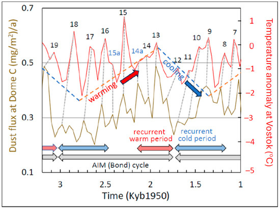
Figure 4.
Wind proxy (dust flux; brown curve) and corresponding temperature proxy anomaly (red curve) in Antarctica during the late Holocene. Gray arrows at the bottom depict the millennial Antarctic Isotope Maxima (AIM) cycle in the Southern Hemisphere (SH), which drives the Bond Cycle in the Northern Hemisphere (NH) (see text). Numeric labels identify cycle numbers of the Antarctic Centennial Oscillation/Antarctic Oscillation (ACO/AAO) temperature cycle, or the AAO. Grey dashed lines connect wind velocity peaks with temperature peaks. Colored bidirectional arrows designate Recurrent Warm Periods (RWPs, red) and Recurrent Cold Periods (RCPs, blue) that correspond most recently to the Medieval Warm Period (MWP) and Little Ice Age (LIA), respectively. The red and blue dashed lines show the approximate average warming and cooling trends, respectively, at Vostok, Antarctica, over the millennium, caused by temporal summation and facilitation of wind cycles (see text). Wind proxies (dust flux) are measured from ice cores at the European Project for Ice Coring in Antarctica (EPICA) Dome C drill site in Antarctica, while temperature proxies are from the nearby Vostok drill site. Modified from [39]. Additional abbreviations: KYb1950, thousand years before 1950; a, annum.
Wind and temperature profiles of the AAO as estimated from proxies retrieved from ice cores extracted from drill sites in Antarctica are shown in Figure 4. Every major centennial wind cycle is followed after a variable delay measured in decades by a corresponding AAO temperature peak here and at ten other major Antarctic drill sites [115]. These centennial wind and temperature cycles are modulated on the same millennial cycle as the ACWO. This thousand-year cycle is identical to that established previously for the Antarctic Isotope Maxima (AIM) cycle and is reflected in the Northern Hemisphere (NH) by the Bond and Heinrich cycles as well as the MWP and LIA (see below).
Numerous studies report the powerful and pervasive effects of the AAO on climate in the SH and worldwide. In the SH, the AAO has long been recognized as the dominant mode of climate variability [159]. This natural climate cycle drives wind intensity, surface temperature, and precipitation patterns, among other climate variables, throughout the SH [160,161,162,163,164,165,166,167,168,169,170,171,172].
The strong influence of the AAO on climate in the NH is equally pervasive. Increases in surface temperature on the Tibetan Plateau (TP) accompany the positive phase of the AAO, which is teleconnected northward from the SH by atmospheric Rossby wave trains with a current (interstadial, warm climate) propagation time of approximately one month [173]. The AAO is correlated with and inferred to at least partly influence summertime rainfall over north China [174] and East Asia [175], burn areas from wildfires [176], ocean wave power across the planet [177,178], the frequency of typhoons in the North Pacific [179,180] and Atlantic [181] Oceans, the intensity of Pacific typhoons [182], the global distribution of pollutants via air circulation patterns [183], a global increase in extreme rain events over land [184], drought and flood hazards [185], coastal flooding associated with sea level rise [186], and even the sovereign debt crisis of nations [187].
Climate changes in the NH associated with the AAO have been reported in dozens of additional studies over the last two decades [162,188,189,190,191,192,193,194,195,196,197,198,199]. These extensive, diverse and powerful worldwide effects of the AAO constitute overwhelming empirical evidence that this natural PWT cycle strongly influences global climate, including northerly climate cycles such as the North Atlantic Oscillation (NAO) and the AO. A 62-year “sinusoidal” temperature cycle similar in period to the contemporary AAO has been identified by Gervais [200] and supported in 20 previous studies cited in the Introduction to that paper. These findings are consistent with the NGW mechanism advanced here, including the hypothesis that the AAO serves as the primary pacemaker of global climate.
The ACWO wind cycle and the AAO temperature cycle that it drives are visible in the ice core record extending to 226 thousand years (Ky) before 1950 (Kyb1950) (Figure 5) [39]. Earlier cycles are not detectable because the temperature proxy record at Vostok for older time periods was not sampled frequently enough to satisfy the Nyquist-Shannon detection criterion of a minimum of two samples per cycle [201,202,203,204]. The form of the millennial cycle and its embedded centennial cycle is similar across these hundreds of millennia (Figure 5), implying that this cyclic pattern is the stereotypic building block of climate change at least as far back in time as Vostok temperature proxy data can be resolved at centennial timescales, 226 millennia.
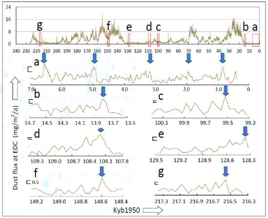
Figure 5.
Proxies of Antarctic wind velocity over the past 226 thousand years (Ky) showing the stereotypic pattern of climate change over recent climate history. The wind (dust flux) record recovered from ice cores at the European Project for Ice Coring in Antarctica (EPICA) Dome C drill site in Antarctica is shown in the top panel. The lower panels (a–g) magnify the time periods enclosed by red rectangles in the top panel. Each lower panel shows a complete millennial cycle of the Antarctic Centennial Wind Oscillation (ACWO) usually containing 6–8 centennial wind cycles that drive the Antarctic Centennial Oscillation (ACO) of temperature, which is the historical precursor of the contemporary Antarctic Oscillation (AAO) temperature oscillation. Blue arrows identify the Wind Terminus (WT) of each ACWO cycle, followed immediately by the onset of the Recurrent Cold Period (RCP). Calibration scales in (a–g) correspond to 0.25 mg/m2/annum, except for part (f), where the scale is doubled as labeled. From ([39], Figure 14). Abbreviations: a, annum; Kyb1950, thousand years before 1950.
The AAO is probably older. The high-resolution ice-core dust deposition data at the European Project for Ice Coring in Antarctica at Dome C (EDC) drill site date even further back in time and show similar centennial and millennial patterns, implying that the ACWO wind cycle and the corresponding ACO/AAO temperature cycles are geologically older. These empirical findings support the hypothesis that the millennial ACWO wind cycle and the resulting centennial AAO temperature cycle are the elemental units of global climate change on centennial and millennial timescales, the most immediately relevant timescales to human and civilizational affairs. Global warming increases during the multidecadal rising (positive) phase of each centennial AAO temperature cycle, followed by global cooling during the following multidecadal falling (negative) phase of the AAO. The duration of the positive (warming) phase of the AAO is not discernibly different from the duration of the negative (cooling) phase, i.e., the AAO temperature cycle is on average symmetrical [39,115,142].
The AAO is currently approaching a multi-centennial peak [143,200,205,206] (see also below), as is the coupled AO [207,208], consistent with the hypothesis that contemporary global warming is driven by natural climate variability, namely the AAO. A recent paper suggests that the two-decade slowdown in the loss of Arctic sea ice is caused by natural ocean cycles [209], congruent with the peaking of the AAO driven by natural climate variability. These discoveries answer the earlier reservation [38] that the AGW hypothesis lacks a convincing alternative by providing a well-documented empirical alternative that is the basis of the NGW hypothesis.
3.2.1. Geography
The strongest wind stress on ocean waters anywhere on Earth occurs in the “roaring fifties,” the high southerly latitudes that encompass the broadest reach of the SO. An estimated 80% of the planet’s wind energy is contained in storm tracks over the SO [210]. These powerful winds, and most winds on Earth, can be tracked online at all altitudes and seasons in near-real time and their velocity measured using the powerful educational and research tool Nullschool [211].
This region of the roughest seas on Earth is the likely location for wind-driven upwelling that both closes the AMOC loop [212] and generates the AAO (Figure 6), as revealed by latency measurements for the teleconnected cycle recorded in ice cores on the Antarctic continent [115]. As detailed below in this section, the moving wave of each identified AAO is first detectable on the Eastern Seaboard of Antarctica at the Law Dome drill site and later at “downstream” drill sites. The velocity of this waveform is then calculated and projected backward to establish the origin of the ACWO in the SO East of the Antarctic continent as shown in Figure 6 ([115], Figure 20). The boundaries of this zone have not been demarcated quantitatively and probably vary seasonally and over longer terms based on climate, meteorological and other conditions. These boundaries are approximated based on areas of highest relative mean contemporary wind stress (pink area in Figure 6).
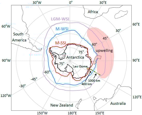
Figure 6.
Approximate site of generation in the Southern Ocean (SO) of the Antarctic Centennial Oscillation (ACO), the paleo-precursor of the contemporary Antarctic Oscillation (AAO). The pink area approximates the area of upwelling driven by westerly winds in the “roaring fifties,” where time-integrated wind stress over open ocean water is higher than any other place on Earth. Upwelling brings heat and carbon dioxide from the depths to the surface during warming, which is attenuated during cooling (see text). The pink arrow symbolizes recruitment of warm upwelling sea water into the Antarctic Circumpolar Current (ACC). Colored lines around Antarctica designate the extent of Antarctic sea ice at different times in climate history. Abbreviations: M, modern; WSI, Winter sea ice; SSI, summer sea ice; LGM, Last Glacial Maximum. From ([115], Figure 20).
3.2.2. Geophysical Mechanisms
A complete understanding of global climate change requires understanding the underlying mechanisms. The availability of plausible mechanisms underlying climate change is also a supporting criterion for establishing causality (Section 5). This section posits the underlying mechanism of climate change on human timescales as a forced relaxation oscillation (the AAO) that is endogenous to the Earth system but ultimately powered by the Sun.
To initiate this oscillation, Westerly Winds blow across the SO to displace cold surface water at right angles to the wind stress (i.e., northward into the tropical Pacific) by Ekman transport or “pumping” and replace it with upwelling warmer, CO2-rich Antarctic Intermediate Water (AAIW) and Sub-Antarctic Mode Water (SAAMW) [213,214,215,216,217]. This broad and powerful regional upwelling releases both heat and CO2 from the SO into the Antarctic atmosphere to cause warming and increased atmospheric CO2 concentration, respectively [213,214,215,216,217,218,219,220,221,222,223,224,225,226,227,228,229,230]. The vented CO2 has minimal marginal impact on temperature owing to diminishing returns in radiative forcing with higher concentration [52] and is mixed rapidly in the atmosphere along with the released heat to spread worldwide within years [231].
As deeper and warmer AAIW and SAAMW are uplifted to the surface of the SO by these Westerlies [216,232,233], they are recruited into the Antarctic Circumpolar Current (ACC) [234,235], the continuous clockwise ocean current that circumscribes Antarctica. During the positive (warming) phase of the AAO, the east coast of the Antarctic continent is exposed first to freshly uplifted warmer water, consistent with the greatest loss of ice and consequently narrowest ice sheet along the Eastern Antarctic seaboard (red line in Figure 6) [236]. The warmer circumpolar water melts the icescape surrounding Antarctica at the base and grounding lines of ice sheets and glaciers [237,238,239,240,241,242,243,244,245,246,247,248,249,250,251] to reconfigure the Antarctic cryosphere and induce progressive deglaciation during each AAO positive (warm) phase.
A second source of warm-water upwelling around Antarctica is driven by cold, descending Dense Shelf Water that sinks nearshore to drive upwelling of warmer waters in offshore return cells [242,252]. Recruitment of this warmer water into the ACC contributes to melting of basal glacial shelves surrounding Antarctica [232,247,253,254,255], including the melting of sea ice on the East Antarctic seaboard [239]. The same geo-mechanisms operate during deglaciations following major ice ages [256].
A third and dominant amplifier of basal ice shelf melting during the positive (warming) phase of the AAO arises from the meridional constriction (poleward compaction) of the ACC [234,257,258,259]. Compaction of the ACC is driven by acceleration of the wind mass that circles above the South Pole, the Antarctic Circumpolar Vortex (ACV), and is required by the laws of physics to reduce rotational inertia and conserve angular momentum, analogous to a spinning ice skater with folded arms. This wind acceleration induces even greater oceanic upwelling in the SO (positive feedback), increases Ekman pumping of cold surface water northward into the equatorial Pacific [260,261,262,263], and brings uplifted warmer water from the periphery of the ACC circulation at the margin of the Polar Front (PF) into contact with ice shelves and glaciers on the edge of the continent [144,215,264,265,266].
At the same time, this meridional poleward constriction of the ACC combines with increased poleward transport of heat from heightened regional eddy activity that transfers heat vertically [82,215,217,218,219,220,221,223,226,227,228,230,240,258,267,268,269,270,271,272,273,274,275,276], as shaped and directed by bottom topography [277]. These forces combine to induce net poleward heat transfer in ACC surface and near-surface waters to create and reinforce the developing positive or warming phase of the AAO [234,239].
In this process of poleward compaction, the difference in Sea Surface Temperature (SST) from the PF to the Antarctic shoreline during the peak positive phase of the ACO/AAO can reach 16 °C [234]. These wind-and temperature-driven oceanic responses transport heat poleward and focus this heat on the Antarctic ice margins to sculpt the Antarctic icescape and teleconnect the ACO around the coastline of Antarctica [218,237,238,241,245,246,247,248,278,279,280,281,282]. The thaw is supplemented by warmer glacial meltwater during the Antarctic summer [283].
As a result of these atmosphere/ocean dynamics in the SO, each peak in ACWO wind intensity is accompanied 1:1 after a short (decadal) and variable delay by a peak in Antarctic temperature (Figure 4). This same climate mechanism explains the relationship between temperature and atmospheric CO2 concentration during glacial terminations. Heat and atmospheric CO2 increase together owing to wind-driven oceanic upwelling and venting of both, with acceleration of CO2 release by warming of sea water and consequent venting of additional CO2 to the atmosphere [77,82].
Each AAO cycle is completed by the negative or cooling phase, which is triggered by the preceding warm phase. As powerful Westerly winds blow across the SO to induce upwelling and cause each warming cycle of the AAO, the SH warms as described above. Warming of the SH reduces the temperature gradient between the equator and the poles. This temperature gradient is the heat engine that propels the ACV, as well as the ACWO wind cycle and its accompanying temperature cycle, the AAO. When the equator-to-pole temperature gradient declines, i.e., when the SH warms, the velocity of the ACWO wind declines. This drop in wind velocity reduces oceanic upwelling, retaining cold surface water at higher polar latitudes, restoring colder temperatures in the Antarctic, and at least partially rebuilding the SH cryosphere. The consequent drop in temperature of the SH comprises the cooling phase of the AAO. As it progresses, the equator-to-pole temperature gradient increases, recharging the heat engine that drives wind velocity in the SH [284,285,286,287]. Restoration of the heat engine caused by cooling in the SH regenerates renewed strong ACWO westerly winds propelled by the ACV to initiate the next positive or warming phase in the ACWO millennial sequence.
The geophysical mechanisms of the AAO summarized above correspond to the well-known process of forced relaxation oscillation, by which each phase of a cyclic process initiates and supports its opposite phase by inbuilt feedbacks with delays. The cycle is endogenous to the Earth system but forced externally by a continual input of solar energy. The concept of relaxation oscillation was developed originally in the field of electronics [280,288,289] and has found numerous applications in other disciplines including climate science [290,291,292,293,294,295,296,297]. In the case of the AAO, global warming triggers global cooling and conversely, cooling triggers warming, with inbuilt delays that are imposed by the properties of the physical system that is oscillating, namely the coupled hydrosphere/atmosphere/cryosphere. In this interpretation of natural climate variability, the ACWO and the AAO temperature cycle that it drives represent the output of a forced relaxation oscillator, with the driving energy supplied by the equator-to-pole temperature differential that is powered ultimately by the Sun [284,285,286,287].
Unanswered questions remain in this presumptive causal sequence. For example, “Direct evidence for the postulated warming from intermediate water records is … lacking, and the processes controlling low-latitude intermediate temperature evolution remain unclear.” [298] (p. 1293). Similarly, “… a variety of mechanisms have been proposed to play a role in AAIW formation, but no agreement has been reached.” [250] (p. 2873). Additionally, “interannual variability of off-shelf zonal winds has a minor effect on ocean heat intrusion into [Pine Island and Thwaites Ice Shelf] cavities, contrary to the widely accepted concept.” [242] (p. 1). These and other evidentiary gaps appear relatively minor and can presumably be filled by further oceanographic research.
3.2.3. Teleconnection
The AAO temperature oscillation is propagated (teleconnected) westward from its site of origin in the SO (Figure 6) to the Antarctic continent and northward to the rest of the globe. The movement of the AAO cycle can be traced to and across Antarctica by measuring the time it takes for the peak of each identified AAO temperature cycle to reach successive drill stations across the continent. The Law Dome drill station is among the first to record the peak of each AAO cycle, as expected from its location on the east Antarctic coastline nearest the site of AAO generation. The arrival time of the AAO at Law Dome is therefore defined as zero latency. The peak of the same, identified AAO cycle can then be detected from centuries to millennia later at ten additional Antarctic drill stations distributed widely across the continent and from sea level to 4000 m at the top of the East Antarctic Plateau (EAP) to trace the path and velocity of the moving AAO waveform.
During the Last Glacial Maximum (LGM), the latency of the moving temperature peaks of AAO warm phases is small (less than 500 years) to downstream coastal drill sites, medium (500–750 years) to somewhat-elevated inland sites, and greatest (750 to more than 1000 years) to the highest drill sites on the EAP (Figure 7a) [115]. The mean velocity of the ACC is ~4 km/hr., implying that this clockwise ocean current circumscribes the ~16,000 km Antarctic shoreline in ~167 days. The teleconnection of the AAO to Antarctic drill stations is therefore orders of magnitude slower than the flow velocity of the ACC, consistent with the thermal inertia of the Antarctic icescape.
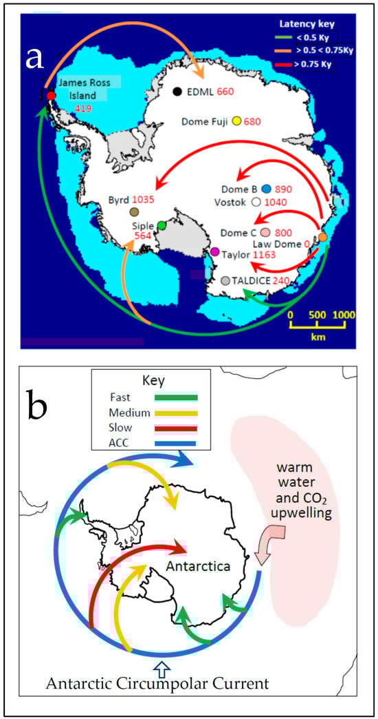
Figure 7.
Teleconnection latencies (a) and consequent propagation velocities (b) of the Antarctic Centennial Oscillation/Antarctic Oscillation (ACO/AAO) during the Last Glacial Maximum (LGM). Red numbers in part (a) represent the latency in years from Law Dome to the indicated drill sites. Teleconnection is fastest along the coastline, where heat is transported by the rapidly-moving waters of the Antarctic Circumpolar Current (ACC), and slowest to the highest elevations on the East Antarctic Plateau (EAP), where heat is transported upslope from marine sites through the atmosphere against katabatic wind flows. Abbreviation: Ky, thousand years; EDML, the European Project for Ice Coring in Antarctica (EPICA) drilling site at Dronning Maud Land (DML), Antarctica. From ([115], Figure 6 (part (a)) and graphical abstract (part (b))).
During the LGM, the fastest teleconnection (lowest latency, green arrows in Figure 7b) is mediated by upwelled heat captured by and transported within the rapidly moving water of the ACC (blue arrow in Figure 7b) as modulated by its interaction with the Antarctic icescape [115]. The intermediate teleconnection latency (orange arrows in Figure 7b) is proposed to result from a mix of marine and atmospheric propagation. The slowest teleconnection latency (red arrows in Figure 7) is inferred to originate from a combination of rapid marine transport of heat to downstream coastal locations carried by the ACC, followed by slower upslope atmospheric transport against the katabatic wind circulation to the highest and coldest elevations on the EAP, ~4000 m above sea level at Vostok and Dome C [115].
In contrast to long propagation latencies in a cold climate, during the warmer Holocene climate that followed the LGT the latency of each AAO peak on its journey from Law Dome on the east coast to downstream drill sites declined by several orders of magnitude, implying that teleconnection velocity is greater in warmer climates. Teleconnection latency to downstream drill sites during the Holocene is measured in years rather than millennia [115] and averages to near zero, i.e., teleconnection of the AAO to and across Antarctica during warm climates is near-instantaneous within likely error limits.
The faster teleconnection is presumably related to the concurrent higher temperature and greater humidity that accompanies warming and a consequent shift from marine teleconnection to faster atmospheric mechanisms of teleconnection. These findings collectively support two modes of teleconnection during cold climates: fast oceanic, and slow atmospheric, opposite from the phenomenology of northward teleconnection of the ACO/AAO (slow oceanic and fast atmospheric transport; see below). In a warmer climate, fast atmospheric transport prevails both in the SH and globally.
In addition to its westward propagation across Antarctica, the AAO simultaneously travels northward from its site of generation in the SO to the rest of the globe. The latency of northward teleconnection of the AAO has been measured empirically as the difference between the time of occurrence of AIMs in the SH to the resulting Dansgaard-Oeschger (D-O) events in the NH. This propagation latency is 2–3 Ky during the cold LGM, but orders of magnitude faster—months to decades—during interstadials such as the Holocene, when global temperatures are several degrees C warmer (op. cit.).
Teleconnection of AAO cycles northward during cold climates follows the same temperature dependence as within the SH. Slower northward teleconnection of the AAO is consistent with slow (millennial) ocean currents that distribute heat globally (i.e., the AMOC), while more rapid northward teleconnection during warmer climates is regulated by faster atmospheric processes, such as Rossby wave trains [173]. This mechanistic phenomenology is reverse from that postulated for the teleconnection of the AAO within the SH, as described above. For the northward propagation of the ACO/AAO to form D-O events in Greenland, the oceanic propagation that predominates during cold, dry glacial periods is slow, requiring millennia to complete the hemispheric transit. In contrast, during warmer and more humid periods of interstadial climates, atmospheric propagation prevails and is orders of magnitude faster.
Several additional and well-known decadal-to-centennial-scale climate cycles characterize the global climate as summarized earlier in this review (Section 3.1). The empirical data summarized here and below are consistent with the hypothesis that the ACWO wind cycle and accompanying AAO temperature cycle are the driving forces behind all of the more northerly climate cycles. Global climate on human and civilizational timescales is conceived as an interacting assemblage of forced climate oscillations linked across the globe by atmospheric and oceanic processes and interactions. We proposed that these cycles are linked and interdependent and coupled with and forced by the most energetic of all such cycles, the AAO [39]. Recent studies confirm this hypothesis for the AAO and the AO, perhaps the two most influential natural climate cycles on Earth, which are coupled by stratospheric meridional wind circulation [208]. This CO hypothesis is developed in greater detail below.
4. A Unified Theory of Climate
4.1. Definition
Albert Einstein coined the phrase “unified theory” in pursuit of a general explanation of all the major forces of particle physics, from gravity and electromagnetism through strong and weak nuclear forces, within a single conceptual framework that could integrate and account seamlessly for all. To generalize this concept to all disciplines, a unified theory explains not a single phenomenon, but rather a host of related phenomena whose interrelationships were not previously understood. Applied to climate, a unified theory would explain not only global warming, but additional milestones of climate change, including global cooling and related climate landmarks such as all natural climate cycles, warm periods such as the MWP and cold periods such as the LIA. A unified theory represents a scientific advance in that it explains previously disparate phenomena and their interrelationships within a single conceptual framework with heightened explanatory and predictive power, which are the ultimate goals of science. This section introduces a unified theory of climate based on the AAO and shows how it is capable of explaining disparate climate phenomena whose origins and interrelationships were not previously understood, beginning with the underlying mechanisms.
4.2. Mechanisms
Two properties of the ACWO are key to understanding the origin of major climate milestones generated by the AAO, temporal summation and temporal facilitation. Temporal summation is a concept borrowed from the neurosciences [299,300,301]. As applied to climate, it describes the observed algebraic addition or “piggybacking” of successive ACWO wind cycles over the thousand-year AIM cycle and a corresponding increase in mean Antarctic and global temperature. Each successive wind cycle adds together with the residual wind velocity elevated by the previous cycle to create a higher wind velocity than would otherwise occur. The result is a several-century period of increasing average wind velocity and therefore increasing mean temperature.
Temporal summation across successive centennial ACWO cycles is explained simply by the repeated onset of each ACWO cycle before the preceding cycle has fully recovered [39]. Temporal summation is manifest across millennial ACWO wind cycles as a rise in mean wind velocity and corresponding temperature across successive cycles (Figure 4, red dashed line, and Figure 5) during the first half of each ACWO wind cycle, followed by a rapid-onset and then prolonged cold period (blue dashed line in Figure 4). These alternating warm and cold periods steadily increase in amplitude over each millennial cycle to create the Recurrent Warm Period (RWP) and then rapidly collapse into the linked Recurrent Cold Period (RCP). These alternating warm and cold eras are each a few centuries in duration and correspond most recently to the MWP and LIA, respectively (see below, Section 4.3.2).
The centennial ACWO wind cycle is characterized also by temporal facilitation. This concept, also borrowed from the neurosciences [302,303,304], describes the observed increase in the absolute amplitude of successive centennial wind cycles across the millennial ACWO wind cycle (Figure 4 and Figure 5). Earlier cycles are therefore smaller in absolute amplitude than later “facilitated” cycles. The AAO temperature cycles that are caused by these wind cycles and accompany them 1:1 show similar characteristics, but are not as well defined at any one Antarctic drill site as the wind cycle that drives them all, possibly owing to regional meteorological differences between Antarctic drill sites.
The mechanism(s) underlying temporal facilitation of ACWO wind cycles has not been determined. We speculated that the increase in amplitude of successive wind cycles results from the progressive conditioning of the Antarctic cryosphere over successive cycles of the ACO/AAO, and the consequent iterative acceleration of teleconnection velocities resulting in larger wind and temperature extremes in successive ACWO cycles [39]. The last cycle of each millennial wind cycle sequence, which we termed the WT, is invariably the largest, and triggers or at least precedes a subsequent several-century RCP, the most recent of which is the LIA (see below). Temporal summation and facilitation of the SAM/AAO are visible in time series published by previous investigators ([143], Figure 2c), ([165], Figure 6).
4.3. Climate Landmarks Explained by the Unified Theory
As reviewed in this section, summation and facilitation within the AAO climate cycle are the proposed causes of centennial climate changes such as periodic global warming and cooling, and millennial climate change, including Antarctic Isotope Maxima (AIMs) and D-O oscillations.
4.3.1. Antarctic Isotope Maxima and Dansgaard-Oeschger Oscillations
ACWO wind cycles summate and facilitate over time to culminate at the end of each millennial AIM cycle in the largest PWT excursion of the cycle, the WT (Figure 4 and Figure 5). These summated and facilitated wind velocity maxima, and the corresponding temperature profiles they induce, correspond to the AIMs identified by previous investigators [142,305,306,307,308,309,310]. Each AIM cycle is matched 1:1 with large (10–16 °C) and fast (decadal) temperature increases recorded in Greenland ice cores as D-O oscillations [306,311].
The time delay between AIM cycles in the Southern Hemisphere and the D-O oscillations that they induce in the NH varies with mean global temperature. During warm interstadials, teleconnection of the AIM cycle from south to north is rapid, from days to weeks [76]. In contrast, the south–north transmission latency is orders of magnitude longer during colder ice ages and glacial maxima, from 2 to 3 millennia [306,308,311].
The discovery that fastest teleconnection characterizes warm periods while slower teleconnection predominates during cold periods implies different modes of south-to-north teleconnection. Rapid teleconnection of the AIM signal to the NH during warm periods may take place through the atmosphere, while slower teleconnection may reflect the global redistribution of heat via slower ocean currents, particularly the AMOC [312]. The same relationship between temperature and teleconnection velocity characterizes the ACO as it propagates westward to the Antarctic continent from its source in the SO east of Antarctica [115], although the proposed underlying propagation media are reversed (Section 3.2.3).
Diverse explanations for D-O events have been offered. Our interpretations concur with previous studies cited above showing that D-O events are northerly expressions of AIM cycles in the SH. D-O oscillations are therefore forced millennial climate cycles in the NH that are driven by natural oscillations of climate in the SH (the AAO) that teleconnect northward. Small temperature excursions in the SH—namely AIM events representing peak temperature anomalies of a few degrees C—exert a disproportionate influence on climate in the NH as D-O temperature excursions that are larger in amplitude, 10–16 °C. This interhemispheric amplification has not been noted previously, and its underlying mechanism is unknown. Direct empirical evidence nonetheless establishes that small temperature excursions in Antarctica drive warming episodes in the Arctic that are an order of magnitude larger than the increase in global temperature since 1850 (~1.1 °C) [313]. This empirical finding is central to the assignment of causality in climate science (Section 5).
4.3.2. The Medieval Warm Period and Little Ice Age
Temporal summation and facilitation of the ACWO wind cycle can explain not only AIMs and D-O oscillations, as described in the preceding section, but also multicentennial climate cycles including the MWP and LIA [39]. During the last half of every millennial AIM cycle, summation and facilitation across sequential ACWO cycles contribute to a several-century period of progressively stronger wind velocity and consequent net mean Antarctic warming (dashed red line in Figure 4). At the end of each millennial AIM cycle, the largest wind peak of the sequence, the WT (Figure 4 and Figure 5), initiates a several-century period of net Antarctic cooling. These alternating, long-term warming and cooling periods in the SH (Figure 4) are teleconnected northward to manifest most recently as the MWP and LIA, respectively.
These landmark global climate events are not singular occurrences or anomalous episodes that occurred only once in climate history. Rather, their unique signatures of recurrent, alternating, several-century warm and coupled cool periods are documented in ice core proxy records of corresponding wind profiles in nearly identical stereotypic form for at least the last 226 millennia (Figure 5). Global RCPs are correlated closely with glaciated cold periods established independently by stratigraphy [314,315] for at least the last three millennia, the only time periods for which the necessary stratigraphic data are available. These findings are consistent with comparable transdisciplinary inferences about recurrent warm and cold periods as drawn from geophysical, archaeological, and historical evidence [316].
The source of the millennial periodicity in the ACWO is unknown. The thousand-year cycle could be endogenous to the Earth system, resulting, for example, from the process of relaxation oscillation in which temporal summation and facilitation of the ACWO wind cycle build to a crescendo and then re-set the ongoing climate oscillator with the WT. In this case the millennial periodicity is established by the physical properties and feedback delays in the interacting air–sea-ice system that is undergoing relaxation oscillation. Alternatively, these millennial events could be exogenous, imposed from outside the Earth system, and driven, for example, by a millennial solar cycle, e.g., the Eddy Cycle or the Gleissberg Cycle [39], or other, unidentified millennial cycles. Further research is required to clarify these and other options.
4.3.3. The Bond Cycle and Heinrich Events
Bond events are periodic ice-rafting episodes in the NH during the Holocene defined by iceberg melting and consequent depositions of the debris frozen within them on the floor of the North Atlantic [317,318,319,320]. The Bond cycle has been correlated with global climate change [321,322,323,324,325,326,327,328] and detected in remote regions of the SH such as the central Andes of South America [329]. The Bond cycle was originally thought to oscillate at a period of 1470 years, but that estimate has been reduced to roughly millennial scale [330], similar to the AIM cycle in the SH. Individual Bond events are correlated with D-O events [318], which as documented above are 1:1 expressions in the NH of AIMs in the SH. This correlation establishes the linkage between the millennial Bond Cycle and the AAO.
The cause(s) of ice rafting events like the Bond cycle have been vigorously debated. Bond and colleagues originally attributed the periodicity to a solar cycle [318,319,320]. Others interpreted Bond events as artifactual or statistical noise [330,331], astronomical influences [332], or the gravitational influence of the moon [333]. Past disagreements about the period and even the existence of Bond events are reconciled here by the demonstration of large variability in the teleconnection time from the SH to the NH as a function of global temperature. Latency from AIMs to D-O events is short (years) during warm interstadials, but long (Ky) during cold stadials, leading to the large variance observed in the periodicity of Bond events in the NH. D-O events extend at least back to the penultimate (Eemian) glacial period from 116 to 130 thousand years ago (Kya) [334], implying that linked Bond events are equally ancient. The close linkage between D-O oscillations and Bond events [318], together with the demonstration that D-O events are caused by AIMs in Antarctica, supports the inference that AIMs in the SH cause Bond events in the NH.
Heinrich events are episodic discharges of icebergs in the NH associated with relative warming spells during the LGM, similar to and overlapping in time with Bond events. Heinrich events, like Bond events, are evidenced by layers of ice-rafted debris in marine sediment of the North Atlantic. Heinrich events have been detected in climate records extending as far back as the Jurassic [335]. At least nine such events have been identified since the deglaciation that ended the LGM if the Younger-Dryas period is included as the first, as proposed by some authors [318,336]. They occurred on average every 8 thousand years [337] (range 4.8–15.0 Ky, σ = 3.2 Ky, calculated from [338]). Independent analysis of smaller numbers of Heinrich events gives mean spacing of 7.0 Ky (sample size or n = 2 [338]) and 9.0 Ky (n = 2 [318]). Heinrich events were therefore cyclic [337], but irregular, i.e., their mean period shows considerable variance. The temperature record associated with each Heinrich event rose rapidly (within years) to a maximum temperature and decayed slowly (over centuries to a millennium or more), reminiscent of the time profile of D-O events but on an expanded scale. Ice rafts associated with five Heinrich events originated from the Laurentide Ice Sheet, while two may have originated more from European ice sheets [338].
Heinrich events were originally thought to trigger major worldwide climate events [336,338]. Subsequent research suggests the converse, i.e., Heinrich events are the effects of global climate change elsewhere [339], including Antarctica [340]. Modeling studies implicate linkages with some but not all D-O events [341], but the linkage is compromised by the uncertainties associated with different timescales of bottom sediment and corresponding temperature changes. The long period between Heinrich events suggests a slower underlying process such as perturbations in the AMOC [222], with slowdowns leading to warm-water accumulation at the surface and consequent destabilization of ice sheets [342]. Given that Heinrich events occur during the coldest phase of the Bond Cycle, it is also possible that Heinrich events are Bond events that are amplified by an expanded and therefore destabilized ice pack, though this hypothesis has apparently not been explored. Many authors have noted connections between the Bond Cycle and Heinrich events, but further research is required to clarify possible linkages. Confirmation of this identity would simultaneously help establish the relationship between Heinrich ice-rafting events and the AAO (AIMs) in Antarctica.
4.3.4. The Rise and Fall of Human Civilizations
The impact of climate change on human evolution and affairs is widely appreciated. The identification of the natural cycle that may drive climate on human and civilizational timescales illuminates with new precision the possible depth and breadth of this impact. The temperature cycle driven by the ACWO and the RCPs and RWPs that it induces on multicentennial timescales appear to have shaped human civilizations for as long as they have existed. Every major known civilization of the past four millennia has risen and flourished during RWPs such as the most recent MWP and declined and collapsed near or during RCPs such as the most recent LIA (Figure 8) [39]. These empirical data suggest that the AAO has served as the chief natural pacemaker of the rise and fall of human civilizations. Numerous other forces contribute to such civilizational declines—invasions, wars, revolutions, famine, disease, exhaustion of resources, environmental pollution, politics, ideology, etc.—but the evidence reviewed here suggests that these are secondary and derivative effects. The proximate cause of the major civilizational cycles may be climate change driven by the AAO, with these derivative effects adding to and amplifying the civilizational cycle.
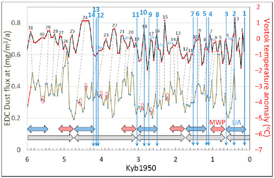
Figure 8.
The rise and fall of the fourteen largest human civilizations of the past four millennia (termination dates indicated by vertical blue arrows) has coincided closely with Recurrent Cold Periods (RCPs), of which the Little Ice Age (LIA) is the most recent example ([39], Figure 7). The identity of the civilizations represented by labels across the top of this figure and by the corresponding blue vertical arrows is provided in the caption to ([39], Figure 7). Additional abbreviations: MWP, Medieval Warm Period; EDC, EPICA Dome C; EPICA, European Project for Ice Coring in Antarctica; Kyb1950, thousand years before the year 1950. The generally accepted dates of civilizational terminations are drawn from historical data assembled in [343] and supplemented by additional sources [344,345,346,347,348,349,350]. Numerals and accompanying letters on the temperature-proxy time series label identified AAO cycles, while red circles on the wind-proxy time series identify peaks that are not clearly associated with a temperature peak. See text for derivation of long-term cycles portrayed beneath the time series.
The congruence of prolonged Recurrent Cold Periods (RCPs) with civilizational decline is not surprising given that each of these past human civilizations was supported by extensive, sophisticated and productive agricultural systems. The freezing weather, drier atmosphere, drought and shortened growing seasons that accompany RCPs such as the most recent LIA make it harder to grow enough food to support large human populations, and as a result the corresponding civilizations decline, disintegrate and disburse. The human population then reorganizes itself into new civilizations with the onset of the next RWP, which supports renewed bountiful agricultural production. In this interpretation the rise and fall of human civilizations is also a forced oscillation coupled with Earth’s climate system, and, in particular, with the AAO and ultimately driven by the Sun.
5. Criteria for Causality in Science
Defining causality is essential for the attribution of the effects of climate change, but this goal has long vexed scientists, historians, legal scholars and philosophers. The modern scientific “gold standard” of causality, the randomized, double-blind, controlled experiment, is usually confined to the laboratory and unavailable to climate science, which is based mainly on observation and modeling of natural phenomena. Climate scientists have written extensively about the causes of climate change even though criteria for causality have not been broadly defined, discussed, or accepted by consensus. This definition void has led to uncertainty, ambiguity and contradiction in the attribution of causality in climate change.
To illustrate, according to older IPCC recommendations [17], causality in climate science requires: (1) “the … detected change [the effect] is consistent with the estimated responses to the given combination of anthropogenic and natural forcing,” and (2), the detected change is “not consistent with alternative, physically plausible explanations of recent climate change.” These IPCC criteria have been cited as the basis of conclusions such as “our study unambiguously shows one-way causality between the total Greenhouse Gases and GMTA [Global Mean Temperature Anomaly]” [351].
The above IPCC criteria for causality on which this attribution is based are inadequate, however, for several reasons. The first IPCC criterion incorrectly assumes foreknowledge of the studied events, introducing several forms of potential outcome bias and logical circularity. The second IPCC criterion likewise incorrectly requires prejudgment of “plausibility” when such criteria cannot be known in advance, again biasing outcomes and inducing circularity. Perhaps most telling, the phrase “consistent with” in IPCC criterion (1) above can imply correlation, not causation, and the two are not equivalent. Likewise, the phrase “not consistent with” in IPCC criterion (2) above may imply that the absence of evidence may be construed as evidence of absence, which is also false.
In any field of science, precise and explicit criteria for causality are required to weigh competing hypotheses objectively on the same scientific scale. We suggested [39] that in climate science, and extending potentially to other scientific disciplines, the contrafactual framework of causality introduced by the 18th century philosopher David Hume [352] and elaborated for modern usage by the late David Lewis [353,354,355], among others, is a useful starting point for this discussion.
5.1. Temporal Order of Cause and Effect
Temporal order is central to causality in Hume’s formulation and to any commonsense definition of causality. That is, a cause-and-effect relationship requires that event c (the cause) precedes in time event e (the effect). This condition of causality may be described as the “temporal order, “or “temporal precedence,” or simply the “temporal criterion.” The delay between cause and effect may be vanishingly small, as the acceleration of a body caused by the application to it of force, but it is still finite and obligate for the demonstration of causality.
5.2. Necessity and Sufficiency
The counterfactual framework rests on the proposition that causation can be defined in terms of “counterfactual conditionals,”, i.e., “If event c [the cause] had not occurred, event e [the effect] would not have occurred.” [352] In this formulation, event e is caused by event c if and only if (iff) event e would not have occurred unless event c occurred. Lewis [353] elaborated on the contrafactual framework of causality as follows:
“Where c and e are two distinct possible events, e causally depends on c if and only if, if c were to occur e would occur; and if c were not to occur e would not occur.”[354], cited from [352]
The two conditions implicit in the above quotation reduce to “sufficiency” (first clause) and “necessity” (second clause). “Sufficiency” means that the occurrence of event c is partially or wholly adequate (sufficient) to the occurrence of event e, while “necessity” means that event c must occur in whole or part (is necessary) in order for event e to occur.
5.3. Applying Causality Criteria to Climate Change
Causality in Hume’s formulation is therefore defined by three “canonical” criteria: temporal precedence, necessity, and sufficiency. Applying these three criteria for causality to climate change, increasing atmospheric CO2 concentration (event c) is causal to global warming (event e) iff c precedes e in time (the temporal criterion), and iff changes in atmospheric CO2 concentration are both necessary and sufficient to changes in global temperature (the counterfactual criteria). As reviewed above (Section 2.2), atmospheric CO2 and global temperature are typically uncorrelated on My timescales over the last 425 million years [52], during which time the mean global temperature dropped by 8–9 °C. Therefore, independent of the temporal criterion, ΔCO2 is not necessary to ΔT.
Similarly, ΔCO2 is not accompanied by ΔT across the full recorded natural history of the CO2/T relationship (e.g., Figure 2 and Figure 3). Strong CO2/T correlations characterize ice core records from the last millennium, but in such records ΔT precedes ΔCO2, violating the temporal criterion for the hypothesis that change in CO2 causes change in T. It follows that changes in atmospheric CO2 concentration are not sufficient to changes in global temperature. Therefore, changes in atmospheric CO2 concentration are neither necessary nor sufficient to induce climate (temperature) change, and consequently, CO2 was not the cause of climate change across the last 425 My, irrespective of any additional criteria for causality that may be applied (see below in this section).
The criteria of necessity and sufficiency can be applied to the role in global climate of the natural climate cycle (the AAO) reviewed here. Indeed, this application constitutes a critical test of the NGW hypothesis. Because regional and global warming invariably follow strengthening of westerly winds in the SH, these repeated wind intensifications are by inference necessary to the subsequent increase in global temperature. Because small changes in SH temperature are invariably followed by larger temperature changes in the NH, and since the magnitude of these temperature changes in the NH—up to 2 °C for propagated Southern Oscillation or ENSO events and 16 °C for D-O events—reach more than an order of magnitude greater than the amplitude of the contemporary global warming event (~1.1 °C), the AAO is more than sufficient to account for the current global warming episode. It follows that the AAO is both necessary and sufficient, and therefore causal, to climate change.
5.4. Supplemental Criteria for Causality
Two additional criteria of causality in science are proposed by Rohrer [356], namely the identification of “plausible mechanisms” and “robustness” (comparative explanatory power). On mechanisms, she cites Silver [357], who observed that the current AGW paradigm of climate science has found widespread support in part because the greenhouse effect of gases like CO2 provides such a plausible explanation (“uncontroversial mechanism”) for global warming. As developed in this review, this explanation is now known to be implausible, in part through application of the temporal and counterfactual criteria for causality. Conversely, the absence of a plausible mechanism has been offered, albeit also incorrectly, as reason to reject alternatives to the AGW hypothesis [38]. A plausible alternative mechanism is now available in the form of the NGW hypothesis.
Robustness checking, which is practiced already in some branches of economics and advocated for the fields of psychology and development [356], consists of comparing any hypothesis with plausible alternatives that are based on different assumptions and different explanatory models. This comparison is considered to foster positive values, including objectivity, transparency, and open debate [357]. This criterion is met here by comparing the NGW to the AGW hypothesis. These two supplementary criteria for causality, mechanism and robustness, are applied throughout this review in addition to the necessity, sufficiency, and the temporal criteria for causality.
6. The Instrumental Age of Climate Science
The ACO is the paleo precursor of the contemporary AAO [115,145]. Our historical knowledge of this natural climate cycle is therefore derived mainly from indirect paleo proxy data rather than direct instrumental measurements. These proxies, while well-vetted and widely accepted, are nonetheless subject to a variety of sources of error, including representation of multiple variables by individual proxies (e.g., temperature and ice volume for the 18O stable isotope proxy) and inexact dating across all proxies. The earliest direct (instrumental) measurement of temperature is credited to Galileo. Modern mercury thermometers became widespread only later in the 17th and 18th centuries, marking the beginning of the instrumental age of climate science. The instrumental age is now approaching maturity, with at least a dozen continuing and well-vetted multidecadal instrumental climate databases available on air and sea surface temperature (SST) and atmospheric CO2 concentration.
6.1. Recent Trends in Global Carbon Dioxide and Temperature
Atmospheric CO2 was first measured directly and reliably by Keeling in 1958 [358] and has risen since, following an exponential (J-shaped) curve, now widely termed the “Keeling Curve” (Figure 9a). The continued increase in atmospheric concentration is at tributed to burning fossil fuels and more intensive land use practices such as cutting down forests and industrialized agriculture [20,22]. Annual fluctuations in the Keeling Curve (Figure 9a) are attributed to seasonal variation in global photosynthetic rate primarily in the NH, where most of the Earth’s land mass lies. The best-fit (r2 = 0.9862) exponential curve describing the growth in atmospheric CO2 concentration over the past six decades (Figure 9a) is represented by the equation:
y = 309.9e0.0004x
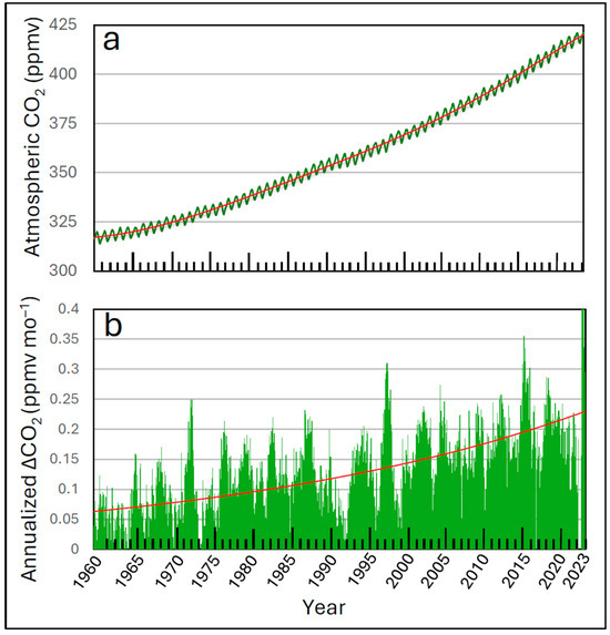
Figure 9.
Changes in atmospheric carbon dioxide (CO2) concentration (part (a)) and the rate of change in CO2 concentration (ΔCO2) computed monthly from running 12-month (annualized) averages (part (b)) over the last six decades. Absolute values (a) show seasonal fluctuations corresponding to seasonal photosynthetic variability, while the rate change of CO2 concentration (b) is dominated by the cyclic El Niño Southern Oscillation (ENSO). Part (a) shows the Keeling curve of the CO2 time series [358]. Part (b) replicates and confirms the ΔCO2 record in ([359], Figure 19, p. 21), recomputed here for a slightly broader timespan. The red line in (b) is the best-fit exponential trendline.
A marginally improved trendline fit to the Keeling Curve (r2 = 0.9949) is realized by a more complex sixth-order polynomial equation (red trendline in Figure 9a). The rate of increase in atmospheric CO2 concentration (ΔCO2) has also grown exponentially since 1960, increasing approximately threefold over the last 64 years (red trendline in Figure 9b). Since this excess CO2 is generally understood to originate from anthropogenic sources [20,22], it follows that humans continue to release CO2 to the atmosphere at an exponentially increasing rate in spite of warnings from scientists that this increase could damage the global environment irreparably.
Several global surface air temperature (SAT) and SST databases now exist, such as those collected and archived by the U.K. Meteorological Office (the HadCRUT5 dataset) [360]. Such widely-vetted databases show that global temperature increased in recent decades at variable rates, with El Niño Southern Oscillation (ENSO) cycles superimposed as a dominant short-term source of global temperature variance (Figure 10a). As expected from the proposed causal effect of global temperature on atmospheric CO2 concentration, temperature and CO2 are strongly and positively correlated (Figure 10b).
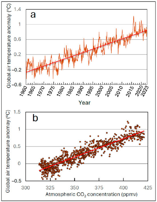
Figure 10.
Near-surface global temperature anomaly over land and sea in both hemispheres compared with the baseline years of 1960–1990 (part (a)) and its relationship with atmospheric carbon dioxide (CO2) concentration over the same time period (part (b)). The largest cyclic element visible in the temperature record (a) is the ~3-year El Niño Southern Oscillation (ENSO) cycle. Abbreviations: ppmv, parts per million by volume; °C, degrees Celsius. In part (b), the Pearson correlation coefficient r is 0.920 (sample size or n = 758, alpha level or probability, p = 0.0001, directional test). The red line is the best-fit linear trendline.
6.2. Rates of Change of Carbon Dioxide Versus Temperature
Comparing ΔCO2 (green bars in Figure 11) with ΔT (red bars in Figure 11) reveals a significant difference in their variation over time. Whereas ΔCO2 has increased exponentially since 1960 and continues to accelerate (Figure 9 and green bars in Figure 11), the growth curve of global near-surface temperature as measured by the peak amplitudes of El Niño events (largest red bars in Figure 11) increased from 1960 to 1976, flattened from 1976 to 1994, and then declined until the most recent El Niño (Figure 11).
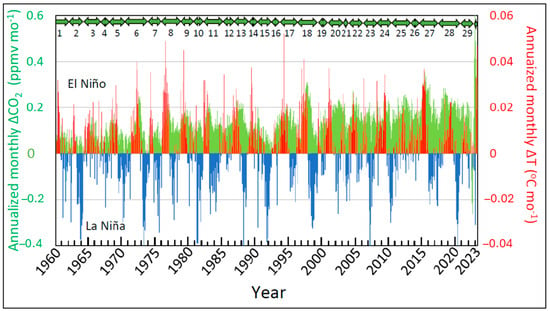
Figure 11.
Time series showing by month the rate of growth of atmospheric carbon dioxide (CO2) concentration (green bars) computed as running annual average over a 12-month period (“annualized”) and simultaneous rates of change in global temperature as reflected in cycles of the El Niño Southern Oscillation (ENSO). El Niño and La Niña are represented by red and blue bars, respectively. Original temperature data are from the U. K. Hadley Met Office, the HadCRUT5 dataset [360]. The annualized monthly rate of change in atmospheric CO2 concentration was computed similarly from the Keeling curve (Figure 9a). The green double-headed arrows across the top of the panel define individual CO2 rate cycles (numbered beginning in 1960), which are correlated with but lag the ENSO temperature cycle. This figure replicates and confirms ([359], Figure 19, p. 21) for the same but updated data.
These visual trends are evaluated for statistical significance in Figure 12. From 1958 to ~1976, the rate of global warming (ΔT) increased discernibly (r = 0.87, p = 0.001). The rate of growth peaked in 1976 and then declined slightly but non-discernibly for eleven years until ~1994 (r = −0.093, p = 0.393). Starting in 1994, ΔT declined discernibly until ~2021 (r = −0.607, p = 0.011). The temperature rate profile of peak El Niño events over the entire time range from 1958 to 2021 is summarized in Figure 12d. Peak El Niño rate of temperature change reached a multidecadal maximum almost five decades ago in 1976, remained flat for a decade, and then declined to 2022.
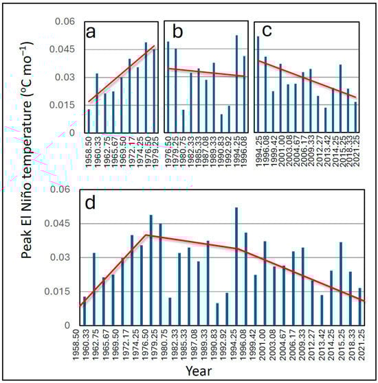
Figure 12.
Peak annualized running average of monthly rate of change in El Niño temperature maxima. (a), 1958–1979; (b), 1976–1996; (c), 1994–2001. See text for corresponding Pearson correlation coefficients. Red lines show best-fit linear trendlines for the corresponding data range (parts (a–c)) as integrated over the period 1958–2022 (part d). The rate of warming peaked in 1976, stayed flat until 1994 and then declined discernibly until 2021. Part (d) summarizes the continuous temperature growth rate profile since 1958. Compare these findings with the steady exponential growth of atmospheric CO2 concentration over the same time period (Figure 9). Based on the U. K. Hadley Met Office, the HadCRUT5 dataset [360]. Abbreviation: mo, month.
The same analysis performed on mean monthly El Niño temperature rate (Figure 13) rather than peak temperatures (Figure 12) increases the sample size by more than an order of magnitude, leveraging the statistical power of the HadCRUT5 database. This approach yields much the same result, namely peaking of global temperature in June of 1976 and a steady decline thereafter to March of 2021 (Figure 13). These interpretations require that any temperature change induced by emitted CO2 manifest quickly enough to appear on the decadal timescales of Figure 12 and Figure 13. There is apparently no empirical research on this question, but modelling studies cojoining the carbon cycle and physical climate models indicate that the temperature effect of emitted CO2 is fairly immediate, maximizes on average in 10.1 years, and within 90% probability limits as quickly as 6.6 years [361], well within the time windows evaluated here.
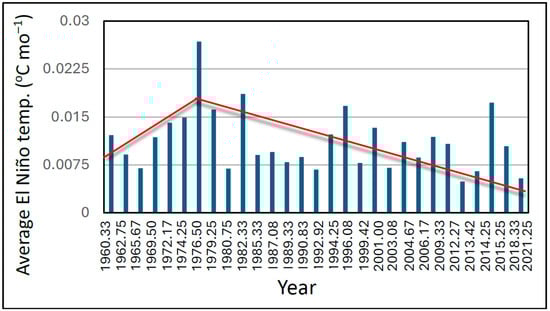
Figure 13.
Annualized running average of monthly rate of change in El Niño temperature averages (ΔT). The slope of the linear best-fit curves is discernibly positive from 1960 through 1976 (Pearson correlation coefficient or r = 0.76, directional p = 0.0248), but discernibly negative from 1976 through 2001 (r = −0.387, directional p = 0.034). Based on the U. K. Hadley Met Office, the HadCRUT5 dataset [360]. Abbreviations: temp., temperature; mo, month.
The conclusion that the global warming “Hiatus” began in 1998 and ended in 2012 therefore appears to be premature. Based on the global temperature measures used here, at least, the slowdown in ΔT started earlier and continues to the near-present. Many additional years and perhaps decades of data are required before a future prognosis can be accurately drawn within acceptable (95%) confidence limits [362].
These findings raise fundamental questions for contemporary climate science, beginning with the concept of climate response to CO2. Climate sensitivity to CO2 is defined as the temperature increase associated with a doubling of atmospheric CO2. According to theory, climate sensitivity is a constant that is described mathematically by the logarithmic curve of CO2 concentration vs. radiative forcing ([52], Figure 8) and is reported by the IPCC as a ~1.5 to 4.5 °C increase in temperature per doubling of CO2. By this standard definition, the ratio ΔT/ΔCO2 (=climate sensitivity) is in theory a constant.
In practice, however, the above instrumental climate data show that the ΔT/ΔCO2 ratio has varied by an order of magnitude over the last six decades based on the HadCRUT5 near-surface global temperature dataset [360] and the Keeling CO2 time series ([358], Figure 9a above). Assuming that both of these empirical datasets are valid, which is almost universally accepted by climate scientists, the discovery of order-of-magnitude variation in the ΔCO2/ΔT ratio presents a potential problem for the concept of climate sensitivity. The conclusion above that human-sourced CO2 was responsible for just 1.57% of global temperature forcing in 2020 (Figure 1) suggests the possibility that the sensitivity of the climate to CO2 is so low that variations are lost in the noise. Climate sensitivity has been a key concept of climate science, and clarification is recommended as a future research priority (Section 11).
The modern global near-surface air instrumental temperature record therefore shows that ΔT peaked in 1976 and declined thereafter until at least 2021 while at the same time the rate of growth in atmospheric CO2 concentration (ΔCO2) increased exponentially from 1960 to 2024. This finding, based on widely accepted empirical data, demonstrates that ΔCO2 did not cause ΔT. It is nonetheless clear from time series panels (Figure 11) that ΔCO2 and ΔT are strongly correlated and cyclic, with ΔT leading in phase [79]. Every El Niño cycle of the past 60 years was followed after a short latency by a train of monthly CO2 peaks that ended with the onset of the following La Niña (Figure 11). This timing is further evidence, in this case from the instrumental rather than the paleo record, that ΔT forces ΔCO2 rather than the converse.
The presumed mechanism of this causality is again the well-known greater solubility of CO2 in colder sea water [80]. As a consequence, each El Niño warming cycle is followed after a measurable latency by the release of CO2 from warmer sea water to the atmosphere. The measured mean delay from the peak cooling attained in each La Niña cycle in Figure 11 to the next peak CO2 increase is 9.76 months, confirming the comparable latency of 9–10 months [79] for the same data over the time period ending in 2012. These analyses provide an empirical estimate of timing dynamics for the transfer of CO2 from the oceanic to atmospheric reservoir when forced by a warming ocean.
Evaluation of both peak (Figure 12) and average (Figure 13) El Niño amplitudes yields a similar forecast for the future of the global climate. In both cases, the recent five-decade decline in the rate of warming extrapolates linearly to zero rate of change in ~2.7 decades. Zero rate of change in temperature implies zero growth in temperature, or temperature peaking, after which a half-century of global cooling is projected as the AAO enters its negative (cooling) phase (Section 8). It will require the passage of at least a decade, however, before the hypothesis that this decline in global warming rate is continuing can be evaluated confidently (p < 0.05) from empirical temperature data [362].
6.3. The Hiatus in Global Warming Rate
The above climate dynamics exemplify the well-known “Hiatus” or pause in the rate of global warming that was flagged and named by the IPCC in its Fifth Assessment Report [19]. The alternative term “Slowdown” has been suggested by some authors [363,364] and is used here interchangeably with “Hiatus.” Over the period of the warming Hiatus, the concentration of CO2 in the atmosphere increased exponentially (Figure 9a) as did its rate of growth (Figure 9b), while growth in the rate of warming declined (Figure 12 and Figure 13).
The discovery of the Hiatus led some to question the conventional wisdom that atmospheric CO2 causes global warming. As will be shown below, no extant hypothesis advanced to explain the rate Slowdown is inconsistent with continued climate forcing from any source, including atmospheric CO2, even though as shown in this review CO2 forcing is small compared with other climate drivers. The Hiatus has also presented a challenge for computer modeling of climate. At least forty widely used general circulation models are unable to predict or re-create the Slowdown [69], raising questions about the utility, accuracy and role of these models as applied to the Hiatus. The research interest inspired by the Hiatus is reflected by at least 865 peer-reviewed papers on the topic published since 1993 (Figure 14), most of which entail computer modelling rather than observational (empirical) studies.
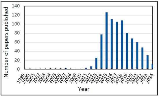
Figure 14.
The number of peer-reviewed climate science papers published from 1999 to 2024 that included the term “hiatus” in the title or abstract as retrieved using Google Scholar.
Of 89 peer-reviewed papers that placed specific dates on the beginning and end of the Slowdown, the mean start date was 1999.45 while the mean end date was 2011.93 (computed from ([363], p. 1856, Table 1 and Figure 1a, p. 1858)). The commonest date range reported for the Hiatus is 1999–2012 [364]. The 2012 end date was advanced in part because of the apparent temperature rebound associated with the record El Niño warming episode of 2015–2016 [365,366]. Depending on the rapidity of the observed change in global temperature, however, 10–20 or more years of continuous time-series data are needed to establish statistically-significant trends [362]. Therefore, describing the Slowdown as “ended” based on two or three years of time series data is not statistically justifiable [352,367].
Warming rate acceleration as of 2024 remains, statistically speaking, “not yet detectable” within generally accepted confidence limits for hypothesis testing (p < 0.05) [362,367]. From the year 2024, as many as 25 years of additional data may be required to detect a statistically significant change given current warming rates [362]. Applying this scientific standard to the Slowdown, the reduction in warming rate has persisted for at least 45 years (1976–2021) and shows no sign of abating (Figure 12 and Figure 13). The near-record El Niño event in 2024 has not yet been incorporated into this analysis. Its effect can be evaluated only when additional years or decades of continuous surface temperature data become available.
Several recent empirical studies of the Hiatus suggest its absence in high mountain environments [368,369] and on the Tibetan Plateau [370], raising the possibility that the global warming Slowdown is not homogenous across the globe. The Slowdown has nonetheless manifested strongly in lower elevations across China [371,372] and globally, supporting the hypothesis that the Slowdown is a worldwide phenomenon and not limited to near-surface global temperatures. The spatial distribution of the Hiatus and the reasons for any lack of geographical homogeneity are topics for further research.
Nearly a dozen candidate hypotheses have been advanced to explain the Hiatus. These include differences in the definition of the Slowdown [373], artifacts related to data biases [374], lack of statistical significance in time series cataloging the Slowdown [362], differences in datasets used to study the Slowdown [373], changes in stratospheric water vapor [375,376], increased aerosol concentration in the troposphere vented from volcanoes [377,378], “missing heat” implying redistribution of heat produced by ongoing radiative forcing by CO2 and stored somewhere in the ocean [373,379,380,381,382,383,384,385,386,387], cooling of surface waters in the equatorial Pacific [388], and natural climate oscillations including the Pacific Decadal Oscillation (PDO) [389,390,391] intensified by easterly winds over the equatorial Pacific [392,393] and the Atlantic Multidecadal Oscillation (AMO) [394,395].
Continuing research on the Hiatus has enabled provisional rejection of all but one of these hypotheses. Definitional differences [384] are resolved by the now-accepted general definition of the Hiatus as a reduction in the rate of warming, not reduction in its absolute value, both of which continue to grow (e.g., Figure 10 above). Data biases are countered by the robustness of the Slowdown across numerous well-accepted temperature databases ([373], Figure 1a). Lack of statistical significance [384] is addressed by studies showing statistically significant reductions in SST and SAT during the Hiatus [396,397] (Figure 12 and Figure 13 above). Modeling studies suggest that changes in water vapor in the stratosphere are insufficient to cause the reduction in ocean heat content (OHC) implicit in the Slowdown [398]. The largest single injection of water vapor into the atmosphere was caused by the eruption of a volcano in the Pacific Ocean off the island nation of Tonga on 25 January 2022, which caused increased regional warming, rather than the decrease in global warming rate associated with the Hiatus [399]. This volcanic venting occurred in any case a decade after the usually cited time course of the current Hiatus (1999–2012).
Aerosol accumulation in the atmosphere from volcanoes and consequent global cooling are unlikely to underlie the Hiatus because volcanic cooling effects typically peak within one year of eruption and subside within two years [400], while the Hiatus duration is several times longer. The most recent major volcano was Mt. Pinatubo, Luzon, Philippines, in 1991. No major volcano erupted during the period from 1999 to 2012, the previously accepted time window of the most recent Hiatus ([400], Table 1, p. 192).
As shown below, similar global warming Slowdowns occurred in 1940–1970 and 1870–1915. While there have been 13 “major” volcanic eruptions since 1783 ([401], Table 1, p. 192), none occurred within 2 years of the 1940–1970 Hiatus. That Hiatus therefore could not have been caused by volcanic venting. Six major volcanos erupted during the 1870–1915 Hiatus, however, including two of the largest on record (Krakatau, Indonesia, 1883, and Novarupta [Katmai], AK, USA, 1912). It is plausible and perhaps probable that the especially long (45 year) Hiatus in global warming rate from 1870 to 1915 was prolonged by aerosol-induced cooling associated with the then-concurrent flurry of volcanic activity. The current Hiatus, however, cannot be explained by volcanic eruption [377]. Portrayal of the Hiatus as a “rogue event” [402] based on computer modeling is inconsistent with the observed regular repetition of the Slowdown over recent centuries in empirical temperature records, and particularly with its phase-locking with the AAO for at least the last three cycles (reviewed below).
Two remaining hypotheses to explain the Hiatus are the “missing heat” or “heat redistribution” hypothesis [396,403,404], and the influence of the negative (cooling) phase of natural climate cycles like the PDO and AMO [405]. The “missing heat” hypothesis holds that temperature forcing by atmospheric CO2 has not slowed, but instead the excess heat imbalance (EEI) generated by presumed continued increasing CO2 forcing has been shunted to and stored within other, unidentified planetary heat reservoirs. The ocean is the most likely target reservoir for this storage because it contains more than 90% of planetary heat [406,407,408], but the atmosphere and cryosphere are also candidate CO2 reservoirs. This approach is compromised, however, by discrepancies in measurements of OHC across different databases [409,410].
The hypothesis of heat redistribution to the mixed layer of the shallow ocean (above 2000 m deep) is problematic for several reasons. Based on float data from the Array for Real-time Geostrophic Oceanography (ARGO), ocean heat content between 0 and 1900 m deep did not change appreciably from 2004, when ARGO records began, until 2012.5, when the Hiatus is widely described as already ended [111], ([359], Figure 23, p. 24, lowest panel). The weak increase that is recorded did not begin until around 2012, at the end of the usually cited 1999–2012 window for the Slowdown.
The hypothesis of heat transfer to the deep ocean is likewise problematic because heat from surface waters cannot be transferred quickly to the abyss. Most known oceanographic phenomena that distribute heat throughout the upper well-mixed layer are confined usually to above 700 m deep but no deeper than 1200 m [411]. These upper-layer mixing mechanisms include mesoscale and smaller eddies spawned by major western boundary currents in the open ocean [412,413,414], in regional seas such as the South China Sea [415,416,417] and the Arabian Sea [418], and in the SO surrounding Antarctica [419,420,421,422]. Both mesoscale and submesoscale eddies in Antarctica transfer heat upward, however, from deeper-water sources through the sea surface to the atmosphere [414,415,421,423]. Some classes of eddies transfer heat downward, but as a general rule ocean eddies do not transfer net heat to the depths.
The primary mechanism for redistributing heat to the abyssal ocean (1900 m and deeper) is the AMOC, which flows too slowly to explain the Hiatus in warming in shallower strata of the ocean. Heat cannot be transported to the depths of the ocean by the AMOC fast enough to account for the apparent “missing heat” at the surface. Finally, the AMOC itself may be slowing [332,424,425,426], which would be expected to delay heat transfer to the abyss even further and cause heat accumulation nearer the ocean surface.
Heat shunting to shallower, well-mixed water strata above the mean global ocean pycnocline (~2000 m deep) cannot account for the Slowdown, since sea surface temperatures (SSTs) have shown the same Slowdown as SAT [79]. This finding is expected, since global SAT is driven primarily by SST and oscillates with SST, which it lags in phase [79,427,428,429]. Heat accumulated in the well-mixed upper layer of the ocean increased from 2004 to 2022 based on ARGO float data ([359], Figure 25, p. 26), but this accumulation can be explained by other well-established oceanic mechanisms, including the slowdown of the AMOC [312,424,425,426] and internal climate variability imposed by various natural temperature cycles such as the PDO, AMO, and others (see below). Moreover, ocean temperature recorded in ARGO float data at all layers of the ocean from 2004 to 2021 show stability or moderate decline until 2009–2013, depending on water depth ([359], Figure 24, p. 25). These later increases in ocean temperature cannot reflect the “missing heat” invoked to explain the Slowdown as it has been understood conventionally, since the Slowdown began much earlier and by previous accounts ended by 2012.
Several authors have noted the difficulties in finding the missing heat postulated by this hypothesis [364,410]. The missing heat hypothesis in any case may not be a useful (falsifiable) scientific hypothesis for two reasons, one technical and the other intrinsic. The technical reason is that we do not currently have an adequate spatial or temporal understanding of OHC, particularly in the deep ocean, because requisite oceanographic observation platforms are not yet sufficiently developed and deployed [410]. Observational studies on OHC are currently infeasible because “…vertical heat transport is virtually impossible to measure on a global scale” [414] (p. 1), i.e., empirical analysis of vertical heat transport in the ocean on a global scale is beyond current technical reach.
The intrinsic flaw in the “missing heat” hypothesis, which has also been recognized by previous investigators [364] is that the global OHC is larger by many orders of magnitude than the missing heat required to explain the global warming Hiatus. Even if missing heat were systematically transferred to a different oceanic layer or basin, its magnitude is so much smaller than natural variance in OHC (estimated here as 0.000183% to 0.000935%; SM, part 4) that the hypothetical “signal” (i.e., the “missing heat”) cannot be distinguished from background noise. These percentages were computed for the Pacific Warm Pool (PWP), which is an extreme case because it is the largest body of warm water (>28 °C) anywhere in the global ocean. The percentages would be different for other oceanic regions.
The only remaining viable hypothesis to explain the Hiatus in global warming, therefore, is the cooling effects of natural climate cycles that have entered their negative phase of declining temperature [405,430] (see also below). The AAO hypothesized here to drive global climate oscillations such as the PDO and AMO has not been linked previously to the Slowdown as a cause, even though its repetition frequency for the last three cycles (73 years; ref. [143] falls in the middle of the range of the PDO, i.e., low-frequency modes up to 50–100 years [128,431,432] and the AMO, from 40 to 80 years [131] to a slightly longer 60–100 years [433].
Direct empirical evidence that the Slowdown is caused by natural variability of climate, typically the PDO/AMO, is reported in dozens of scientific papers authored by hundreds of investigators. Some of these studies identify only internal natural variability of climate as the cause [386,404,405,434,435,436,437,438,439]. Most of this extensive literature, however, explicitly identifies the cooling phase of the PDO and/or AMO as the immediate cause of the Hiatus [260,371,395,404,430,440,441,442,443,444,445,446,447,448,449,450,451,452,453,454,455]. In either case, the Hiatus is induced by the negative (cooling) phase of the corresponding natural climate cycle, explaining both the phasing of the Hiatus and its recurrence over time on an approximate 60–80-year cycle. Ollila [456] aptly summarized the mechanism of the Hiatus as follows:
“When the oscillation phases changed to negative phases, the cooling effect of the 60- & 88-year oscillations became dominant … and caused global temperature to decrease, which happened from 1940 to 1975. Similarly, when the 60- & 88 [-year] oscillations turned from a negative to a positive phase, global warming accelerated, as it did after 1975 and finally increased the global temperature by about 0.25 °C (Figure 6) till [sic.] 2000.”[456] (p. 306)
If the Hiatus is caused by the cooling phase of the AAO, then these events would be expected to coincide, which they do for past Slowdowns (Figure 15). The present Hiatus, however, began during the latter warming phase of the AAO. Answers may lie in phase relationships between the AAO, PDO and AMO. The recent discovery that the loss of sea ice in the Arctic has slowed during the last two decades [209] is consistent with a common cause, the AAO.
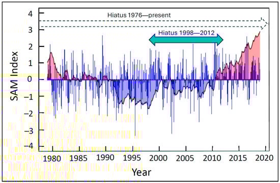
Figure 15.
Time series of the Antarctic Oscillation (AAO), measured here by the Southern Annular Mode (SAM) index, plotted on the same panel as the global warming Slowdown (Hiatus). Two alternative Slowdown scenarios are shown, the most commonly cited (1998–2012, blue double-headed arrow), and the longer Slowdown proposed here based on the rate of change in temperature (open dashed arrow). The cumulative SAM index is shown by the solid black curve, with red and blue fill corresponding to the positive and negative phase of the AAO, respectively, while blue bars mark the SAM index time series. The SAM index is based on ([41], Figure 2b, p. 4).
Attribution of the Hiatus to the cooling phase of natural climate cycles (the AMO, PDO), while supported by the extensive evidence summarized above, is in practice a minor variation on the theme of the “missing heat” hypothesis [457]. Both hypotheses entail redistribution of heat within the Earth’s climate system, differing only in the mechanism of redistribution and perhaps the final storage site of the missing heat. The natural climate cycle elaborated here explains the missing heat by the operation of this cycle rather than by other, unidentified oceanic mixing forces, irrespective of the magnitude of any continued ΔRFCO2. In particular, and contrary to some interpretations, the occurrence of the Hiatus is consistent in theory with ongoing simultaneous climate forcing from any source, including atmospheric CO2. As this review highlights, however, CO2 forcing of climate is in practice small in comparison with natural variability in global temperature as driven by the AAO.
Instrumental temperature records from several sources demonstrate that the contemporary Slowdown in the rate of global warming is not unique in recent climate history (Figure 16). Homologous Slowdowns occurred in 1870–1915 and in 1940–1970 [206,458,459], separated by intervening warming periods or temperature “surges.” The global warming Hiatus is part of a recurrent, long-term natural cycle (Figure 16) that entails cooling of surface waters in the Tropical Pacific [388,405,443,460] driven presumably by Ekman pumping from the SO. Both Slowdowns and subsequent warming surges are coupled with the AAO. The most recent three Slowdowns coincide approximately with the peaking and negative (cooling) phase of the AAO, while the intervening warming periods are coincident with the positive (warming) phase of the AAO (Figure 16).
The conclusion that current global temperatures do not comprise a statistically measurable warming surge [362] implies that, as proposed above, the global warming Slowdown has not yet ended. These findings collectively suggest a continuing Hiatus in global warming that is phase locked with the AAO and potentially coupled with it causally. As noted, however, the existence of a recurrent Slowdown or Hiatus in global warming rate does not imply that CO2 forcing stops during those Slowdowns, even though as documented in this review, such CO2 forcing may be itself be too small to detect. In this interpretation, the Hiatus represents a redistribution of global heat from all sources, including CO2 forcing, caused by mainly by natural climate variability, the AAO.

Figure 16.
Coincidence of global warming Hiatus’ (double-headed arrows at top) with the cooling phase of the Antarctic Oscillation (AAO) as portrayed by the Southern Annular Mode (SAM Index). Modified from ([206], Figure 2c, p. 448). Vertical lines signify statistically-discernible linear trends at the indicated data points (p < 0.05).

7. The Coupled Oscillator Hypothesis of Global Climate
The above exploration of the Hiatus highlights coupling between three of the participant natural climate cycles, the AAO, PDO and AMO. The most basic criterion for cycle coupling is oscillation at common or harmonic frequencies. As noted above, these three cycles all show overlapping periodicities at 60–80 years. A second criterion is that the cycles exhibit similar or at least relatable time series profiles. Superimposition of these three natural climate cycles reveals the similarities in their respective patterns of warming and cooling (Figure 17) [41].
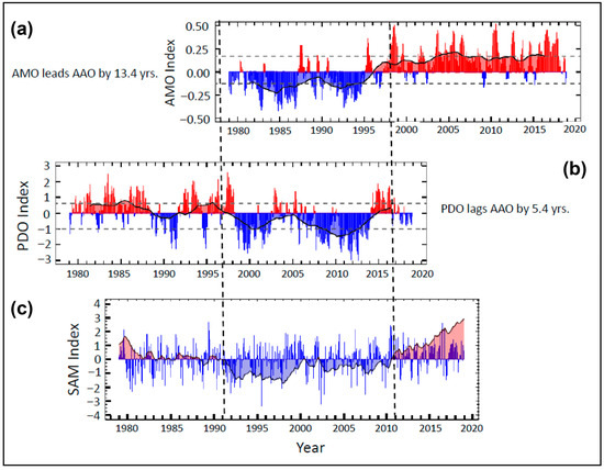
Figure 17.
Three natural climate cycles shifted in time relative to each other to align similar patterns of temperature fluctuation, from which time lags from the Antarctic Oscillation (AAO) are estimated. The three natural cycles shown are the AAO (Southern Annular Mode, or SAM index, bottom panel), the Pacific Decadal Oscillation (PDO, middle panel), and the Atlantic Multidecadal Oscillation (AMO, top panel). In parts (a,b), red and blue bars indicate warming and cooling events associated with El Niño and La Niña respectively. Black lines represent cumulative (average) indices of the corresponding cycles. In part (c), blue bars show the SAM index time series while the black line signifies the cumulative SAM index measured at the ERA-interim 500 hPa level. Red and blue shading indicate warming and cooling phases, respectively. See text for comparisons. The bottom, middle and top panels are, respectively, from ([41], Figure 2b, p. 4, Figure 9b, p. 13, and Figure 10b, p. 14).
Substantial empirical evidence suggests that the AAO is connected with the ENSO cycle and other modes of tropical temperature variability, including the PDO [40,165,461,462,463,464,465,466,467,468,469] and AMO [131,139,470]. The AAO is coupled also with more northerly cycles like the Arctic Oscillation [471] and the Aleutian Low [150] that extends over North America and has also been termed the Pacific-North American pattern [472,473].
Recent evidence suggests a complex connection between the AAO and both Pacific and Atlantic ocean basin cycles [394]. Proxies of the AAO are positively correlated with the PDO but negatively correlated with the AMO [40]. The phase shifts evident in Figure 17 suggest as a first approximation that the AAO precedes the PDO by 5.4 years but lags the AMO by 13.4 years. These independent findings suggest a direct AAO coupling with the PDO, but a potentially more complex, reciprocal, nonlinear and variable phase relationship with the AMO. Consistent with this conjecture, the lead-lag relationships between some of these cycles, notably the PDO, AMO, NAO and Southern Oscillation Index (SOI) or ENSO cycle, vary systematically on specific cyclic periods ranging from a 13-year AMO-PDO lead to a 17-year AMO-PDO lag [403].
Faster decadal oscillations such as the ENSO, can potentially be understood in the CO hypothesis as harmonic derivatives of the above centennial cycles. Intra-seasonal cycles such as the Madden-Julian Oscillation may be harmonics of decadal oscillations. In the CO hypothesis these global and regional climate cycles are all forced by the primary pacemaker, the ACWO wind cycle and the accompanying AAO temperature cycle, which originate in the most energetic corner of the globe, the SO near Antarctica, and serve as the proximate driving force of global climate on centennial and millennial timescales. The relation between the AAO and other natural climate cycles distributed across the globe is amenable to quantitative methodologies developed for the analysis of coupled oscillators [158,474,475,476,477,478,479,480,481,482,483]. Confirmation and further documentation of the coupling of “follower” climate cycles to the “pacemaker” oscillator in the SO, the AAO, would comprise a significant advance in our understanding of global climate and is recommended as a priority target for further research (Section 11).
8. Empirical Projection of Global Climate
Predicting future climate has long been recognized as a guiding goal of climate science [484] and has been described as “both necessary and possible” [485]. Climate forecasting is widely appreciated as critical for policy decisions in sectors as diverse as preparation for extreme climate events [486], land management and agriculture [487,488,489,490], energy policy and distribution [491], tourism [492], public health [493], and wildfire management [494]. Given the pervasive influence of climate on human affairs, the capacity to predict climate accurately could benefit virtually all sectors of human activity.
8.1. Methodology
Most efforts at climate forecasting to date have entailed projections of future climate using theoretical computer models, including CMIP5 model simulations [495]. Computer forecasts have been restricted initially to decadal projections [496] and have demonstrated “limited” skill [497], particularly within the standard 95% confidence limits [498]. Recent advances in Artificial Intelligence (AI) have enabled data-driven hybrid models [499] and climate prediction using machine learning [500,501]. As noted above, longer-term projections using Earth System computer models are compromised by their incapacity to replicate the most basic and universal feature of climate, oscillation (Section 3.1).
Empirical projections of climate are beginning to emerge [40,502,503] based on extrapolating into the future the same stereotypic pattern of natural climate variability that has repeated reliably in the past. One of the most advanced of these efforts is a long-term program to predict Antarctic and SH climate based on empirical climate parameters of the past, including ice core sodium (a proxy for marine air intrusion) for the past 2000 years. On this basis the authors propose that near-term (decadal) climate forecasts are “plausible.” [40].
8.2. Global Climate Forecasts Based on the Antarctic Oscillation
The same methodology pioneered in the above studies on regional climate forecasting can be extended to long-term global climate based on the past behavior of the AAO. The first step is to establish the Earth’s current phase position in the AAO climate cycle and then extrapolate from the present the corresponding AAO pattern of the past into the future. For example, using only the information contained in Figure 4, Figure 5 and Figure 8 of this review, global climate of the future can be forecasted on timescales ranging from decadal through millennial for literally hundreds of millennia into the future. This enables answering key scientific questions that are prerequisite to informed, long-term public policy decisions, such as: When will the next cold trough occur? How long will it last? How cold will it get? When is the next warm peak, the next RWP (homologous with the MWP) and RCP (homologous with the LIA)? Answers to these and related questions about the climate of the future are essential to adaptive, science-based climate policies.
Beginning with the past, as well-established and illustrated in Figure 8, the LIA started in ~1303 of the CE and ended in ~1850 CE and was therefore ~547 years in duration. The mean duration of the most recent AIM cycle is 1050 years (Figure 8). Forecasting at this early stage in the model’s development assumes that the current AIM cycle is the same duration as the previous one, in which case the next LIA is projected to begin in the year 2353 CE (1303 + 1050) and end ~547 years later, i.e., in the year 2900 CE. These empirical projections based on the AIM cycle and the embedded LIA establish our present position in the millennial climate oscillation and the timing of the next RCP, or LIA homolog.
As shown above, climate of the past is organized into repeating millennial units in which Antarctic winds and corresponding temperatures undergo 6–8 centennial-scale oscillations that summate and facilitate throughout each cycle (Figure 5). Since the next LIA is projected to occur in 330 years, and assuming a mean AAO cycle duration of 100 years, ~3.3 centennial cycles remain in the current millennial segment of the global AAO “climate clock.” These projections imply that we are near the peak of the current centennial AAO cycle and have entered into the more prolonged millennial RWP homologous with the MWP. Following the pattern of the past, global temperature is projected to begin to decline in the near future for up to a half-century, corresponding to the negative (cooling) phase of the centennial AAO climate cycle, and then pass through at least three additional complete and ever-larger warm/cool cycles before culminating in the next RCP (a new little ice age) in approximately 3.3 centuries.
This empirical climate model based on the AAO therefore projects that global temperature will fall and rise again to a new maximum at least three times before the onset of the next RCP. Assuming that current global temperature coincides with the peak of the AAO and that AAO cycles are 100 years in duration, future recurrent global temperature peaks assuming a centennial cycle are expected at approximately 100, 200 and 300 years from the present, while global temperature troughs are expected approximately 50, 150, 250, years from now. For the remainder of the current AIM cycle, therefore, global temperature peaks are projected for approximately 2123, 2223, and 2323, in preparation for the next RCP, or LIA homolog.
Under these same assumptions, global temperature troughs are projected for the years 2173, 2273, and 2373, with the latter corresponding to the start date of the next RCP, or LIA homolog. If the projections are adjusted to account for the current warming cycle peaking in 2.7 decades (forward extrapolation of instrumental temperature trends from Figure 11 and Figure 12), these projections are advanced by 27 years, i.e., global temperature peaks are projected for 2150, 2250 and 2350 CE, while global temperature troughs are projected for 2200, 2300 and 2400 CE. These projections change if the mean duration of ACO cycles is shorter, 60–80 years, as currently reported (op. cit.).
Unlike previous computer-based projections of future climate, the above projections are based solely on widely accepted empirical climate data gathered independently by thousands of climate scientists, vetted repeatedly, and reduced and analyzed using the most basic statistical methods. These empirical climate projections require only two assumptions: climate of the next few centuries will follow the same pattern observed for at least the past 226 millennia, and the additional CO2 humans have emitted to the atmosphere will not alter these natural patterns substantially. Both assumptions are supported by the empirical evidence reviewed here.
These quantitative projections of global climate are preliminary and approximate for at least three reasons. First, the exact date of the peak in the present AAO is not yet known with the requisite 95% confidence. Second, current projections do not incorporate natural variance in relevant climate parameters (cycle period, duration and amplitude). Third, and related, these projections assume a mean AAO cycle duration of 100 years, while analysis of period variance may reduce this estimate to the currently reported 60–80 years. When empirical climate projections can realize 95% or greater confidence limits, they will meet a minimal scientific threshold for incorporation into climate policy.
The empirical climate projections exemplified here carry at least two advantages over theoretical computer models or hybrid AI models: transparency and replicability. Transparency arises because empirical climate projection is based on well-accepted observational data analyzed using basic statistical methods and therefore can be replicated by most graduate students in climate science. The resulting climate projections are therefore available to a greater fraction of the climate science and policy communities, as well as to the public at large, than are current projections based on comparatively arcane, uncertain and demonstrably-incomplete computer models. The empirical projections are correspondingly easy to replicate, which is helpful for achieving scientific consensus and fostering public confidence in climate forecasting.
Empirical climate models including the one proposed here have the potential to excel and surpass in five qualities deemed most important for climate projection using models [504], namely, (1) solution accuracy, (2) effectiveness of uncertainty quantification, (3) time-to-solution, (4) energy- or money- to solution, and (5) robustness (e.g., numerical stability). Ultimately, it may be reasonable to anticipate long-term climate predictive powers (centennial/millennial) similar to those now achieved with 3–5-day numerical weather forecasting, namely, up to more than 90% accuracy for 500 hectopascal geopotential height fields in the NH [500,501,505].
9. Mass Extinctions of Biodiversity
The empirical evidence reviewed above supports the hypotheses that global climate is driven primarily by a natural PWT cycle in the SO, the AAO, and that human-sourced CO2 in Earth’s atmosphere provides a small fraction of climate forcing, estimated here as 1.57%. The “other CO2 problem” [506] is acidification of the global ocean. Atmospheric CO2 dissolves at the air–sea interface to produce carbonic acid, which lowers the pH of the ocean (OA) to kill the plankton that collectively generate as much as 70% of planetary oxygen [47].
9.1. The Role of Atmospheric Carbon Dioxide
Numerous students of the fossil record have concluded that past mass extinctions were caused by the release of CO2 to the atmosphere, which destroys biodiversity through ocean acidification, plankton die-off, and global anoxia [23,507,508,509,510,511,512,513,514,515,516,517,518,519,520,521,522,523,524]. Genus loss has accordingly been strongly and positively correlated with atmospheric CO2 concentration for at least the past 210 My (Figure 18a), the most highly resolved segment of the 425-My paleo data record of atmospheric CO2 concentration [23].
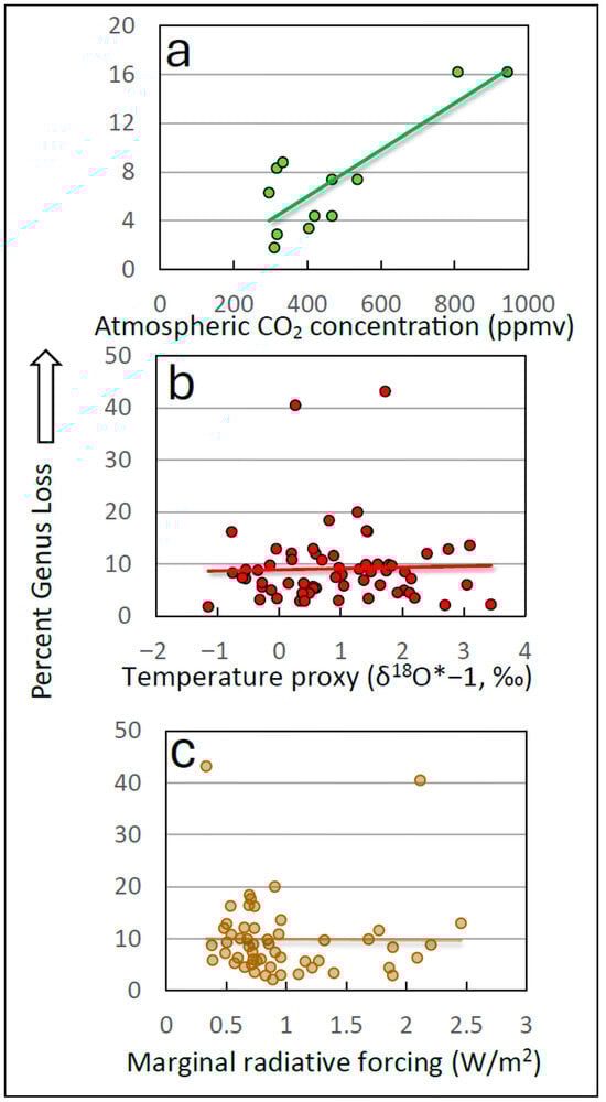
Figure 18.
The relationship between precent genus loss measured from the fossil record over the last 33 million years (My) (part (a)) and over the last 210 My (parts (b,c)) [525] and (a) the atmospheric concentration of carbon dioxide (CO2) [53], (b) long-term global temperature [54], and (c) marginal radiative forcing of temperature by atmospheric CO2 computed using MODTRAN [53]. Lines in each graph are best-fit linear trendlines. The respective Pearson correlation coefficients and corresponding alpha levels (“probabilities”) are: (a), r = 0.84 (p = 0.0006); (b), r = 0.03 (p = 0.80); (c), r = −0.001 (p = 0.80). From [23].
The contemporary effect of atmospheric CO2 on global biodiversity can be estimated from the fossil record by regressing past atmospheric CO2 concentration against percent genus loss. The regression yields a strong positive correlation of r = 0.84 over the most recent portion of the fossil record, the last 33 My (Figure 18a), when planetary geography and environmental conditions were most similar to those of today [23]. The CO2/extinction correlation when extended to include the last 210 My is r = 0.63 [23]. Using either regression demonstrates that today’s atmospheric concentration of CO2, as elevated by human activities to the current ~422 parts per million by volume (ppmv), is associated with a 6.39% genus loss. Judging from the fossil record, therefore, human emissions of CO2 may have already caused a significant extinction of global marine biodiversity, i.e., the Earth may currently be experiencing an ongoing mass extinction that is attributable to human activities and specifically to anthropogenic emissions of CO2 to the atmosphere.
9.2. The Role of Climate Change
While mass extinctions are directly proportional to atmospheric CO2 concentration, biodiversity loss is not discernibly correlated with long-term (My) global temperature (climate) (Figure 18b) nor with marginal radiative forcing of temperature by atmospheric CO2 (ΔRFCO2) (Figure 18c). It follows that long- term climate (temperature) change is not a major immediate cause of past mass extinctions at My timescales. Instead, more than two-thirds of variation in extinction rate (70.56%) is explained by variance in the atmospheric concentration of CO2 (r = 0.84, r2 = 0.7056, Figure 18a).
The proximate mechanism of the ongoing SME of marine life is inferred to be the same as for natural mass extinctions of the past, namely, acidification of the ocean by atmospheric CO2, which kills plankton that generate most atmospheric O2. Plankton mortality in turn depletes atmospheric O2 to create global anoxia that asphyxiates most higher life forms. Past natural mass extinctions, however, developed over a time period measured in millions of years. In contrast, the ongoing SME started with the onset of the Industrial Revolution in approximately 1750, when atmospheric CO2 concentration was still in the low-risk range, 280–300 ppmv (Figure 19, green arrow in lower left). Human-induced emissions of CO2 have raised the atmospheric concentration of CO2 by more than half in the geologically short span of 275 years, many orders of magnitude faster than natural mass extinctions of the past (Figure 19). At this rate, the SME will have mostly run its course by the turn of the next century (Figure 19).
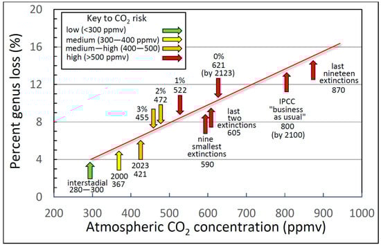
Figure 19.
Extinction curve showing computed risks to biodiversity associated with atmospheric CO2 reduction targets and milestones. The red curve shows the relationship between percent genus loss and atmospheric CO2 concentration based on the most recent fossil record (the last 33 million years). Downward arrows above the extinction curve show the annual percent cuts required to achieve the stabilization of atmospheric CO2 concentration over the next several decades at the levels shown in parts per million by volume (ppmv) (target dates are reported in [23]). The upward arrows beneath the extinction curve mark CO2 concentration milestones, starting with interstadial atmospheric carbon dioxide (CO2) concentrations between recent Great Ice Ages (green arrow at lower left) and culminating in the mean atmospheric CO2 concentration of the last 19 mass extinctions over the last 210 Myr (red arrow at upper right). This extinction curve suggests that the loss of biodiversity associated with elevated atmospheric CO2 is already occurring and will strengthen exponentially in the near future unless carbon emissions are curbed. The units of all numbers except percentages and dates are ppmv. Abbreviation: IPCC, Intergovernmental Panel on Climate Change.
9.3. Auto-Extinction of the Human Species
The extinction literature typically focuses on the projected effects on biodiversity, in general, or specific flora or fauna in particular (“endangered species”). References to the human prospect seldom appear, perhaps in part because the linkage between extinction, atmospheric CO2 and human activities has only recently been clarified. Diverse and independent evidence from many investigators now suggests that the proximate trigger for most and perhaps all past mass extinctions was a periodic increase in the concentration of CO2 in the atmosphere, which acidified the ocean and killed phytoplankton that generate up to 70% of planetary oxygen [47] to create a global anoxia that smothered life [23]. The CO2 currently emitted by human activities presumably has the same effect at similar doses. In this case, as plankton mortality causes free oxygen to decline, the partial pressure of oxygen (ppO2) in the atmosphere is expected to drop proportionately (Figure 20).
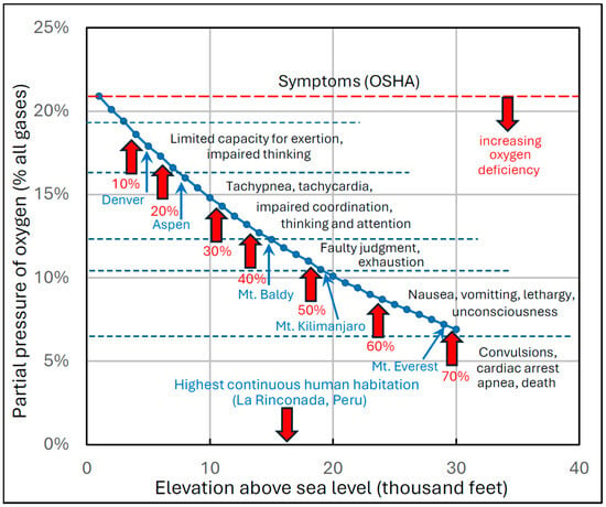
Figure 20.
Implications of the extermination of plankton and resulting anoxia induced by anthropogenic carbon dioxide (CO2) emissions and consequent ocean acidification. The solid blue curve shows the current relationship between altitude and the partial pressure of oxygen (ppO2) in the atmosphere expressed as a percentage (%) of all atmospheric gasses (original data plotted are from [526]). Black font above the blue curve on its right describes symptoms in humans of sudden (non-acclimatized) exposure to the corresponding ranges of oxygen (O2) deficiencies marked by horizontal blue dashed lines, as enumerated by the U.S. Department of Labor, Occupational Safety and Health Administration (OSHA) [527]. The acute symptoms listed in the figure are cumulative as O2 deficiency increases. Blue upward arrows designate current partial pressure of oxygen (ppO2) at the different geographical locations and altitudes identified by blue font. Red upward arrows designate percent O2 deficiencies associated with loss of the indicated percentages of atmospheric O2 from global marine primary production by phytoplankton up to the maximum 70% [47].
The ppO2 at sea level is currently ~20.9% of the partial pressure of all atmospheric gases. As altitude above sea level increases, ppO2 declines to 6.9% of sea level values at an elevation of 29,032′ (8849 m), the altitude of the tallest mountain on Earth, Mt. Everest (Figure 20). If anthropogenic emissions of CO2 eradicate 50% of the global plankton population that in turn generates up to 70% of atmospheric O2—which has happened repeatedly during the largest natural mass extinctions of the past—then the ppO2 in the atmosphere at sea level expressed as a percentage of all gases would drop to 10.45% of contemporary sea level values, approximately the ppO2 today at the top of Mt. Kilimanjaro at an elevation of 19,341′ (5895 m) above sea level (Figure 20).
The highest altitude at which humans currently live continuously is the mining community of La Rinconada in the Eastern Andes at 16,732′ (5100 m) above sea level, where highly acclimatized Peruvians survive precariously at a ppO2 of 11.6% of contemporary sea level values. If anthropogenic emissions of CO2 were to eradicate all oceanic plankton, ppO2 at sea level would drop to ~6.9% of current sea level values, similar to that at the top of Mt. Everest today at an elevation of 29,032′ (8849 m) (Figure 20). Neither humans nor most mammals, birds and even reptiles and amphibians could survive at such a depressed ppO2. Unabated human emissions of CO2 therefore imply the plausible extinction of most complex life on Earth from suffocation by the year 2100. The risk is magnified for large, O2-intensive homeotherms such as human beings.
9.4. Sensitivity of Contemporary Phytoplankton to Ocean Acidification
The hypothesis developed above that human-sourced emissions of CO2 threaten human extinction from OA is based on the fossil record, which projects a 6.39% decline in contemporary marine genera at today’s atmospheric CO2 concentration [23]. If this hypothesis is accurate, corroborating evidence should be available from plankton populations living in today’s moderately-acidified ocean. The evidence is reviewed in this section, organized around three questions: (1) is OA harming contemporary phytoplankton? (2) is phytoplankton abundance therefore declining? (3) is the atmosphere showing any corresponding sign of reduced ppO2?
The first of these questions has stimulated intense research interest, evidenced by thousands of peer-reviewed publications since 2000. Most of these studies employed laboratory or ship-deck plankton cultures in which independent variables like pH could be controlled. Early studies yielded mixed and often confusing outcomes [528,529]. Results were sometimes contradictory even when addressing similar questions and working with the same species [530]. One research group reported no effect of CO2 on photosynthetic rate in the picocyanobacterium Synechococcus [531] while an independent study on the same genus and strain reported reduced growth rate at higher CO2 (lower pH) levels [532]. Some Arctic phytoplankton showed resistance to OA at the level of individual cells [533], but exhibited changes in community structure [534,535], while other Arctic phytoplankton communities experienced a 50% reduction in growth rate in response to a pH decline from 8.0 to 7.1 in laboratory cultures [536]. Some Antarctic phytoplankton species show positive growth responses to increased CO2, while others show reduced growth [537]. According to one earlier review, “photosynthetic responses to OA are relatively small for most investigated species and highly variable throughout taxa.” [531].
Some of this variance may originate from the use of different experimental protocols [530]. Another source of variance may be intrinsic to the widely used experimental protocol, especially in laboratory and ship-deck cultures, of bubbling CO2 at known concentrations through sea water to acidify it. The acidified sea water can damage phytoplankton (the cost), and simultaneously provide carbon as a photosynthetic substrate, raising primary production by carbon fertilization (the benefit). The “tipping point” between these opposing influences is realized when the cost outweighs the benefit and the experimental population dies or the taxon becomes extinct. The same balancing act presumably characterizes natural phytoplankton ecosystems.
Whether cost of CO2 exposure outweighs the benefit of carbon fertilization varies depending on the species or strain of phytoplankton and a host additional variables and stressors [538,539,540], including temperature [541,542,543,544], water depth [545], cell size [546,547], UV-light exposure [548,549], nutrients [550], pollutants [539], plankton community structure [551], time [552,553], bloom stage for blooming phytoplankton [554,555], and the frequency of temperature fluctuations [556]. Even when OA has no apparent effect at the species level, undetected shifts in community structure can compromise long-term survival and primary production by phytoplankton [557].
A potential source of past variance in phytoplankton studies is the recently-discovered “phycosphere,” a thin extracellular aqueous layer enclosing individual plankton cells [558]. Within the phycosphere pH is metabolically maintained at values up to 0.41 ± 0.4 pH units higher than the bulk ambient sea water (pH = 8.00) that contains them [558,559,560,561,562,563]. This discovery potentially complicates the interpretation of some past experiments in which CO2 was controlled and measured only for the bulk sea water containing the phytoplankton, perhaps accounting for some of the variance in past results.
Past experimental variance may also related to the duration of experiments. Plankton can in principle adapt rapidly to adverse environmental conditions because they have short generational times (days) and therefore can evolve quickly [564,565]. In the well-studied pentate diatom P. tricornutum, OA enhances growth over the short term (tens of generations; [566]) but reduces growth over the longer term (1800 generations; [567]). A meta-analysis of 49 studies combined with modeling suggests that harmful effects of pCO2 on phytoplankton may take many generations to manifest and can therefore be missed in short-term (<2 weeks) experiments [553,568]. OA in coastal plankton communities has had a “devastating but reversible” impact [569].
Mesocosm experiments, in which large enclosures usually suspended in sea water harboring phytoplankton populations are exposed to controlled variables under quasi-natural conditions, are a logical step between laboratory incubation and field studies. While promising in concept, mesocosm experiments have yielded variable and sometimes contradictory results [543,570,571,572]. Several possible explanations for the differences have been advanced [573,574,575,576]. More recent mesocosm studies have reported adverse effects of OA more consistently [553,554,577], perhaps signifying better experimental control of the many potential confounding variables in these complex and little-known marine ecosystems.
The “tipping point” for the transition from benefit to cost, from survival to the extinction of phytoplankton, can be measured as the atmospheric concentration of CO2 at which the species or population becomes functionally extinct. This tipping point is estimated for one large group of phytoplankton, the coccolithophores, as ~600 ppmv [578]. If this estimate is accurate, then at today’s rate of increase in atmospheric CO2 concentration (~2 ppmv y−1; op. cit.), all coccolithophores will become extinct by 2114, eliminating 20% of marine primary production (see below). If similar tipping points characterize all phytoplankton, which is unlikely but unknown (see below), a mass extinction event initiated by phytoplankton loss would be plausible in less than a century.
More recent literature on the effects of OA on phytoplankton species and populations suggests greater consensus on at least some key questions. Among the several phytoplankton groups, diatoms contributed ~50% of total phytoplankton primary production between 1998 and 2011, equivalent to ~20 picograms per year of fixed carbon (PgCyr−1) [579]. Diatoms are encased in siliceous shells that are minimally impacted by OA, but many species nonetheless show degraded biological responses to OA [531,546,580,581,582,583]. Model simulations suggest that projected future ocean acidification could trigger an overall 13–26% decline in the oceanic diatom population by the year 2200 [584]. Dinoflagellates, a smaller group of phytoplankton that can dominate biomass in stratified warmer ocean waters, are also vulnerable to OA because their flagella are disabled in acidic environments and the organisms therefore lose mobility. The immobility induced by OA blocks the daily vertical migrations essential to dinoflagellate survival and the broader functioning of the pelagic ecosystem [555,585].
After diatoms, coccolithophores are the most prevalent and impactful phytoplankton groups in many marine environments. From 1998 to 2011, coccolithophores contributed ~20% of marine primary production [579]. Coccolithophores are especially vulnerable to OA [586] owing to their calcium carbonate (CaCO3) exoskeleton. OA at low levels induces aberrant skeletal elements (coccoliths), associated with impaired cellular function [528,529,587,588,589,590,591,592,593,594,595,596,597,598,599,600,601,602] and weakened resistance to copepod predators [603]. OA at higher levels dissolves the coccolithophore exoskeleton, killing the plankton [529,531,548,589,591,592,593,594,604,605,606]. Of all phytoplankton groups, evidence for an adverse effect of OA is strongest and most consistent in coccolithophores.
Diatoms and coccolithophores together comprise 70% of phytoplankton species. Among remaining marine phytoplankton, chlorophytes (green algae) are a larger group than diatoms and from 1998 to 2011 contributed ~20% of total marine primary production [579]. Many chlorophytes are calcifers, and these green algae groups are as vulnerable to OA as coccolithophores [607]. The majority of chlorophytes are non-calciferous. Some of these species show adverse effects from OA [608,609] although other studies record no effect or a positive stimulus on growth by high pCO2 [610] or rapid adaptation to low pH near deep-sea CO2 vents [611]. Some studies showing a positive effect of OA on growth, however, were short-term (2 weeks or less), leaving open the question of whether later generations might show degraded responses to OA. Additionally, the common sea grass Ulva sp. grows faster in lowered pH, but growth is inhibited by adding natural variables such as fluctuating light [612]. Cyanobacteria represented about 10% of primary production between 1998 and 2011 [579]. Some members of this group play the crucial ecosystem role of nitrogen fixation, and many are degraded by OA [581,613,614,615,616].
The first question posed above, whether OA harms living plankton populations, can therefore be answered in the affirmative with qualifications. Early studies yielded mixed and sometimes contradictory results, but more recent studies support the hypothesis that ocean acidification at today’s level broadly damages living phytoplankton, and that further OA will cause increasing phytoplankton harm, species loss and community disruption, with corresponding reduction in marine primary production. Coccolithophores and calciferous chlorophytes are probably most acutely endangered by increasing OA while remaining groups are generally at least partially impaired. A recent review of 985 studies concluded that “…many calcifiers (e.g., echinoderms, crustaceans, and cephalopods) are found to be tolerant to near-future ocean acidification (pH ≈ 7.8 by the year 2100), but coccolithophores, calcifying algae, and corals appear to be sensitive. Calcifiers are generally more sensitive at the larval stage than adult stage. ” [617] (p. 1). For marine biodiversity, phytoplankton serve as “leading indicators” of potential global ecosystem damage. Better understanding and monitoring of natural plankton populations is therefore recommended (Section 11) as a future research priority.
The second question posed at the beginning of this section, whether plankton abundance is decreasing in today’s ocean, has been addressed by field studies aimed at assessing the status of current living plankton communities. Field sampling of phytoplankton populations suggest that their abundance has declined in eight of the world’s ten major ocean regions [618,619,620,621]. By one extreme estimate, phytoplankton concentration declined over the past century at an estimated rate of ~1% yr−1 [618]. The abundance of oceanic phytoplankton reportedly fell by 40% from 1950 to 2008, a period of the largest and fastest increase in atmospheric CO2 concentration in recorded human history. Some observers attribute the decline in plankton abundance to climate change [622], which remains a possible contributor, but phytoplankton mortality from increased ocean acidity is well documented (op. cit.). Whatever the cause(s), it appears likely that anthropogenic emissions of CO2 are already adversely impacting the oxygen-producing capacities of global ecosystems.
The third question posed above, whether contemporary atmospheric oxygen is declining, is addressed by the Scripps Institute, which estimates that atmospheric oxygen concentration has declined by an average of 4 parts per million by volume for the last 25 years ([623], Figure 2), and the decline is accelerating. The cause of this decline remains conjectural, but concern has been raised that it results from extermination of phytoplankton by human activities and could lead to the decline of human dominance on the planet [624].
10. Policy Implications
It is widely accepted that rational public policy on the environment requires a sound scientific foundation. All major international environmental policy instruments commit to reliance on the “best available science,” although this phrase is never explicitly defined. It is seldom clear who is the arbiter of the best available science, which is particularly confounding when relevant scientific hypotheses and paradigms such as the AGW/NGW are contested within the scientific community. The new scientific perspectives offered in this review suggest at minimum the need for revised risk assessments and correspondingly modified policy directions related both to climate and biodiversity, summarized as follows.
In respect to climate, most projections of Earth’s future, and consequent policy responses, take for granted that the Earth will continue to warm [14,15,16,17,18,19,20,21,22,625]. Based on the climate pattern that has repeated for at least 226 millennia, global cooling may be now be imminent as the AAO approaches and enters its negative phase. Mitigation of a natural climate cycle is implausible for energetic reasons and inadvisable owing to the unknown risk of unintended consequences, leaving adaptation as the primary strategy for coping with climate change and excluding “geoengineering” solutions [626,627,628,629,630,631,632]. The fresh scientific perspectives offered here suggest the need to incorporate climate cycles into climate policy and prepare for an era of global cooling.
In respect to biodiversity, the primary policy directive is immediate conversion of the global economy based on fossil fuels to one that is carbon neutral, i.e., zero net emissions of CO2. The decarbonization of the global economy has been called a “wicked” problem of unprecedented scientific and socio-economic complexity [633,634]. Primary barriers are likely to be political will [37] and cost [635,636,637,638]—reportedly up to 73 trillion U.S. dollars for full conversion of the global energy grid to renewable energy compatibility [639], or approximately twice the U.S. national debt in current dollars. The transition cannot be too fast, or it will cause wasteful and damaging global capital and material losses from the premature retirement of valuable fossil fuel infrastructure. The transition cannot be too slow, or a significant and growing fraction of life on Earth may become extinct by the turn of this century.
The transition to a carbon-neutral economy requires balancing the biodiversity benefits of carbon reduction against the socio-economic costs of transitioning away from fossil fuels to renewable sources. Quantitative comparison of different emission-reduction scenarios [23] suggests that the optimum reduction rate of human CO2 emissions is 2% per year—i.e., the current annual increase in CO2 concentration of 2 ppmv must be reduced by 2% per year—starting immediately and continuing until it reaches zero (carbon stabilization) 50 years from now in 2075.
The best collective efforts of the human species over the last half century to avert what has been widely portrayed by the scientific and policy communities as catastrophic, human-induced climate change caused by anthropogenic CO2 emissions have had no detectable effect on the rate of increase in atmospheric CO2 concentration [640], which continues to grow exponentially (Figure 9). Similarly, after more than three decades of operation, none of the major goals of the U. N. Convention on Biological Diversity have been met [641]. Despite such formidable hurdles, many authors conclude that the decarbonization of the U.S. and global economy is technically attainable [642,643,644,645,646,647,648,649]. According to many of these authors, the main missing ingredient is political will.
11. Conclusions and Further Research
The empirical evidence summarized in this review supports seven broad conclusions and suggests possible foci for future research aimed at meeting the dual challenges of climate and biodiversity.
11.1. Clarifying Climate Sensitivity
A key concept in climate science has been Equilibrium Climate Sensitivity (ECS), the change in temperature induced by a doubling of atmospheric CO2 after equilibration. The numerical value of ECS in °C is a key metric for deciding between the NGW and AGW hypothesis. A high ECS would favor the AGW hypothesis, while a low ECS requires some alternative, e.g., the NGW hypothesis.
As reviewed here, estimates of ECS vary over an order of magintude, from less than 1 °C to 9 °C, signifying broad uncertainty in the field and lack of consensus. This review adds an additional puzzle. Whereas theory requires that ECS is a constant, practice shows that ECS varies by an order of magnitude over the last several decades in widely accepted instrumental temperature and CO2 databases. The reasons for this variation in what is broadly supposed to be a constant are unknown, but merit clarification, along with the concept of ECS itself. New theoretical perspectives might be helpful, and innovative new empirical approaches to measuring climate senitivity would be especially useful.
11.2. Understanding Natural Climate Cycles
This review summarizes the extensive and growing evidence that the main force underlying current global warming is a natural climate cycle, the AAO, which has driven stereotypic patterns of global climate change for at least 226 millennia and probably longer. This empirical evidence invites reconsideration of the AGW hypothesis and the public policies on which it is based. If climate change is primarily natural, as suggested here, meaningful policy efforts will focus not on mitigation of this natural phenomenon, but adaptation to its adverse effects.
Research on natural drivers of global climate change and their coupling across the globe could confirm linkage of the AAO with more northerly cycles such as the PDO and AMO. Such an outcome could establish the short-term global climate system (millennial timescales) as an assemblage of coupled oscillators driven by relaxation oscillation ultimately forced by the Sun. It could also confirm the source of the ongoing global warming Hiatus as the same natural PWT cycle that drives global climate, namely the AAO. Testing the CO hypothesis with empirical data is particularly attractive and if confirmed would comprise a significant advance in our understanding global climate.
11.3. Improving Empirical Climate Forecasting
Knowing the architecture of the natural PWT cycle that regulates climate change, it becomes possible to project future climate based on universally accepted empirical climate data by extrapolating past climate patterns into the future. This empirical projection methodology, pioneered by Y. Liu and colleagues for regional applications [503] and applied here to global forecasting based on the AAO, is now poised for further developmental efforts. Such research could focus initially on assessing and improving the model’s projection skill by measuring variance in the AAO cycle parameters over climate history. This avenue of research could establish empirical climate forecast models that are as accurate as weather forecasting is today, opening the possibility of policies that are designed around such newly precise empirical projections of the climate of the future.
11.4. Improving Climate Models
Models are universally recognized as essential to the scientific process, and much of contemporary climate science has been based on the use of complex computer models. Such models enable scientists to evaluate and codify our understanding of nature and explore alternative hypotheses in virtually all disciplines, from sociology and economics to nuclear physics and climate. Deficiencies in model behavior—e.g., the inability of climate models to replicate climate oscillations—can then be used to design empirical investigations that improve the models and alter the corresponding codes to reflect climate oscillation. The ultimate goal of modeling is to replicate nature precisely. This ideal is seldom achieved, since our understanding of nature is seldom complete. When models begin to approach this goal “sufficiently,” however, they may be described as “mature.” A mature scientific model predicts outcomes that can then be validated repeatedly by empirical observation of the natural world.
An example of a potentially mature model from other disciplines is the Standard Model of the Universe, from which it has been possible to predict and then confirm a population of quantum particles including the Higgs boson and their properties [650,651]. Nuclear physics has long used computer models to accurately calculate the behavior and outcomes of nuclear reactions and gain new insights into atomic structure [652] that can then be confirmed by observational studies. An example of a mature model from climate science is the MODTRAN absorption/transmission code used here and widely to compute the radiative forcing of atmospheric CO2 and other trace gases. This code was developed originally by the U.S. Air Force to provide atmospheric correction guidance for missile telemetry and targeting. The MODTRAN code was declassified in the late 1980s and has since been further developed and validated empirically in hundreds of scientific studies to become “the most widely used and accepted model for atmospheric transmission.” [50] (p. 179). The MODTRAN model was born and evolved in the real world of perceived military necessity and was based on empirically measured and verifiable properties of atmospheric gases. Now it is accessible to anyone using the online version at the University of Chicago website, facilitating research applications and replication of findings.
Earth System computer models of the climate, while highly sophisticated and constantly evolving, remain immature by the most important standard—their ability to reproduce natural climate phenomena. As documented earlier in this review (Section 3.1), the most basic unifying property of weather and climate is oscillation over time. Such oscillation characterizes climate parameters such as temperature on timescales ranging from days to millions of years. Existing climate models are immature in that they cannot account for, replicate or explain climate oscillations on any timescale. Basing public policy on immature scientific models runs the inestimable risk of incorrect predictions costing potentially hundreds of billions of dollars of public funds and lost response time in developing adaptive strategies and policies to address climate change. Any such delays themselves imply the necessity for increasingly draconian future policy changes.
Accordingly, a worthwhile priority for research in climate science is to increase the capacity and utility of computer-based climate models until they can accurately forecast and hindcast climate oscillations on all timescales. New efforts could also be invested in alternative models, including empirical (as in this review), AI, and hybrid. When climate models can account for and replicate temperature oscillations across broad timescales, their scientific predictive power and consequent utility in formulating public policy will increase significantly. Only then can climate policy be reasonably based on model behavior, and only then after empirical confirmation.
11.5. Incorporating Climate Cycles into Policy
Any natural pattern that repeats reliably can be predicted accurately, e.g., the day-night cycle, tides, seasons, eclipses, meteor showers, cometary visitations, and mass extinctions. The AAO reviewed here has recurred like clockwork for at least 226 millennia. It can be reasonably expected to recur in similar form at least for the next millennium and beyond. As reviewed here, global temperature is now reaching a local maximum, signaling the peak of the current AAO. Historically this centennial temperature peak has been followed by a comparable time period of global chill, which can be reasonably expected to recur in the near future. It is not yet known how deep this cooling episode will be, which requires analysis of variance of the amplitude of past cycles. Historical precedent suggests an impending global cooling of perhaps one degree Celsius, compared with the global warming of 1.1 °C since the beginning of the Industrial Age.
Such global cooling, while not as severe as the forecasted RCP in 3.3 centuries, will nonetheless strain human agricultural and energy systems worldwide. Based on historical precedent, global cooling of the magnitude and duration envisioned under the AAO cycle could cause significant economic and population disruptions. The most important near-term climate policy imperative is to recognize impending global cooling and emplace appropriate policies across all potential economic sectors that will be impacted. Once such global cooling is clearly evident from empirical data, however, it will be too late to develop preemptive policies, which require years to decades of preparation. Effective climate policies must therefore be both precautionary, anticipated in advance with measures, targets and timetables, and reactionary, implemented in real time responses to the ever-changing oscillatory climate system.
11.6. Monitoring Phytoplankton Populations
Primary production by phytoplankton is the immediate source of most of the free oxygen in the atmosphere. The sensitivity of at least some large phytoplankton groups to environmental perturbations, including OA, highlights their importance to human survival. Phytoplankton are the “canaries in the coal mine” of marine biodiversity loss, and monitoring their state comprehensively is in the strong interest of human survival. Intensified laboratory, mesocosm, and population studies on phytoplankton, aided by continuous satellite imagery of marine chlorophyll concentrations, could be instrumental in forecasting ocean health and the progression of the SME and should be accelerated and reported regularly as a milestone in the human effort to counter potential forces of self-induced extinction.
A potentially useful metric of phytoplankton survival in an acidifying ocean is the “tipping point,” [578], defined as the concentration of atmospheric CO2 at which a phytoplankton species or other taxon becomes functionally extinct. Measuring the tipping point for the most important groups and species of phytoplankton and comparing these continuously to extant atmospheric CO2 concentration might prove a useful survival monitoring strategy that is readily understandable to the public and hence a potential stimulant of collective political will. Ongoing and accelerated research to monitor effects of ocean acidification and the status of global phytoplankton populations can serve as a sensitive outcome measure for policies, and a simultaneous early warning signal of a possible human-induced extinction event.
11.7. Deploying a Carbon-Neutral Global Economy
This review summarizes recent empirical evidence that atmospheric CO2 as elevated by human activities is a negligible threat to global climate, but a potentially existential threat to global biodiversity including humans. Past research shows that carbon-neutral energy sources are not entering the market fast enough to forestall projected human-induced mass extinction [653,654]. Future research could address questions of how to implement a CO2 reduction protocol [653,654] on an accelerated timetable.
What are the necessary steps, requisite policies and technologies, likely socio-economic and political barriers, and objective outcome measures? Perhaps most difficult politically, how can nations that produce fossil fuels be persuaded and compensated for leaving fossil fuels, their primary source of survival and prosperity, untouched in the ground? Such a sacrifice of national interests seems unlikely without some form of negotiated compensation. This review concludes that preservation of biodiversity including humans requires emplacing a global carbon-neutral economy—zero net emissions of CO2—in less than a human lifetime, with all of the technical, social, economic and political challenges, changes and opportunities inherent in such an unprecedented civilizational transition.
Supplementary Materials
The following supporting information can be downloaded at: https://www.mdpi.com/article/10.3390/sci7040152/s1, Table S1: NOAA data on carbon dioxide (CO2) by year and consequent radiative forcing. References [655,656,657] are cited in the Supplementary Materials.
Funding
This research received no external funding.
Data Availability Statement
All data used in this review have been published previously and are open access, available at sites indicated in the text and in cited papers. No new data are used in this review.
Acknowledgments
P. J. Taylor and W. B. Davis critically reviewed earlier drafts of this manuscript. Artificial Intelligence (AI) tools were not used in the production of this paper.
Conflicts of Interest
The author declares no conflict of interest in respect to this paper.
Acronyms and Abbreviations
| AAIW | Antarctic Intermediate Water |
| AAO | Antarctic Oscillation |
| ACC | Antarctic Circumpolar Current |
| ACO | Antarctic Centennial Oscillation |
| ACV | Antarctic Circumpolar Vortex |
| ACWO | Antarctic Centennial Wind Oscillation |
| AGW | Anthropogenic Global Warming |
| AMO | Atlantic Multidecadal Oscillation |
| AO | Arctic Oscillation |
| AI | Artificial Intelligence |
| AIMs | Antarctic Isotope Maxima |
| AMOC | Atlantic Meridional Overturning Circulation |
| ARGO | Array for Real-time Geostrophic Oceanography |
| CE | Current Era |
| CERES | Clouds and Earth’s Radiant Energy Systems |
| CO | Coupled Oscillator (hypothesis) |
| CO2 | carbon dioxide |
| ΔCO2 | (rate of) change in CO2 |
| ΔT | (rate of) change in temperature |
| D-O | Dansgaard-Oeschger |
| EAP | East Antarctic Plateau |
| ECS | Equilibrium Climate Sensitivity |
| EDC | EPICA Dome C |
| EEI | Earth’s Energy Imbalance |
| ENSO | El Niño Southern Oscillation |
| EPICA | European Project for Ice Coring in Antarctica |
| GE | Greenhouse Effect |
| iff | if and only if |
| IPCC | Intergovernmental Panel on Climate Change |
| Ky | thousand years |
| LGM | Last Glacial Maximum |
| LGT | Last Glacial Termination |
| LIA | Little Ice Age |
| MWP | Medieval Warm Period |
| My | Million Years |
| n | sample size |
| NGW | Natural Global Warming |
| NH | Northern Hemisphere |
| OA | Ocean Acidification |
| OHC | Ocean Heat Content |
| O2 | oxygen |
| p | probability |
| p. | page |
| PF | Polar Front |
| ppmv | parts per million by volume |
| ppO2 | partial pressure of free oxygen |
| PWP | Pacific Warm Pool |
| PWT | pressure-wind-temperature |
| r | Pearson Product Moment Correlation Coefficient |
| r2 | coefficient of determination |
| RCP | Recurrent Cold Period (repeating homolog of LIA) |
| RF | Radiative Forcing |
| RFCO2 | Radiative Forcing by Carbon Dioxide |
| ΔRFCO2 | Difference in Radiative Forcing by Carbon Dioxide |
| RWP | Recurrent Warm Period (repeating homolog of MWP) |
| SAAMW | Sub-Antarctic Mode Water |
| SAT | Surface Air Temperature |
| SH | Southern Hemisphere |
| SM | Supplementary Materials |
| SME | Sixth Mass Extinction |
| SO | Southern Ocean |
| TOA | Top of Atmosphere |
| U.S. | United States |
| USGFCAP | United States Government Fourth Climate Assessment Report |
| vs. | versus |
| W/m2 | Watts per square meter |
| WT | Wind Terminus |
References
- Crutzen, P.J. Geology of mankind. Nature 2002, 415, 23. [Google Scholar] [CrossRef]
- Crutzen, P.J. The “Anthropocene”. In Earth System Science in the Anthropocene; Ehlers, E., Krafft, T., Eds.; Springer: Berlin/Heidelberg, Germany, 2006; pp. 52–54. ISBN 3-540-26588-0. [Google Scholar]
- Crutzen, P.J.; Stoermer, E.F. The “Anthropocene”. Glob. Change Newsl. 2000, 41, 17–18. [Google Scholar]
- Edgeworth, M.; Bauer, A.M.; Ellis, E.C.; Finney, S.C.; Gill, J.L.; Gibbard, P.L.; Maslin, M.; Merritts, D.J.; Walker, M.J.C. The Anthropocene is more than a time interval. Earth’s Future 2024, 12, e2024EF004831. [Google Scholar] [CrossRef]
- Fu, B.; Meadows, M.E.; Zhao, W. Geography in the Anthropocene: Transforming our world for sustainable development. Geogr. Sustain. 2022, 3, 1–6. [Google Scholar] [CrossRef]
- Ruddiman, W.F. The anthropogenic greenhouse era began thousands of years ago. Clim. Change 2003, 61, 261–293. [Google Scholar] [CrossRef]
- Smith, B.D.; Zeder, M.A. The onset of the Anthropocene. Anthropocene 2013, 4, 8–13. [Google Scholar] [CrossRef]
- Steffen, W.; Grinevald, J.; Crutzen, P.; McNeill, J. The Anthropocene: Conceptual and historical perspectives. Philos. Trans. R. Soc. A Math. Phys. Eng. Sci. 2011, 369, 842–867. [Google Scholar] [CrossRef] [PubMed]
- Zalasiewicz, J.; Thomas, J.A.; Waters, C.N.; Turner, S.; Head, M.J. The meaning of the Anthropocene: Why it matters even without a formal geological definition. Nature 2024, 632, 980–984. [Google Scholar] [CrossRef] [PubMed]
- Gibbard, P.L.; Walker, M.J.C. The term ‘Anthropocene’ in the context of formal geological classification. Stratigr. Basis Anthr. 2014, 395, 29–37. [Google Scholar] [CrossRef]
- Mathews, A.S. Anthropology and the Anthropocene: Criticisms, experiments, and collaborations. Annu. Rev. Anthr. 2020, 49, 67–82. [Google Scholar] [CrossRef]
- Soriano, C. The problems of the Anthropocene in the Geologic Time Scale, and beyond. Earth-Sci. Rev. 2024, 253, 104796. [Google Scholar] [CrossRef]
- Dalby, S. Framing the Anthropocene: The good, the bad and the ugly. Anthr. Rev. 2016, 3, 33–51. [Google Scholar] [CrossRef]
- IPCC. Climate Change 1990. The IPCC Scientific Assessment; Houghton, J.T., Jenkins, G.J., Ephraums, J.J., Eds.; Cambridge University Press: Cambridge, UK, 1990; ISBN 0003-0996. [Google Scholar]
- IPCC. Climate Change. First Assessment Report; World Meteorological Organization: Geneva, Switzerland, 1990; ISBN 0-662-19821-2. [Google Scholar]
- IPCC. Climate Change 1992, Supplement; World Meteorological Organization: Geneva, Switzerland, 1992; ISBN 0 521 43829 2. [Google Scholar]
- IPCC. Climate Change 2001: The Scientific Basis; Houghton, J.T., Ed.; New York Cambridge University Press: New York, NY, USA, 2001; ISBN 0 521 80770 0. [Google Scholar]
- IPCC. Contribution of Working Group I to the Fourth Assessment Report of the Intergovernmental Panel on Climate Change. In Climate Change 2007: The Physical Science Basis; Solomon, S., Ed.; Cambridge University Press: New York, NY, USA, 2007; ISBN 9780521705967. [Google Scholar]
- IPCC. Contribution of Working Group I to the Fifth Assessment Report of the Intergovernmental Panel on Climate Change. In Climate Change 2013: The Physical Science Basis; Stocker, T.F., Ed.; Cambridge University Press: New York, NY, USA, 2013; ISBN 978-1-107-05799-9. [Google Scholar]
- IPCC. Contribution of Working Group I to the Sixth Assessment Report of the Intergovernmental Panel on Climate Change. In Climate Change 2021: The Physical Science Basis; Connors, S.L., Péan, C., Berger, S., Caud, N., Chen, Y., Goldfarb, L., Gomis, M.I., Huang, M.K., Eds.; Cambridge University Press: Cambridge, UK, 2021; ISBN 978-92-9169-158-6. [Google Scholar]
- IPCC; Armour, K.; Forster, P.; Storelvmo, T.; Collins, W.; Dufresne, J.L.; Frame, D.; Lunt, D.J.; Mauritsen, T.; Palmer, M.D.; et al. The Earths energy budget, climate feedbacks, and climate sensitivity. In Climate Change 2021: The Physical Science Basis; Masson-Delmotte, V., Zhai, P., Pirani, A., Connors, S.L., Péan, C., Berger, S., Caud, N., Chen, Y., Goldfarb, L., Gomis, M.I., et al., Eds.; Cambridge University Press: Cambridge, UK, 2021; Chapter 7; ISBN 978-92-9169-158-6. [Google Scholar]
- IPCC. Contribution of Working Group II to the Sixth Assessment Report of the Intergovernmental Panel on Climate Change. In Climate Change 2022: Impacts, Adaptation and Vulnerability; Pörtner, H.-O., Roberts, D.C., Tignor, M., Poloczanska, E.S., Mintenbeck, K., Alegría, A., Craig, M., Langsdorf, S., Löschke, S., Möller, V., et al., Eds.; Cambridge University Press: Cambridge, UK; New York, NY, USA, 2022; 3056p. [Google Scholar]
- Davis, W.J. Mass extinctions and their relationship with atmospheric carbon dioxide concentration: Implications for Earth’s future. Earth’s Future 2023, 11, e2022EF003336. [Google Scholar] [CrossRef]
- Barnosky, A.D.; Matzke, N.; Tomiya, S.; Wogan, G.O.; Swartz, B.; Quental, T.B.; Marshall, C.; McGuire, J.L.; Lindsey, E.L.; Maguire, K.C.; et al. Has the Earth’s sixth mass extinction already arrived? Nature 2011, 471, 51–57. [Google Scholar] [CrossRef]
- Ceballos, G.; Ehrlich, P.R.; Barnosky, A.D.; García, A.; Pringle, R.M.; Palmer, T.M. Accelerated modern human–induced species losses: Entering the sixth mass extinction. Sci. Adv. 2015, 1, e1400253. [Google Scholar] [CrossRef]
- Ceballos, G.; Ehrlich, P.R.; Raven, P.H. Vertebrates on the brink as indicators of biological annihilation and the sixth mass extinction. Proc. Natl. Acad. Sci. USA 2020, 117, 13596–13602. [Google Scholar] [CrossRef] [PubMed]
- Cowie, R.H.; Bouchet, P.; Fontaine, B. The Sixth Mass Extinction: Fact, fiction, or speculation? Biol. Rev. 2022, 97, 640–663. [Google Scholar] [CrossRef] [PubMed]
- Leakey, R.E.; Lewin, R. The Sixth Extinction: Biodiversity and Its Survival; Phoenix Publishers: Carlsbad, CA, USA, 1995; 288p, ISBN 978-0297817338. [Google Scholar]
- Munstermann, M.J.; Heim, N.A.; McCauley, D.J.; Payne, J.L.; Upham, N.S.; Wang, S.C.; Knope, M.L. A global ecological signal of extinction risk in terrestrial vertebrates. Conserv. Biol. 2021, 36, e13852. [Google Scholar] [CrossRef]
- Palombo, M.R. Thinking about the biodiversity loss in this changing world. Geosciences 2021, 11, 370. [Google Scholar] [CrossRef]
- Payne, J.L.; Bush, A.M.; Heim, N.A.; Knope, M.L.; McCauley, D.J. Ecological selectivity of the emerging mass extinction in the oceans. Science 2016, 353, 1284–1286. [Google Scholar] [CrossRef]
- Wagner, D.L.; Grames, E.M.; Forister, M.L.; Berenbaum, M.R.; Stopak, D. Insect decline in the Anthropocene: Death by a thousand cuts. Proc. Natl. Acad. Sci. USA 2021, 118, e2023989118. [Google Scholar] [CrossRef]
- Fourier, J.B.J. Remarques générales sur les températures du globe terrestre et des espaces planétaires. Ann. Chem. Phys. 1824, 27, 136–167. [Google Scholar]
- Fourier, J.B.J. Mémoire sur les températures du globe terrestre et des espaces planétaires. Mém. Acad. R. Sci. Inst. Fr. 1827, 7, 570–604. [Google Scholar]
- Callendar, G.S. The artificial production of carbon dioxide and its influence on temperature. Q. J. R. Meteorol. Soc. 1938, 64, 223–240. [Google Scholar] [CrossRef]
- Liu, W.; McKibbin, W.J.; Morris, A.C.; Wilcoxen, P.J. Global economic and environmental outcomes of the Paris Agreement. J. Energy Econ. 2020, 90, 104838. [Google Scholar] [CrossRef]
- Raiser, K.; Kornek, U.; Flachsland, C.; Lamb, W.F. Is the Paris Agreement effective? A systematic map of the evidence. Environ. Res. Lett. 2020, 15, 083006. [Google Scholar] [CrossRef]
- USGFCAP. Climate Science Special Report: A Sustained Assessment Activity of the U. S. Global Change Research Program; Wuebbles, D.J., Fahey, D.W., Hibbard, K.A., Dokken, D.J., Stewart, B.C., Maycock, T.K., Eds.; U. S. Global Change Research Program: Washington, DC, USA, 2017. [Google Scholar]
- Davis, W.J.; Davis, W.B. Antarctic winds: Pacemaker of global warming, global cooling, and the collapse of civilizations. Climate 2020, 8, 130. [Google Scholar] [CrossRef]
- Mayewski, P.A.; Carleton, A.M.; Birkel, S.D.; Dixon, D.; Kurbatov, A.V.; Korotkikh, E.; McConnell, J.; Curran, M.; Cole-Dai, J.; Jiang, S.; et al. Ice core and climate reanalysis analogs to predict Antarctic and Southern Hemisphere climate changes. Quat. Sci. Rev. 2017, 155, 50–66. [Google Scholar] [CrossRef]
- Wachter, P.; Beck, C.; Philipp, A.; Höppner, K.; Jacobeit, J. Spatiotemporal variability of the Southern Annular Mode and its influence on Antarctic surface temperatures. J. Geophys. Res. Atmos. 2020, 125, e2020JD033818. [Google Scholar] [CrossRef]
- Harvey, B.P.; Kon, K.; Agostini, S.; Wada, S.; Hall-Spencer, J.M. Ocean acidification locks algal communities in a species-poor early successional stage. Glob. Change Biol. 2021, 27, 2174–2187. [Google Scholar] [CrossRef]
- Peña, V.; Harvey, B.P.; Agostini, S.; Porzio, L.; Milazzo, M.; Horta, P.; Le Gall, L.; Hall-Spencer, J.M. Major loss of coralline algal diversity in response to ocean acidification. Glob. Change Biol. 2021, 27, 4785–4798. [Google Scholar] [CrossRef]
- Veron, J.E.N. Mass extinctions and ocean acidification: Biological constraints on geological dilemmas. Coral Reefs 2008, 27, 459–472. [Google Scholar] [CrossRef]
- Wolfram, U.; Fernández, M.P.; McPhee, S.; Smith, E.; Beck, R.J.; Shephard, J.D.; Ozel1, A.; Erskine, C.S.; Büscher, J.; Titschack, J.; et al. Multiscale mechanical consequences of ocean acidification for cold-water corals. Sci. Rep. 2022, 12, 8052. [Google Scholar] [CrossRef] [PubMed]
- Zunino, S.; Libralato, S.; Canu, D.M.; Prato, G.; Solidoro, C. Impact of ocean acidification on ecosystem functioning and services in habitat-forming species and marine ecosystems. Ecosystems 2021, 24, 1561–1575. [Google Scholar] [CrossRef]
- Moss, B.R. Ecology of Fresh Waters: Man and Medium, Past to Future; John Wiley & Sons: Hoboken, NJ, USA, 2009; ISBN 1444313428. [Google Scholar]
- Myhre, G.; Shindell, D.; Bréon, F.M.; Collins, W.; Fuglestvedt, J.; Huang, J.; Koch, D.; Lamarque, J.F.; Lee, D.; Mendoza, B.; et al. Anthropogenic and natural radiative forcing. In Climate Change: The Physical Science Basis. Contribution of Working Group I to the Fifth Assessment Report of the Intergovernmental Panel on Climate Change; Stocker, T.F., Qin, D., Plattner, G.K., Tignor, M.M.B., Allen, S.K., Boschung, J., Nauels, A., Xia, Y., Bex, V., Midgley, P.M., Eds.; Cambridge University Press: Cambridge, UK, 2013; p. 661. ISBN 9781107057991. [Google Scholar]
- Feldman, D.R.; Collins, W.D.; Gero, P.J.; Torn, M.S.; Mlawer, E.J.; Shippert, T.R. Observational determination of surface radiative forcing by CO2 from 2000 to 2010. Nature 2015, 519, 339–343. [Google Scholar] [CrossRef] [PubMed]
- Driggers, R.G.; Friedman, M.H.; Nicols, J.M. An Introduction to Infrared and Electro-Optical Systems, 2nd ed.; Artech House: London, UK, 2012; ISBN 978-1-60807-100-5. [Google Scholar]
- Taylor, P.J. Natural drivers of global warming: Ocean cycles, anthropogenic greenhouse gases and the question of percentages. J. Environ. Earth Sci. 2025, 7, 262–290. [Google Scholar] [CrossRef]
- Davis, W.J. The relationship between atmospheric carbon dioxide concentration and global temperature for the last 425 million years. Climate 2017, 5, 76. [Google Scholar] [CrossRef]
- Royer, D.L. Atmospheric CO2 and O2 during the Phanerozoic: Tools, patterns and impacts. In Treatise on Geochemistry, 2nd ed.; Holland, H., Turekian, K., Eds.; Elsevier: Amsterdam, The Netherlands, 2014; pp. 251–267. ISBN 9780080983004. [Google Scholar]
- Prokoph, A.; Shields, G.A.; Veizer, J. Compilation and time-series analysis of a marine carbonate δ18O, δ13C, 87Sr/86Sr and δ34S database through Earth history. Earth-Sci. Rev. 2008, 87, 113–133. [Google Scholar] [CrossRef]
- Liang, X.S.; Yang, X.-Q. A note on causation versus correlation in an extreme situation. Entropy 2021, 23, 316. [Google Scholar] [CrossRef]
- Neufeld, E.; Kristtorn, S. Does non-correlation imply non-causation? Int. J. Approx. Reason. 2007, 46, 257–273. [Google Scholar] [CrossRef][Green Version]
- Barrowman, N. Correlation, causation, and confusion. New Atlantis 2014, Summer/Fall, 23–44. Available online: https://www.jstor.org/stable/43551404 (accessed on 29 September 2025).
- Kennaway, R. When causation does not imply correlation: Robust violations of the faithfulness axiom. In The Interdisciplinary Handbook of Perceptual Control Theory; Mansell, W., Ed.; Academic Press: London, UK; San Diego, CA, USA, 2020; Chapter 4; pp. 49–72. ISBN 9780128189481. [Google Scholar] [CrossRef]
- Sugihara, G.; May, R.; Ye, H.; Hsieh, C.-H.; Deyle, E.; Fogarty, M.; Munch, S. Detecting causality in complex ecosystems. Science 2012, 338, 496–500. [Google Scholar] [CrossRef]
- Ye, H.; Beamish, R.J.; Glaser, S.M.; Grant, S.C.H.; Hsieh, C.; Richards, L.J.; Schnute, J.T.; Sugihara, G. Equation-free mechanistic ecosystem forecasting using empirical dynamic modeling. Proc. Natl. Acad. Sci. USA 2015, 112, E1570. [Google Scholar] [CrossRef]
- Judd, E.J.; Tierney, J.E.; Lunt, D.J.; Montañez, I.P.; Huber, B.T.; Wing, S.L.; Valdes, P.J. A 485-million-year history of Earth’s surface temperature. Science 2024, 385, eadk3705. [Google Scholar] [CrossRef]
- Edgar, K.M.; Pälike, H.; Wilson, P.A. Testing the impact of diagenesis on the δ18O and δ13C of benthic foraminiferal calcite from a sediment burial depth transect in the equatorial Pacific. Paleoceanography 2013, 28, 468–480. [Google Scholar] [CrossRef]
- Veizer, J.; Ala, D.; Azmy, K.; Bruckschen, P.; Buhl, D.; Bruhn, F.; Carden, G.A.F.; Diener, A.; Ebneth, S.; Godderis, Y.; et al. 87Sr/86Sr, δ13C and δ18O evolution of Phanerozoic seawater. Chem. Geol. 1999, 161, 59–88. [Google Scholar] [CrossRef]
- Shaviv, N.J. Cosmic ray diffusion from the galactic spiral arms, iron meteorites and a possible climatic connection. Phys. Rev. Lett. 2002, 89, 051102. [Google Scholar] [CrossRef]
- Shaviv, N.J.; Veizer, J. Celestial driver of Phanerozoic climate? GSA Today 2003, 13, 4–10. [Google Scholar] [CrossRef]
- Shaviv, N.J.; Svensmark, H.; Veizer, J. The phanerozoic climate. Ann. N. Y. Acad. Sci. 2023, 1519, 7–19. [Google Scholar] [CrossRef] [PubMed]
- Veizer, J.; Prokoph, A. Temperatures and oxygen isotopic composition of Phanerozoic oceans. Earth-Sci. Rev. 2015, 146, 92–104. [Google Scholar] [CrossRef]
- Rugenstein, M.; Bloch-Johnson, J.; Gregory, J.; Andrews, T.; Mauritsen, T.; Li, C.; Frölicher, T.L.; Paynter, D.; Danabasoglu, G.; Yang, S.; et al. Equilibrium climate sensitivity estimated by equilibrating climate models. Geophys. Res. Lett. 2020, 47, e2019GL083898. [Google Scholar] [CrossRef]
- Scafetta, N. CMIP6 GCM ensemble members versus global surface temperatures. Clim. Dyn. 2023, 60, 3091–3120. [Google Scholar] [CrossRef]
- Lewis, N.; Grünwald, P. Objectively combining AR5 instrumental period and paleoclimate climate sensitivity evidence. Clim. Dyn. 2018, 50, 2199–2216. [Google Scholar] [CrossRef]
- Skeie, R.B.; Berntsen, T.; Aldrin, M.; Holden, M.; Myhre, G. A lower and more constrained estimate of climate sensitivity using updated observations and detailed radiative forcing time series. Earth Syst. Dyn. 2014, 5, 139–175. [Google Scholar] [CrossRef]
- Petit, J.R.; Jouzel, J.; Raynaud, D.; Barkov, N.I.; Barnola, J.-M.; Basile, I.; Bender§, M.; Chappellaz, J.; Davis, M.; Delaygue, G.; et al. Climate and atmospheric history of the past 420,000 years from the Vostok ice core, Antarctica. Nature 1999, 399, 429–436. [Google Scholar] [CrossRef]
- Caillon, N.; Severinghaus, J.P.; Jouzel, J.; Barnola, J.-M.; Kang, J.; Lipenkov, V.Y. Timing of atmospheric CO2 and Antarctic temperature changes across Termination III. Science 2003, 299, 1728–1731. [Google Scholar] [CrossRef]
- Liu, Z.; Huang, S.; Jin, Z. Breakpoint lead-lag analysis of the last deglacial climate change and atmospheric CO2 concentration on global and hemispheric scales. Quat. Int. 2018, 490, 50–59. [Google Scholar] [CrossRef]
- Mudelsee, M. The phase relations among atmospheric CO2 content, temperature and global ice volume over the past 420 ka. Quat. Sci. Rev. 2001, 20, 583–589. [Google Scholar] [CrossRef]
- Pedro, J.B.; Rasmussen, S.O.; van Ommen, T.D. Tightened constraints on the time-lag between Antarctic temperature and CO2 during the last deglaciation. Clim. Past 2012, 8, 1213–1221. [Google Scholar] [CrossRef]
- Shakun, J.D.; Clark, P.U.; He, F.; Marcott, S.A.; Mix, A.C.; Liu, Z.; Otto-Bliesner, B.; Andreas Schmittner, A.; Bard, E. Global Warming Preceded by Increasing Carbon Dioxide Concentrations During the Last Deglaciation. Nature 2012, 484, 49–54. [Google Scholar] [CrossRef] [PubMed]
- Koutsoyiannis, D. Net isotopic signature of atmospheric CO2 sources and sinks: No change since the Little Ice Age. Sci 2024, 6, 17. [Google Scholar] [CrossRef]
- Humlum, O.; Stordahl, K.; Solheim, J.-E. The phase relation between atmospheric carbon dioxide and global temperature. Glob. Planet. Change 2013, 100, 51–69. [Google Scholar] [CrossRef]
- Lucile, F.; Cézac, P.; Contamine, F.; Serin, J.-P.; Houssin, D.; Arpentinier, P. Solubility of carbon dioxide in water and aqueous solution containing sodium hydroxide at temperatures from 293.15 to 393.15 K and pressure up to 5 MPa: Experimental measurements. J. Chem. Eng. Data 2012, 57, 784–789. [Google Scholar] [CrossRef]
- Held, I.M.; Soden, B.J. Water vapour feedback and global warming. Annu. Rev. Energy Environ. 2000, 25, 441–475. [Google Scholar] [CrossRef]
- Menviel, L.; Spence, P.; Yu, J.; Chamberlain, M.A.; Matear, R.J.; Meissner, K.J.; England, M.H. Southern Hemisphere westerlies as a driver of the early deglacial atmospheric CO2 rise. Nat. Commun. 2018, 9, 2503. [Google Scholar] [CrossRef]
- Perren, B.B.; Hodgson, D.A.; Roberts, S.J.; Sime, L.; Van Nieuwenhuyze, W.; Verleyen, E.; Vyverman, W. Southward migration of the Southern Hemisphere westerly winds corresponds with warming climate over centennial timescales. Commun. Earth Environ. 2020, 1, 58. [Google Scholar] [CrossRef]
- Hansen, J.; Nazarenko, L.; Ruedy, R.; Sato, M.; Willis, J.; Del Genio, A.; Koch, D.; Lacis, A.; Lo, K.; Menon, S.; et al. Earth’s energy imbalance: Confirmation and implications. Science 2005, 308, 1431–1435. [Google Scholar] [CrossRef]
- Trenberth, K.E.; Fasullo, J.T.; Balmaseda, M. Earth’s energy imbalance. J. Clim. 2014, 27, 3129–3144. [Google Scholar] [CrossRef]
- Loeb, N.G.; Johnson, G.C.; Thorsen, T.J.; Lyman, J.M.; Rose, F.G.; Kato, S. Satellite and ocean data reveal marked increase in Earth’s heating rate. Geophys. Res. Lett. 2021, 48, e2021GL093047. [Google Scholar] [CrossRef]
- Nikolov, N.; Zeller, K.F. Roles of Earth’s albedo variations and top-of-the-atmosphere energy imbalance in recent warming: New insights from satellite and surface observations. Geomatics 2024, 4, 311–341. [Google Scholar] [CrossRef]
- Jenkins, S.; Povey, A.; Gettelman, A.; Grainger, R.; Stier, P.; Allen, M. Is anthropogenic global warming accelerating? J. Clim. 2022, 35, 4273–4290. [Google Scholar] [CrossRef]
- Loeb, N.G.; Ham, S.-H.; Allan, R.P.; Thorsen, T.J.; Meyssignac, B.; Kato, S.; Johnson, G.C.; Lyman, J.M. Observational assessment of changes in Earth’s energy imbalance since 2000. Surv. Geophys. 2024, 45, 1757–1783. [Google Scholar] [CrossRef] [PubMed]
- Taylor, P. Chill, a Reassessment of Global Warming Theory; Clairview Books: East Sussex, UK, 2009; ISBN 978 1 905570 19 5. [Google Scholar]
- Scafetta, N. Empirical evidence for a celestial origin of the climate oscillations and its implications. J. Atmos. Solar-Terr. Phys. 2010, 72, 951–970. [Google Scholar] [CrossRef]
- Forster, P.M.; Smith, C.; Walsh, T.; Lamb, W.F.; Lamboll, R.; Hall, B.; Hauser, M.; Ribes, A.; Rosen, D.; Gillett, N.P.; et al. Indicators of global climate change 2023: Annual update of key indicators of the state of the climate system and human influence. Earth Syst. Sci. Data 2024, 16, 2625–2658. [Google Scholar] [CrossRef]
- NOAA. 2023. Available online: https://www.ncei.noaa.gov/access/monitoring/monthly-report/global/202313 (accessed on 16 February 2025).
- Kok, J.F.; Storelvmo, T.; Karydis, V.A.; Adebiyi, A.A.; Mahowald, N.M.; Evan, A.T.; He, C.; Leung, D.M. Mineral dust aerosol impacts on global climate and climate change. Nat. Rev. Earth Environ. 2023, 4, 71–86. [Google Scholar] [CrossRef]
- Koutsoyiannis, D.; Kundzewicz, Z.W. Atmospheric temperature and CO2: Hen-or-egg causality? Sci 2020, 2, 83. [Google Scholar] [CrossRef]
- Koutsoyiannis, D.; Onof, C.; Christofides, A.; Kundzewicz, Z.W. Revisiting causality using stochastics: Theory. Proc. R. Soc. A 2022, 478, 20210836. [Google Scholar] [CrossRef]
- Koutsoyiannis, D.; Onof, C.; Kundzewicz, Z.W.; Christofides, A. On hens, eggs, temperatures and CO2: Causal Links in Earth’s atmosphere. Sci 2023, 5, 35. [Google Scholar] [CrossRef]
- Koutsoyiannis, D. Stochastic assessment of temperature–CO2 causal relationship in climate from the Phanerozoic through modern times. Math. Biosci. Eng. 2024, 21, 6560–6602. [Google Scholar] [CrossRef]
- Skrable, K.; Chabot, G.; French, C. World atmospheric CO2, its 14C specific activity, non-fossil component, anthropogenic fossil component, and emissions (1750–2018). Health Phys. 2022, 122, 291–305. [Google Scholar] [CrossRef] [PubMed]
- Schwartz, S.E.; Keeling, R.F.; Meijer, H.A.J.; Turnbull, J.C. Comment on “World Atmospheric CO2, Its 14C Specific Activity, Non-fossil Component, Anthropogenic Fossil Component, and Emissions (1750–2018),” by Kenneth Skrable, George Chabot, and Clayton French. Health Phys. 2022, 122, 717–719. [Google Scholar] [CrossRef] [PubMed]
- Harde, H. How Much CO2 and the Sun contribute to global warming: Comparison of simulated temperature trends with last century observations. Sci. Clim. Change 2022, 2, 105–133. [Google Scholar] [CrossRef]
- Lu, Q.-B. Critical review on radiative forcing and climate models for global climate change since 1970. Atmosphere 2023, 14, 1232. [Google Scholar] [CrossRef]
- Scafetta, N. Impacts and risks of “realistic” global warming projections for the 21st century. Geosci. Front. 2024, 15, 101774. [Google Scholar] [CrossRef]
- Scafetta, N.; Mirandola, A.; Bianchini, A. Natural climate variability, part 1: Observations versus the modeled predictions. Int. J. Heat Technol. 2017, 35 (Suppl. S1), S9–S17. [Google Scholar] [CrossRef]
- Scafetta, N.; Mirandola, A.; Bianchini, A. Natural climate variability, part 2: Interpretation of the post 2000 temperature standstill. Int. J. Heat Technol. 2017, 35, S18–S26. [Google Scholar] [CrossRef]
- Kopp, G.; Lean, J.L. A new, lower value of total solar irradiance: Evidence and climate significance. Geophys. Res. Lett. 2011, 38, L01706. [Google Scholar] [CrossRef]
- Michael, P.R.; Johnston, D.E.; Moreno, W. A conversion guide: Solar irradiance and lux illuminance. J. Meas. Eng. 2020, 8, 153–166. [Google Scholar] [CrossRef]
- Kiehl, J.T.; Trenberth, K.E. Earth’s annual global mean energy budget. Bull. Am. Meteorol. Soc. 1997, 78, 197–208. [Google Scholar] [CrossRef]
- Nuccitelli, D. Earth is heating at a rate equivalent to five atomic bombs per second. or two hurricane Sandys. Bull. At. Sci. 2020, 6, 140–144. [Google Scholar] [CrossRef]
- Curry, J. Climate Models for the Layman; GWPF Briefing 24, 2017; Global Warming Policy Foundation: London, UK, 2017; 20p., Available online: https://thegwpf.org/content/uploads/2017/02/Curry-2017.pdf (accessed on 29 September 2025).
- Parker, A. Why global warming went missing since the year 2000. Nonlinear Eng. 2013, 2, 129–135. [Google Scholar] [CrossRef]
- Tokarska, K.B.; Stolpe, M.B.; Sippel, S.; Fischer, E.M.; Smith, C.J.; Lehner, F.; Knutti, R. Past warming trend constrains future warming in CMIP6 models. Sci. Adv. 2020, 6, eaaz9549. [Google Scholar] [CrossRef]
- Brunner, L.; Pendergrass, A.G.; Lehner, F.; Merrifield, A.L.; Lorenz, R.; Knutti, R. Reduced global warming from CMIP6 projections when weighting models by performance and independence. Earth Syst. Dyn. 2020, 11, 995–1012. [Google Scholar] [CrossRef]
- Kravtsov, S.; Grimm, C.; Gu, S. Global-scale variability missing in state-of-the-art climate models. Clim. Atmos. Sci. 2018, 1, 34. [Google Scholar] [CrossRef]
- Davis, W.J.; Taylor, P.J.; Davis, W.B. The origin and propagation of the Antarctic Centennial Oscillation. Climate 2019, 7, 112. [Google Scholar] [CrossRef]
- Scotese, C.R.; Song, H.; Mills, B.J.; van der Meer, D.G. Phanerozoic paleotemperatures: The Earth’s changing climate during the last 540 million years. Earth-Sci. Rev. 2021, 215, 103503. [Google Scholar] [CrossRef]
- Cassou, C. Intraseasonal interaction between the Madden–Julian oscillation and the North Atlantic Oscillation. Nature 2008, 455, 523–527. [Google Scholar] [CrossRef]
- Jiang, X.; Adames, Á.F.; Kim, D.; Maloney, E.D.; Lin, H.; Kim, H.; Zhang, C.; DeMott, C.A.; Klingaman, N.P. Fifty years of research on the Madden-Julian Oscillation: Recent progress, challenges, and perspectivesves. J. Geophys. Res. Atmos. 2020, 125, e2019JD030911. [Google Scholar] [CrossRef]
- Kim, D.; Kug, J.-S.; Sobel, A.H. Propagating versus nonpropagating Madden–Julian Oscillation events. J. Clim. 2014, 27, 111–125. [Google Scholar] [CrossRef]
- Lintner, B.R.; Giannakis, D.; Pike, M.; Slawinska, J. Identification of the Madden–Julian Oscillation with data-driven Koopman spectral analysis. Geophys. Res. Lett. 2023, 50, e2023GL102743. [Google Scholar] [CrossRef]
- Madden, R.A.; Julian, P.R. Detection of a 40–50 day oscillation in the zonal wind in the tropical Pacific. J. Atmos. Sci. 1971, 28, 702–708. [Google Scholar] [CrossRef]
- Zhou, F.; Jian, S.; Liu, M.; Wang, R. Madden-Julian Oscillation contributes to the skewed intraseasonal PNA in El Niño and La Niña winters. Geophys. Res. Lett. 2024, 51, e2024GL111119. [Google Scholar] [CrossRef]
- Ganopolski, A. Toward generalized Milankovitch theory (GMT). Clim. Past 2024, 20, 151–185. [Google Scholar] [CrossRef]
- Lisiecki, L.E.; Raymo, M.E. A Pliocene-Pleistocene stack of 57 globally distributed benthic 18O records. Paleoceanography 2005, 20, 1003–1020. [Google Scholar] [CrossRef]
- Maslin, M. Tying celestial mechanics to Earth’s ice ages. Phys. Today 2020, 73, 48–53. [Google Scholar] [CrossRef]
- Milankovitch, M. Mathematische Klimalehre und Astronomische Theorie der Klimaschwankungen. In Handbuch der Klimatologie; Koppen, W., Geiger, R., Eds.; Springer: Berlin/Heidelberg, Germany, 1930; Volume 1. [Google Scholar]
- Guo, R.; Huang, J.; Yu, H.; Zhao, H.; Hu, Z. Decadal modulation of temperature pattern over East Asia by Pacific Decadal Oscillation. Atmos. Res. 2024, 300, 107248. [Google Scholar] [CrossRef]
- Mantua, N.J.; Hare, S.R. The Pacific decadal oscillation. J. Oceanogr. 2002, 58, 35–44. [Google Scholar] [CrossRef]
- Newman, M.; Alexander, M.A.; Ault, T.R.; Cobb, K.M.; Deser, C.; Di Lorenzo, E.; Mantua, N.J.; Miller, A.J.; Minobe, S.; Nakamura, H.; et al. The Pacific Decadal Oscillation, revisited. J. Clim. 2016, 29, 4399–4427. [Google Scholar] [CrossRef]
- Ren, X.; Liu, W.; Capotondi, A.; Amaya, D.J.; Holbrook, N.J. The Pacific Decadal Oscillation modulated marine heatwaves in the Northeast Pacific during past decades. Commun. Earth Environ. 2023, 4, 218. [Google Scholar] [CrossRef]
- Yang, Y.-M.; An, S.-I.; Wang, B.; Park, J.H. A global-scale variability driven by Atlantic oscillation. Natl. Sci. Rev. 2020, 7, 1190–1197. [Google Scholar] [CrossRef]
- Drinkwater, K.F.; Miles, M.; Medhaug, I.; Otterå, O.H.; Kristiansen, T.; Sundby, S.; Gao, Y. The Atlantic Oscillation: Its manifestations and impacts with special emphasis on the Atlantic region north of 60 N. J. Mar. Syst. 2014, 133, 117–130. [Google Scholar] [CrossRef]
- Kerr, R.A. A North Atlantic climate pacemaker for the centuries. Science 2000, 288, 1984–1985. [Google Scholar] [CrossRef]
- Knudsen, M.F.; Seidenkrantz, M.-S.; Jacobsen, B.H.; Kuijpers, A. Tracking the Atlantic Oscillation through the last 8000 years. Nat. Commun. 2011, 2, 178. [Google Scholar] [CrossRef]
- Luo, B.; Luo, D.; Dai, A.; Simmonds, I.; Wu, L. Decadal variability of winter warm Arctic-cold Eurasia dipole patterns modulated by Pacific decadal oscillation and Atlantic oscillation. Earth’s Future 2022, 10, e2021EF002351. [Google Scholar] [CrossRef]
- Mazzarella, A.; Scafetta, N. Evidences for a quasi 60-year North Atlantic Oscillation since 1700 and its meaning for global climate change. Theor. Appl. Clim. 2012, 107, 599–609. [Google Scholar] [CrossRef]
- Nye, J.A.; Baker, M.R.; Bell, R.; Kenny, A.; Kilbourne, K.H.; Friedland, K.D.; Martino, E.; Stachura, M.M.; Van Houtan, K.S.; Wood, R. Ecosystem effects of the Atlantic Oscillation. J. Mar. Syst. 2014, 133, 103–116. [Google Scholar] [CrossRef]
- Schlesinger, M.E.; Ramankutty, N. An oscillation in the global climate system of period 65–70 years. Nature 1994, 367, 723–726. [Google Scholar] [CrossRef]
- Yu, L.; Zhong, S.; Sui, C.; Sun, B. Surface air temperature anomalies over Antarctica and the Southern ocean induced by interactions between the interdecadal Pacific oscillation and Atlantic oscillation. Geosci. Lett. 2024, 11, 39. [Google Scholar] [CrossRef]
- Deser, C. On the teleconnectivity of the “Arctic Oscillation”. Geophys. Res. Lett. 2000, 27, 779–782. [Google Scholar] [CrossRef]
- He, S.; Gao, Y.; Li, F.; Wang, H.; He, Y. Impact of Arctic Oscillation on the East Asian climate: A review. Earth-Sci. Rev. 2017, 164, 48–62. [Google Scholar] [CrossRef]
- Polyakov, I.V.; Johnson, M.A. Arctic decadal and interdecadal variability. Geophys. Res. Lett. 2000, 27, 4097–4100. [Google Scholar] [CrossRef]
- Abram, N.; Mulvaney, R.; Vimeux, F.; Phipps, S.J.; Turner, J.; England, M.H. Evolution of the Southern Annular Mode during the past millennium. Nat. Clim. Change 2014, 4, 564–569. [Google Scholar] [CrossRef]
- Crosta, X.; Etourneau, J.; Orme, L.C.; Dalaiden, Q.; Campagne, P.; Swingedouw, D.; Goosse, H.; Massé, G.; Miettinen, A.; McKay, R.M.; et al. Multidecadal trends in Antarctic sea-ice extent driven by ENSO–SAM over the last 2000 years. Nat. Geosci. 2021, 14, 156–160. [Google Scholar] [CrossRef]
- Davis, W.J.; Taylor, P.J.; Davis, W.B. The Antarctic Centennial Oscillation: A natural paleoclimate cycle in the Southern Hemisphere that influences global temperature. Climate 2018, 6, 3. [Google Scholar] [CrossRef]
- Gong, D.; Wang, S. Antarctic oscillation: Concept and applications. Chin. Sci. Bull. 1998, 43, 734–738. [Google Scholar] [CrossRef]
- Gong, D.; Wang, S. Definition of Antarctic oscillation index. Geophys. Res. Lett. 1999, 26, 459–462. [Google Scholar] [CrossRef]
- Zitto, M.E.; Barrucand, M.G.; Piotrkowski, R.; Canziani, P.O. 110 years of temperature observations at Orcadas Antarctic Station: Variability. Int. J. Clim. 2015, 36, 809–823. [Google Scholar] [CrossRef]
- Ford, H.L.; Ravelo, A.C.; Polissar, P.J. Reduced El Niño–Southern Oscillation during the Last Glacial Maximum. Science 2015, 347, 255–258. [Google Scholar] [CrossRef]
- Li, J.; Xie, S.-P.; Cook, E.R. El Niño phases embedded in Asian and North American drought reconstructions. Quat. Sci. Rev. 2014, 85, 20–34. [Google Scholar] [CrossRef]
- Walker, G.T. Correlations in seasonal variations of weather. VIII, A further study of world weather. Mem. Indian Meteorol. Dep. 1923, 24, 75–131. [Google Scholar]
- Wang, C. A review of ENSO theories. Natl. Sci. Rev. 2018, 5, 813–825. [Google Scholar] [CrossRef]
- Baldwin, M.P.; Gray, L.J.; Dunkerton, T.J.; Hamilton, K.; Haynes, P.H.; Randel, W.J.; Holton, J.R.; Alexander, M.J.; Hirota, I.; Horinouchi, T.; et al. The quasi-biennial oscillation. Rev. Geophys. 2001, 39, 179–229. [Google Scholar] [CrossRef]
- Cai, Q.; Chen, W.; Chen, S.; Ma, T.; Garfinkel, C.I. Influence of the Quasi-Biennial Oscillation on the spatial structure of the wintertime Arctic Oscillation. J. Geophys. Res. Atmos. 2022, 127, e2021JD035564. [Google Scholar] [CrossRef]
- Chen, W.; Wei, K. Interannual variability of the winter stratospheric polar vortex in the northern hemisphere and their relations to QBO and ENSO. Adv. Atmos. Sci. 2009, 26, 855–863. [Google Scholar] [CrossRef]
- Gray, L.J.; Anstey, J.A.; Kawatani, Y.; Lu, H.; Osprey, S.; Schenzinger, V. Surface impacts of the quasi biennial oscillation. Atmos. Chem. Phys. 2018, 18, 8227–8247. [Google Scholar] [CrossRef]
- Wei, K.; Chen, W.; Huang, R. Association of tropical Pacific sea surface temperatures with the stratospheric Holton-Tan Oscillation in the Northern Hemisphere winter. Geophys. Res. Lett. 2007, 34, 6. [Google Scholar] [CrossRef]
- Kim, Y.H. Explaining the period fluctuation of the quasi-biennial oscillation. Atmos. Chem. Physics 2025, 25, 5647–5664. [Google Scholar] [CrossRef]
- Soto-Rogel, P.; Aravena, J.C.; Villalba, R.; Meier, W.J.-H.; Grießinger, J. Tree-ring δ18O cellulose variations in two Nothofagus species record large-scale climatic signals in the South American sector of the Southern Ocean. Palaeogeogr. Palaeoclim. Palaeoecol. 2023, 617, 111474. [Google Scholar] [CrossRef]
- Alves, M.P.A.; Silveira, R.B.; Minuzzi, R.B.; Franke, A.E. The influence of the Antarctic Oscillation (AAO) on cold waves and occurrence of frosts in the state of Santa Catarina, Brazil. Climate 2017, 5, 17. [Google Scholar] [CrossRef]
- Combes, V.; Matano, R.P.; Meredith, M.P.; Young, E.F. Variability of the shelf circulation around South Georgia, Southern Ocean. J. Geophys. Res. Oceans 2023, 128, e2022JC019257. [Google Scholar] [CrossRef]
- Fan, K.; Wang, H. Interannual variability of Antarctic Oscillation and its influence on East Asian climate during boreal winter and spring. Sci. China Ser. D Earth Sci. 2006, 49, 554–560. [Google Scholar] [CrossRef]
- Farjami, H.; Kazemi, A.F. Spatiotemporal patterns of polar low activity over the Southern Ocean. J. Geophys. Res. Atmos. 2024, 129, e2023JD039832. [Google Scholar] [CrossRef]
- Feng, J.; Li, J.; Li, Y. Is there a relationship between the SAM and Southwest Western Australian winter rainfall? J. Clim. 2010, 23, 6082–6089. [Google Scholar] [CrossRef]
- Fogt, R.L.; Marshall, G.J. The Southern Annular Mode: Variability, trends, and climate impacts across the Southern Hemisphere. Wiley Interdiscip. Rev. Clim. Change 2020, 11, e652. [Google Scholar] [CrossRef]
- Fogt, R.L.; Jones, J.M.; Renwick, J. Seasonal zonal asymmetries in the Southern Annular Mode and their impact on regional temperature anomalies. J. Clim. 2012, 25, 6253–6270. [Google Scholar] [CrossRef]
- Li, J.; Wang, J.X.L. A modified zonal index and its physical sense. Geophys. Res. Lett. 2003, 10, 1632. [Google Scholar] [CrossRef]
- Mao, R.; Gong, D.Y.; Yang, J.; Zhang, Z.Y.; Kim, S.J.; He, H.Z. Is there a linkage between the tropical cyclone activity in the southern Indian Ocean and the Antarctic Oscillation? J. Geophys. Res. Atmos. 2013, 118, 8519–8535. [Google Scholar] [CrossRef]
- Nan, S.; Li, J. The relationship between the summer precipitation in the Yangtze River valley and the boreal spring Southern Hemisphere annular mode. Geophys. Res. Lett. 2003, 30, 2266. [Google Scholar] [CrossRef]
- Rosso, F.V.; Boiaski, N.T.; Ferraz, S.E.T.; Robles, T.C. Influence of the Antarctic Oscillation on the South Atlantic convergence zone. Atmosphere 2018, 9, 431. [Google Scholar] [CrossRef]
- Thompson, D.W.J.; Wallace, J.M. Annular modes in the extratropical circulation. Part I: Month-to-month variability. J. Clim. 2000, 13, 1000–1016. [Google Scholar] [CrossRef]
- Yuan, Z.; Qin, J.; Li, S.; Huang, S.; Mbululo, Y.; Rehman, A. Impact of boreal autumn Antarctic oscillation on winter wet-cold weather in the middle-lower reaches of Yangtze River Basin. Clim. Dyn. 2022, 58, 329–349. [Google Scholar] [CrossRef]
- Tang, Y.; Duan, A.; Hu, J. Surface heating over the Tibetan Plateau associated with the Antarctic Oscillation. J. Geophys. Res. Atmos. 2022, 127, e2022JD036851. [Google Scholar] [CrossRef]
- Yuan, Z.; Qin, J.; Li, S.; Huang, S.; Mbululo, Y. Impact of Spring AAO on Summertime precipitation in the north China part: Observational analysis. Asia-Pac. J. Atmos. Sci. 2021, 57, 1–16. [Google Scholar] [CrossRef]
- Tang, Y.; Duan, A.; Hu, D. Influence of the Antarctic Oscillation on summer precipitation over East Asia. Atmos. Res. 2023, 292, 106847. [Google Scholar] [CrossRef]
- Cardil, A.; Rodrigues, M.; Tapia, M.; Barbero, R.; Ramírez, J.; Stoof, C.R.; Silva, C.A.; Mohan, M.; de-Miguel, S. Climate teleconnections modulate global burned area. Nat. Commun. 2023, 14, 427. [Google Scholar] [CrossRef]
- Liu, J.; Meucci, A.; Young, I.R. A comparison of multiple approaches to study the modulation of ocean waves due to climate variability. J. Geophys. Res. Oceans 2023, 128, e2023JC019843. [Google Scholar] [CrossRef]
- Liu, J.; Li, R.; Li, S.; Meucci, A.; Young, I.R. Increasing wave power due to global climate change and intensification of Antarctic Oscillation. Appl. Energy 2024, 358, 122572. [Google Scholar] [CrossRef]
- Ho, C.; Kim, J.; Kim, H.; Sui, C.; Gong, D. Possible influence of the Antarctic Oscillation on tropical cyclone activity in the western North Pacific. J. Geophys. Res. Atmos. 2005, 110, D19104. [Google Scholar] [CrossRef]
- Wang, H.; Fan, K. Relationship between the Antarctic Oscillation in the western North Pacific typhoon frequency. Chin. Sci. Bull. 2007, 52, 561–565. [Google Scholar] [CrossRef]
- Ke, F. Linkage between the Atlantic tropical hurricane frequency and the Antarctic Oscillation in the Western Hemisphere. Atmos. Ocean. Sci. Lett. 2009, 2, 159–164. [Google Scholar] [CrossRef][Green Version]
- Song, J.; Klotzbach, P.J.; Dai, Y.; Duan, Y. Does the Antarctic Oscillation modulate tropical cyclone rapid intensification over the western North Pacific? Environ. Res. Lett. 2022, 17, 064040. [Google Scholar] [CrossRef]
- Mbululo, Y.; Jun, Q.; Nyihirani, F.; Yuan, Z.; Huang, S.; Wang, Y. Relationship between air pollutant distribution and large-scale circulation. Environ. Sci. Adv. 2023, 2, 1119–1129. [Google Scholar] [CrossRef]
- Li, S.; Chen, Y.; Wei, W.; Fang, G.; Duan, W. The increase in extreme precipitation and its proportion over global land. J. Hydrol. 2024, 628, 130456. [Google Scholar] [CrossRef]
- Pang, J.; Zhang, H. Global map of a comprehensive drought/flood index and analysis of controlling environmental factors. Nat. Hazards 2023, 116, 267–293. [Google Scholar] [CrossRef]
- Pietrafesa, L.J.; Bao, S.; Gayes, P.T. On the determinations of weather, seasonal, sub-seasonal and climate scale variability and overall trends in the atmosphere and ocean. J. Earth Environ. Sci. Res. 2020, 2, 1–17. [Google Scholar] [CrossRef]
- Gregory, R.P. Climatic oscillations and sovereign debt crises. Int. Rev. Econ. Financ. 2024, 95, 103471. [Google Scholar] [CrossRef]
- Choi, K.-S.; Oh, S.-B.; Kim, D.-W.; Byun, H.-R. Possible influence of AAO on north Korean rainfall in August. Int. J. Clim. 2014, 34, 1785–1797. [Google Scholar] [CrossRef]
- Ciasto, L.M.; Simpkins, G.R.; England, M.H. Teleconnections between tropical Pacific SST anomalies and extratropical Southern Hemisphere climate. J. Clim. 2015, 28, 56–65. [Google Scholar] [CrossRef]
- Dou, J.; Wu, Z.; Zhou, Y. Potential impact of the May Southern Hemisphere annular mode on the Indian summer monsoon rainfall. Clim. Dyn. 2017, 49, 1257–1269. [Google Scholar] [CrossRef]
- Dou, J.; Wu, Z. Southern Hemisphere origins for interannual variations of snow cover over the western Tibetan Plateau in boreal summer. J. Clim. 2018, 31, 7701–7718. [Google Scholar] [CrossRef]
- Liu, T.; Li, J.; Zheng, F. Influence of the boreal autumn southern annular mode on winter precipitation over land in the Northern Hemisphere. J. Clim. 2015, 28, 8825–8839. [Google Scholar] [CrossRef]
- Silvestri, G.E.; Vera, C.S. Antarctic Oscillation signal on precipitation anomalies over southeastern South America. Geophys. Res. Lett. 2003, 30, 2115. [Google Scholar] [CrossRef]
- Song, F.; Zhou, T. Interannual variability of east Asian summer monsoon simulated by CMIP3 and CMIP5 AGCMS: Skill dependence on Indian ocean–western pacific anticyclone teleconnection. J. Clim. 2014, 27, 1679–1697. [Google Scholar] [CrossRef]
- Tang, Y.; Duan, A. Linkage between the boreal spring Antarctic oscillation and the temperature dipole mode over the Tibetan Plateau in summer. Atmos. Res. 2024, 297, 107128. [Google Scholar] [CrossRef]
- Wu, Z.; Li, J.; Wang, B.; Liu, X. Can the Southern Hemisphere annular mode affect China winter monsoon? J. Geophys. Res. Atmos. 2009, 114, D11107. [Google Scholar] [CrossRef]
- Wu, Z.; Dou, J.; Lin, H. Potential influence of the November–December Southern Hemisphere annular mode on the East Asian winter precipitation: A new mechanism. Clim. Dyn. 2015, 44, 1215–1226. [Google Scholar] [CrossRef]
- Zheng, F.; Li, J.; Wang, L.; Xie, F.; Li, X. Cross-seasonal influence of the December–February Southern Hemisphere annular mode on March–May meridional circulation and precipitation. J. Clim. 2015, 28, 6859–6881. [Google Scholar] [CrossRef]
- Zheng, F.; Li, J.; Ding, R.; Feng, J. Cross-seasonal influence of the SAM on Southern Hemisphere extratropical SST and its relationship with meridional circulation in CMIP5 models. Int. J. Clim. 2018, 38, 1499–1519. [Google Scholar] [CrossRef]
- Gervais, F. Anthropogenic CO2 warming challenged by 60-year cycle. Earth-Sci. Rev. 2016, 155, 129–135. [Google Scholar] [CrossRef]
- Jerri, A.J. The Shannon Sampling Theorem—Its various extensions and applications: A tutorial review. Proc. IEEE 1977, 65, 1565–1596. [Google Scholar] [CrossRef]
- Landau, H.J. Necessary density conditions for sampling and interpolation of certain entire functions. Acta Math. 1967, 117, 37–52. [Google Scholar] [CrossRef]
- Nyquist, H. Certain topics in telegraph transmission theory. Trans. Am. Inst. Electr. Eng. 1928, 47, 617–644. [Google Scholar] [CrossRef]
- Shannon, C.E. Communication in the presence of noise. Proc. IRE 1949, 37, 10–21. [Google Scholar] [CrossRef]
- Clem, K.R.; Fogt, R.L.; Turner, J.; Lintner, B.R.; Marshall, G.J.; Miller, J.R.; Renwick, J.A. Record warming at the South Pole during the past three decades. Nat. Clim. Change 2020, 10, 762–770. [Google Scholar] [CrossRef]
- Zhang, Z.; Gong, D.; Kim, S.; Mao, R.; Yang, J. Is the Antarctic oscillation trend during the recent decades unusual? Antarct. Sci. 2014, 26, 445–451. [Google Scholar] [CrossRef]
- Juzbašić, A.; Kryjov, V.N.; Ahn, J.-B. On the anomalous development of the extremely intense positive Arctic Oscillation of the 2019–2020 winter. Environ. Res. Lett. 2021, 16, 055008. [Google Scholar] [CrossRef]
- Tachibana, Y.; Inoue, Y.; Komatsu, K.K.; Nakamura, T.; Honda, M.; Ogata, K.; Yamazaki, K. Interhemispheric synchronization between the AO and the AAO. Geophys. Res. Lett. 2018, 45, 13477–13513. [Google Scholar] [CrossRef]
- England, M.R.; Polvani, L.M.; Screen, J.; Chan, A.C. Minimal Arctic sea ice loss in the last 20 years, consistent with internal climate variability. Geophys. Res. Lett. 2025, 52, e2025GL116175. [Google Scholar] [CrossRef]
- Zhai, X.; Johnson, H.L.; Marshall, D.P.; Wunsch, C. On the wind power input to the ocean general circulation. J. Phys. Oceanogr. 2012, 42, 1357–1365. [Google Scholar] [CrossRef]
- Nullschool. 2023. Available online: https://earth.nullschool.net (accessed on 29 September 2025).
- Marshall, J.; Speer, K. Closure of the meridional overturning circulation through Southern Ocean upwelling. Nat. Geosci. 2012, 5, 171–179. [Google Scholar] [CrossRef]
- Cai, W.; Gao, L.; Luo, Y.; Li, X.; Zheng, X.; Zhang, X.; Cheng, X.; Jia, F.; Purich, A.; Santoso, A.; et al. Southern Ocean warming and its climatic impacts. Sci. Bull. 2023, 68, 946–960. [Google Scholar] [CrossRef]
- Glasby, G.P. (Ed.) Antarctic Sector of the Pacific; Elsevier: New York, NY, USA, 1990; ISBN 0-444-88510-2. [Google Scholar]
- Langlais, C.E.; Rintoul, S.R.; Zika, J.D. Sensitivity of Antarctic Circumpolar Current transport and eddy activity to wind patterns in the Southern Ocean. J. Phys. Oceanogr. 2015, 45, 1051–1067. [Google Scholar] [CrossRef]
- Li, A.; Groeskamp, S.; Cerovečki, I.; England, M.H. The origin and fate of Antarctic Intermediate Water in the Southern Ocean. J. Phys. Oceanogr. 2022, 52, 2873–2890. [Google Scholar] [CrossRef]
- Spence, P.; Griffies, S.M.; England, M.; Hogg, A.M.; Saenko, O.A.; Jourdain, N. Rapid subsurface warming and circulation changes of Antarctic coastal waters by poleward shifting winds. Geophys. Res. Lett. 2014, 41, 4601–4610. [Google Scholar] [CrossRef]
- Anderson, R.F.; Ali, S.; Bradtmiller, L.I.; Nielsen, S.H.H.; Fleisher, M.Q.; Anderson, B.E.; Burckle, L.H. Wind-driven upwelling in the Southern Ocean and the deglacial rise in Atmospheric CO2. Science 2009, 323, 1443–1448. [Google Scholar] [CrossRef]
- Burke, A.; Robinson, L.F. The Southern Ocean’s role in carbon exchange during the last deglaciation. Science 2012, 335, 557–561. [Google Scholar] [CrossRef]
- Denton, G.H.; Anderson, R.F.; Toggweiler, J.R.; Edwards, R.L.; Schaefer, J.M.; Putnam, A.E. The Last Glacial Termination. Science 2010, 328, 1652–1656. [Google Scholar] [CrossRef]
- Hall, A.; Visbeck, M. Synchronous variability in the Southern Hemisphere atmosphere, sea ice, and ocean resulting from the annular mode. J. Clim. 2002, 15, 3043–3057. [Google Scholar] [CrossRef]
- Menviel, L.; Timmermann, A.; Mouchet, A.; Timm, O. Meridional reorganizations of marine and terrestrial productivity during Heinrich events. Paleoceanography 2008, 23, PA1203. [Google Scholar] [CrossRef]
- Moreno, P.; Francois, J.; Moy, C.; Villa-Martínez, R. Covariability of the Southern Westerlies and atmospheric CO2 during the Holocene. Geology 2010, 38, 727–730. [Google Scholar] [CrossRef]
- Prasanna, K.; Ghosh, P.; Kumar, N.A. Stable isotopic signature of Southern Ocean deep water CO2 ventilation. Deep. Sea Res. Part II Top. Stud. Oceanogr. 2015, 118, 177–185. [Google Scholar] [CrossRef]
- Skinner, L.C.; Fallon, S.; Waelbroeck, C.; Michel, E.; Barker, S. Ventilation of the deep Southern Ocean and deglacial CO2 rise. Science 2010, 328, 1147–1151. [Google Scholar] [CrossRef] [PubMed]
- Skinner, L.; Scrivner, A.; Vance, D.; Barker, S.; Fallon, S.; Waelbroeck, C. North Atlantic versus Southern Ocean contributions to a deglacial surge in deep ocean ventilation. Geology 2013, 41, 667–670. [Google Scholar] [CrossRef]
- Skinner, L.C.; Waelbroeck, C.; Scrivner, A.E.; Fallon, S.J. Radiocarbon evidence for alternating northern and southern sources of ventilation of the deep Atlantic carbon pool during the last deglaciation. Proc. Natl. Acad. Sci. USA 2014, 111, 5480–5484. [Google Scholar] [CrossRef]
- Stott, L.; Timmermann, A.; Thunell, R. Southern Hemisphere and deep-sea warming led deglacial atmospheric CO2 rise and tropical warming. Science 2007, 318, 435–438. [Google Scholar] [CrossRef]
- Wendt, K.A.; Nehrbass-Ahles, C.; Niezgoda, K.; Noone, D.; Kalk, M.; Menviel, L.; Gottschalk, J.; Rae, J.W.B.; Schmitt, J.; Fischer, H.; et al. Southern Ocean drives atmospheric CO2 rise during Heinrich Stadials. Proc. Natl. Acad. Sci. USA 2024, 121, e2319652121. [Google Scholar] [CrossRef]
- Yu, J.; Broecker, W.S.; Elderfield, H.; Jin, Z.; McManus, J.; Zhang, F. Loss of carbon from the deep sea since the Last Glacial Maximum. Science 2010, 330, 1084–1087. [Google Scholar] [CrossRef]
- Ramonet, M.; Chatterjee, A.; Ciais, P.; Levin, I.; Sha, M.K.; Steinbacher, M.; Sweeney, C. CO2 in the atmosphere: Growth and trends since 1850. In Oxford Research Encyclopedia of Climate Science; Oxford University Press: Oxford, UK, 2023. [Google Scholar] [CrossRef]
- Liu, T.; Li, J.; Li, Y.; Zhao, S.; Zheng, F.; Zheng, J.; Yao, Z. Influence of the May Southern Annular Mode on the South China Sea summer monsoon. Clim. Dyn. 2018, 51, 4095–4107. [Google Scholar] [CrossRef]
- Zika, J.D.; Laliberté, F.; Mudryk, L.R.; Sijp, W.P.; Nurser, A.J.G. Changes in ocean vertical heat transport with global warming. Geophys. Res. Lett. 2015, 42, 4940–4948. [Google Scholar] [CrossRef]
- Olbers, D.; Borowski, D.; Völker, C.; Wolff, J.-O. The dynamical balance, transport and circulation of the Antarctic Circumpolar Current. Antarct. Sci. 2004, 16, 439–470. [Google Scholar] [CrossRef]
- Turner, J.; Bindschadler, R.; Convey, P.; di Prisco, G.; Fahrbach, E.; Gutt, J.; Hodgson, D.; Mayewski, P.; Summerhayes, C. (Eds.) Antarctic Climate Change and the Environment; Scientific Committee on Antarctic Research/Scott Polar Research Institute: Cambridge, UK, 2009; ISBN 978-0-948277-22-1. [Google Scholar]
- Guo, G.; Shi, J.; Gao, L.; Tamura, T.; Williams, G.D. Reduced sea ice production due to upwelled oceanic heat flux in Prydz Bay, East Antarctica. Geophys. Res. Lett. 2019, 46, 4782–4789. [Google Scholar] [CrossRef]
- Buizert, C.; Sigl, M.; Severi, M.; Markle, B.R.; Wettstein, J.J.; McConnell, J.R.; Pedro, J.B.; Sodemann, H.; Goto-Asuma, K.; Kawamura, K.; et al. Abrupt ice-age shifts in southern westerly winds and Antarctic climate forced from the north. Nature 2018, 563, 681–685. [Google Scholar] [CrossRef]
- Depoorter, M.A.; Bamber, J.L.; Griggs, J.A.; Lenaerts, J.T.M.; Ligtenberg, S.R.M.; van den Broeke, M.R.; Moholdt, G. Calving fluxes and basal melt rates of Antarctic ice shelves. Nature 2013, 502, 89–92. [Google Scholar] [CrossRef] [PubMed]
- Gille, S.T. How ice shelves melt. Science 2014, 346, 1180–1181. [Google Scholar] [CrossRef] [PubMed]
- Greene, C.A.; Blankenship, D.D.; Gwyther, D.E.; Silvano, A.; van Wijk, E. Wind causes Totten Ice Shelf melt and acceleration. Sci. Adv. 2017, 3, e1701681. [Google Scholar] [CrossRef] [PubMed]
- Paolo, F.S.; Fricker, H.A.; Padman, L. Volume loss from Antarctic ice shelves is accelerating. Science 2015, 348, 327–331. [Google Scholar] [CrossRef]
- Park, T.; Nakayama, Y.; Nam, S.H. Amundsen Sea circulation controls bottom upwelling and Antarctic Pine Island and Thwaites ice shelf melting. Nat. Commun. 2024, 15, 2946. [Google Scholar] [CrossRef]
- Pelle, T.; Morlighem, M.; Nakayama, Y.; Seroussi, H. Widespread grounding line retreat of Totten Glacier, East Antarctica, over the 21st century. Geophys. Res. Lett. 2021, 48, e2021GL093213. [Google Scholar] [CrossRef]
- Reese, R.; Garbe, J.; Hill, E.A.; Urruty, B.; Naughten, K.A.; Gagliardini, O.; Durand, G.; Gillet-Chaulet, F.; Gudmundsson, G.H.; Chandler, D.; et al. The stability of present-day Antarctic grounding lines—Part 2: Onset of irreversible retreat of Amundsen Sea glaciers under current climate on centennial timescales cannot be excluded. Cryosphere 2023, 17, 3761–3783. [Google Scholar] [CrossRef]
- Rignot, E.; Jacobs, S.S. Rapid bottom melting widespread near Antarctic ice sheet grounding lines. Science 2002, 296, 2020–2023. [Google Scholar] [CrossRef]
- Rignot, E.; Jacobs, S.; Mouginot, J.; Scheuchl, B. Ice shelf melting around Antarctica. Science 2013, 341, 266–270. [Google Scholar] [CrossRef]
- Schmidtko, S.; Heywood, K.J.; Thompson, A.F.; Aoki, S. Multidecadal warming of Antarctic waters. Science 2014, 346, 1227–1231. [Google Scholar] [CrossRef] [PubMed]
- Shepherd, A.; Wingham, D.; Rignot, E. Warm ocean is eroding West Antarctic ice sheet. Geophys. Res. Lett. 2004, 31, L23402. [Google Scholar] [CrossRef]
- Stokes, C.R.; Abram, N.J.; Bentley, M.J.; Edwards, T.L.; England, M.H.; Foppert, A.; Jamieson, S.S.R.; Jones, R.S.; King, M.A.; Lenaerts, J.T.M.; et al. Response of the East Antarctic Ice Sheet to past and future climate change. Nature 2022, 608, 275–286. [Google Scholar] [CrossRef] [PubMed]
- Li, Z.; England, M.H.; Groeskamp, S.; Cerovečki, I.; Luo, Y. The origin and fate of subantarctic mode water in the southern ocean. J. Phys. Oceanogr. 2021, 51, 2951–2972. [Google Scholar] [CrossRef]
- Darelius, E.; Daae, K.; Dundas, V.; Fer, I.; Hellmer, H.H.; Janout, M.; Nicholls, K.W.; Sallée, J.-B.; Østerhus, S. Observational evidence for on-shelf heat transport driven by dense water export in the Weddell Sea. Nat. Commun. 2023, 14, 1022. [Google Scholar] [CrossRef]
- Morrison, A.K.; Hogg, A.M.; England, M.H.; Spence, P. Warm Circumpolar Deep Water transport toward Antarctica driven by local dense water export in canyons. Sci. Adv. 2020, 6, eaav2516. [Google Scholar] [CrossRef]
- Ribeiro, N.; Herraiz-Borreguero, L.; Rintoul, S.; McMahon, C.; Hindell, M.; Harcourt, R.; Williams, G. Warm modified Circumpolar Deep Water intrusions drive ice shelf melt and inhibit Dense Shelf Water formation in Vincennes Bay, East Antarctica. J. Geophys. Res. Oceans 2021, 126, e2020JC016998. [Google Scholar] [CrossRef]
- Mandal, G.; Lee, S.-Y.; Yu, J.-Y. Antarctic sea ice distribution is associated with the Subantarctic Mode and Antarctic Intermediate Waters during the last deglaciation. Proceedings 2023, 87, 38. [Google Scholar] [CrossRef]
- Couldrey, M.P.; Jullion, L.; Garabato, A.C.N.; Rye, C.; Herráiz-Borreguero, L.; Brown, P.J.; Meredith, M.P.; Speer, K.L. Remotely induced warming of Antarctic Bottom Water in the eastern Weddell gyre. Geophys. Res. Lett. 2013, 40, 2755–2760. [Google Scholar] [CrossRef]
- Gille, S.T. Meridional displacement of the Antarctic Circumpolar Current. Philos. Trans. R. Soc. A 2014, 372, 20130273. [Google Scholar] [CrossRef]
- Yamazaki, K.; Aoki, S.; Katsumata, K.; Hirano, D.; Nakayama, Y. Poleward shift of the southern boundary of the Antarctic Circumpolar Current off East Antarctica. Sci. Adv. 2021, 7, eabf8755. [Google Scholar] [CrossRef]
- Chung, E.-S.; Kim, S.-J.; Timmermann, A.; Ha, K.-J.; Lee, S.-K.; Stuecker, M.F.; Rodgers, K.B.; Lee, S.-S.; Huang, L. Antarctic sea-ice expansion and Southern Ocean cooling linked to tropical variability. Nat. Clim. Change 2022, 12, 461–468. [Google Scholar] [CrossRef]
- Clem, K.R.; Renwick, J.A.; McGregor, J. Autumn cooling of western East Antarctica linked to the tropical Pacific. J. Geophys. Res. Atmos. 2018, 123, 89–107. [Google Scholar] [CrossRef]
- Dong, L.; Zhou, T. The formation of the recent cooling in the eastern tropical Pacific Ocean and the associated climate impacts: A competition of global warming, IPO, and AMO. J. Geophys. Res. Atmos. 2014, 119, 11272–11287. [Google Scholar] [CrossRef]
- Meehl, G.A.; Arblaster, J.M.; Bitz, C.M.; Chung, C.T.; Teng, H. Antarctic sea-ice expansion between 2000 and 2014 driven by tropical Pacific decadal climate variability. Nat. Geosci. 2016, 9, 590–595. [Google Scholar] [CrossRef]
- Gillett, N.P.; Kell, T.D.; Jones, P.D. Regional climate impacts of the Southern Annular Mode. Geophys. Res. Lett. 2006, 33, L23704. [Google Scholar] [CrossRef]
- Hauck, J.; Völker, C.; Wang, T.; Hoppema, M.; Losch, M.; Wolf-Gladrow, D.A. Seasonally different carbon flux changes in the Southern Ocean in response to the southern annular mode. Glob. Biogeochem. Cycles 2013, 27, 1236–1245. [Google Scholar] [CrossRef] [PubMed]
- Lovenduski, N.S.; Gruber, N. Impact of the Southern Annular Mode on Southern Ocean circulation and biology. Geophys. Res. Lett. 2005, 32, L11603. [Google Scholar] [CrossRef]
- Bryden, H.L.; Cunningham, S.A. How wind-forcing and air-sea heat exchange determine the meridional temperature gradient and stratification for the Antarctic Circumpolar Current. J. Geophys. Res. Oceans 2003, 108, 3275. [Google Scholar] [CrossRef]
- Hayakawa, H.; Shibuya, K.; Aoyama, Y.; Nogi, Y.; Doi, K. Ocean bottom pressure variability in the Antarctic divergence zone off Lützow-Holm Bay, East Antarctica. Deep. Sea Res. Part I Oceanogr. Res. Pap. 2012, 60, 22–31. [Google Scholar] [CrossRef]
- Karsten, R.; Jones, H.; Marshall, J. The role of eddy transfer in setting the stratification and transport of a circumpolar current. J. Phys. Oceanogr. 2002, 32, 39–54. [Google Scholar] [CrossRef][Green Version]
- Knauss, J.A. Introduction to Physical Oceanography, 2nd ed.; Prentice-Hall, Inc.: Upper Saddle River, NJ, USA, 2016; pp. 152–156. [Google Scholar]
- Pohl, B.; Favier, V.; Wille, J.; Udy, D.G.; Vance, T.R.; Pergaud, J.; Dutrievoz, N.; Blanchet, J.; Kittel, C.; Amory, C.; et al. Relationship between weather regimes and atmospheric rivers in East Antarctica. J. Geophys. Res. Atmos. 2021, 126, e2021JD035294. [Google Scholar] [CrossRef]
- Spungin, S.; Si, Y.; Stewart, A.L.; Prend, C.J. Observed seasonality of mixed-layer eddies and vertical heat transport over the Antarctic continental shelf. J. Geophys. Res. Ocean. 2025, 130, e2024JC021564. [Google Scholar] [CrossRef]
- Qu, B.; Gabric, A.J.; Jiang, L.; Li, C. Comparison between early and late 21st C phytoplankton biomass and dimethylsulfide flux in the subantarctic Southern Ocean. J. Ocean Univ. China 2020, 19, 151–160. [Google Scholar] [CrossRef]
- Stewart, A.L.; Thompson, A.F. Eddy-mediated transport of warm Circumpolar Deep Water across the Antarctic Shelf Break. Geophys. Res. Lett. 2015, 42, 432–440. [Google Scholar] [CrossRef]
- Thompson, A.F.; Heywood, K.J.; Schmidtko, S.; Stewart, A.L. Eddy transport as a key component of the Antarctic overturning circulation. Nat. Geosci. 2014, 7, 879–884. [Google Scholar] [CrossRef]
- Yang, S.; Zhou, M.; Cheng, X. Seasonal and interannual variability between upper ocean processes and the slope current in the region around the Cosmonauts Sea off East Antarctica. J. Geophys. Res. Oceans 2024, 129, e2023JC019636. [Google Scholar] [CrossRef]
- Liu, C.; Wang, Z.; Cheng, C.; Wu, Y.; Xia, R.; Li, B.; Li, X. On the modified Circumpolar Deep Water upwelling over the Four Ladies Bank in Prydz Bay, East Antarctica. J. Geophys. Res. Oceans 2018, 123, 7819–7838. [Google Scholar] [CrossRef]
- Alley, K.E.; Alley, R.B.; Crawford, A.D.; Ochwat, N.; Wild, C.T.; Marson, J.; Snow, T.; Muto, A.; Pettit, E.C.; Child, S.F.; et al. Evolution of sub-ice-shelf channels reveals changes in ocean-driven melt in West Antarctica. J. Glaciol. 2024, 70, e50. [Google Scholar] [CrossRef]
- Drijfhout, S.S.; Bull, C.Y.S.; Hewitt, H.; Holland, P.R.; Jenkins, A.; Mathiot, P.; Garabato, A.N. An Amundsen Sea source of decadal temperature changes on the Antarctic continental shelf. Ocean Dyn. 2024, 74, 37–52. [Google Scholar] [CrossRef]
- Fox, M.; Clinger, A.; Smith, A.G.G.; Cuffey, K.; Shuster, D.; Herman, F. Antarctic Peninsula glaciation patterns set by landscape evolution and dynamic topography. Nat. Geosci. 2024, 17, 73–78. [Google Scholar] [CrossRef]
- Pritchard, H.D.; Ligtenberg, S.R.M.; Fricker, H.A.; Vaughan, D.G.; Broeke, M.R.V.D.; Padman, L. Antarctic ice-sheet loss driven by basal melting of ice shelves. Nature 2012, 484, 502–505. [Google Scholar] [CrossRef] [PubMed]
- Schmidt, B.E.; Washam, P.; Davis, P.E.D.; Nicholls, K.W.; Holland, D.M.; Lawrence, J.D.; Riverman, K.L.; Smith, J.A.; Spears, A.; Dichek, D.J.G.; et al. Heterogeneous melting near the Thwaites Glacier grounding line. Nature 2023, 614, 471–478. [Google Scholar] [CrossRef]
- Tamura, T.; Williams, G.; Fraser, A.; Ohshima, K. Potential regime shift in decreased sea ice production after the Mertz Glacier calving. Nat. Commun. 2012, 3, 826. [Google Scholar] [CrossRef]
- Wild, C.T.; Alley, K.E.; Muto, A.; Truffer, M.; Scambos, T.A.; Pettit, E.C. Weakening of the pinning point buttressing Thwaites Glacier, West Antarctica. Cryosphere 2022, 16, 397–417. [Google Scholar] [CrossRef]
- Dierssen, H.M.; Smith, R.C.; Vernet, M. Glacial meltwater dynamics in coastal waters west of the Antarctic peninsula. Proc. Natl. Acad. Sci. USA 2002, 99, 1790–1795. [Google Scholar] [CrossRef]
- Blunden, J.; Arndt, D.S.; Hartfield, G. (Eds.) State of the Climate in 2017. Bull. Am. Meteorol. Soc. 2018, 99, S1–S310. Available online: https://www.jstor.org/stable/26639466 (accessed on 29 September 2025).
- Carnot, S. Annales scientifiques de l’École Normale Supérieure. In Réflexions sur la Puissance Motrice du feu et sur les Machines Propres à Développer Cette Puissance; Chez Bachelier: Paris, France, 1872; Volume 1, pp. 393–457. [Google Scholar] [CrossRef]
- Kleidon, A.; Lorenz, R. Entropy production by Earth system processes. In Non-Equilibrium Thermodynamics and the Production of Entropy. Understanding Complex Systems; Kleidon, A., Lorenz, R.D., Eds.; Springer: Berlin/Heidelberg, Germany, 2005; pp. 1–20. ISBN 978-3-540-22495-2. [Google Scholar]
- Laliberté, F.; Zika, J.; Mudryk, L.; Kushner, P.J.; Kjellsson, J.; Döös, K. Constrained work output of the moist atmospheric heat engine in a warming climate. Science 2015, 347, 540–543. [Google Scholar] [CrossRef]
- Lorenz, E.N. Deterministic non-periodic flow. J. Atmos. Sci. 1963, 20, 130–141. [Google Scholar] [CrossRef]
- Van der Pol, B. LXXXVIII. On “relaxation-oscillations”. Lond. Edinb. Dublin Philos. Mag. J. Sci. 1926, 2, 978–992. [Google Scholar] [CrossRef]
- Crucifix, M. Oscillators and relaxation phenomena in Pleistocene climate theory. Philos. Trans. R. Soc. A Math. Phys. Eng. Sci. 2012, 370, 1140–1165. [Google Scholar] [CrossRef]
- Ghil, M.; Le Treut, H. A climate model with cryodynamics and geodynamics. J. Geophys. Res. Oceans 1981, 86, 5262–5270. [Google Scholar] [CrossRef]
- Källén, E.; Crafoord, C.; Ghil, M. Free oscillations in a climate model with ice-sheet dynamics. J. Atmos. Sci. 1979, 36, 2292–2303. [Google Scholar] [CrossRef]
- Paillard, D. Glacial cycles: Toward a new paradigm. Rev. Geophys. 2001, 39, 325–346. [Google Scholar] [CrossRef]
- Płociniczak, Ł. Asymptotic analysis of internal relaxation oscillations in a conceptual climate model. IMA J. Appl. Math. 2020, 85, 464–494. [Google Scholar] [CrossRef]
- Roberts, A.; Saha, R. Relaxation oscillations in an idealized ocean circulation model. Clim. Dyn. 2017, 48, 2123–2134. [Google Scholar] [CrossRef]
- Schulz, M.; Paul, A.; Timmermann, A. Relaxation oscillators in concert: A framework for climate change at millennial timescales during the late Pleistocene. Geophys. Res. Lett. 2002, 29, 2193. [Google Scholar] [CrossRef]
- Vettoretti, G.; Peltier, W.R. Fast physics and slow physics in the nonlinear Dansgaard–Oeschger relaxation oscillation. J. Clim. 2018, 31, 3423–3449. [Google Scholar] [CrossRef]
- Poggemann, D.-W.; Nürnberg, D.; Hathorne, E.C.; Frank, M.; Rath, W.; Reißig, S.; Bahr, A. Deglacial heat uptake by the Southern Ocean and rapid northward redistribution via Antarctic Intermediate Water. Paleoceanogr. Paleoclimatol. 2018, 33, 1292–1305. [Google Scholar] [CrossRef]
- Hughes, S.; Grimsey, S.; Strutton, P.H. Primary motor cortex transcranial direct current stimulation modulates temporal summation of the nociceptive withdrawal reflex in healthy subjects. Pain Med. 2018, 20, 1156–1165. [Google Scholar] [CrossRef]
- Middlebrook, N.; Heneghan, N.R.; Evans, D.W.; Rushton, A.; Falla, D. Reliability of temporal summation, thermal and pressure pain thresholds in a healthy cohort and musculoskeletal trauma population. PLoS ONE 2020, 15, e0233521. [Google Scholar] [CrossRef]
- Zhou, J.; Benson, N.C.; Kay, K.N.; Winawer, J. Compressive temporal summation in human visual cortex. J. Neurosci. 2017, 38, 691–709. [Google Scholar] [CrossRef]
- Haegens, S.; Golumbic, E.Z. Rhythmic facilitation of sensory processing: A critical review. Neurosci. Biobehav. Rev. 2017, 86, 150–165. [Google Scholar] [CrossRef] [PubMed]
- Seay, M.J.; Natan, R.G.; Geffen, M.N.; Buonomano, D.V. Differential short-term plasticity of PV and SST neurons accounts for adaptation and facilitation of cortical neurons to auditory tones. J. Neurosci. 2020, 40, 9224–9235. [Google Scholar] [CrossRef] [PubMed]
- Thomson, A.M. Facilitation, augmentation and potentiation at central synapses. Trends Neurosci. 2000, 23, 305–312. [Google Scholar] [CrossRef] [PubMed]
- Anderson, H.; Pedro, J.; Bostock, H.; Chase, Z.; Noble, T. Compiled Southern Ocean sea surface temperatures correlate with Antarctic isotope maxima. Quat. Sci. Rev. 2021, 255, 106821. [Google Scholar] [CrossRef]
- Blunier, T.; Brook, E.J. Timing of millennial-scale climate change in Antarctica and Greenland during the last glacial period. Science 2001, 291, 109–112. [Google Scholar] [CrossRef]
- Buiron, D.; Stenni, B.; Chappellaz, J.; Landais, A.; Baumgartner, M.; Bonazza, M.; Capron, E.; Frezzotti, M.; Kageyama, M.; Lemieux-Dudon, B.; et al. Regional imprints of millennial variability during the MIS 3 period around Antarctica. Quat. Sci. Rev. 2012, 48, 99–112. [Google Scholar] [CrossRef]
- EPICA Community Members. One-to-one coupling of glacial climate variability in Greenland and Antarctica. Nature 2006, 444, 195–198. [Google Scholar] [CrossRef]
- Rocio, P.; Caballero-Gill, R.P.; Clemens, S.; Prell, W. Antarctic Isotope Maxima events 24 and 25 identified in benthic marine d18O. Paleoceanogr. Paleoclimatol. 2012, 27, PA1101. [Google Scholar] [CrossRef]
- Stenni, B.; Masson-Delmotte, V.; Selmo, E.; Oerter, H.; Meyer, H.; Röthlisberger, R.; Jouzel, J.; Cattani, O.; Falourd, S.; Fischer, H.; et al. The deuterium excess records of EPICA Dome C and Dronning Maud Land ice cores (East Antarctica). Quat. Sci. Rev. 2010, 29, 146–159. [Google Scholar] [CrossRef]
- Blunier, T.; Chappellaz, J.; Schwander, J.; Dällenbach, A.; Stauffer, B.; Stocker, T.F.; Raynaud, D.; Jouzel, J.; Clausen§, H.B.; Hammer§, C.U.; et al. Asynchrony of Antarctic and Greenland climate change during the last glacial period. Nature 1998, 394, 739–743. [Google Scholar] [CrossRef]
- Van Westen, R.M.; Kliphuis, M.; Dijkstra, H.A. Physics-based early warning signal shows that AMOC is on tipping course. Sci. Adv. 2024, 10, eadk1189. [Google Scholar] [CrossRef]
- Lenssen, N.; Schmidt, G.A.; Hendrickson, M.; Jacobs, P.; Menne, M.J.; Ruedy, R. A NASA GISTEMPv4 observational uncertainty ensemble. J. Geophys. Res. Atmos. 2024, 129, e2023JD040179. [Google Scholar] [CrossRef]
- Davis, P.T.; Menounos, B.; Osborn, G. Holocene and latest Pleistocene alpine glacier fluctuations: A global perspective. Quat. Sci. Rev. 2009, 28, 2021–2033. [Google Scholar] [CrossRef]
- Wanner, H.; Solomina, O.; Grosjean, M.; Ritz, S.P.; Jetel, M. Structure and origin of Holocene cold events. Quat. Sci. Rev. 2011, 30, 3109–3123. [Google Scholar] [CrossRef]
- Perry, C.A.; Hsu, K.A. Geophysical, archaeological, and historical evidence support a solar-output model for climate change. Proc. Natl. Acad. Sci. USA 2000, 97, 12433–12438. [Google Scholar] [CrossRef]
- Bartov, Y.; Goldstein, S.L.; Stein, M.; Enzel, Y. Catastrophic arid episodes in the Eastern Mediterranean linked with the North Atlantic Heinrich events. Geology 2003, 31, 439–442. [Google Scholar] [CrossRef]
- Bond, G.C.; Lotti, R. Iceberg Discharges into the North Atlantic on millennial time scales during the last glaciation. Science 1995, 267, 1005–1010. [Google Scholar] [CrossRef]
- Bond, G.; Showers, W.; Cheseby, M.; Lotti, R.; Almasi, P.; DeMenocal, P.; Priore, P.; Cullen, H.; Hajdas, I.; Bonani, G. A pervasive millennial-scale cycle in North Atlantic Holocene and glacial climates. Science 1997, 278, 1257–1266. [Google Scholar] [CrossRef]
- Bond, G.; Kromer, B.; Beer, J.; Muscheler, R.; Evans, M.N.; Showers, W.; Hoffman, S.; Lotti-Bond, R.; Hajdas, I.; Bonani, G. Persistent solar influence on North Atlantic climate during the Holocene. Science 2001, 294, 2130–2136. [Google Scholar] [CrossRef]
- Benson, A.; Hoffmann, D.L.; Daura, J.; Sanz, M.; Rodrigues, F.; Souto, P.; Zilhão, J. A speleothem record from Portugal reveals phases of increased winter precipitation in western Iberia during the Holocene. Holocene 2021, 31, 1339–1350. [Google Scholar] [CrossRef]
- Gupta, A.K.; Anderson, D.M.; Overpeck, J.T. Abrupt changes in the Asian southwest monsoon during the Holocene and their links to the North Atlantic Ocean. Nature 2003, 421, 354–357. [Google Scholar] [CrossRef]
- Li, Y.-X.; Yu, Z.; Kodama, K.P. Sensitive moisture response to Holocene millennial-scale climate variations in the Mid-Atlantic region, USA. Holocene 2007, 17, 3–8. [Google Scholar] [CrossRef]
- Ni, H.-T.; Wang, Y.; Tian, F.; Yao, P.-Y.; Yuan, L.-P.; Ye, M.-N. Holocene climate evolution: Information from the Lacustrine–Fluvial sediment in North China. J. Paleolimnol. 2022, 68, 71–89. [Google Scholar] [CrossRef]
- Parker, A.G.; Goudie, A.S.; Stokes, S.; White, K.; Hodson, M.J.; Manning, M.; Kennet, D. A record of Holocene climate change from lake geochemical analyses in southeastern Arabia. Quat. Res. 2006, 66, 465–476. [Google Scholar] [CrossRef]
- Premaratne, K.M.; Chandrajith, R.; Ratnayake, N.P.; Li, S.-L.; Gayantha, K.; Routh, J. North Atlantic forcing of Indian Winter Monsoon intensification: Evidence from Holocene sediments from the tropical Indian Ocean Island of Sri Lanka. Holocene 2024, 34, 274–282. [Google Scholar] [CrossRef]
- Wang, Y.; Cheng, H.; Edwards, R.L.; He, Y.; Kong, X.; An, Z.; Wu, J.; Kelly, M.J.; Dykoski, C.A.; Li, X. The Holocene Asian monsoon: Links to solar changes and North Atlantic climate. Science 2005, 308, 854–857. [Google Scholar] [CrossRef] [PubMed]
- Zhang, R.; Yin, Q.; Nai, W.; Wang, Z.; Lu, H.; Huang, C.; Gu, Y.; Li, L.; Wang, Y.; Liu, L. Orbital and millennial-scale climate variability over the past 76 ka in the Western Tarim Basin, Northwest China. J. Earth Sci. 2023, 34, 173–180. [Google Scholar] [CrossRef]
- Fernández-Sánchez, A.; Martín-Chivelet, J. A revisión de la estratigrafía del d18O en sondeos de hielo de glaciares en los Andes Centrales: Implicaciones para la variabilidad climática del Holoceno. Geotemas. J. Geol. Soc. Spain 2016, 16, 565–568. [Google Scholar]
- Obrochta, S.P.; Miyahara, H.; Yokoyama, Y.; Crowley, T. A re-examination of evidence for the North Atlantic “1500-year cycle” at Site 609. Quat. Sci. Rev. 2012, 55, 23–33. [Google Scholar] [CrossRef]
- Obrochta, S.P.; Yokoyama, Y.; Morén, J.; Crowley, T.J. Conversion of GISP2-based sediment core age models to the GICC05 extended chronology. Quat. Geochronol. 2014, 20, 1–7. [Google Scholar] [CrossRef]
- Rousseau, D.-D.; Bagniewski, W.; Ghil, M. Abrupt climate changes and the astronomical theory: Are they related? Clim. Past 2022, 18, 249–271. [Google Scholar] [CrossRef]
- Ogurtsov, M.G. On the millennial-scale variability in climate of the Northern Hemisphere. Earth Planet. Sci. 2023, 2, 44–48. [Google Scholar] [CrossRef]
- Held, F.; Cheng, H.; Edwards, R.L.; Tüysüz, O.; Koç, K.; Fleitmann, D. Dansgaard-Oeschger cycles of the penultimate and last glacial period recorded in stalagmites from Türkiye. Nat. Commun. 2024, 15, 1183. [Google Scholar] [CrossRef]
- Boulila, S.; Galbrun, B.; Gardin, S.; Pellenard, P. A Jurassic record encodes an analogous Dansgaard–Oeschger climate periodicity. Sci. Rep. 2022, 12, 1968. [Google Scholar] [CrossRef]
- Broecker, W.S. Massive iceberg discharges as triggers for global climate change. Nature 1994, 372, 421–424. [Google Scholar] [CrossRef]
- Heinrich, H. Origin and consequences of cyclic ice rafting in the Northeast Atlantic Ocean during the past 130,000 Years. Quat. Res. 1988, 29, 142–152. [Google Scholar] [CrossRef]
- Hemming, S.R. Heinrich events: Massive late Pleistocene detritus layers of the North Atlantic and their global climate imprint. Rev. Geophys. 2004, 42, RG1005. [Google Scholar] [CrossRef]
- Max, L.; Nürnberg, D.; Chiessi, C.M.; Lenz, M.M.; Mulitza, S. Subsurface ocean warming preceded Heinrich Events. Nat. Commun. 2022, 13, 4217. [Google Scholar] [CrossRef]
- Sachs, J.P.; Anderson, R.F. Increased productivity in the subantarctic ocean during Heinrich events. Nature 2005, 434, 1118–1121. [Google Scholar] [CrossRef]
- Mann, L.E.; Robel, A.A.; Meyer, C.R. Synchronization of Heinrich and Dansgaard-Oeschger events through ice-ocean interactions. Paleoceanogr. Paleoclimatol. 2021, 36, e2021PA004334. [Google Scholar] [CrossRef]
- Alvarez-Solas, J.; Charbit, S.; Ritz, C.; Paillard, D.; Ramstein, G.; Dumas, C. Links between ocean temperature and iceberg discharge during Heinrich events. Nat. Geosci. 2010, 3, 122–126. [Google Scholar] [CrossRef]
- Kemp, L. Are We on the Road to Civilisation Collapse? BBC Future. 19 February 2019. Available online: https://www.bbc.com/future/article/20190218-are-we-on-the-road-to-civilisation-collapse (accessed on 29 September 2025).
- D’ANdrea, W.J.; Huang, Y.; Fritz, S.C.; Anderson, N.J. Abrupt Holocene climate change as an important factor for human migration in West Greenland. Proc. Natl. Acad. Sci. USA 2011, 108, 9765–9769. [Google Scholar] [CrossRef] [PubMed]
- De Menocal, P.B. Cultural responses to climate change during the late Holocene. Science 2001, 292, 667–673. [Google Scholar] [CrossRef]
- Finné, M.; Holmgren, K.; Shen, C.-C.; Hu, H.-M.; Boyd, M.; Stocker, S. Late Bronze Age climate change and the destruction of the Mycenaean Palace of Nestor at Pylos. PLoS ONE 2017, 12, e0189447. [Google Scholar] [CrossRef]
- Marx, W.; Haunschild, R.; Bornmann, L. Climate and the decline and fall of the western Roman Empire: A bibliometric view on an interdisciplinary approach to answer a most classic historical question. Climate 2018, 6, 90. [Google Scholar] [CrossRef]
- Roemer, H.R. The Safavid Period. In The Cambridge History of Iran; Jackson, P., Lockhart, L., Eds.; Cambridge University Press: Cambridge, UK, 1986; pp. 189–350. ISBN 0 521020094 6. [Google Scholar]
- Sampson, G.C. The Defeat of Rome: Crassus, Carrhae and the Invasion of the East; Pen & Sword Books: South Yorkshire, UK, 2008; ISBN 978-1-84415-676-4. [Google Scholar]
- Taagepera, R. Size and duration of empires growth-decline curves, 3000 to 600 B.C. Soc. Sci. Res. 1978, 7, 180–196. [Google Scholar] [CrossRef]
- Stips, A.; Macias, D.; Coughlan, C.; Garcia-Gorriz, E.; Liang, X.S. On the causal structure between CO2 and global temperature. Sci. Rep. 2016, 6, 21691. [Google Scholar] [CrossRef]
- Menzies, P.; Beebee, H. Counterfactual Theories of Causation. The Stanford Encyclopedia of Philosophy, Summer 2024 ed.; Zalta, E.N., Nodelman, U., Eds.; 2024; Available online: https://plato.stanford.edu/entries/causation-counterfactual/ (accessed on 29 September 2025).
- Lewis, D. Counterfactuals; Blackwell: Oxford, UK, 1973. [Google Scholar]
- Lewis, D. Causation. J. Philos. 1973, 70, 556–567. [Google Scholar] [CrossRef]
- Lewis, D. Causation as influence. In Causation and Counterfactuals; Hall, C.J., Paul, N., Eds.; MIT Press: Cambridge, MA, USA, 2004; pp. 75–106. [Google Scholar]
- Rohrer, J.M. Thinking clearly about correlations and causation: Graphical causal models for observational data. Adv. Methods Pract. Psychol. Sci. 2018, 1, 27–42. [Google Scholar] [CrossRef]
- Silver, N. The Signal and the Noise: The Art and Science of Prediction; Penguin Press: New York, NY, USA, 2012; ISBN 1846148162. [Google Scholar]
- Keeling, C.D.; Piper, S.C.; Bacastow, R.B.; Wahlen, M.; Whorf, T.P.; Heimann, M.; Meijer, H.A. Atmospheric CO2 and 13CO2 exchange with the terrestrial biosphere and oceans from 1978 to 2000: Observations and carbon cycle implications. In A History of Atmospheric CO2 and Its Effects on Plants, Animals, and Ecosystems; Ehleringer, J.R., Cerling, T.E., Dearing, M.D., Eds.; Springer: New York, NY, USA, 2005; pp. 83–113. [Google Scholar]
- Humlum, O. The State of the Climate 2022; Report 56; Global Warming Policy Foundation: London, UK, 2023. [Google Scholar]
- Morice, C.P.; Kennedy, J.J.; Rayner, N.A.; Winn, J.P.; Hogan, E.; Killick, R.E.; Dunn, R.J.H.; Osborn, T.J.; Jones, P.D.; Simpson, I.R. An updated assessment of near-surface temperature change from 1850: The HadCRUT5 data set. J. Geophys. Res. Atmos. 2021, 126, e2019JD032361. [Google Scholar] [CrossRef]
- Ricke, K.L.; Caldeira, K. Maximum warming occurs about one decade after a carbon dioxide emission. Environ. Res. Lett. 2014, 9, 124002. [Google Scholar] [CrossRef]
- Beaulieu, C.; Gallagher, C.; Killick, R.; Lund, R.; Shi, X. A recent surge in global warming is not detectable yet. Commun. Earth Environ. 2024, 5, 576. [Google Scholar] [CrossRef]
- Wei, M.; Song, Z.; Shu, Q.; Yang, X.; Song, Y.; Qiao, F. Revisiting the existence of the global warming slowdown during the early twenty-first century. J. Clim. 2022, 35, 1853–1871. [Google Scholar] [CrossRef]
- Yan, X.-H.; Boyer, T.; Trenberth, K.; Karl, T.R.; Xie, S.; Nieves, V.; Tung, K.-K.; Roemmich, D. The global warming hiatus: Slowdown or redistribution? Earth’s Future 2016, 4, 472–482. [Google Scholar] [CrossRef] [PubMed]
- Hu, S.; Fedorov, A.V. The extreme El Niño of 2015–2016 and the end of global warming hiatus. Geophys. Res. Lett. 2017, 44, 3816–3824. [Google Scholar] [CrossRef]
- Su, J.; Zhang, R.; Wang, H. Consecutive record-breaking high temperatures marked the handover from hiatus to accelerated warming. Sci. Rep. 2017, 7, 43735. [Google Scholar] [CrossRef]
- Lian, T. Uncertainty in detecting trend: A new criterion and its applications to global SST. Clim. Dyn. 2017, 49, 2881–2893. [Google Scholar] [CrossRef]
- Pepin, N.; Bradley, R.S.; Diaz, H.F.; Baraer, M.; Caceres, E.B.; Forsythe, N.; Fowler, H.; Greenwood, G.; Hashmi, M.Z.; Liu, X.D.; et al. Elevation-dependent warming in mountain regions of the world. Nat. Clim. Change 2015, 5, 424–430. [Google Scholar] [CrossRef]
- Wang, Q.; Fan, X.; Wang, M. Evidence of high-elevation amplification versus Arctic amplification. Sci. Rep. 2016, 6, 19219. [Google Scholar] [CrossRef]
- Li, L.; Zhang, Y.; Qi, W.; Wang, Z.; Liu, Y.; Ding, M. No significant shift of warming trend over the last two decades on the mid-south of the Tibetan plateau. Atmosphere 2019, 10, 416. [Google Scholar] [CrossRef]
- Du, Q.; Zhang, M.; Wang, S.; Che, C.; Ma, R.; Ma, Z. Changes in air temperature over China in response to the recent global warming hiatus. J. Geogr. Sci. 2019, 29, 496–516. [Google Scholar] [CrossRef]
- Xie, Y.; Huang, J.; Liu, Y. From accelerated warming to warming hiatus in China. Int. J. Clim. 2017, 37, 1758–1773. [Google Scholar] [CrossRef]
- Medhaug, I.; Stolpe, M.B.; Fischer, E.M.; Knutti, R. Reconciling controversies about the ‘global warming hiatus’. Nature 2017, 545, 41–47. [Google Scholar] [CrossRef] [PubMed]
- Karl, T.R.; Arguez, A.; Huang, B.; Lawrimore, J.H.; McMahon, J.R.; Menne, M.J.; Peterson, T.C.; Vose, R.S.; Zhang, H.-M. Possible artifacts of data biases in the recent global surface warming hiatus. Science 2015, 348, 1469–1472. [Google Scholar] [CrossRef]
- Solomon, S.; Rosenlof, K.H.; Portmann, R.W.; Daniel, J.S.; Davis, S.M.; Sanford, T.J.; Plattner, G.-K. Contributions of stratospheric water vapor to decadal changes in the rate of global warming. Science 2010, 327, 1219–1223. [Google Scholar] [CrossRef]
- Solomon, S.; Daniel, J.S.; Neely, R.R., III; Vernier, J.-P.; Dutton, E.G.; Thomason, L.W. The persistently variable “background” stratospheric aerosol layer and global climate change. Science 2011, 333, 866–870. [Google Scholar] [CrossRef] [PubMed]
- Haywood, J.M.; Jones, A.; Jones, G.S. The impact of volcanic eruptions in the period 2000–2013 on global mean temperature trends evaluated in the HadGEM2-ES climate model. Atmos. Sci. Lett. 2014, 15, 92–96. [Google Scholar] [CrossRef]
- Santer, B.D.; Bonfils, C.; Painter, J.F.; Zelinka, M.D.; Mears, C.; Solomon, S.; Schmidt, G.A.; Fyfe, J.C.; Cole, J.N.S.; Nazarenko, L.; et al. Volcanic contribution to decadal changes in tropospheric temperature. Nat. Geosci. 2014, 7, 185–189. [Google Scholar] [CrossRef]
- Arora, A.; Rao, S.A.; Chattopadhyay, R.; Goswami, T.; George, G.; Sabeerali, C. Role of Indian Ocean SST variability on the recent global warming hiatus. Glob. Planet. Change 2016, 143, 21–30. [Google Scholar] [CrossRef]
- Chen, X.; Tung, K.-K. Varying planetary heat sink led to global-warming slowdown and acceleration. Science 2014, 345, 897–903. [Google Scholar] [CrossRef]
- Guemas, V.; Doblas-Reyes, F.J.; Andreu-Burillo, I.; Asif, M. Retrospective prediction of the global warming slowdown in the past decade. Nat. Clim. Change 2013, 3, 649–653. [Google Scholar] [CrossRef]
- Liu, W.; Xie, S.-P.; Lu, J. Tracking ocean heat uptake during the surface warming hiatus. Nat. Commun. 2016, 7, 10926. [Google Scholar] [CrossRef] [PubMed]
- Nieves, V.; Willis, J.K.; Patzert, W.C. Recent hiatus caused by decadal shift in Indo-Pacific heating. Science 2015, 349, 532–535. [Google Scholar] [CrossRef] [PubMed]
- Rajaratnam, B.; Romano, J.; Tsiang, M.; Diffenbaugh, N.S. Debunking the climate hiatus. Clim. Change 2015, 133, 129–140. [Google Scholar] [CrossRef]
- Smith, D. Oceanography: Has global warming stalled? Nat. Clim. Change 2013, 3, 618–619. [Google Scholar] [CrossRef]
- Steinman, B.A.; Mann, M.E.; Miller, S.K. Atlantic and Pacific oscillations and Northern Hemisphere temperatures. Science 2015, 347, 988–991. [Google Scholar] [CrossRef]
- Watanabe, M.; Kamae, Y.; Yoshimori, M.; Oka, A.; Sato, M.; Ishii, M.; Mochizuki, T.; Kimoto, M. Strengthening of ocean heat uptake efficiency associated with the recent climate hiatus. Geophys. Res. Lett. 2013, 40, 3175–3179. [Google Scholar] [CrossRef]
- Kosaka, Y.; Xie, S.-P. Recent global-warming hiatus tied to equatorial Pacific surface cooling. Nature 2013, 501, 403–407. [Google Scholar] [CrossRef]
- Meehl, G.A.; Hu, A.; Arblaster, J.M.; Fasullo, J.; Trenberth, K.E. Externally forced and internally generated decadal climate variability associated with the Interdecadal Pacific Oscillation. J. Clim. 2013, 26, 7298–7310. [Google Scholar] [CrossRef]
- Meehl, G.A.; Teng, H.; Arblaster, J.M. Climate model simulations of the observed early-2000s hiatus of global warming. Nat. Clim. Change 2014, 4, 892–902. [Google Scholar] [CrossRef]
- Trenberth, K.E.; Fasullo, J.T.; Branstator, G.; Phillips, A.S. Seasonal aspects of the recent pause in surface warming. Nat. Clim. Change 2014, 4, 911–916. [Google Scholar] [CrossRef]
- Power, S.; Casey, T.; Folland, C.; Colman, A.; Mehta, V. Inter-decadal modulation of the impact of ENSO on Australia. Clim. Dyn. 1999, 15, 319–324. [Google Scholar] [CrossRef]
- Zhang, Y.; Wallace, J.M.; Battisti, D.S. ENSO-like interdecadal variability: 1900–1903. J. Clim. 1997, 10, 1004–1020. [Google Scholar] [CrossRef]
- Johnson, Z.F.; Chikamoto, Y.; Wang, S.-Y.S.; McPhaden, M.J.; Mochizuki, T. Pacific decadal oscillation remotely forced by the equatorial Pacific and the Atlantic Oceans. Clim. Dyn. 2020, 55, 789–811. [Google Scholar] [CrossRef]
- Pasini, A.; Triacca, U.; Attanasio, A. Evidence for the role of the Atlantic oscillation and the ocean heat uptake in hiatus prediction. Theor. Appl. Clim. 2017, 129, 873–880. [Google Scholar] [CrossRef]
- Berger, A.; Yin, Q.; Nifenecker, H.; Poitou, J. Slowdown of global surface air temperature increase and acceleration of ice melting. Earth’s Future 2017, 5, 811–822. [Google Scholar] [CrossRef]
- Wang, R.; Liu, Z. Stable isotope evidence for recent global warming hiatus. J. Earth Sci. 2019, 31, 419–424. [Google Scholar] [CrossRef]
- Wang, Y.; Huang, Y. The surface warming attributable to stratospheric water vapor in CO2-caused global warming. J. Geophys. Res. Atmos. 2020, 125, e2020JD032752. [Google Scholar] [CrossRef]
- Jucker, M.; Lucas, C.; Dutta, D. Long-term climate impacts of large stratospheric water vapor perturbations. J. Clim. 2024, 37, 4507–4521. [Google Scholar] [CrossRef]
- Robock, A.; Mao, J. The volcanic signal in surface temperature observations. J. Clim. 1995, 8, 1086–1103. [Google Scholar] [CrossRef]
- Robock, A. Volcanic eruptions and climate. Rev. Geophys. 2000, 38, 191–219. [Google Scholar] [CrossRef]
- Sévellec, F.; Sinha, B.; Skliris, N. The rogue nature of hiatuses in a global warming climate. Geophys. Res. Lett. 2016, 43, 8169–8177. [Google Scholar] [CrossRef]
- Seip, K.L.; Grøn, Ø. Cycles in oceanic teleconnections and global temperature change. Theor. Appl. Clim. 2019, 136, 985–1000. [Google Scholar] [CrossRef]
- Yao, S.-L.; Huang, G.; Wu, R.-G.; Qu, X. The global warming hiatus—A natural product of interactions of a secular warming trend and a multidecadal oscillation. Theor. Appl. Clim. 2016, 123, 349–360. [Google Scholar] [CrossRef]
- Xie, S.-P.; Kosaka, Y. What caused the global surface warming hiatus of 1998–2013? Curr. Clim. Change Rep. 2017, 3, 128–140. [Google Scholar] [CrossRef]
- Johnson, G.C.; Lyman, J.M. Warming trends increasingly dominate global ocean. Nat. Clim. Change 2020, 10, 757–761. [Google Scholar] [CrossRef]
- Lindsey, R.; Dahlman, L. Climate Change: Ocean Heat Content. Climate.gov, 17 August 2020. Available online: https://www.climate.gov/news-features/understanding-climate/climate-change-ocean-heat-content (accessed on 29 September 2025).
- Talley, L.D.; A Feely, R.; Sloyan, B.M.; Wanninkhof, R.; Baringer, M.O.; Bullister, J.L.; Carlson, C.A.; Doney, S.C.; Fine, R.A.; Firing, E.; et al. Changes in ocean heat, carbon content, and ventilation: A review of the first decade of GO-SHIP global repeat hydrography. Annu. Rev. Mar. Sci. 2016, 8, 185–215. [Google Scholar] [CrossRef]
- Su, H.; Wu, X.; Lu, W.; Zhang, W.; Yan, X.-H. Inconsistent subsurface and deeper ocean warming signals during recent global warming and hiatus. J. Geophys. Res. Ocean. 2017, 122, 8182–8195. [Google Scholar] [CrossRef]
- Wang, G.; Cheng, L.; Abraham, J.; Li, C. Consensuses and discrepancies of basin-scale ocean heat content changes in different ocean analyses. Clim. Dyn. 2018, 50, 2471–2487. [Google Scholar] [CrossRef]
- Zhang, Z.; Wang, G.; Wang, H.; Liu, H. Three-dimensional structure of oceanic mesoscale eddies. Ocean-Land-Atmos. Res. 2024, 3, 0051. [Google Scholar] [CrossRef]
- Chen, Y.; Yu, L. Mesoscale meridional heat transport inferred from sea surface observations. Geophys. Res. Lett. 2024, 51, e2023GL106376. [Google Scholar] [CrossRef]
- Wang, Q.; Dong, C.; Dong, J.; Zhang, H.; Yang, J. Submesoscale processes-induced vertical heat transport modulated by oceanic mesoscale eddies. Deep Sea Res. Part II Top. Stud. Oceanogr. 2022, 202, 105138. [Google Scholar] [CrossRef]
- Wolfe, C.L.; Cessi, P.; McClean, J.L.; Maltrud, M.E. Vertical heat transport in eddying ocean models. Geophys. Res. Lett. 2008, 35, L23605. [Google Scholar] [CrossRef]
- He, Q.; Zhan, H.; Cai, S.; He, Y.; Huang, G.; Zhan, W. A new assessment of mesoscale eddies in the South China Sea: Surface features, three-dimensional structures, and thermohaline transports. J. Geophys. Res. Oceans 2018, 123, 4906–4929. [Google Scholar] [CrossRef]
- Lin, X.; Dong, C.; Chen, D.; Liu, Y.; Yang, J.; Zou, B.; Guan, Y. Three-dimensional properties of mesoscale eddies in the South China Sea based on eddy-resolving model output. Deep Sea Res. Part I Oceanogr. Res. Pap. 2015, 99, 46–64. [Google Scholar] [CrossRef]
- Pan, H.; Qiu, C.; Liang, H.; Zou, L.; Zhang, Z.; He, B. Different vertical heat transport induced by submesoscale motions in the shelf and open sea of the northwestern South China Sea. Front. Mar. Sci. 2023, 10, 1236864. [Google Scholar] [CrossRef]
- Fischer, A.S.; Weller, R.A.; Rudnick, D.L.; Eriksen, C.C.; Lee, C.M.; Brink, K.H.; Fox, C.A.; Leben, R.R. Mesoscale eddies, coastal upwelling, and the upper-ocean heat budget in the Arabian Sea. Deep Sea Res. Part II Top. Stud. Oceanogr. 2002, 49, 2231–2264. [Google Scholar] [CrossRef]
- Gille, S.T.; Sheen, K.L.; Swart, S.; Thompson, A.F. Mixing in the southern ocean. In Ocean Mixing: Drivers, Mechanisms and Impacts; Meredith, M., Garabato, N., Eds.; Elsevier: Amsterdam, The Netherlands, 2022; pp. 301–327. ISBN 978-0-12-821512-8. [Google Scholar]
- He, Q.; Zhan, W.; Cai, S.; Du, Y.; Chen, Z.; Tang, S.; Zhan, H. Enhancing impacts of mesoscale eddies on Southern Ocean temperature variability and extremes. Proc. Natl. Acad. Sci. USA 2023, 120, e2302292120. [Google Scholar] [CrossRef]
- Siegelman, L.; Klein, P.; Rivière, P.; Thompson, A.F.; Torres, H.S.; Flexas, M.; Menemenlis, D. Enhanced upward heat transport at deep submesoscale ocean fronts. Nat. Geosci. 2020, 13, 50–55. [Google Scholar] [CrossRef]
- Zhang, Z.; Liu, Y.; Qiu, B.; Luo, Y.; Cai, W.; Yuan, Q.; Liu, Y.; Zhang, H.; Liu, H.; Miao, M.; et al. Submesoscale inverse energy cascade enhances Southern Ocean eddy heat transport. Nat. Commun. 2023, 14, 1335. [Google Scholar] [CrossRef]
- Jing, Z.; Wang, S.; Wu, L.; Chang, P.; Zhang, Q.; Sun, B.; Ma, X.; Qiu, B.; Small, J.; Jin, F.-F.; et al. Maintenance of mid-latitude oceanic fronts by mesoscale eddies. Sci. Adv. 2020, 6, eaba7880. [Google Scholar] [CrossRef]
- Bryden, H.L.; Longworth, H.R.; Cunningham, S.A. Slowing of the Atlantic meridional overturning circulation at 25° N. Nature 2005, 438, 655–657. [Google Scholar] [CrossRef]
- Liu, W.; Xie, S.-P.; Liu, Z.; Zhu, J. Overlooked possibility of a collapsed Atlantic Meridional Overturning Circulation in warming climate. Sci. Adv. 2017, 3, e1601666. [Google Scholar] [CrossRef]
- Smeed, D.A.; McCarthy, G.D.; Cunningham, S.A.; Frajka-Williams, E.; Rayner, D.; Johns, W.E.; Meinen, C.S.; Baringer, M.O.; Moat, B.I.; Duchez, A.; et al. Observed decline of the Atlantic meridional overturning circulation 2004–2012. Ocean Sci. 2014, 10, 29–38. [Google Scholar] [CrossRef]
- Kitoh, A. Correlation between the surface air temperature over Japan and the global sea surface temperature. J. Meteorol. Soc. Jpn. Ser. II 1988, 66, 967–986. [Google Scholar] [CrossRef][Green Version]
- Roxy, M.; Tanimoto, Y. Role of SST over the Indian Ocean in influencing the intraseasonal variability of the Indian summer monsoon. J. Meteorol. Soc. Jpn. Ser. II 2007, 85, 349–358. [Google Scholar] [CrossRef]
- Schlegel, R.W.; Oliver, E.C.J.; Chen, K. Drivers of marine heatwaves in the northwest atlantic: The role of air–sea interaction during onset and decline. Front. Mar. Sci. 2021, 8, 627970. [Google Scholar] [CrossRef]
- Li, Z.; Zhang, W.; Jin, F.-F.; Stuecker, M.F.; Sun, C.; Levine, A.F.; Xu, H.; Liu, C. A robust relationship between global warming rate variations and the Atlantic Variability. Clim. Dyn. 2020, 55, 1945–1959. [Google Scholar] [CrossRef]
- Di Lorenzo, E.; Xu, T.; Zhao, Y.; Newman, M.; Capotondi, A.; Stevenson, S.; Amaya, D.J.; Anderson, B.T.; Ding, R.; Furtado, J.C.; et al. Modes and mechanisms of Pacific decadal-scale variability. Annu. Rev. Mar. Sci. 2023, 15, 249–275. [Google Scholar] [CrossRef]
- MacDonald, G.M.; Case, R.A. Variations in the Pacific Decadal Oscillation over the past millennium. Geophys. Res. Lett. 2005, 32, L08703. [Google Scholar] [CrossRef]
- Alexander, M.A.; Kilbourne, K.H.; Nye, J.A. Climate variability during warm and cold phases of the Atlantic Oscillation (AMO) 1871–2008. J. Mar. Syst. 2014, 133, 14–26. [Google Scholar] [CrossRef]
- Dong, L.; McPhaden, M.J. The effects of external forcing and internal variability on the formation of interhemispheric sea surface temperature gradient trends in the Indian Ocean. J. Clim. 2017, 30, 9077–9095. [Google Scholar] [CrossRef]
- Knutson, T.R.; Zhang, R.; Horowitz, L.W. Prospects for a prolonged slowdown in global warming in the early 21st century. Nat. Commun. 2016, 7, 13676. [Google Scholar] [CrossRef] [PubMed]
- Li, L.; Zha, Y. Satellite-based regional warming hiatus in China and its implication. Sci. Total. Environ. 2019, 648, 1394–1402. [Google Scholar] [CrossRef] [PubMed]
- Watanabe, M.; Shiogama, H.; Tatebe, H.; Hayashi, M.; Ishii, M.; Kimoto, M. Contribution of natural decadal variability to global warming acceleration and hiatus. Nat. Clim. Change 2014, 4, 893–897. [Google Scholar] [CrossRef]
- Li, Z.B.; Xu, Y.; Yuan, H.S.; Chang, Y.; Shen, C. AMO footprint of the recent near-surface wind speed change over China. Environ. Res. Lett. 2024, 19, 114031. [Google Scholar] [CrossRef]
- Zhang, L. The roles of external forcing and natural variability in global warming hiatuses. Clim. Dyn. 2016, 47, 3157–3169. [Google Scholar] [CrossRef]
- Feng, M.; Hendon, H.H.; Xie, S.P.; Marshall, A.G.; Schiller, A.; Kosaka, Y.; Caputi, N.; Alan, A. Decadal increase in Ningaloo Niño since the late 1990s. Geophys. Res. Lett. 2015, 42, 104–112. [Google Scholar] [CrossRef]
- Gan, Z.; Guan, X.; Kong, X.; Guo, R.; Huang, H.; Huang, W.; Xu, Y. The key role of Atlantic Oscillation in minimum temperature over North America during global warming slowdown. Earth Space Sci. 2019, 6, 387–397. [Google Scholar] [CrossRef]
- Goddard, L. Heat hide and seek. Nat. Clim. Change 2014, 4, 158–161. [Google Scholar] [CrossRef]
- Gou, R.; Liu, Y.; Wang, C. The controlling mechanisms of the recent global warming Hiatus: A focus on the internal variabilities. Tellus A Dyn. Meteorol. Oceanogr. 2022, 74, 172–186. [Google Scholar] [CrossRef]
- Johnson, N.C.; Amaya, D.J.; Ding, Q.; Kosaka, Y.; Tokinaga, H.; Xie, S.-P. Modulations of key metrics of global climate change. Glob. Planet. Change 2020, 188, 103–149. [Google Scholar] [CrossRef]
- Johnson, N.C.; Xie, S.-P.; Kosaka, Y.; Li, X. Increasing occurrence of cold and warm extremes during the recent global warming slowdown. Nat. Commun. 2018, 9, 1724. [Google Scholar] [CrossRef]
- Li, S.; Wu, L.; Yang, Y.; Geng, T.; Cai, W.; Gan, B.; Chen, Z.; Zhao, J.; Wang, G.; Ma, X. The Pacific Decadal Oscillation less predictable under greenhouse warming. Nat. Clim. Change 2020, 10, 30–34. [Google Scholar] [CrossRef]
- Liao, E.; Lu, W.; Yan, X.-H.; Jiang, Y.; Kidwell, A. The coastal ocean response to the global warming acceleration and hiatus. Sci. Rep. 2015, 5, 16630. [Google Scholar] [CrossRef]
- Lin, J.; Qian, T. The Atlantic multidecadal oscillation. Atmos.-Ocean 2022, 60, 307–337. [Google Scholar] [CrossRef]
- Liu, W.; Xie, S.P. An ocean view of the global surface warming hiatus. Oceanography 2018, 31, 72–79. Available online: https://www.jstor.org/stable/26542653 (accessed on 29 September 2025). [CrossRef]
- Maruyama, F. Influence of the Atlantic Oscillation and the Pacific Decadal Oscillation on global temperature by wavelet-based multifractal analysis. J. Geosci. Environ. Prot. 2019, 7, 105–117. [Google Scholar] [CrossRef]
- Stips, A.K.; Macias, D.; Garcia-Gorriz, E.; Coughlan, C. Global climate change: Anthropogenic warming versus natural oscillations: The consequences of the hiatus. In Proceedings of the OCEANS 2014—TAIPEI, Taipei, Taiwan, 7–10 April 2014; pp. 1–4. [Google Scholar]
- Wei, M.; Qiao, F.; Guo, Y.; Deng, J.; Song, Z.; Shu, Q.; Yang, X. Quantifying the importance of interannual, interdecadal and climate natural variabilities in the modulation of global warming rates. Clim. Dyn. 2019, 53, 6715–6727. [Google Scholar] [CrossRef]
- Yao, S.-L.; Luo, J.-J.; Huang, G.; Wang, P. Distinct global warming rates tied to multiple ocean surface temperature changes. Nat. Clim. Change 2017, 7, 486–492. [Google Scholar] [CrossRef]
- Yeo, S.-R.; Yeh, S.-W.; Kim, K.-Y.; Kim, W. The role of low-frequency variation in the manifestation of warming trend and ENSO amplitude. Clim. Dyn. 2017, 49, 1197–1213. [Google Scholar] [CrossRef]
- Zhang, L.; Han, W.; Sienz, F. Unraveling causes for the changing behavior of the tropical Indian Ocean in the past few decades. J. Clim. 2018, 31, 2377–2388. [Google Scholar] [CrossRef]
- Ollila, A. Natural climate drivers dominate in the current warming. Sci. Clim. Change 2023, 3, 290–326. [Google Scholar] [CrossRef]
- Gastineau, G.; Friedman, A.R.; Khodri, M.; Vialard, J. Global ocean heat content redistribution during the 1998–2012 Interdecadal Pacific Oscillation negative phase. Clim. Dyn. 2019, 53, 1187–1208. [Google Scholar] [CrossRef]
- Folland, C.K.; Boucher, O.; Colman, A.; Parker, D.E. Causes of irregularities in trends of global mean surface temperature since the late 19th century. Sci. Adv. 2018, 4, eaao5297. [Google Scholar] [CrossRef]
- Rypdal, K. The life and death of the recent global surface warming hiatus parsimoniously explained. Climate 2018, 6, 64. [Google Scholar] [CrossRef]
- Watanabe, M.; Kang, S.M.; Collins, M.; Hwang, Y.-T.; McGregor, S.; Stuecker, M.F. Possible shift in controls of the tropical Pacific surface warming pattern. Nature 2024, 630, 315–324. [Google Scholar] [CrossRef]
- Clem, K.R.; Fogt, R.L. Varying roles of ENSO and SAM on the Antarctic Peninsula climate in austral spring. J. Geophys. Res. Atmos. 2013, 118, 11,481–11,492. [Google Scholar] [CrossRef]
- Dätwyler, C.; Grosjean, M.; Steiger, N.J.; Neukom, R. Teleconnections and relationship between the El Niño–Southern Oscillation (ENSO) and the Southern Annular Mode (SAM) in reconstructions and models over the past millennium. Clim. Past 2020, 16, 743–756. [Google Scholar] [CrossRef]
- Ding, Q.; Steig, E.J.; Battisti, D.S.; Küttel, M. Winter warming in West Antarctica caused by central tropical Pacific warming. Nat. Geosci. 2011, 4, 398–403. [Google Scholar] [CrossRef]
- Ding, Q.; Steig, E.J.; Battisti, D.S.; Wallace, J.M. Influence of the Tropics on the Southern Annular Mode. J. Clim. 2012, 25, 6330–6348. [Google Scholar] [CrossRef]
- Fogt, R.L.; Bromwich, D.H.; Hines, K.M. Understanding the SAM influence on the South Pacific ENSO teleconnection. Clim. Dyn. 2010, 36, 1555–1576. [Google Scholar] [CrossRef]
- Fogt, R.L.; Bromwich, D.H. Decadal variability of the ENSO teleconnection to the high latitude South Pacific governed by coupling with the southern annular mode. J. Clim. 2006, 19, 979–997. [Google Scholar] [CrossRef]
- Gregory, S.; Noone, D. Variability in the teleconnection between the El Niño–Southern Oscillation and West Antarctic climate deduced from West Antarctic ice core isotope records. J. Geophys. Res. Atmos. 2008, 113, D17110. [Google Scholar] [CrossRef]
- L’heureux, M.L.; Thompson, D.W.J. Observed relationships between the El Niño–Southern Oscillation and the extratropical zonal-mean circulation. J. Clim. 2006, 19, 276–287. [Google Scholar] [CrossRef]
- Wilson, A.B.; Bromwich, D.H.; Hines, K.M. Simulating the mutual forcing of anomalous high southern latitude atmospheric circulation by El Niño flavors and the Southern Annular Mode. J. Clim. 2016, 29, 2291–2309. [Google Scholar] [CrossRef]
- Sui, C.; Yu, L.; Karpechko, A.Y.; Feng, L.; Liu, S. Influence of the Atlantic Oscillation and Interdecadal Pacific Oscillation on Antarctic surface air temperature during 1900 to 2015. Acta Oceanol. Sin. 2024, 43, 48–58. [Google Scholar] [CrossRef]
- Zhao, L.; Zhu, Y.; Liu, H.; Liu, Z.; Liu, Y.; Li, X.; Chen, Z. A stable snow–atmosphere coupled mode. Clim. Dyn. 2016, 47, 2085–2104. [Google Scholar] [CrossRef]
- Horel, J.D.; Wallace, J.M. Planetary-scale atmospheric phenomena associated with the Southern Oscillation. Mon. Weather Rev. 1981, 109, 813–829. [Google Scholar] [CrossRef]
- Wallace, J.M.; Gutzler, D.S. Teleconnections in the geopotential height field during the Northern Hemisphere winter. Mon. Weather Rev. 1981, 109, 784–812. [Google Scholar] [CrossRef]
- Ermentrout, B.; Park, Y.; Wilson, D. Recent advances in coupled oscillator theory. Philos. Trans. R. Soc. A Math. Phys. Eng. Sci. 2019, 377, 20190092. [Google Scholar] [CrossRef]
- Gottwald, G.A. Model reduction for networks of coupled oscillators. Chaos Interdiscip. J. Nonlinear Sci. 2015, 25, 053111. [Google Scholar] [CrossRef] [PubMed]
- Kuramoto, Y. Collective synchronization of pulse-coupled oscillators and excitable units. Phys. D Nonlinear Phenom. 1991, 50, 15–30. [Google Scholar] [CrossRef]
- Kuramoto, Y.; Nakao, H. On the concept of dynamical reduction: The case of coupled oscillators. Philos. Trans. R. Soc. A 2019, 377, 20190041. [Google Scholar] [CrossRef]
- Mokhov, I.I.; Smirnov, D.A. Study of the mutual influence of the El Niño-Southern Oscillation processes and the North Atlantic and Arctic Oscillations. Izv. Atmos. Ocean. Phys. 2006, 42, 598–614. [Google Scholar] [CrossRef]
- Ramirez, J.P.; Nijmeijer, H. The Poincaré method: A powerful tool for analyzing synchronization of coupled oscillators. Indag. Math. 2016, 27, 1127–1146. [Google Scholar] [CrossRef]
- Skardal, P.S.; Arenas, A. Control of coupled oscillator networks with application to microgrid technologies. Sci. Adv. 2015, 1, e1500339. [Google Scholar] [CrossRef]
- Skardal, P.S.; Arenas, A. Dual control of coupled oscillator networks. IEEE Open J. Control Syst. 2023, 2, 146–154. [Google Scholar] [CrossRef]
- Acebrón, J.A.; Bonilla, L.L.; Pérez Vincente, C.J.; Ritort, F.; Spigler, R. The Kuramoto model: A simple paradigm for synchronization phenomena. Rev. Mod. Phys. 2005, 77, 137–185. [Google Scholar] [CrossRef]
- Yao, Z.; Xu, D.; Wang, J.; Ren, J.; Yu, Z.; Yang, C.; Xu, M.; Wang, H.; Tan, X. Predicting and understanding the Pacific Decadal Oscillation using machine learning. Remote Sens. 2024, 16, 2261. [Google Scholar] [CrossRef]
- Smith, D.M.; Scaife, A.A.; Boer, G.J.; Caian, M.; Doblas-Reyes, F.J.; Guemas, V.; Hawkins, E.; Hazeleger, W.; Hermanson, L.; Ho, C.K.; et al. Real-time multi-model decadal climate predictions. Clim. Dyn. 2012, 41, 2875–2888. [Google Scholar] [CrossRef]
- Shukla, J.; Hagedorn, R.; Hoskins, B.; Kinter, J.; Marotzke, J.; Miller, M.; Palmer, T.N.; Slingo, J. Revolution in climate prediction is both necessary and possible. Bull. Am. Meteorol. Soc. 2009, 90, 175–178. [Google Scholar] [CrossRef]
- Li, X.; Ding, R. The backward nonlinear local Lyapunov exponent and its application to quantifying the local predictability of extreme high-temperature events. Clim. Dyn. 2023, 60, 2767–2781. [Google Scholar] [CrossRef]
- Born, L.; Prager, S.; Ramirez-Villegas, J.; Imbach, P. A global meta-analysis of climate services and decision-making in agriculture. Clim. Serv. 2021, 22, 100231. [Google Scholar] [CrossRef]
- Ceglar, A.; Toreti, A.; Prodhomme, C.; Zampieri, M.; Turco, M.; Doblas-Reyes, F.J. Land-surface initialisation improves seasonal climate prediction skill for maize yield forecast. Sci. Rep. 2018, 8, 1322. [Google Scholar] [CrossRef]
- Iizumi, T.; Takaya, Y.; Kim, W.; Nakaegawa, T.; Maeda, S. Global within-season yield anomaly prediction for major crops derived using seasonal forecasts of large-scale climate indices and regional temperature and precipitation. Weather Forecast. 2021, 36, 285–299. [Google Scholar] [CrossRef]
- Mendelsohn, R.; Basist, A.; Dinar, A.; Kurukulasuriya, P.; Williams, C. What explains agricultural performance: Climate normals or climate variance? Clim. Change 2007, 81, 85–99. [Google Scholar] [CrossRef]
- Lemos, M.C.; Rood, R.B. Climate projections and their impact on policy and practice. Wiley Interdiscip. Rev. Clim. Change 2010, 1, 670–682. [Google Scholar] [CrossRef]
- de Freitas, C.R. Tourism climatology: Evaluating environmental information for decision making and business planning in the recreation and tourism sector. Int. J. Biometeorol. 2003, 48, 45–54. [Google Scholar] [CrossRef]
- Khasnis, A.A.; Nettleman, M.D. Global warming and infectious disease. Arch. Med. Res. 2005, 36, 689–696. [Google Scholar] [CrossRef]
- Turco, M.; Rosa-Cánovas, J.J.; Bedia, J.; Jerez, S.; Montávez, J.P.; Llasat, M.C.; Provenzale, A. Exacerbated fires in Mediterranean Europe due to anthropogenic warming projected with non-stationary climate-fire models. Nat. Commun. 2018, 9, 3821. [Google Scholar] [CrossRef] [PubMed]
- Taylor, K.E.; Stouffer, R.J.; Meehl, G.A. An overview of CMIP5 and the experiment design. Bull. Am. Meteorol. Soc. 2012, 93, 485–498. [Google Scholar] [CrossRef]
- Meehl, G.A.; Goddard, L.; Murphy, J.; Stouffer, R.J.; Boer, G.; Danabasoglu, G.; Dixon, K.; Giorgetta, M.A.; Greene, A.M.; Hawkins, E.; et al. Decadal Prediction. Bull. Am. Meteorol. Soc. 2009, 90, 1467–1485. [Google Scholar] [CrossRef]
- Yuan, N.; Huang, Y.; Duan, J.; Zhu, C.; Xoplaki, E.; Luterbacher, J. On climate prediction: How much can we expect from climate memory? Clim. Dyn. 2019, 52, 855–864. [Google Scholar] [CrossRef]
- Smith, D.M.; Eade, R.; Scaife, A.A.; Caron, L.-P.; Danabasoglu, G.; DelSole, T.M.; Delworth, T.; Doblas-Reyes, F.J.; Dunstone, N.J.; Hermanson, L.; et al. Robust skill of decadal climate predictions. npj Clim. Atmos. Sci. 2019, 2, 13. [Google Scholar] [CrossRef]
- Slater, L.J.; Arnal, L.; Boucher, M.-A.; Chang, A.Y.-Y.; Moulds, S.; Murphy, C.; Nearing, G.; Guy Shalev, G.; Shen, C.; Speight, L.; et al. Hybrid forecasting: Blending climate predictions with AI models. Hydrol. Earth Syst. Sci. 2023, 27, 1865–1889. [Google Scholar] [CrossRef]
- He, S.; Wang, H.; Li, H.; Zhao, J. Principle of machine learning and its potential application in climate prediction. J. Auton. Intell. 2021, 4, 13–28. [Google Scholar] [CrossRef]
- Yang, R.; Hu, J.; Li, Z.; Mu, J.; Yu, T.; Xia, J.; Li, X.; Dasgupta, A.; Xiong, H. Interpretable machine learning for weather and climate prediction: A review. Atmos. Environ. 2024, 338, 120797. [Google Scholar] [CrossRef]
- Brown, P.T.; Caldeira, K. Empirical prediction of short-term annual global temperature variability. Earth Space Sci. 2020, 7, e2020EA001116. [Google Scholar] [CrossRef]
- Liu, Y.; Cai, Q.; Song, H.; An, Z.S.; Hans, W.L. Amplitudes, rates, periodicities and causes of temperature variations in the past 2485 years and future trends over the central-eastern Tibetan Plateau. Chin. Sci. Bull. 2011, 56, 2986–2994. [Google Scholar] [CrossRef]
- Mengaldo, G.; Wyszogrodzki, A.; Diamantakis, M.; Lock, S.-J.; Giraldo, F.X.; Wedi, N.P. Current and emerging time-integration strategies in global numerical weather and climate prediction. Arch. Comput. Methods Eng. 2019, 26, 663–684. [Google Scholar] [CrossRef]
- Bauer, P.; Thorpe, A.; Brunet, G. The quiet revolution of numerical weather prediction. Nature 2015, 525, 47–55. [Google Scholar] [CrossRef]
- Doney, S.C.; Fabry, V.J.; Feely, R.A.; Kleypas, J.A. Ocean acidification: The other CO2 problem. Annu. Rev. Mar. Sci. 2009, 1, 169–192. [Google Scholar] [CrossRef]
- Algeo, T.J.; Chen, Z.Q.; Fraiser, M.L.; Twitchett, R.J. Terrestrial–marine teleconnections in the collapse and rebuilding of Early Triassic marine ecosystems. Palaeogeogr. Palaeoclimatol. Palaeoecol. 2011, 308, 1–11. [Google Scholar] [CrossRef]
- Beauchamp, B.; Grasby, S.E. Permian lysocline shoaling and ocean acidification along NW Pangea led to carbonate eradication and chert expansion. Palaeogeogr. Palaeoclimatol. Palaeoecol. 2012, 350, 73–90. [Google Scholar] [CrossRef]
- Bond, D.P.G.; Wignall, P.B. Pyrite framboid study of marine Permian–Triassic boundary sections: A complex anoxic event and its relationship to contemporaneous mass extinction. GSA Bull. 2010, 122, 1265–1279. [Google Scholar] [CrossRef]
- Bond, D.P.G.; Wignall, P.B. Large igneous provinces and mass extinctions: An update. In Volcanism, Impacts, and Mass Extinctions: Causes and Effects; Keller, G., Kerr, A.C., Eds.; Geological Society of America Special Paper 505; Geological Society of America: Boulder, CO, USA, 2014; pp. 29–55. [Google Scholar] [CrossRef]
- Benton, M.J.; Newell, A.J. Impacts of global warming on Permo-Triassic terrestrial ecosystems. Gondwana Res. 2014, 25, 1308–1337. [Google Scholar] [CrossRef]
- Bond, D.P.; Grasby, S.E. On the causes of mass extinctions. Palaeogeogr. Palaeoclim. Palaeoecol. 2017, 478, 3–29. [Google Scholar] [CrossRef]
- Bond, D.P.; Grasby, S.E. Mass extinction causality. Palaeogeogr. Palaeoclim. Palaeoecol. 2017, 478, 1–2. [Google Scholar] [CrossRef]
- Brenchley, P.J.; Marshall, J.D.; Underwood, C.J. Do all mass extinctions represent an ecological crisis? Evidence from the Late Ordovician. Geol. J. 2001, 36, 329–340. [Google Scholar] [CrossRef]
- Corso, J.D.; Song, H.; Callegaro, S.; Chu, D.; Sun, Y.; Hilton, J.; Grasby, S.E.; Joachimski, M.M.; Wignall, P.B. Environmental crises at the Permian–Triassic mass extinction. Nat. Rev. Earth Environ. 2022, 3, 197–214. [Google Scholar] [CrossRef]
- Corso, J.D.; Newton, R.J.; Zerkle, A.L.; Chu, D.; Song, H.; Song, H.; Tian, L.; Tong, J.; Di Rocco, T.; Claire, M.W.; et al. Repeated pulses of volcanism drove the end-Permian terrestrial crisis in northwest China. Nat. Commun. 2024, 15, 7628. [Google Scholar] [CrossRef]
- Fox, C.P.; Whiteside, J.H.; Olsen, P.E.; Cui, X.; Summons, R.E.; Idiz, E.; Grice, K. Two-pronged kill mechanism at the end-Triassic mass extinction. Geology 2022, 50, 448–453. [Google Scholar] [CrossRef]
- Henehan, M.J.; Ridgwell, A.; Thomas, E.; Zhang, S.; Alegret, L.; Schmidt, D.N.; Raeh, J.W.B.; Witts, J.D.; Landman, N.H.; Greene, S.E.; et al. Rapid ocean acidification and protracted Earth system recovery followed the end-Cretaceous Chicxulub impact. Proc. Natl. Acad. Sci. USA 2019, 116, 22500–22504. [Google Scholar] [CrossRef]
- Kaiho, K.; Aftabuzzaman, M.; Jones, D.S.; Tian, L. Pulsed volcanic combustion events coincident with the end-Permian terrestrial disturbance and the following global crisis. Geology 2021, 49, 289–293. [Google Scholar] [CrossRef]
- Kiessling, W.; Simpson, C. On the potential for ocean acidification to be a general cause of ancient reef crises. Glob. Change Biol. 2011, 17, 56–67. [Google Scholar] [CrossRef]
- Kroeck, D.M.; Mullins, G.; Zacai, A.; Monnet, C.; Servais, T. A review of Paleozoic phytoplankton biodiversity: Driver for major evolutionary events? Earth-Sci. Rev. 2022, 232, 104113. [Google Scholar] [CrossRef]
- Prokoph, A.; Rampino, M.R.; El Bilali, H. Periodic components in the diversity of calcareous plankton and geological events over the past 230 Myr. Palaeogeogr. Palaeoclim. Palaeoecol. 2004, 207, 105–125. [Google Scholar] [CrossRef]
- Tappan, H. Primary production, isotopes, extinctions and the atmosphere. Palaeogeogr. Palaeoclim. Palaeoecol. 1968, 4, 187–210. [Google Scholar] [CrossRef]
- Wignall, P.B.; Bond, D.P.G. The great catastrophe: Causes of the Permo-Triassic marine mass extinction. Natl. Sci. Rev. 2024, 11, nwad273. [Google Scholar] [CrossRef]
- Sepkoski, J.J. A compendium of fossil marine animal genera. Bull. Am. Paleontol. 2002, 363, 1–560. [Google Scholar]
- Rom, W.N. Environmental and Occupational Medicine, 2nd ed; Little Brown & Company: Boston, MA, USA, 1992; ISBN 978-3540204978. [Google Scholar]
- OSHA. 2007. Available online: https://www.osha.gov/laws-regs/standardinterpretations/2007-04-02-0#:~:text=Paragraph%20(d)(2)(,dangerous%20to%20life%20or%20health (accessed on 16 February 2025).
- Iglesias-Rodriguez, M.D.; Halloran, P.R.; Rickaby, R.E.M.; Hall, I.R.; Colmenero-Hidalgo, E.; Gittins, J.R.; Darryl, R.H.; Green, T.T.; Gibbs, S.J.; von Dassow, P.; et al. Phytoplankton calcification in a high-CO2 world. Science 2008, 320, 336–340. [Google Scholar] [CrossRef]
- Langer, G.; Bode, M. CO2 mediation of adverse effects of seawater acidification in Calcidiscus leptoporus. Geochem. Geophys. Geosyst. 2011, 12, Q05001. [Google Scholar] [CrossRef]
- Rost, B.; Zondervan, I.; Wolf-Gladrow, D. Sensitivity of phytoplankton to future changes in ocean carbonate chemistry: Current knowledge, contradictions and research directions. Mar. Ecol. Prog. Ser. 2008, 373, 227–237. [Google Scholar] [CrossRef]
- Mackey, K.R.; Morris, J.J.; Morel, F.M.; Kranz, S.A. Response of photosynthesis to ocean acidification. Oceanography 2015, 28, 74–91. [Google Scholar] [CrossRef]
- Traving, S.J.; Clokie, M.R.; Middelboe, M. Increased acidification has a profound effect on the interactions between the cyanobacterium Synechococcus sp. WH7803 and its viruses. FEMS Microbiol. Ecol. 2014, 87, 133–141. [Google Scholar] [CrossRef] [PubMed]
- Hoppe, C.J.M.; Schuback, N.; Semeniuk, D.; Giesbrecht, K.; Mol, J.; Thomas, H.; Maldonado, M.T.; Rost, B.; Varela, D.E.; Tortell, P.D. Resistance of Arctic phytoplankton to ocean acidification and enhanced irradiance. Polar Biol. 2018, 41, 399–413. [Google Scholar] [CrossRef]
- Newbold, L.K.; Oliver, A.E.; Booth, T.; Tiwari, B.; DeSantis, T.; Maguire, M.; Andersen, G.; van der Gast, C.J.; Andrew, S.; Whiteley, A.S. The response of marine picoplankton to ocean acidification. Environ. Microbiol. 2012, 14, 2293–2307. [Google Scholar] [CrossRef]
- Brussaard, C.P.D.; Noordeloos, A.A.M.; Witte, H.; Collenteur, M.C.J.; Schulz, K.; Ludwig, A.; Riebesell, U. Arctic microbial community dynamics influenced by elevated CO2 levels. Biogeosciences 2013, 10, 719–731. [Google Scholar] [CrossRef]
- Thoisen, C.; Riisgaard, K.; Lundholm, N.; Nielsen, T.G.; Hansen, P.J. Effect of acidification on an Arctic phytoplankton community from Disko Bay, West Greenland. Mar. Ecol. Prog. Ser. 2015, 520, 21–34. [Google Scholar] [CrossRef]
- Trimborn, S.; Brenneis, T.; Sweet, E.; Rost, B. Sensitivity of Antarctic phytoplankton species to ocean acidification: Growth, carbon acquisition, and species interaction. Limnol. Oceanogr. 2013, 58, 997–1007. [Google Scholar] [CrossRef]
- Jin, P.; Gao, K. Effects of ocean acidification on marine primary producers and related ecological processes under multiple stressors. In Anthropogenic Pollution of Aquatic Ecosystems; Springer International Publishing: Cham, Switzerland, 2021; pp. 401–426. [Google Scholar] [CrossRef]
- Li, F.; Jiang, L.; Zhang, T.; Qiu, J.; Lv, D.; Su, T.; Li, W.; Xu, J.; Wang, H. Combined effects of seawater acidification and benzo(a)pyrene on the physiological performance of the marine bloom-forming diatom Skeletonema costatum. Mar. Environ. Res. 2021, 169, 105396. [Google Scholar] [CrossRef] [PubMed]
- Xie, L.; Macken, A.; Tollefsen, K.E. Interactive effects of elevated atmospheric CO2 and UV-B radiation: A multi-level study on marine diatom Skeletonema pseudocostatum. Ecotoxicol. Environ. Saf. 2025, 291, 117879. [Google Scholar] [CrossRef]
- Espinel-Velasco, N.; Gawinski, C.; Kohlbach, D.; Pitusi, V.; Graeve, M.; Hop, H. Interactive effects of ocean acidification and temperature on oxygen uptake rates in Calanus hyperboreus nauplii. Front. Mar. Sci. 2023, 10, 1240673. [Google Scholar] [CrossRef]
- Gao, K.; Zhang, Y.; Häder, D.-P. Individual and interactive effects of ocean acidification, global warming, and UV radiation on phytoplankton. J. Appl. Phycol. 2018, 30, 743–759. [Google Scholar] [CrossRef]
- Sommer, U.; Paul, C.; Moustaka-Gouni, M. Warming and ocean acidification effects on phytoplankton—From species shifts to size shifts within species in a mesocosm experiment. PLoS ONE 2015, 10, e0125239. [Google Scholar] [CrossRef] [PubMed]
- Xu, D.; Tong, S.; Wang, B.; Zhang, X.; Wang, W.; Zhang, X.; Fan, X.; Wang, Y.; Sun, K.; Ye, N. Ocean acidification stimulation of phytoplankton growth depends on the extent of departure from the optimal growth temperature. Mar. Pollut. Bull. 2022, 177, 113510. [Google Scholar] [CrossRef] [PubMed]
- Fassbender, A.J.; Carter, B.R.; Sharp, J.D.; Huang, Y.; Arroyo, M.C.; Frenzel, H. Amplified subsurface signals of ocean acidification. Glob. Biogeochem. Cycles 2023, 37, e2023GB007843. [Google Scholar] [CrossRef]
- Cai, T.; Feng, Y.; Wang, Y.; Li, T.; Wang, J.; Li, W.; Zhou, W. The differential responses of coastal diatoms to ocean acidification and warming: A comparison between Thalassiosira sp. and Nitzschia closterium f. minutissima. Front. Microbiol. 2022, 13, 851149. [Google Scholar] [CrossRef] [PubMed]
- Wu, F.; Guo, J.; Duan, H.; Li, T.; Wang, Y.; Wang, Y.; Wang, S.; Feng, Y. Ocean Acidification Affects the Response of the Coastal Coccolithophore Pleurochrysis carterae to Irradiance. Biology 2023, 12, 1249. [Google Scholar] [CrossRef] [PubMed]
- Gao, K.; Ruan, Z.; Villafane, V.E.; Gattuso, J.-P.; Helbling, E.W. Ocean acidification exacerbates the effect of UV radiation on the calcifying phytoplankter Emiliania huxleyi. Limnol. Oceanogr. 2009, 54, 1855–1862. [Google Scholar] [CrossRef]
- Li, W.; Wang, T.; Campbell, D.A.; Gao, K. Light history modulates growth and photosynthetic responses of a diatom to ocean acidification and UV radiation. Mar. Life Sci. Technol. 2023, 5, 116–125. [Google Scholar] [CrossRef]
- Hoppe, C.J.; Hassler, C.S.; Payne, C.D.; Tortell, P.D.; Rost, B.; Trimborn, S. Iron limitation modulates ocean acidification effects on Southern Ocean phytoplankton communities. PLoS ONE 2013, 8, e79890. [Google Scholar] [CrossRef]
- Eggers, S.L.; Lewandowska, A.M.; e Ramos, J.B.; Blanco-Ameijeiras, S.; Gallo, F.; Matthiessen, B. Community composition has greater impact on the functioning of marine phytoplankton communities than ocean acidification. Glob. Change Biol. 2014, 20, 713–723. [Google Scholar] [CrossRef]
- Flynn, K.J.; Blackford, J.C.; Baird, M.E.; Raven, J.A.; Clark, D.R.; Beardall, J.; Brownlee, C.; Fabian, H.; Wheeler, G.L. Changes in pH at the exterior surface of plankton with ocean acidification. Nat. Clim. Change 2012, 2, 510–513. [Google Scholar] [CrossRef]
- Zhang, Y.; Beardall, J.; Gao, K. Combined effects of ocean acidification and warming on phytoplankton productivity and community structure in the coastal water of southern east. Mar. Environ. Res. 2025, 210, 107352. [Google Scholar] [CrossRef]
- Bénard, R.; Levasseur, M.; Scarratt, M.; Blais, M.-A.; Mucci, A.; Ferreyra, G.; Starr, M.; Gosselin, M.; Tremblay, J.-E.; Lizotte, M. Experimental assessment of the sensitivity of an estuarine phytoplankton fall bloom to acidification and warming. Biogeosciences 2018, 15, 4883–4904. [Google Scholar] [CrossRef]
- de Castro, M.M.; Schartau, M.; Wirtz, K. Potential sources of variability in mesocosm experiments on the response of phytoplankton to ocean acidification. Biogeosciences 2017, 14, 1883–1901. [Google Scholar] [CrossRef]
- Kunze, C.; Gerhard, M.; Jacob, M.; Franke, N.A.; Schröder, M.; Striebel, M. Phytoplankton community performance depends on the frequency of temperature fluctuations. Front. Mar. Sci. 2022, 8, 812902. [Google Scholar] [CrossRef]
- Nagelkerken, I.; Connell, S.D. Ocean acidification drives global reshuffling of ecological communities. Glob. Change Biol. 2022, 28, 7038–7048. [Google Scholar] [CrossRef]
- Kühn, S.F.; Raven, J.A. Photosynthetic oscillation in individual cells of the marine diatom Coscinodiscus wailesii (Bacillariophyceae) revealed by microsensor measurements. Photosynth. Res. 2008, 95, 37–44. [Google Scholar] [CrossRef]
- Liu, F.; Tan, Q.-G.; Weiss, D.; Crémazy, A.; Fortin, C.; Campbell, P.G.C. Unravelling metal speciation in the microenvironment surrounding phytoplankton cells to improve predictions of metal bioavailability. Environ. Sci. Technol. 2020, 54, 8177–8185. [Google Scholar] [CrossRef]
- Liu, F.; Gledhill, M.; Tan, Q.-G.; Zhu, K.; Zhang, Q.; Salaün, P.; Tagliabue, A.; Zhang, Y.; Weiss, D.; Achterberg, E.P.; et al. Phycosphere pH of unicellular nano- and micro- phytoplankton cells and consequences for iron speciation. ISME J. 2022, 16, 2329–2336. [Google Scholar] [CrossRef] [PubMed]
- Chrachri, A.; Hopkinson, B.M.; Flynn, K.; Brownlee, C.; Wheeler, G.L. Dynamic changes in carbonate chemistry in the microenvironment around single marine phytoplankton cells. Nat. Commun. 2018, 9, 74. [Google Scholar] [CrossRef] [PubMed]
- Milligan, A.J.; Mioni, C.E.; Morel, F.M. Response of cell surface pH to pCO2 and iron limitation in the marine diatom Thalassiosira weissflogii. Mar. Chem. 2009, 114, 31–36. [Google Scholar] [CrossRef]
- Seymour, J.R.; Amin, S.A.; Raina, J.-B.; Stocker, R. Zooming in on the phycosphere: The ecological interface for phytoplankton–bacteria relationships. Nat. Microbiol. 2017, 2, 17065. [Google Scholar] [CrossRef]
- Collins, S.; Rost, B.; Rynearson, T.A. Evolutionary potential of marine phytoplankton under ocean acidification. Evol. Appl. 2014, 7, 140–155. [Google Scholar] [CrossRef]
- Lohbeck, K.T.; Riebesell, U.; Reusch, T.B.H. Adaptive evolution of a key phytoplankton species to ocean acidification. Nat. Geosci. 2012, 5, 346–351. [Google Scholar] [CrossRef]
- Gao, K.; Xu, J.; Gao, G.; Li, Y.; Hutchins, D.A.; Huang, B.; Wang, L.; Zheng, Y.; Jin, P.; Cai, X.; et al. Rising CO2 and increased light exposure synergistically reduce marine primary productivity. Nat. Clim. Change 2012, 2, 519–523. [Google Scholar] [CrossRef]
- Li, F.; Beardall, J.; Collins, S.; Gao, K. Decreased photosynthesis and growth with reduced respiration in the model diatom Phaeodactylum tricornutum grown under elevated CO2 over 1800 generations. Glob. Change Biol. 2017, 23, 127–137. [Google Scholar] [CrossRef]
- Dutkiewicz, S.; Morris, J.J.; Follows, M.J.; Scott, J.; Levitan, O.; Dyhrman, S.T.; Berman-Frank, I. Impact of ocean acidification on the structure of future phytoplankton communities. Nat. Clim. Change 2015, 5, 1002–1006. [Google Scholar] [CrossRef]
- Lin, Y.J.; Chen, T.C.; Chen, C.T.A.; Wong, S.L.; Meng, P.J.; Chen, M.H. Decreases in pH from effluent had a devastating but reversible impact on the coastal plankton communities. Mar. Pollut. Bull. 2025, 211, 117359. [Google Scholar] [CrossRef]
- Alvarez-Fernandez, S.; Bach, L.T.; Taucher, J.; Riebesell, U.; Sommer, U.; Aberle, N.; Brussaard, C.P.D.; Boersma, M. Plankton responses to ocean acidification: The role of nutrient limitation. Prog. Oceanogr. 2018, 165, 11–18. [Google Scholar] [CrossRef]
- Bach, L.T.; Alvarez-Fernandez, S.; Hornick, T.; Stuhr, A.; Riebesell, U. Simulated ocean acidification reveals winners and losers in coastal phytoplankton. PLoS ONE 2017, 12, e0188198. [Google Scholar] [CrossRef]
- Eberlein, T.; Wohlrab, S.; Rost, B.; John, U.; Bach, L.T.; Riebesell, U.; Van de Waal, D.B. Effects of ocean acidification on primary production in a coastal North Sea phytoplankton community. PLoS ONE 2017, 12, e0172594. [Google Scholar] [CrossRef]
- Donahue, K.; Klaas, C.; Dillingham, P.W.; Hoffmann, L.J. Combined effects of ocean acidification and increased light intensity on natural phytoplankton communities from two southern ocean water masses. J. Plankton Res. 2019, 41, 30–45. [Google Scholar] [CrossRef]
- Hattich, G.S.I.; Listmann, L.; Raab, J.; Ozod-Seradj, D.; Reusch, T.B.H.; Matthiessen, B. Inter- and intraspecific phenotypic plasticity of three phytoplankton species in response to ocean acidification. Biol. Lett. 2017, 13, 20160774. [Google Scholar] [CrossRef]
- Mélançon, J.; Levasseur, M.; Lizotte, M.; Scarratt, M.; Tremblay, J.; Tortell, P.; Yang, G.-P.; Shi, G.-Y.; Gao, H.; Semeniuk, D.; et al. Impact of ocean acidification on phytoplankton assemblage, growth, and DMS production following Fe-dust additions in the NE Pacific high-nutrient, low-chlorophyll waters. Biogeosciences 2016, 13, 1677–1692. [Google Scholar] [CrossRef]
- Schlüter, L.; Lohbeck, K.T.; Gröger, J.P.; Riebesell, U.; Reusch, T.B.H. Long-term dynamics of adaptive evolution in a globally important phytoplankton species to ocean acidification. Sci. Adv. 2016, 2, e1501660. [Google Scholar] [CrossRef]
- Spisla, C.; Taucher, J.; Bach, L.T.; Haunost, M.; Boxhammer, T.; King, A.L.; Jenkins, B.D.; Wallace, J.R.; Ludwig, A.; Meyer, J.; et al. Extreme levels of ocean acidification restructure the plankton community and biogeochemistry of a temperate coastal ecosystem: A mesocosm study. Front. Mar. Sci. 2021, 7, 611157. [Google Scholar] [CrossRef]
- Krumhardt, K.M.; Lovenduski, N.S.; Long, M.C.; Levy, M.; Lindsay, K.; Moore, J.K.; Nissen, C. Coccolithophore growth and calcification in an acidified ocean: Insights from community Earth system model simulations. J. Adv. Model. Earth Syst. 2019, 11, 1418–1437. [Google Scholar] [CrossRef]
- Rousseaux, C.S.; Gregg, W.W. Interannual variation in phytoplankton primary production at a global scale. Remote Sens. 2013, 6, 1–19. [Google Scholar] [CrossRef]
- Jin, P.; Ji, Y.; Huang, Q.; Li, P.; Pan, J.; Lu, H.; Liang, Z.; Guo, Y.; Zhong, J.; Beardall, J.; et al. A reduction in metabolism explains the tradeoffs associated with the long-term adaptation of phytoplankton to high CO2 concentrations. New Phytol. 2022, 233, 2155–2167. [Google Scholar] [CrossRef]
- Li, H.; Beardall, J.; Gao, K. Photoinhibition of the picophytoplankter Synechococcus is exacerbated by ocean acidification. Water 2023, 15, 1228. [Google Scholar] [CrossRef]
- Rahlff, J.; Khodami, S.; Voskuhl, L.; Humphreys, M.; Stolle, C.; Arbizu, P.M.; Wurl, O.; Ribas-Ribas, M. Short-term responses to ocean acidification: Effects on relative abundance of eukaryotic plankton from the tropical Timor Sea. Mar. Ecol. Prog. Ser. 2021, 658, 59–74. [Google Scholar] [CrossRef]
- Shang, Y.; Qiu, J.; Weng, Y.; Wang, X.; Zhang, D.; Zhou, Y.; Xu, J.; Li, F. Effects of pH/pCO2 fluctuations on photosynthesis and fatty acid composition of two marine diatoms, with reference to consequence of coastal acidification. EGUsphere 2024, 22, 1203–1214. [Google Scholar] [CrossRef]
- Taucher, J.; Bach, L.T.; Prowe, A.E.F.; Boxhammer, T.; Kvale, K.; Riebesell, U. Enhanced silica export in a future ocean triggers global diatom decline. Nature 2022, 605, 696–700. [Google Scholar] [CrossRef]
- Kalliyil, A.; Tikoti, S.G.R.; Anudarsh, S.; Roy, S. pH induced motility pattern change in a marine dinoflagellate. bioRxiv 2025. [Google Scholar] [CrossRef]
- Figuerola, B.; Hancock, A.M.; Bax, N.; Cummings, V.J.; Downey, R.; Griffiths, H.J.; Smith, J.; Stark, J.S. A review and meta-analysis of potential impacts of ocean acidification on marine calcifiers from the Southern Ocean. Front. Mar. Sci. 2021, 8, 584445. [Google Scholar] [CrossRef]
- e Ramos, J.B.; Müller, M.N.; Riebesell, U. Short-term response of the coccolithophore Emiliania huxleyi to an abrupt change in seawater carbon dioxide concentrations. Biogeosciences 2010, 7, 177–186. [Google Scholar] [CrossRef]
- Beaufort, L.; Probert, I.; de Garidel-Thoron, T.; Bendif, E.M.; Ruiz-Pino, D.; Metzl, N.; Goyet, C.; Buchet, N.; Coupel, P.; Grelaud, M.; et al. Sensitivity of coccolithophores to carbonate chemistry and ocean acidification. Nature 2011, 476, 80–83. [Google Scholar] [CrossRef]
- De Bodt, C.; Van Oostende, N.; Harlay, J.; Sabbe, K.; Chou, L. Individual and interacting effects of pCO2 and temperature on Emiliania huxleyi calcification: Study of the calcite production, the coccolith morphology and the coccosphere size. Biogeosciences 2010, 7, 1401–1412. [Google Scholar] [CrossRef]
- Feng, Y.; Warner, M.E.; Zhang, Y.; Sun, J.; Fu, F.-X.; Rose, J.M.; Hutchins, D.A. Interactive effects of increased pCO2, temperature and irradiance on the marine coccolithophore Emiliania huxleyi (Prymnesiophyceae). Eur. J. Phycol. 2008, 43, 87–98. [Google Scholar] [CrossRef]
- Fiorini, S.; Middelburg, J.J.; Gattuso, J.-P. Effects of elevated CO2 partial pressure and temperature on the coccolithophore Syracosphaera pulchra. Aquat. Microb. Ecol. 2011, 64, 221–232. [Google Scholar] [CrossRef][Green Version]
- Fiorini, S.; Middelburg, J.J.; Gattuso, J.P. Testing the effects of elevated Pco2 on coccolithophores (Prymnesiophyceae): Comparison between haploid and diploid life stages 1. J. Phycol. 2011, 47, 1281–1291. [Google Scholar] [CrossRef]
- Langer, G.; Nehrke, G.; Probert, I.; Ly, J.; Ziveri, P. Strain-specific responses of Emiliania huxleyi to changing seawater carbonate chemistry. Biogeosci. Discuss. 2009, 6, 2637–2646. [Google Scholar] [CrossRef]
- Lefebvre, S.C.; Benner, I.; Stillman, J.H.; Parker, A.E.; Drake, M.K.; Rossignol, P.E.; Okimura, K.; Komada, T.; Carpenter, E.J. Nitrogen source and p CO2 synergistically affect carbon allocation, growth and morphology of the coccolithophore E. huxleyi: Potential implications of ocean acidification for the carbon cycle. Glob. Change Biol. 2012, 18, 493–503. [Google Scholar] [CrossRef]
- Li, F.; Xu, J.; Beardall, J.; Gao, K. Diurnally fluctuating p CO2 enhances growth of a coastal strain of Emiliania huxleyi under future-projected ocean acidification conditions. ICES J. Mar. Sci. 2021, 78, 1301–1310. [Google Scholar] [CrossRef]
- Meyer, J.; Riebesell, U. Reviews and Syntheses: Responses of coccolithophores to ocean acidification: A meta-analysis. Biogeosciences 2015, 12, 1671–1682. [Google Scholar] [CrossRef]
- Müller, M.N.; Schulz, K.G.; Riebesell, U. Effects of long-term high CO2 exposure on two species of coccolithophores. Biogeosciences 2010, 7, 1109–1116. [Google Scholar] [CrossRef]
- Müller, M.N.; Beaufort, L.; Bernard, O.; Pedrotti, M.L.; Talec, A.; Sciandra, A. Influence of CO2 and nitrogen limitation on the coccolith volume of Emiliania huxleyi (Haptophyta). Biogeosciences 2012, 9, 4155–4167. [Google Scholar] [CrossRef]
- Riebesell, U.; Bach, L.T.; Bellerby, R.G.J.; Monsalve, J.R.B.; Boxhammer, T.; Czerny, J.; Larsen, A.; Ludwig, A.; Schulz, K.G. Competitive fitness of a predominant pelagic calcifier impaired by ocean acidification. Nat. Geosci. 2017, 10, 19–23. [Google Scholar] [CrossRef]
- Riebesell, U.; Zondervan, I.; Rost, B.; Tortell, P.D.; Zeebe, R.E.; Morel, F.M.M. Reduced calcification of marine plankton in response to increased atmospheric CO2. Nature 2000, 407, 364–367. [Google Scholar] [CrossRef]
- Rokitta, S.D.; Rost, B. Effects of CO2 and their modulation by light in the life-cycle stages of the coccolithophore Emiliania huxleyi. Limnol. Oceanogr. 2012, 57, 607–618. [Google Scholar] [CrossRef]
- Shetye, S.; Gazi, S.; Manglavil, A.; Shenoy, D.; Kurian, S.; Pratihary, A.; Shirodkar, G.; Mohan, R.; Dias, A.; Naik, H.; et al. Malformation in coccolithophores in low pH waters: Evidences from the eastern Arabian Sea. Environ. Sci. Pollut. Res. 2023, 30, 42351–42366. [Google Scholar] [CrossRef] [PubMed]
- Xu, H.; Liu, H.; Chen, F.; Zhang, X.; Zhang, Z.; Ma, J.; Pan, K.; Liu, H. Ocean acidification affects physiology of coccolithophore Emiliania huxleyi and weakens its mechanical resistance to copepods. Mar. Environ. Res. 2023, 192, 106232. [Google Scholar] [CrossRef]
- Chauhan, N.; Rickaby, R.E. Differential impacts of pH on growth, physiology, and elemental stoichiometry across three coccolithophore species. Limnol. Oceanog. 2025, 70, 68–83. [Google Scholar] [CrossRef]
- Richier, S.; Fiorini, S.; Kerros, M.-E.; Von Dassow, P.; Gattuso, J.-P. Response of the calcifying coccolithophore Emiliania huxleyi to low pH/high pCO2: From physiology to molecular level. Mar. Biol. 2011, 158, 551–560. [Google Scholar] [CrossRef]
- Penales, P.J.F.; Skampa, E.; Dimiza, M.D.; Parinos, C.; Velaoras, D.; Pavlidou, A.; Malinverno, E.; Gogou, A.; Triantaphyllou, M.V. Coccolithophore assemblage dynamics and Emiliania huxleyi Morphological patterns during three sampling campaigns Between 2017 and 2019 in the South Aegean Sea (Greece, NE Mediterranean). Geosci 2025, 15, 268. [Google Scholar] [CrossRef]
- Schubert, N.; Alvarez-Filip, L.; Hofmann, L.C. Systematic review and meta-analysis of ocean acidification effects in Halimeda: Implications for algal carbonate production. Clim. Change Ecol. 2023, 4, 100059. [Google Scholar] [CrossRef]
- Cai, J.; Ni, J.; Chen, Z.; Wu, S.; Wu, R.; He, C.; Wang, J.; Liu, Y.; Zhou, W.; Xu, J. Effects of ocean acidification and eutrophication on the growth and photosynthetic performances of a green tide alga Ulva prolifera. Front. Mar. Sci. 2023, 10, 1145048. [Google Scholar] [CrossRef]
- Wada, S.; Agostini, S.; Harvey, B.P.; Omori, Y.; Hall-Spencer, J.M. Ocean acidification increases phytobenthic carbon fixation and export in a warm-temperate system. Estuar. Coast. Shelf Sci. 2021, 250, 107113. [Google Scholar] [CrossRef]
- Vinuganesh, A.; Kumar, A.; Prakash, S.; Alotaibi, M.O.; Saleh, A.M.; Mohammed, A.E.; Beemster, G.T.S.; AbdElgawad, H. Influence of seawater acidification on biochemical composition and oxidative status of green algae Ulva compressa. Sci. Total. Environ. 2022, 806, 150445. [Google Scholar] [CrossRef] [PubMed]
- Santin, A.; Moschin, E.; Lorenti, M.; Buia, M.C.; Moro, I. A look to the future acidified ocean through the eyes of the alien and invasive alga Caulerpa cylindracea (Chlorophyta, Ulvophyceae). Phycologia 2022, 61, 628–640. [Google Scholar] [CrossRef]
- Zhong, Z.; Sun, L.; Liu, Z.; Song, Z.; Liu, M.; Tong, S.; Qin, S. Ocean acidification exacerbates the inhibition of fluctuating light on the productivity of Ulva prolifera. Mar. Pollut. Bull. 2022, 175, 113367. [Google Scholar] [CrossRef]
- Chen, Y.; Yang, J.T.; Tang, J.; Hong, H.; Kao, S.; Dai, M.; Shi, D. Changes in isotope fractionation during nitrate assimilation by marine eukaryotic and prokaryotic algae under different pH and CO2 conditions. Limnol. Oceanogr. 2024, 69, 1045–1055. [Google Scholar] [CrossRef]
- Yan, Q.; Xiao, P.; Li, J.; He, Y.; Shao, J. Physiological responses of a diazotrophic cyanobacterium to acidification of paddy floodwater: N2 fixation, photosynthesis, and oxidative—Antioxidative characteristics. Int. J. Environ. Res. Public Health 2022, 19, 15070. [Google Scholar] [CrossRef]
- Wen, Z.; Jiang, R.; He, T.; Browning, T.J.; Hong, H.; Kao, S.-J.; Yang, J.-Y.T.; Shi, D. Effects of CO2 on the nitrogen isotopic composition of marine diazotrophic cyanobacteria. Geophys. Res. Lett. 2024, 51, e2024GL110599. [Google Scholar] [CrossRef]
- Zhang, F.; Wen, Z.; Wang, S.; Tang, W.; Luo, Y.-W.; Kranz, S.A.; Hong, H.; Shi, D. Phosphate limitation intensifies negative effects of ocean acidification on globally important nitrogen fixing cyanobacterium. Nat. Commun. 2022, 13, 6730. [Google Scholar] [CrossRef]
- Leung, J.Y.S.; Zhang, S.; Connell, S.D. Is ocean acidification really a threat to marine calcifiers? A systematic review and meta-analysis of 980+ studies spanning two decades. Small 2022, 18, e2107407. [Google Scholar] [CrossRef]
- Boyce, D.G.; Lewis, M.R.; Worm, B. Global phytoplankton decline over the past century. Nature 2010, 466, 591–596. [Google Scholar] [CrossRef]
- Boyce, D.; Worm, B. Patterns and ecological implications of historical marine phytoplankton change. Mar. Ecol. Prog. Ser. 2015, 534, 251–272. [Google Scholar] [CrossRef]
- Boyce, D.G.; Dowd, M.; Lewis, M.R.; Worm, B. Estimating global chlorophyll changes over the past century. Prog. Oceanogr. 2014, 122, 163–173. [Google Scholar] [CrossRef]
- McQuatters-Gollop, A.; Reid, P.C.; Edwards, M.; Burkill, P.H.; Castellani, C.; Batten, S.; Gieskes, W.; Beare, D.; Bidigare, R.R.; Head, E.; et al. Is there a decline in marine phytoplankton? Nature 2011, 472, E6–E7. [Google Scholar] [CrossRef]
- da Silveira Bueno, C.; Paytan, A.; de Souza, C.D.; Franco, T.T. Global warming and coastal protected areas: A study on phytoplankton abundance and sea surface temperature in different regions of the Brazilian South Atlantic Coastal Ocean. Ecol. Evol. 2024, 14, e11724. [Google Scholar] [CrossRef] [PubMed]
- Martin, D.; McKenna, H.; Livina, V. The human physiological impact of global deoxygenation. J. Physiol. Sci. 2017, 67, 97–106. [Google Scholar] [CrossRef]
- Sekerci, Y.; Petrovskii, S. Mathematical modelling of plankton-oxygen dynamics under the climate change. Bull. Math. Biol. 2015, 77, 2325–2353. [Google Scholar] [CrossRef] [PubMed]
- Pelletier, J.D.; Murray, A.B.; Pierce, J.L.; Bierman, P.R.; Breshears, D.D.; Crosby, B.T.; Ellis, M.; Foufoula-Georgiou, E.; Heimsath, A.M.; Houser, C.; et al. Forecasting the response of Earth’s surface to future climatic and land use changes: A review of methods and research needs. Earth’s Future 2015, 3, 220–251. [Google Scholar] [CrossRef]
- Irvine, P.J.; Kravitz, B.; Lawrence, M.G.; Muri, H. An overview of the Earth system science of solar geoengineering. Wiley Interdiscip. Rev. Clim. Change 2016, 7, 815–833. [Google Scholar] [CrossRef]
- Joel, O.T.; Oguanobi, V.U. Geological survey techniques and carbon storage: Optimizing renewable energy site selection and carbon sequestration. Open Access Res. J. Sci. Technol. 2024, 11, 39–51. [Google Scholar] [CrossRef]
- Moriarty, P.; Honnery, D. Renewable energy and energy reductions or solar geoengineering for climate change mitigation? Energies 2022, 15, 7315. [Google Scholar] [CrossRef]
- Reynolds, J.L. Solar geoengineering to reduce climate change: A review of governance proposals. Proc. R. Soc. A 2019, 475, 20190255. [Google Scholar] [CrossRef]
- Williamson, P.; Wallace, D.W.; Law, C.S.; Boyd, P.W.; Collos, Y.; Croot, P.; Denman, K.; Riebesell, U.; Takeda, S.; Vivian, C. Ocean fertilization for geoengineering: A review of effectiveness, environmental impacts and emerging governance. Process Saf. Environ. Prot. 2012, 90, 475–488. [Google Scholar] [CrossRef]
- Zhang, Z.; Moore, J.C.; Huisingh, D.; Zhao, Y. Review of geoengineering approaches to mitigating climate change. J. Clean. Prod. 2015, 103, 898–907. [Google Scholar] [CrossRef]
- Zhang, Y.; Wang, Y.; Han, K.; Zhao, J.; Wu, J.J.; Li, Y. Calcium looping for CO2 capture and thermochemical heat storage, a potential technology for carbon neutrality: A review. Green Energy Resour. 2024, 2, 100078. [Google Scholar] [CrossRef]
- Moritz, M.; Kawa, N. The world needs wicked scientists. Am. Sci. 2022, 110, 212–217. [Google Scholar] [CrossRef]
- Seiter, K.L. The wicked problem of transitioning to renewable energy. Am. Sci. 2024, 112, 336–339. [Google Scholar] [CrossRef]
- Richards, K.R.; Stokes, C. A review of forest carbon sequestration cost studies: A dozen years of research. Clim. Change 2004, 63, 1–48. [Google Scholar] [CrossRef]
- Pullins, S.W. The NETL Modern Grid Initiative: What will the US Modern Grid cost? In Proceedings of the 2007 IEEE Power Engineering Society General Meeting, Tampa, FL, USA, 24–28 June 2007; pp. 1–6. [Google Scholar] [CrossRef]
- Stavins, R.N. The costs of carbon sequestration: A revealed-preference approach. Am. Econ. Rev. 1999, 89, 994–1009. [Google Scholar] [CrossRef]
- Torres, A.B.; Marchant, R.; Lovett, J.C.; Smart, J.C.; Tipper, R. Analysis of the carbon sequestration costs of afforestation and reforestation agroforestry practices and the use of cost curves to evaluate their potential for implementation of climate change mitigation. Ecol. Econ. 2010, 69, 469–477. [Google Scholar] [CrossRef]
- Jacobson, M.Z.; Delucchi, M.A.; Cameron, M.A.; Frew, B.A. The United States can keep the grid stable at low cost with 100% clean, renewable energy in all sectors despite inaccurate claims. Proc. Natl. Acad. Sci. USA 2017, 114, E5021–E5023. [Google Scholar] [CrossRef]
- Santos, F.D.; Ferreira, P.L.; Pedersen, J.S.T. The climate change challenge: A review of the barriers and solutions to deliver a Paris solution. Climate 2022, 10, 75. [Google Scholar] [CrossRef]
- Schickhoff, U.; Bobrowski, M.; Offen, I.A.; Mal, S. The biodiversity crisis in the Anthropocene. In Geography of the Anthropocene; Gönencgil, B., Meadows, M.E., Eds.; Istanbul University Press: Istanbul, Turkey, 2024; Chapter 5; pp. 79–111. [Google Scholar] [CrossRef]
- Aghahosseini, A.; Bogdanov, D.; Barbosa, L.S.N.S.; Breyer, C. Analysing the feasibility of powering the Americas with renewable energy and inter-regional grid interconnections by 2030. Renew. Sustain. Energy Rev. 2019, 105, 187–205. [Google Scholar] [CrossRef]
- Cochran, J.; Denholm, P.; Speer, B.; Miller, M. Grid Integration and the Carrying Capacity of the US Grid to Incorporate Variable Renewable Energy (No. NREL/TP-6A20-62607); National Renewable Energy Lab. (NREL): Golden, CO, USA, 2015. Available online: https://www.osti.gov/scitech (accessed on 29 September 2025).
- Hamdan, A.; Daudu, C.D.; Fabuyide, A.; Etukudoh, E.A.; Sonko, S. Next-generation batteries and U. S. energy storage: A comprehensive review: Scrutinizing advancements in battery technology, their role in renewable energy, and grid stability. World J. Adv. Res. Rev. 2024, 21, 1984–1998. [Google Scholar] [CrossRef]
- Hassan, Q.; Viktor, P.; Al-Musawi, T.J.; Ali, B.M.; Algburi, S.; Alzoubi, H.M.; Al-Jiboory, A.K.; Sameen, A.Z.; Salman, H.M.; Jaszczur, M. The renewable energy role in the global energy transformations. Renew. Energy Focus 2024, 48, 100545. [Google Scholar] [CrossRef]
- Jacobson, M.Z.; Delucchi, M.A.; Cameron, M.A.; Coughlin, S.J.; Hay, C.A.; Manogaran, I.P.; Shu, Y.; von Krauland, A.-K. Impacts of green new deal energy plans on grid stability, costs, jobs, health, and climate in 143 countries. One Earth 2019, 1, 449–463. [Google Scholar] [CrossRef]
- Kim, J.; Jaumotte, F.; Panton, A.J.; Schwerhoff, G. Energy security and the green transition. Energy Policy 2025, 198, 114409, ISBN 979840026374. [Google Scholar] [CrossRef]
- Li, L.; Lin, J.; Wu, N.; Xie, S.; Meng, C.; Zheng, Y.; Wang, X.; Zhao, Y. Review and outlook on the international renewable energy development. Energy Built Environ. 2022, 3, 139–157. [Google Scholar] [CrossRef]
- Osman, A.I.; Chen, L.; Yang, M.; Msigwa, G.; Farghali, M.; Fawzy, S.; Rooney, D.W.; Yap, P.-S. Cost, environmental impact, and resilience of renewable energy under a changing climate: A review. Environ. Chem. Lett. 2023, 21, 741–764. [Google Scholar] [CrossRef]
- Bass, S.D.; De Roeck, A.; Kado, M. The Higgs boson implications and prospects for future discoveries. Nat. Rev. Phys. 2021, 3, 608–624. [Google Scholar] [CrossRef]
- Li, K. Analysis on the relationship between the Higgs boson and the standard model. Theor. Nat. Sci. 2024, 38, 20–25. [Google Scholar] [CrossRef]
- Hu, B.; Jiang, W.; Miyagi, T.; Sun, Z.; Ekström, A.; Forssén, C.; Hagen, G.; Holt, J.D.; Papenbrock, T.; Stroberg, S.R.; et al. Ab initio predictions link the neutron skin of 208Pb to nuclear forces. Nat. Phys. 2022, 18, 1196–1200. [Google Scholar] [CrossRef]
- Davis, S.J.; Caldeira, K.; Matthews, H.D. Future CO2 emissions and climate change from existing energy infrastructure. Science 2010, 329, 1330–1333. [Google Scholar] [CrossRef]
- Davis, S.J.; Lewis, N.S.; Shaner, M.; Aggarwal, S.; Arent, D.; Azevedo, I.L.; Benson, S.M.; Bradley, T.; Brouwer, J.; Chiang, Y.-M.; et al. Net zero emissions energy systems. Science 2018, 360, eaas97f93. [Google Scholar] [CrossRef] [PubMed]
- Kidwell, A.; Han, L.; Jo, Y.-H.; Yan, X.-H. Decadal western Pacific warm pool variability: A centroid and heat content study. Sci. Rep. 2017, 7, 13141. [Google Scholar] [CrossRef]
- Wyrtki, K. Some thoughts about the west Pacific warm pool. In Proceedings of the Western Pacific International Meeting and Workshop on TOGA COARE, Nouméa, New Caledonia, 24–30 May 1989; ORSTOM: Nouméa, New Caledonia, 1989; pp. 99–109. [Google Scholar]
- Cheng, L. Sensitivity of ocean heat content to various instrumental platforms in global ocean observing systems. Ocean-Land-Atmos. Res. 2024, 3, 0037. [Google Scholar] [CrossRef]


Disclaimer/Publisher’s Note: The statements, opinions and data contained in all publications are solely those of the individual author(s) and contributor(s) and not of MDPI and/or the editor(s). MDPI and/or the editor(s) disclaim responsibility for any injury to people or property resulting from any ideas, methods, instructions or products referred to in the content. |
© 2025 by the author. Licensee MDPI, Basel, Switzerland. This article is an open access article distributed under the terms and conditions of the Creative Commons Attribution (CC BY) license (https://creativecommons.org/licenses/by/4.0/).