Sine-Fitting Residual Root Mean Square, Mean, and Variance in the Presence of Phase Noise or Jitter

Abstract

Fitting a sinusoidal model to a set of data points is a common practice in engineering, where one wants to estimate some quantities of interest by carrying out a sequence of measurements on a physical phenomenon. Analytical expressions are derived for the statistics of the root mean square value of the residuals from the least-squares sine-fitting procedure, when the data points are affected by phase noise or sampling jitter. The two analytical expressions derived, for the mean and for the variance, are numerically validated using a Monte Carlo-type procedure with simulated data for varying amounts of noise present, a varying number of data points, and varying signal amplitude. It will be shown that there is an excellent agreement between the numerical values obtained and those given by the analytical expressions proposed. These can be of use to engineers who need to compute confidence intervals for their estimations or who need to choose the number of signal data points that should be acquired in a given application.

1. Introduction

The processing of sinusoidal signals is a fundamental technique in modern measurement and instrumentation systems, playing a critical role in the performance evaluation of electronic devices and the extraction of key parameters of the system. Fitting sinusoidal models to empirical data finds widespread use in various engineering fields, including the testing of analog-to-digital converters (ADCs), signal integrity analysis, precision metrology, and communication system characterization [1]. The popularity of sinusoidal processing stems from the natural occurrence of sinusoidal waveforms in physical systems and their deliberate use as controlled excitation signals in measurement setups. Also in physics, for example, there are many situations where the signals are sinusoidal, like in nuclear magnetic resonance spectroscopy, particle accelerators, where particles are forced to move in a circle by a magnetic field, and gravitational wave detection, where the fabric of spacetime is often modeled as sinusoids. The computation of the root mean square (RMS) of the residuals can be used to detect faint signals in noisy data.

The mathematical foundation of the current work is robust and general, and the application is a matter of mapping the concepts to the specific domain in question. The proposed analytical expressions serve as a versatile statistical tool. Their adaptation to a new domain primarily requires identifying the physical source of phase noise or timing jitter within that system’s measurement process. The core advantage remains consistent across all fields: providing a computationally efficient, analytical method to quantify uncertainty and assess model fidelity for any process that can be described by a sinusoidal model.

Apart from mere curve fitting, sinusoidal analysis is also a standard technique for investigating device behavior under controlled conditions. If a pure sinusoidal input is presented to a system, the output will display fundamental characteristics like linearity, nonlinear distortion, noise performance, and dynamic range limits. The residuals, resulting from subtracting the fitted sinusoidal model from measurement data, represent non-ideal effects, such as thermal noise, quantization errors, harmonic distortion, and timing jitter.

The RMS value of residuals is a metric that provides direct information on key system parameters, including signal-to-noise ratio (SNR), effective number of bits (ENOB), and noise floor characteristics [2]. Such parameters are critical to assess the performance of measurement equipment, data acquisition systems, and signal processing algorithms. For high-precision applications, accurate analysis of residuals enables engineers to establish confidence intervals, optimize system designs, and balance measurement accuracy and acquisition time.

Sinusoidal fitting is specifically crucial in ADC testing, where standard test procedures are based on sine wave stimuli to assess converter performance. The IEEE Standard 1241-2000 [3] mandates least-squares sine-wave fitting methods for the extraction of dynamic performance metrics. In precision oscillator characterization and frequency metrology, sinusoidal fitting is used to quantify phase noise and frequency stability—parameters that are of paramount importance to telecommunications and scientific instrumentation [4].

Notwithstanding its prevalent application, the implementation of sinusoidal fitting in practical measurements is complicated by non-ideal conditions, including phase noise and sampling jitter, both of which contribute substantial uncertainty. Phase noise, which signifies stochastic variations in the phase of the waveform, appears as discrepancies from ideal periodicity, thereby complicating the differentiation from other sources of noise [5]. Phase noise is caused by a multitude of sources, including thermal noise related to active devices, flicker noise in semiconductor junctions, and external perturbations like vibrations and temperature fluctuations. These effects propagate through reference oscillators, frequency synthesizers, and phase-locked loops, causing correlated errors that bias parameter estimates and increase perceived noise levels. Sampling jitter—time uncertainty in ADC sampling moments—additionally complicates measurements by introducing amplitude errors in digitized samples. These errors’ magnitude depends on input signal amplitude, frequency, and the RMS jitter value, establishing complicated dependencies that complicate result interpretation [6]. In the mathematical analysis that follows, both phase noise and jitter can be dealt with the same formalism.

Although there has been much research aimed at refining sinusoidal fitting algorithms, there are few studies that give detailed analytical foundations for residual prediction in the presence of phase noise and jitter. Giaquinto and Trotta [1] created improved sine-wave fitting methods for ADC testing without explicitly considering the effects of phase noise. Likewise, multiharmonic sine-fitting (MHSF) algorithms [7] consider harmonic distortion without theoretical consideration of correlated noise sources. Phase noise measurement methods, e.g., cross-correlation techniques [8], have pushed precision metrology forward but are largely unexploited in more general sinusoidal fitting applications. The lack of analytical residual statistics models restricts uncertainty budgeting, optimization of measurement, and confidence interval estimation, especially in calibration and standards laboratories [9]. This paper fills these gaps by deriving analytical formulas for the mean and variance of residual RMS values in the presence of phase noise and jitter. These closed-form solutions allow for fast uncertainty assessment without lengthy Monte Carlo-type simulations, providing insight into noise dependencies and measurement optimization.

Validated by numerical simulations, the framework lends itself to applications from ADC testing to oscillator characterization. It also offers a basis for future studies of complicated noise situations, non-stationary effects, and nonlinear system behavior.

The impact of phase noise in measurement systems has been treated from several distinct viewpoints in the literature, each adding vital insights to specific aspects while leaving other areas less adequately covered. In the context of analog-to-digital conversion, significant work has focused on the impact of sampling jitter on signal-to-noise ratio (SNR) and spurious-free dynamic range (SFDR) degradation in high-speed converters. Brannon [10] performed an extensive analysis of the effects of jitter in data conversion systems, deriving equations for jitter-induced noise power as a function of input signal characteristics and jitter statistics. While this work provided a fundamental link between timing uncertainty and amplitude error, it did not address the residuals of sinusoidal fitting. Phase noise in communication systems has been studied quite thoroughly, particularly with regard to digital modulation methods and carrier recovery mechanisms. Meyr et al. [11] developed detailed mathematical models for describing phase noise in phase-locked loops and carrier tracking systems, from which analytical expressions were derived for the degradation in bit error rates under various phase noise conditions. Although this work provides important information on the statistical properties of sinusoidal signals corrupted by phase distortion, its focus on communication systems means that it does not directly address the unique requirements of measurement and instrumentation applications.

Robust parameter estimation of sinusoidal signals in noise has been a topic of study in signal processing for many years. Kay [12] presented a comprehensive analysis of spectral analysis and parameter estimation, including Cramér–Rao lower bounds for sinusoidal parameter estimation in additive white Gaussian noise. Although this work establishes ultimate accuracy limits on frequency, amplitude, and phase estimation, it does not address phase noise or residual fit statistics specifically. More recent research by Pintelon and Schoukens [13] has developed system identification methods with sinusoidal excitation, further including techniques to deal with colored noise and nonlinear distortions. Their approach encompasses uncertainty analysis for frequency-domain measurements but does not completely deal with phase noise and jitter in time-domain fitting.

This research fills essential voids in the literature through the derivation of analytical formulas for the mean and variance of root mean square (RMS) sinusoidal fitting residuals in the presence of phase noise and jitter. For the first time, this theoretical model stringently describes the impact of these noise sources on residual statistics and measurement uncertainty, which in the future can be utilized in metrics such as SNR and effective number of bits (ENOB) estimation, for example. The analytical strategy employed here has important benefits over numerical techniques. Firstly, closed-form solutions provide fast uncertainty calculation—a feature especially valuable for real-time adaptive measurements. Secondly, the formalism employed discloses functional dependencies among noise properties, signal parameters, and uncertainty, which makes it possible to optimize systems from first principles instead of empirical information.

The author has published several papers that deal with the effects of phase noise or sampling jitter. The one that is closer to the current work is [14]. It deals only with the expected value of the RMS value estimation and does not address the estimator’s standard deviation. Furthermore, that study of the expected value of RMS estimation results in a simple, approximate linear expression that is valid only for small values of phase noise standard deviation (less than 0.5 rad) and not for the complete range of possible values, as is performed in the current work. Naturally, the author has devoted his entire career to studying the uncertainty associated with diverse measurement methods. This includes techniques such as the time-domain polarization method for characterization of soils [15], as well as numerical and experimental validation of measurement methods using Monte Carlo-type procedures.

In this work, we derive two analytical expressions for both the mean and the variance of the root mean square estimation of the sine-fitting residuals in the presence of phase noise or jitter. These expressions take into account the noise standard deviation, the number of data points, and the sinusoidal amplitude.

Section 2 recapitulates the least-squares sine-fitting algorithm, and Section 3 calculates the statistics of the sinusoidal amplitude estimator under phase noise and jitter. Section 4 deals with the analytical derivation of the formulas for the statistics of the residuals, and Section 5 applies those findings to calculate the statistics of the RMS value of the residuals. Section 6 gives the findings of numerical simulations that confirm the analytical formulas introduced. Lastly, Section 7 makes some conclusions and suggests future work.

2. Sine-Fitting

In the following, we present the analytical derivation of an expression that allows us to determine the means and standard deviation of the RMS value of the sine-fitting residuals. The first step is, naturally, to start by describing the sinusoidal model used. We thus express the ideal sample values using

$$y_i=C+A\cdot \cos \left({\omega }_x{t}_i+\phi \right),$$

(1)

where $C$ is the sinusoidal offset, $A$ is the amplitude, and $\phi$ is the initial phase. The sampling instants are given by $t_i$, where the sample index, $i$, goes from 0 to $M - 1,$ where $M$ is the number of samples. The sinusoidal frequency is assumed to be known and is, thus, not estimated in the context of this work. It is given by $f_x,$ and the corresponding angular frequency is given by ${\omega }_x$.

Here, we study the case where there is a phase noise that affects the sample values, so that the actual sample values are provided by

$$z_i=C+A\cdot \cos \left({\omega }_x{t}_i+\phi +{\theta }_i\right).$$

(2)

Note that, since we are considering that the sinusoidal frequency is known, the analysis presented next is also applicable to the case where sampling jitter is present instead of phase noise. In this case, we just need to make the correspondence

$${\theta }_i={\omega }_x\cdot {\delta }_i,$$

(3)

where ${\delta }_i$ is the amount of sampling jitter present. Naturally, the standard deviation of those two variables is related by

$${\sigma }_{\theta }={\omega }_x\cdot {\sigma }_{\delta }.$$

(4)

Considering this set of data points, corrupted by noise, we wish to estimate the three unknown parameters that describe the sinusoid—offset ($\widehat{C}$), amplitude ($\widehat{A}$) and initial phase ($\widehat{\phi }$). Note the “hat” symbol used over the estimated quantities. We can thus use a three-parameter sine-fitting algorithm, which minimizes the square difference between the data points and the sinusoidal model; that is, it minimizes the summed squared residuals (SSR) provided by

$$\widehat{SSR}={\sum }_{i=0}^{M-1}{\left(z_i-{\widehat{z}}_i\right)}^2,$$

(5)

where the estimated sinusoidal points are given by

$${\widehat{z}}_i=\widehat{C}+\widehat{A}\cdot \cos \left({\omega }_x{t}_i+\widehat{\phi }\right).$$

(6)

We are going to write the estimated SSR value as

$$\widehat{SSR}={\sum }_{i=0}^{M-1}{r}_i^2,$$

(7)

where

$$r_i=z_i-{\widehat{z}}_i$$

(8)

are the residuals.

The three estimated parameters of the sinusoidal model are determined from the samples using

$$\widehat{C}={\displaystyle \frac{1}{M}}\sum _{i=0}^{M-1}{z}_i$$

(9)

for the offset,

$$\widehat{A}=\sqrt{{{\widehat{A}}_I}^2+{{\widehat{A}}_Q}^2}$$

(10)

for the amplitude, and

$$\widehat{\phi }=\arctan \left({\displaystyle \frac{{\widehat{A}}_Q}{{\widehat{A}}_I}}\right)$$

(11)

for the initial phase, where ${\widehat{A}}_I$ and ${\widehat{A}}_Q$ are the in-phase and in-quadrature amplitudes computed using

$${\widehat{A}}_I={\displaystyle \frac{2}{M}}\sum _{i=0}^{M-1}{z}_i\cdot \mathrm{c}\mathrm{o}\mathrm{s}\left({\omega }_a{t}_i\right)$$

(12)

and

$${\widehat{A}}_Q={\displaystyle \frac{2}{M}}{\sum }_{i=0}^{M-1}{z}_i\cdot \sin \left({\omega }_a{t}_i\right).$$

(13)

Note that ${\omega }_a$ is the angular frequency used in the least-squares sine-fitting procedure, and which we assumed to be known in this work, so that we have

$${\omega }_a={\omega }_x.$$

(14)

The next step is going to be the derivation of an analytical expression for the expected value of the square of the residuals. This is presented in the next section. Afterwards, we will focus on the expected value of the residuals and, from it, study the variance of the root mean square value of the residuals.

3. Statistics of the Amplitude Estimator

Here, we derive the expected value and standard deviation of the estimated sinusoidal amplitude in the presence of phase noise or jitter. Later on, these results will be used to compute the statistics of the root mean square value of the sine-fitting residuals.

Considering the phase noise to be normally distributed with null mean and variance ${\sigma }_{\theta }^2$,

$${\theta }_i~\mathrm{N}(0,{\sigma }_{\theta }^2),$$

(15)

the characteristic function is

$${\psi }_{{\theta }_i}=\mathrm{E}\left\{e^{i\cdot t\cdot {\theta }_i}\right\}=e^{-{\displaystyle \frac{{\sigma }_{\theta }^2}{2}}\cdot t^2}.$$

(16)

We now use the Euler formula to write the complex exponential in (16) as

$$\mathrm{E}\left\{\cos \left(t\cdot {\theta }_i\right)\right\}+i\cdot \mathrm{E}\left\{\sin \left(t\cdot {\theta }_i\right)\right\}=e^{-{\displaystyle \frac{{\sigma }_{\theta }^2}{2}}\cdot t^2}.$$

(17)

Since the right side of this equation is real, we must have

$$\mathrm{E}\left\{\sin \left(t\cdot {\theta }_i\right)\right\}=0$$

(18)

and thus

$$\mathrm{E}\left\{\cos \left(t\cdot {\theta }_i\right)\right\}=e^{-{\displaystyle \frac{{\sigma }_{\theta }^2}{2}}\cdot t^2}.$$

(19)

If we set $t=1$ now, we obtain

$$\mathrm{E}\left\{\cos \left({\theta }_i\right)\right\}=e^{-{\displaystyle \frac{{\sigma }_{\theta }^2}{2}}}.$$

(20)

Later on, we will also need the expected value of the square of the cosine of $\left({\theta }_i\right)$. We will compute it now by writing the square of the cosine as

$${\cos }^2\left({\theta }_i\right)={\displaystyle \frac{1}{2}}+{\displaystyle \frac{1}{2}}\cdot \cos \left(2\cdot {\theta }_i\right).$$

(21)

The expected value is thus

$$E\left\{ {\cos }^2\left({\theta }_i\right)\right\}={\displaystyle \frac{1}{2}}+{\displaystyle \frac{1}{2}}\cdot \mathrm{E}\left\{\cos \left(2\cdot {\theta }_i\right)\right\}.$$

(22)

To compute the expected value of $\cos \left(2\cdot {\theta }_i\right),$ we use an identical procedure as before, but now making $t=2$ in (19) such that

$$\mathrm{E}\left\{\cos \left(2\cdot {\theta }_i\right)\right\}=e^{-2\cdot {\sigma }_{\theta }^2}.$$

(23)

Inserting this back into (22) leads to

$$E\left\{{\cos }^2\left({\theta }_i\right)\right\}={\displaystyle \frac{1}{2}}+{\displaystyle \frac{1}{2}}\cdot e^{-2\cdot {\sigma }_{\theta }^2}.$$

(24)

Focusing now on the bias of the amplitude estimation, we will use the fact that the sinusoidal amplitude can be estimated using

$$\widehat{A}={\displaystyle \frac{\sum _{i=0}^{M-1}{z}_i\cdot \mathrm{c}\mathrm{o}\mathrm{s}\left({\omega }_a{t}_i+\widehat{\phi }\right)}{\sum _{i=0}^{M-1}{\cos }^2\left({\omega }_a{t}_i+\widehat{\phi }\right)}}.$$

(25)

Taking the expectation value and assuming that the initial phase estimation is unbiased, that is

$$\widehat{\phi }\approx \phi ,$$

(26)

we have

$$\mathrm{E}\left\{\widehat{A}\right\}=A\cdot \mathrm{E}\left\{\mathrm{c}\mathrm{o}\mathrm{s}\left({\theta }_i\right)\right\}=A\cdot e^{-{\displaystyle \frac{{\sigma }_{\theta }^2}{2}}}.$$

(27)

Making use of (20) leads to

$$\mathrm{E}\left\{\widehat{A}\right\}=A\cdot e^{-{\displaystyle \frac{{\sigma }_{\theta }^2}{2}}}.$$

(28)

The previous two sections (Section 2 and Section 3) contain material that is well known in statistics and estimation theory. It is included here to serve as context and reference for the novel derivations, which constitute the main contribution of this work, and which are presented in Section 4 and Section 5.

4. Statistics of the Residuals

The sine-fitting residuals, provided by (8), are computed as the difference between the sample values and the values of the fitted sine wave at the same instants in time. The first depends directly on the phase noise or jitter present and is considered a random variable. The latter depends on the sine-fitting parameters, namely amplitude, initial phase, and offset. These three parameters, since they are estimated from the data points, are, strictly speaking, also random variables. We are, however, in the following theoretical analysis, considering them to be deterministic variables, albeit with a biased amplitude provided by (28). This will simplify the derivations and will be shown, using numerical simulations, that the resulting analytical expression proposed for the variance of the RMS value of the residuals is, in fact, very accurate, despite this simplification.

Note that the analysis is conditional on the parameter estimation process. We are not analyzing the joint distribution of the data and the unknown parameters, but rather the distribution of the residuals given the fitted model. In mathematical terms, we are computing $\mathrm{E}\left\{r_i^2|\widehat{A},\widehat{\phi },\widehat{C}\right\}$ and $\mathrm{E}\left\{r_i^4|\widehat{A},\widehat{\phi },\widehat{C}\right\}$, where $\widehat{A}$, $\widehat{\phi }$, and $\widehat{C}$ are the estimated parameters. Once these parameters are estimated from the data, they become fixed values for the purpose of analyzing the residual statistics.

Our derivation makes several key assumptions about the parameter estimation process. The first one is that the initial phase and offset estimations are unbiased; that is, $\mathrm{E}\left\{\widehat{\phi }\right\}=\phi$ and $\mathrm{E}\left\{\widehat{C}\right\}=C$. This means that on average, the phase and offset estimation procedure recovers the true phase and offset:

$$\widehat{\phi }=\phi ,$$

(29)

and

$$\widehat{C}=C.$$

(30)

For least-squares fitting of sinusoidal data with phase noise, this assumption is generally valid. We explicitly account for the amplitude estimation bias, as determined by (28), and consider that the sinusoidal amplitude is given by

$$\widehat{A}=A\cdot e^{-{\displaystyle \frac{{\sigma }_{\theta }^2}{2}}}.$$

(31)

This bias is deterministic and depends only on the phase noise variance, not on random realizations. Finally, we assume that for sufficiently large datasets, the parameter estimates converge to their expected values, making the conditioning assumption more accurate.

4.1. Second Raw Moment Calculation

The starting point of the derivation is writing the cosine function found in (2) for the sample value affected by phase noise,

$$z_i=C+A\cdot \cos \left({\omega }_x{t}_i+\phi +{\theta }_i\right),$$

(32)

using the trigonometric identity

$$\cos \left(a+b\right)=\cos \left(a\right)\cdot \cos \left(b\right)-\sin \left(a\right)\cdot \sin \left(b\right),$$

(33)

for any generic variables $a$ and $b$. Applying this to our case results in

$$\cos \left({\omega }_x{t}_i+\phi +{\theta }_i\right)=\cos \left({\omega }_x{t}_i+\phi \right)\cdot \cos \left({\theta }_i\right)-\sin \left({\omega }_x{t}_i+\phi \right)\cdot \sin \left({\theta }_i\right).$$

(34)

The actual sample values, provided by (32), become

$$z_i=C+A\cdot \cos \left({\omega }_x{t}_i+\phi \right)\cdot \cos \left({\theta }_i\right)-A\cdot \sin \left({\omega }_x{t}_i+\phi \right)\cdot \sin \left({\theta }_i\right).$$

(35)

The residual, provided by (8), can then be written as

$$r_i=C+A\cdot \cos \left({\omega }_x{t}_i+\phi \right)\cdot \cos \left({\theta }_i\right)-A\cdot \sin \left({\omega }_x{t}_i+\phi \right)\cdot \sin \left({\theta }_i\right)-\widehat{C}-\widehat{A}\cdot \cos \left({\omega }_x{t}_i+\widehat{\phi }\right),$$

(36)

where we have made use of ${\widehat{z}}_i$ given by (6). Assuming now that $\widehat{C}\approx C$ and $\widehat{\phi }\approx \phi$, we have

$$r_i=A\cdot \cos \left({\omega }_x{t}_i+\phi \right)\cdot \cos \left({\theta }_i\right)-A\cdot \sin \left({\omega }_x{t}_i+\phi \right)\cdot \sin \left({\theta }_i\right)-\widehat{A}\cdot \cos \left({\omega }_x{t}_i+\phi \right).$$

(37)

Inserting the expected value of the amplitude, provided by (28), leads to

$$r_i=A\cdot \cos \left({\omega }_x{t}_i+\phi \right)\cdot \cos \left({\theta }_i\right)-A\cdot \sin \left({\omega }_x{t}_i+\phi \right)\cdot \sin \left({\theta }_i\right)-A\cdot e^{-{\displaystyle \frac{{\sigma }_{\theta }^2}{2}}}\cdot \cos \left({\omega }_x{t}_i+\phi \right).$$

(38)

Simplifying leads to

$$r_i=A\cdot \cos \left({\omega }_x{t}_i+\phi \right)\cdot \left[\cos \left({\theta }_i\right)-e^{-{\displaystyle \frac{{\sigma }_{\theta }^2}{2}}}\right]-A\cdot \sin \left({\omega }_x{t}_i+\phi \right)\cdot \sin \left({\theta }_i\right).$$

(39)

Computing now the square of the residual results in

$$\begin{gathered} r_i^2=A^2\cdot {\cos }^2\left({\omega }_x{t}_i+\phi \right)\cdot {\left[\cos \left({\theta }_i\right)-e^{-{\displaystyle \frac{{\sigma }_{\theta }^2}{2}}}\right]}^2+ \\ {A}^2\cdot {\sin }^2\left({\omega }_x{t}_i+\phi \right)\cdot {\sin }^2\left({\theta }_i\right) - \\ 2\cdot A^2\cdot \cos \left({\omega }_x{t}_i+\phi \right)\cdot \sin \left({\omega }_x{t}_i+\phi \right)\cdot \left[\cos \left({\theta }_i\right)-e^{-{\displaystyle \frac{{\sigma }_{\theta }^2}{2}}}\right]\cdot \sin \left({\theta }_i\right). \end{gathered}$$

(40)

We can now compute the expected value of the square of this residual by computing the expected value of each of the three terms:

$$\begin{gathered} E\left\{r_i^2\right\}=A^2\cdot {\cos }^2\left({\omega }_x{t}_i+\phi \right)\cdot \mathrm{E}\left\{{\left[\cos \left({\theta }_i\right)-e^{-{\displaystyle \frac{{\sigma }_{\theta }^2}{2}}}\right]}^2\right\}+ \\ {A}^2\cdot {\sin }^2\left({\omega }_x{t}_i+\phi \right)\cdot \mathrm{E}\left\{{\sin }^2\left({\theta }_i\right)\right\} - \\ 2\cdot A^2\cdot \cos \left({\omega }_x{t}_i+\phi \right)\cdot \sin \left({\omega }_x{t}_i+\phi \right)\cdot \mathrm{E}\left\{\left[\cos \left({\theta }_i\right) - e^{-{\displaystyle \frac{{\sigma }_{\theta }^2}{2}}}\right]\cdot \sin \left({\theta }_i\right)\right\}. \end{gathered}$$

(41)

The expected value in the first term of the left side of (41) is, computing the square,

$$\mathrm{E}\left\{{\left[\cos \left({\theta }_i\right)-e^{-{\displaystyle \frac{{\sigma }_{\theta }^2}{2}}}\right]}^2\right\}=\mathrm{E}\left\{\left[{\cos }^2\left({\theta }_i\right)\right]\right\}+e^{-{\sigma }_{\theta }^2}-2\cdot \mathrm{E}\left\{\cos \left({\theta }_i\right)\right\}\cdot e^{-{\displaystyle \frac{{\sigma }_{\theta }^2}{2}}}.$$

(42)

The first expected value on the right side was computed in (24), while the second one was computed in (20). Using them both leads to

$$\mathrm{E}\left\{{\left[\cos \left({\theta }_i\right)-e^{-{\displaystyle \frac{{\sigma }_{\theta }^2}{2}}}\right]}^2\right\}=\left[{\displaystyle \frac{1}{2}}+{\displaystyle \frac{1}{2}}\cdot e^{-2\cdot {\sigma }_{\theta }^2}\right]+e^{-{\sigma }_{\theta }^2}-2\cdot e^{-{\displaystyle \frac{{\sigma }_{\theta }^2}{2}}}\cdot e^{-{\displaystyle \frac{{\sigma }_{\theta }^2}{2}}}.$$

(43)

Simplifying leads to

$$\mathrm{E}\left\{{\left[\cos \left({\theta }_i\right)-e^{-{\displaystyle \frac{{\sigma }_{\theta }^2}{2}}}\right]}^2\right\}={\displaystyle \frac{1+e^{-2\cdot {\sigma }_{\theta }^2}}{2}}-e^{-{\sigma }_{\theta }^2}.$$

(44)

Moving on to the second expected value in (41) we have

$$\mathrm{E}\left\{{\sin }^2\left({\theta }_i\right)\right\}=1-\mathrm{E}\left\{{\cos }^2\left({\theta }_i\right)\right\}.$$

(45)

Introducing (24) leads to

$$\mathrm{E}\left\{ {\sin }^2\left({\theta }_i\right)\right\}={\displaystyle \frac{1-e^{-2\cdot {\sigma }_{\theta }^2}}{2}}.$$

(46)

Finally, computing the third term in (41) leads to

$$\mathrm{E}\left\{\left[\cos \left({\theta }_i\right)-e^{-{\displaystyle \frac{{\sigma }_{\theta }^2}{2}}}\right]\cdot \sin \left({\theta }_i\right)\right\}=\mathrm{E}\left\{\cos \left({\theta }_i\right)\cdot \sin \left({\theta }_i\right)\right\}-e^{-{\displaystyle \frac{{\sigma }_{\theta }^2}{2}}}\cdot \mathrm{E}\left\{\sin \left({\theta }_i\right)\right\}.$$

(47)

Since the sine function is an odd function, the second term is null.

$$\mathrm{E}\left\{\left[\cos \left({\theta }_i\right)-e^{-{\displaystyle \frac{{\sigma }_{\theta }^2}{2}}}\right]\cdot \sin \left({\theta }_i\right)\right\}=\mathrm{E}\left\{\cos \left({\theta }_i\right)\cdot \sin \left({\theta }_i\right)\right\}.$$

(48)

Writing the product of the cosine and sine functions as the sine of double the argument leads to

$$\mathrm{E}\left\{\left[\cos \left({\theta }_i\right)-e^{-{\displaystyle \frac{{\sigma }_{\theta }^2}{2}}}\right]\cdot \sin \left({\theta }_i\right)\right\}=\mathrm{E}\left\{{\displaystyle \frac{\sin \left(2{\theta }_i\right)}{2}}\right\}.$$

(49)

For the same reason as above, this term is null. We thus have

$$\mathrm{E}\left\{\left[\cos \left({\theta }_i\right)-e^{-{\displaystyle \frac{{\sigma }_{\theta }^2}{2}}}\right]\cdot \sin \left({\theta }_i\right)\right\}=0.$$

(50)

Inserting into (41) the terms given in (44), (46), and (50) leads to

$$\begin{gathered} \mathrm{E}\left\{r_i^2\right\}=A^2\cdot {\cos }^2\left({\omega }_x{t}_i+\phi \right)\cdot \left({\displaystyle \frac{1+e^{-2\cdot {\sigma }_{\theta }^2}}{2}}-e^{-{\sigma }_{\theta }^2}\right)+ \\ {A}^2\cdot {\sin }^2\left({\omega }_x{t}_i+\phi \right)\cdot \left({\displaystyle \frac{1-e^{-2\cdot {\sigma }_{\theta }^2}}{2}}\right) - \\ 2\cdot A^2\cdot \cos \left({\omega }_x{t}_i+\phi \right)\cdot \sin \left({\omega }_x{t}_i+\phi \right)\cdot 0. \end{gathered}$$

(51)

Simplifying, we obtain

$$\mathrm{E}\left\{r_i^2\right\}=A^2\cdot {\cos }^2\left({\omega }_x{t}_i+\phi \right)\cdot \left({\displaystyle \frac{1+e^{-2\cdot {\sigma }_{\theta }^2}}{2}}-e^{-{\sigma }_{\theta }^2}\right)+A^2\cdot {\sin }^2\left({\omega }_x{t}_i+\phi \right)\cdot \left({\displaystyle \frac{1-e^{-2\cdot {\sigma }_{\theta }^2}}{2}}\right).$$

(52)

Using ${\sin }^2\left(a\right)=1 - {\cos }^2\left(a\right)$, we can write

$$\mathrm{E}\left\{r_i^2\right\}=A^2\cdot \left[{\cos }^2\left({\omega }_x{t}_i+\phi \right)\cdot \left(e^{-2\cdot {\sigma }_{\theta }^2}-e^{-{\sigma }_{\theta }^2}\right)+A^2\cdot \left({\displaystyle \frac{1-e^{-2\cdot {\sigma }_{\theta }^2}}{2}}\right)\right].$$

(53)

We will now carry out a similar analysis for the case of the fourth raw moment of the residuals.

4.2. Fourth Raw Moment Calculation

In this section, we proceed to compute the expected value, as in the previous section, but now not of the square of the residuals but of their fourth power. This will be necessary later on when computing the variance of the summed squared residuals (SSRs).

Using (8) we have

$$\mathrm{E}\left\{r_i^4\right\}=\mathrm{E}\left\{{\left(z_i-{\widehat{z}}_i\right)}^4\right\}.$$

(54)

Computing the binomial expansion leads to

$$\mathrm{E}\left\{r_i^4\right\}=\mathrm{E}\left\{z_i^4\right\}-4\cdot {\widehat{z}}_i\cdot \mathrm{E}\left\{z_i^3\right\}+6\cdot {\widehat{z}}_i^2\cdot \mathrm{E}\left\{z_i^2\right\}-4\cdot {\widehat{z}}_i^3\cdot \mathrm{E}\left\{z_i\right\}+{\widehat{z}}_i^4,$$

(55)

where ${\widehat{z}}_i$ is given by (6).

We now have to compute each of the four expected values. The first one results in

$$\mathrm{E}\left\{z_i^4\right\}=A^4\cdot \left[{\displaystyle \frac{3}{8}}+{\displaystyle \frac{1}{2}}\cos \left(2{\omega }_x{t}_i+2\phi \right)\cdot e^{-2\cdot {\sigma }_{\theta }^2}+{\displaystyle \frac{1}{8}}\cos \left(4{\omega }_x{t}_i+4\phi \right)\cdot e^{-8\cdot {\sigma }_{\theta }^2}\right].$$

(56)

The second one results in

$$\mathrm{E}\left\{z_i^3\right\}=A^3\cdot \left[{\displaystyle \frac{3}{4}}\cos \left({\omega }_x{t}_i+\phi \right)\cdot e^{-{\displaystyle \frac{1}{2}}{\sigma }_{\theta }^2}+{\displaystyle \frac{1}{4}}\cos \left(3{\omega }_x{t}_i+3\phi \right)\cdot e^{-{\displaystyle \frac{9}{2}}\cdot {\sigma }_{\theta }^2}\right].$$

(57)

The third one results in

$$\mathrm{E}\left\{z_i^2\right\}=A^2\cdot \left[{\displaystyle \frac{1}{2}}+{\displaystyle \frac{1}{2}}\cos \left(2{\omega }_x{t}_i+2\phi \right)\cdot e^{-2{\sigma }_{\theta }^2}\right].$$

(58)

The fourth one results in

$$\mathrm{E}\left\{z_i\right\}=A\cdot \cos \left(2{\omega }_x{t}_i+2\phi \right)\cdot e^{-{\displaystyle \frac{1}{2}}{\sigma }_{\theta }^2}.$$

(59)

Inserting these four terms, together with (29), (30), and (31), into (55) leads to

$$\begin{gathered} \mathrm{E}\left\{r_i^4\right\}=A^4\cdot \left[{\displaystyle \frac{3}{8}}+{\displaystyle \frac{1}{2}}\cos \left(2{\omega }_x{t}_i+2\phi \right)\cdot e^{-2\cdot {\sigma }_{\theta }^2}+{\displaystyle \frac{1}{8}}\cos \left(4{\omega }_x{t}_i+4\phi \right)\cdot e^{-8\cdot {\sigma }_{\theta }^2}\right] \\ -4\cdot A\cdot \cos \left({\omega }_x{t}_i+\phi \right)\cdot e^{-{\displaystyle \frac{1}{2}}{\sigma }_{\theta }^2}\cdot A^3\cdot \left[{\displaystyle \frac{3}{4}}\cos \left({\omega }_x{t}_i+\phi \right)\cdot e^{-{\displaystyle \frac{1}{2}}{\sigma }_{\theta }^2}+{\displaystyle \frac{1}{4}}\cos \left(3{\omega }_x{t}_i+3\phi \right)\cdot e^{-{\displaystyle \frac{9}{2}}\cdot {\sigma }_{\theta }^2}\right] \\ +6\cdot A^2\cdot {\cos }^2\left({\omega }_x{t}_i+\phi \right)\cdot e^{-{\sigma }_{\theta }^2}\cdot A^2\cdot \left[{\displaystyle \frac{1}{2}}+{\displaystyle \frac{1}{2}}\cos \left(2{\omega }_x{t}_i+2\phi \right)\cdot e^{-2{\sigma }_{\theta }^2}\right] \\ -4\cdot A^3\cdot {\cos }^3\left({\omega }_x{t}_i+\phi \right)\cdot e^{-{\displaystyle \frac{3}{2}}{\sigma }_{\theta }^2}\cdot A\cdot \cos \left(2{\omega }_x{t}_i+2\phi \right)\cdot e^{-{\displaystyle \frac{1}{2}}{\sigma }_{\theta }^2} \\ +A^4\cdot {\cos }^4\left({\omega }_x{t}_i+\phi \right)\cdot e^{-2{\sigma }_{\theta }^2}. \end{gathered}$$

(60)

Simplifying, the final expression for the fourth raw moment of the residual values is

$$\mathrm{E}\left\{r_i^4\right\}=A^4\cdot \left[\begin{array}{c}{\displaystyle \frac{3}{8}}\\ +{\displaystyle \frac{1}{2}}\cos \left(2{\omega }_x{t}_i+2\phi \right)\cdot e^{-2{\sigma }_{\theta }^2}\\ +{\displaystyle \frac{1}{8}}\cos \left(4{\omega }_x{t}_i+4\phi \right)\cdot e^{-8{\sigma }_{\theta }^2}\\ -3{\cos }^4\left({\omega }_x{t}_i+\phi \right)\cdot e^{-2{\sigma }_{\theta }^2}+\\ 3{\cos }^2\left({\omega }_x{t}_i+\phi \right)\cdot e^{-2{\sigma }_{\theta }^2}\cdot \cos \left(2{\omega }_x{t}_i+2\phi \right)\cdot e^{-3{\sigma }_{\theta }^2}\\ -\cos \left({\omega }_x{t}_i+\phi \right)\cdot \cos \left(3{\omega }_x{t}_i+3\phi \right)\cdot e^{-5{\sigma }_{\theta }^2}\end{array}\right].$$

(61)

This is going to be used later on when computing the statistics of SSR and then the RMS estimation of the residuals.

4.3. Degrees of Freedom Correction

In statistics, the number of degrees of freedom is the number of values in the final calculation of statistics that are free to vary. When we use a set of data to estimate parameters in a model, we “use up” some of those degrees of freedom. Each parameter we estimate from the data reduces the number of degrees of freedom by one.

Imagine you have a set of $M$ data points, and you calculate their sample mean. The sum of the deviations of each data point from the sample mean is always zero. This means that if you know the first $M - 1$ deviations, the last one is fixed. You have lost one degree of freedom in the process of estimating the mean. This is why, when we calculate the sample variance (which is the average of the squared residuals from the mean), we divide by $M - 1$ instead of $M$ to obtain an unbiased estimate of the true population variance. This is known as Bessel’s correction.

Applying this to the current specific problem of three-parameter sine-fitting, where we are estimating the sinusoidal amplitude, initial phase, and offset, when you perform the sine fit, you are estimating these three parameters from your $M$ data points. In doing so, you are imposing three constraints on your data. This means you lose three degrees of freedom. It will thus be necessary, for the correct estimation of the variance of the summed squared residuals (SSRs), to take into account this reduction in the number of degrees of freedom by multiplying the values obtained by the factor

$$k={\displaystyle \frac{M-3}{M}}.$$

(62)

In particular, the analytical expression derived previously for the expected value of the residuals, namely Equation (53), needs to be corrected, resulting in

$$\mathrm{E}\left\{r_i^2\right\}=A^2\cdot \left(1-{\displaystyle \frac{3}{M}}\right)\cdot \left[{\cos }^2\left({\omega }_x{t}_i+\phi \right)\cdot \left(e^{-2\cdot {\sigma }_{\theta }^2}-e^{-{\sigma }_{\theta }^2}\right)+\left({\displaystyle \frac{1-e^{-2\cdot {\sigma }_{\theta }^2}}{2}}\right)\right].$$

(63)

The same needs to be performed for the expected value of the fourth power of the residuals given by (61),

$$\mathrm{E}\left\{r_i^4\right\}=A^4\cdot \left(1-{\displaystyle \frac{3}{M}}\right)\cdot \left[\begin{array}{c}{\displaystyle \frac{3}{8}}\\ +{\displaystyle \frac{1}{2}}\cos \left(2{\omega }_x{t}_i+2\phi \right)\cdot e^{-2{\sigma }_{\theta }^2}\\ +{\displaystyle \frac{1}{8}}\cos \left(4{\omega }_x{t}_i+4\phi \right)\cdot e^{-8{\sigma }_{\theta }^2}\\ -3{\cos }^4\left({\omega }_x{t}_i+\phi \right)\cdot e^{-2{\sigma }_{\theta }^2}+\\ 3{\cos }^2\left({\omega }_x{t}_i+\phi \right)\cdot e^{-2{\sigma }_{\theta }^2}\cdot \cos \left(2{\omega }_x{t}_i+2\phi \right)\cdot e^{-3{\sigma }_{\theta }^2}\\ -\cos \left({\omega }_x{t}_i+\phi \right)\cdot \cos \left(3{\omega }_x{t}_i+3\phi \right)\cdot e^{-5{\sigma }_{\theta }^2}\end{array}\right].$$

(64)

Later on, when validating the analytical expressions derived in this work using numerical simulations, it will be evident that the results of the simulation will not match the analytical expressions derived if this correction factor is not included.

4.4. Expected Value of SSR

The expected value of the sum of the square of the residuals is obtained from (7) by summing all the residuals

$$E\left\{\widehat{SSR}\right\}={\sum }_{i=0}^{M-1}E\left\{r_i^2\right\}.$$

(65)

Inserting (63), we have

$$E\left\{\widehat{SSR}\right\}={\sum }_{i=0}^{M-1}\left\{A^2\cdot \left(1-{\displaystyle \frac{3}{M}}\right)\cdot \left[{\cos }^2\left({\omega }_x{t}_i+\phi \right)\cdot \left(e^{-2\cdot {\sigma }_{\theta }^2}-e^{-{\sigma }_{\theta }^2}\right)+A^2\cdot \left({\displaystyle \frac{1-e^{-2\cdot {\sigma }_{\theta }^2}}{2}}\right)\right]\right\}.$$

(66)

Considering that the data points cover an integer number of periods of the sinusoid (coherent sampling), the summation of the square of the cosine function becomes

$${\sum }_{i=0}^{M-1}{\cos }^2\left({\omega }_x{t}_i+\phi \right)={\displaystyle \frac{M}{2}}.$$

(67)

Inserting this into (66) leads to

$$E\left\{\widehat{SSR}\right\}=A^2\cdot \left(1-{\displaystyle \frac{3}{M}}\right)\cdot \left[{\displaystyle \frac{M}{2}}\cdot \left(e^{-2\cdot {\sigma }_{\theta }^2}-e^{-{\sigma }_{\theta }^2}\right)+M\cdot \left({\displaystyle \frac{1-e^{-2\cdot {\sigma }_{\theta }^2}}{2}}\right)\right],$$

(68)

which simplifies to

$$E\left\{\widehat{SSR}\right\}=A^2\cdot \left(1-{\displaystyle \frac{3}{M}}\right)\cdot {\displaystyle \frac{M}{2}}\cdot \left(1-e^{-{\sigma }_{\theta }^2}\right).$$

(69)

4.5. Second Raw Moment of SSR

In order to compute the variance of the SSR it will be necessary to determine also the second raw moment of the SSR. Proceeding in a similar manner as in the previous section, we can write the expected value of the sum of the squares of the residuals is obtained from (7) by summing all the residuals

$$E\left\{{\widehat{SSR}}^2\right\}=\mathrm{E}\left\{{\left[{\sum }_{i=0}^{M-1}{r}_i^2\right]}^2\right\}.$$

(70)

The square of the summation can be written as a double summation (omitting the limits of the summation for now):

$${\left[{\sum }_i{r}_i^2\right]}^2={\sum }_i{\sum }_j{r}_i^2\cdot r_j^2.$$

(71)

Separating the diagonal terms from the off-diagonal terms leads to

$${\left[{\sum }_i{r}_i^2\right]}^2={\sum }_i{r}_i^4+{\sum }_i{\sum }_{j\ne i}{r}_i^2\cdot r_j^2.$$

(72)

Taking the expected value of both sides leads to

$$E\left\{{\widehat{SSR}}^2\right\}=\mathrm{E}\left\{{\left[{\sum }_i{r}_i^2\right]}^2\right\}=\mathrm{E}\left\{{\sum }_i{r}_i^4\right\}+\mathrm{E}\left\{{\sum }_i{\sum }_{j\ne i}{r}_i^2\cdot r_j^2\right\}.$$

(73)

Moving the expected values on the right side past the summations leads to

$$E\left\{{\widehat{SSR}}^2\right\}={\sum }_i\mathrm{E}\left\{r_i^4\right\}+{\sum }_i{\sum }_{j\ne i}E\left\{r_i^2\cdot r_j^2\right\}.$$

(74)

Assuming that the residuals are independent, we have

$$\mathrm{E}\left\{r_i^2\cdot r_j^2\right\}=\mathrm{E}\left\{r_i^2\right\}\cdot \mathrm{E}\left\{r_j^2\right\}.$$

(75)

Inserting this into (74) leads to

$$E\left\{{\widehat{SSR}}^2\right\}={\sum }_i^M\mathrm{E}\left\{r_i^4\right\}+{\sum }_i{\sum }_{j\ne i}E\left\{r_i^2\right\}\cdot E\left\{r_j^2\right\}.$$

(76)

We will now simplify the double summation, which can be written as

$${\sum }_i{\sum }_{j\ne i}E\left\{r_i^2\right\}\cdot E\left\{r_j^2\right\}={\sum }_i\mathrm{E}\left\{r_i^2\right\}\cdot {\sum }_{j\ne i}^{M}E\left\{r_j^2\right\}.$$

(77)

Since

$${\sum }_{j\ne i}E\left\{r_j^2\right\}={\sum }_{j=0}^{M-1}E\left\{r_j^2\right\}-\mathrm{E}\left\{r_i^2\right\}$$

(78)

we have

$$\begin{gathered} {\sum }_{i=0}^{M-1}{\sum }_{j\ne i}\mathrm{E}\left\{r_i^2\right\}\cdot \mathrm{E}\left\{r_j^2\right\}={\sum }_{i=0}^{M-1}\mathrm{E}\left\{r_i^2\right\}\cdot \left({\sum }_{j=0}^{M-1}\mathrm{E}\left\{r_j^2\right\}-\mathrm{E}\left\{r_i^2\right\}\right)= \\ {\sum }_{i=0}^{M-1}\mathrm{E}\left\{r_i^2\right\}\cdot {\sum }_{j=0}^{M-1}\mathrm{E}\left\{r_j^2\right\}-{{\sum }_{i=0}^{M-1}\left(\mathrm{E}\left\{r_j^2\right\}\right)}^2= \\ {\left({\sum }_{i=0}^{M-1}E\left\{r_i^2\right\}\right)}^2-{{\sum }_{i=0}^{M-1}\left(E\left\{r_j^2\right\}\right)}^2. \end{gathered}$$

(79)

Inserting this back into (76) leads to

$$E\left\{{\widehat{SSR}}^2\right\}=\underset{PA}{\underbrace{{\sum }_{i=0}^{M-1}\mathrm{E}\left\{r_i^4\right\}}}+\underset{PB}{\underbrace{{\left({\sum }_{i=0}^{M-1}E\left\{r_i^2\right\}\right)}^2}}-\underset{PC}{\underbrace{{{\sum }_{i=0}^{M-1}\left(E\left\{r_j^2\right\}\right)}^2}}.$$

(80)

We split this expression into three parts ($PA$, $PB,$ and $PC$) that we will compute next in turn.

4.5.1. Computation of Part A

Here, we will compute the term $PA$ of (80),

$$PA={\sum }_{i=0}^{M-1}\mathrm{E}\left\{r_i^4\right\}.$$

(81)

Inserting (64) leads to

$$PA=A^4\cdot \left(1-{\displaystyle \frac{3}{M}}\right)\cdot \left[\begin{array}{c}\sum _{i=0}^{M-1}{\displaystyle \frac{3}{8}}\\ +{\displaystyle \frac{1}{2}}\cdot \sum _{i=0}^{M-1}\cos \left(2{\omega }_x{t}_i+2\phi \right)\cdot e^{-2{\sigma }_{\theta }^2}\\ +{\displaystyle \frac{1}{8}}\sum _{i=0}^{M-1}\cos \left(4{\omega }_x{t}_i+4\phi \right)\cdot e^{-8{\sigma }_{\theta }^2}\\ -3\sum _{i=0}^{M-1}{\cos }^4\left({\omega }_x{t}_i+\phi \right)\cdot e^{-2{\sigma }_{\theta }^2}+\\ 3\cdot \sum _{i=0}^{M-1}{\cos }^2\left({\omega }_x{t}_i+\phi \right)\cdot \cos \left(2{\omega }_x{t}_i+2\phi \right)\cdot e^{-2{\sigma }_{\theta }^2}\cdot e^{-3{\sigma }_{\theta }^2}\\ -\sum _{i=0}^{M-1}\cos \left({\omega }_x{t}_i+\phi \right)\cdot \cos \left(3{\omega }_x{t}_i+3\phi \right)\cdot e^{-5{\sigma }_{\theta }^2}\end{array}\right].$$

(82)

Considering that summations cover an integer number of periods of the signal, the second, third, and fifth terms become 0. The first, fourth, and fifth summations become ${\displaystyle \frac{3}{8}}M$, ${\displaystyle \frac{3}{8}}M,$ and $M/4,$ respectively, leading to

$$PA=A^4\cdot \left(1-{\displaystyle \frac{3}{M}}\right)\cdot \left({\displaystyle \frac{3}{8}}M+0+0-3\cdot {\displaystyle \frac{3}{8}}\cdot M\cdot e^{-2{\sigma }_{\theta }^2}+3\cdot {\displaystyle \frac{M}{4}}\cdot e^{-2{\sigma }_{\theta }^2}\cdot e^{-3{\sigma }_{\theta }^2}+0\right).$$

(83)

Simplifying, we receive

$$PA=A^4\cdot \left(1-{\displaystyle \frac{3}{M}}\right)\cdot {\displaystyle \frac{M}{8}}\left(3-9\cdot e^{-2{\sigma }_{\theta }^2}+6\cdot e^{-3{\sigma }_{\theta }^2}\right).$$

(84)

4.5.2. Computation of Part B

Here, we will compute the term $PB$ of (80),

$$PB={\left({\sum }_{i=0}^{M-1}E\left\{r_i^2\right\}\right)}^2.$$

(85)

We will start with the square root of this part and, after simplification, compute the square:

$$\sqrt{PB}={\sum }_{i=0}^{M-1}\mathrm{E}\left\{r_i^2\right\}.$$

(86)

Inserting (63)

$$\sqrt{PB}={\sum }_{i=0}^{M-1}{A}^2\cdot \left(1-{\displaystyle \frac{3}{M}}\right)\cdot \left[{\cos }^2\left({\omega }_x{t}_i+\phi \right)\cdot \left(e^{-2\cdot {\sigma }_{\theta }^2}-e^{-{\sigma }_{\theta }^2}\right)+\left({\displaystyle \frac{1-e^{-2\cdot {\sigma }_{\theta }^2}}{2}}\right)\right].$$

(87)

Moving the summation into the square brackets leads to

$$\sqrt{PB}=A^2\cdot \left(1-{\displaystyle \frac{3}{M}}\right)\cdot \left[\left({\sum }_{i=0}^{M-1}{\cos }^2\left({\omega }_x{t}_i+\phi \right)\right)\cdot \left(e^{-2\cdot {\sigma }_{\theta }^2}-e^{-{\sigma }_{\theta }^2}\right)+M\cdot \left({\displaystyle \frac{1-e^{-2\cdot {\sigma }_{\theta }^2}}{2}}\right)\right].$$

(88)

The summation over an integer number of periods of the sinewave results in $M/2$, leading to

$$\sqrt{PB}=A^2\cdot \left(1-{\displaystyle \frac{3}{M}}\right)\cdot \left[{\displaystyle \frac{M}{2}}\cdot \left(e^{-2\cdot {\sigma }_{\theta }^2}-e^{-{\sigma }_{\theta }^2}\right)+M\cdot \left({\displaystyle \frac{1-e^{-2\cdot {\sigma }_{\theta }^2}}{2}}\right)\right].$$

(89)

Simplifying results in

$$\sqrt{PB}={\displaystyle \frac{A^2}{2}}\cdot \left(M-3\right)\cdot \left(1-e^{-{\sigma }_{\theta }^2}\right).$$

(90)

Finally, computing the square, one obtains

$$PB={\displaystyle \frac{A^4}{4}}\cdot {\left(M-3\right)}^2\cdot {\left(1-e^{-{\sigma }_{\theta }^2}\right)}^2.$$

(91)

4.5.3. Computation of Part C

From (80) we have

$$PC={{\sum }_{i=0}^{M-1}\left(E\left\{r_j^2\right\}\right)}^2.$$

(92)

Inserting (63) leads to

$$PC={\sum }_{i=0}^{M-1}{A}^4\cdot {\left(1-{\displaystyle \frac{3}{M}}\right)}^2\cdot {\left[{\cos }^2\left({\omega }_x{t}_i+\phi \right)\cdot \left(e^{-2\cdot {\sigma }_{\theta }^2}-e^{-{\sigma }_{\theta }^2}\right)+\left({\displaystyle \frac{1-e^{-2\cdot {\sigma }_{\theta }^2}}{2}}\right)\right]}^2.$$

(93)

Computing the square of the square brackets leads to

$$PC={\sum }_{i=0}^{M-1}{A}^4\cdot {\left(1-{\displaystyle \frac{3}{M}}\right)}^2\cdot \left[\begin{array}{c}{\cos }^4\left({\omega }_x{t}_i+\phi \right)\cdot {\left(e^{-2\cdot {\sigma }_{\theta }^2}-e^{-{\sigma }_{\theta }^2}\right)}^2+{\left({\displaystyle \frac{1-e^{-2\cdot {\sigma }_{\theta }^2}}{2}}\right)}^2+\\ 2\cdot {\cos }^2\left({\omega }_x{t}_i+\phi \right)\cdot \left(e^{-2\cdot {\sigma }_{\theta }^2}-e^{-{\sigma }_{\theta }^2}\right)\cdot \left({\displaystyle \frac{1-e^{-2\cdot {\sigma }_{\theta }^2}}{2}}\right)\end{array}\right].$$

(94)

Moving the summation into the square bracket leads to

$$PC=A^4\cdot {\left(1-{\displaystyle \frac{3}{M}}\right)}^2\cdot \left\{\begin{array}{c}\left[\sum _{i=0}^{M-1}{\cos }^4\left({\omega }_x{t}_i+\phi \right)\right]\cdot {\left(e^{-2\cdot {\sigma }_{\theta }^2}-e^{-{\sigma }_{\theta }^2}\right)}^2+\\ M\cdot {\left({\displaystyle \frac{1-e^{-2\cdot {\sigma }_{\theta }^2}}{2}}\right)}^2+\\ 2\cdot \left[\sum _{i=0}^{M-1}{\cos }^2\left({\omega }_x{t}_i+\phi \right)\right]\cdot \left(e^{-2\cdot {\sigma }_{\theta }^2}-e^{-{\sigma }_{\theta }^2}\right)\cdot \left({\displaystyle \frac{1-e^{-2\cdot {\sigma }_{\theta }^2}}{2}}\right)\end{array}\right\}.$$

(95)

Using

$${\sum }_{i=0}^{M-1}{\cos }^4\left({\omega }_x{t}_i+\phi \right)={\displaystyle \frac{3}{8}}M$$

(96)

and

$${\sum }_{i=0}^{M-1}{\cos }^2\left({\omega }_x{t}_i+\phi \right)={\displaystyle \frac{1}{2}}M$$

(97)

in (95) leads to

$$PC=A^4\cdot {\left(1-{\displaystyle \frac{3}{M}}\right)}^2\cdot \left[\begin{array}{c}{\displaystyle \frac{3}{8}}\cdot M\cdot {\left(e^{-2\cdot {\sigma }_{\theta }^2}-e^{-{\sigma }_{\theta }^2}\right)}^2+\\ M\cdot {\left({\displaystyle \frac{1-e^{-2\cdot {\sigma }_{\theta }^2}}{2}}\right)}^2+\\ 2\cdot {\displaystyle \frac{M}{2}}\cdot \left(e^{-2\cdot {\sigma }_{\theta }^2}-e^{-{\sigma }_{\theta }^2}\right)\cdot \left({\displaystyle \frac{1-e^{-2\cdot {\sigma }_{\theta }^2}}{2}}\right)\end{array}\right].$$

(98)

Moving the factor of $M$ leads to

$$PC={\displaystyle \frac{A^4}{M}}\cdot {\left(M-3\right)}^2\cdot \left[\begin{array}{c}{\displaystyle \frac{3}{8}}\cdot {\left(e^{-2\cdot {\sigma }_{\theta }^2}-e^{-{\sigma }_{\theta }^2}\right)}^2+\\ {\left({\displaystyle \frac{1-e^{-2\cdot {\sigma }_{\theta }^2}}{2}}\right)}^2+\\ \left(e^{-2\cdot {\sigma }_{\theta }^2}-e^{-{\sigma }_{\theta }^2}\right)\cdot \left({\displaystyle \frac{1-e^{-2\cdot {\sigma }_{\theta }^2}}{2}}\right)\end{array}\right].$$

(99)

Simplifying leads to

$$PC={\displaystyle \frac{A^4}{8\cdot M}}\cdot {\left(M-3\right)}^2\cdot {\left(1-e^{-{\sigma }_{\theta }^2}\right)}^2\cdot \left(2+e^{-2\cdot {\sigma }_{\theta }^2}\right).$$

(100)

4.5.4. Bringing the Three Parts Together

Adding the three parts of (80), using (84), (91) and (100) leads to

$$E\left\{{\widehat{SSR}}^2\right\}=\left[\begin{array}{c}{A}^4\cdot \left(1-{\displaystyle \frac{3}{M}}\right)\cdot {\displaystyle \frac{M}{8}}\left(3-9\cdot e^{-2{\sigma }_{\theta }^2}+6\cdot e^{-3{\sigma }_{\theta }^2}\right)+\\ {\displaystyle \frac{A^4}{4}}\cdot {\left(M-3\right)}^2\cdot {\left(1-e^{-{\sigma }_{\theta }^2}\right)}^2-\\ {\displaystyle \frac{A^4}{8\cdot M}}\cdot {\left(M-3\right)}^2\cdot {\left(1-e^{-{\sigma }_{\theta }^2}\right)}^2\cdot \left(2+e^{-2\cdot {\sigma }_{\theta }^2}\right)\end{array}\right].$$

(101)

Simplifying results in

$$E\left\{{\widehat{SSR}}^2\right\}={\displaystyle \frac{A^4}{8}}\left(1-{\displaystyle \frac{3}{M}}\right)\cdot {\left(1-e^{-{\sigma }_{\theta }^2}\right)}^2\cdot \left[\left(6-5M+2M^2\right)+6M\cdot e^{-{\sigma }_{\theta }^2}+\left(3-M\right)\cdot e^{-2{\sigma }_{\theta }^2}\right].$$

(102)

4.6. Computing the Variance

The variance of the SSR estimation, given by (7), is

$$\mathrm{V}\mathrm{A}\mathrm{R}\left\{\widehat{SSR}\right\}=\mathrm{E}\left\{{\widehat{SSR}}^2\right\}-E^2\left\{\widehat{SSR}\right\}.$$

(103)

Inserting (102) and (69) into this leads to

$$\begin{gathered} \mathrm{V}\mathrm{A}\mathrm{R}\left\{\widehat{SSR}\right\}={\displaystyle \frac{A^4}{8}}\left(1-{\displaystyle \frac{3}{M}}\right)\cdot {\left(1-e^{-{\sigma }_{\theta }^2}\right)}^2\cdot \left[\left(6-5M+2M^2\right)+6M\cdot e^{-{\sigma }_{\theta }^2}+\left(3-M\right)\cdot e^{-2{\sigma }_{\theta }^2}\right]- \\ {\left[{\displaystyle \frac{A^2}{2}}\cdot \left(M-3\right)\cdot \left(1-e^{-{\sigma }_{\theta }^2}\right)\right]}^2. \end{gathered}$$

(104)

Simplifying results in

$$\mathrm{V}\mathrm{A}\mathrm{R}\left\{\widehat{SSR}\right\}={\displaystyle \frac{A^4}{8M}}\left(M-3\right)\cdot {\left(1-e^{-{\sigma }_{\theta }^2}\right)}^2\cdot \left[\left(6+M\right)+6M\cdot e^{-{\sigma }_{\theta }^2}-\left(M-3\right)\cdot e^{-2{\sigma }_{\theta }^2}\right].$$

(105)

We have now derived an analytical expression for the mean and variance of the SSR estimation given by Equations (69) and (105), respectively.

5. Statistics of the Root Mean Square Value

The goal of this work is to derive an analytical expression for the mean and the variance of the RMS value of the residuals of sine-fitting in the presence of phase noise or jitter. Having computed the analytical expressions for the mean and variance of the sum of square residuals (SSRs), we can proceed to the computation of those statistics for the RMS value, which is obtained using

$$RMS=\sqrt{{\displaystyle \frac{\mathrm{S}\mathrm{S}\mathrm{R}}{M}}}.$$

(106)

5.1. Mean of the Root Mean Square Value

To find the expected value of the RMS estimation, we can use a Taylor expansion of the square root function and the mean of its argument. If

$$X={\displaystyle \frac{\mathrm{S}\mathrm{S}\mathrm{R}}{M}}$$

(107)

then

$$RMS=\sqrt{X}.$$

(108)

The Taylor expansion of $\sqrt{X}$ around the mean of $X$, ${\mu }_X$, is

$$\sqrt{X}\approx \sqrt{{\mu }_X}+{\displaystyle \frac{1}{2\sqrt{X}}}\left(X-{\mu }_X\right)-{\displaystyle \frac{1}{8{\mu }_X^{\frac{3}{2}}}}{\left(X-{\mu }_X\right)}^2.$$

(109)

Using this, we can write the expected value of the RMS estimation as

$$E\left\{RMS\right\}=\sqrt{E\left\{{\displaystyle \frac{SSR}{M}}\right\}}-{\displaystyle \frac{VAR\left\{\frac{SSR}{M}\right\}}{8\cdot E^{3/2}\left\{\frac{SSR}{M}\right\}}}.$$

(110)

Moving the number of data points leads to

$$E\left\{RMS\right\}={\displaystyle \frac{1}{\sqrt{M}}}\left(\sqrt{E\left\{SSR\right\}}-{\displaystyle \frac{VAR\left\{SSR\right\}}{8\cdot E^{3/2}\left\{SSR\right\}}}\right).$$

(111)

We can also move the $\sqrt{E\left\{SSR\right\}}$ term leading to

$$E\left\{RMS\right\}={\displaystyle \frac{\sqrt{E\left\{SSR\right\}}}{\sqrt{M}}}\cdot \left(1-{\displaystyle \frac{VAR\left\{SSR\right\}}{8\cdot E^2\left\{SSR\right\}}}\right).$$

(112)

Inserting (69) leads to

$$E\left\{RMS\right\}={\displaystyle \frac{\sqrt{A^2\cdot \left(1-\frac{3}{M}\right)\cdot \frac{M}{2}\cdot \left(1-e^{-{\sigma }_{\theta }^2}\right)}}{\sqrt{M}}}\cdot \left[1-{\displaystyle \frac{VAR\left\{SSR\right\}}{8\cdot {\left[A^2\cdot \left(1-\frac{3}{M}\right)\cdot \frac{M}{2}\cdot \left(1-e^{-{\sigma }_{\theta }^2}\right)\right]}^2}}\right].$$

(113)

Simplifying leads to

$$E\left\{RMS\right\}={\displaystyle \frac{A}{\sqrt{2}}}\sqrt{\left(1-{\displaystyle \frac{3}{M}}\right)\cdot \left(1-e^{-{\sigma }_{\theta }^2}\right)}\cdot \left[1-{\displaystyle \frac{VAR\left\{SSR\right\}}{8\cdot {\left[A^2\cdot \left(1-\frac{3}{M}\right)\cdot \frac{M}{2}\cdot \left(1-e^{-{\sigma }_{\theta }^2}\right)\right]}^2}}\right].$$

(114)

Inserting (105) leads to

$$E\left\{RMS\right\}={\displaystyle \frac{A}{\sqrt{2}}}\sqrt{\left(1-{\displaystyle \frac{3}{M}}\right)\cdot \left(1-e^{-{\sigma }_{\theta }^2}\right)}\cdot \left[1-{\displaystyle \frac{\frac{A^4}{8M}\left(M-3\right)\cdot {\left(1-e^{-{\sigma }_{\theta }^2}\right)}^2\cdot \left[\left(6+M\right)+6M\cdot e^{-{\sigma }_{\theta }^2}-\left(M-3\right)\cdot e^{-2{\sigma }_{\theta }^2}\right]}{8\cdot {\left[A^2\cdot \left(1-\frac{3}{M}\right)\cdot \frac{M}{2}\cdot \left(1-e^{-{\sigma }_{\theta }^2}\right)\right]}^2}}\right].$$

(115)

Simplifying leads to

$$E\left\{RMS\right\}={\displaystyle \frac{A}{\sqrt{2}}}\sqrt{\left(1-{\displaystyle \frac{3}{M}}\right)\cdot \left(1-e^{-{\sigma }_{\theta }^2}\right)}\cdot \left[1-{\displaystyle \frac{\left(6+M\right)+6\cdot M\cdot e^{-{\sigma }_{\theta }^2}-\left(M-3\right)\cdot e^{-2{\sigma }_{\theta }^2}}{16\cdot M\cdot \left(M-3\right)}}\right].$$

(116)

Now that we have obtained an expression for the expected value of the RMS of the residuals, we will move on to its variance.

5.2. Variance of the Root Mean Square Value

The variance of RMS can also be obtained using a Taylor expansion:

$$VAR\left\{RMS\right\}={\displaystyle \frac{VAR\left\{\frac{SSR}{M}\right\}}{4\cdot E\left\{\frac{SSR}{M}\right\}}}.$$

(117)

Moving the number of samples leads to

$$VAR\left\{RMS\right\}={\displaystyle \frac{1}{4\cdot M}}{\displaystyle \frac{VAR\left\{SSR\right\}}{E\left\{SSR\right\}}}.$$

(118)

Inserting (69) and (105) leads to

$$VAR\left\{RMS\right\}={\displaystyle \frac{1}{4\cdot M}}{\displaystyle \frac{\frac{A^4}{8M}\left(M-3\right)\cdot {\left(1-e^{-{\sigma }_{\theta }^2}\right)}^2\cdot \left[\left(6+M\right)+6M\cdot e^{-{\sigma }_{\theta }^2}-\left(M-3\right)\cdot e^{-2{\sigma }_{\theta }^2}\right]}{A^2\cdot \left(1-\frac{3}{M}\right)\cdot \frac{M}{2}\cdot \left(1-e^{-{\sigma }_{\theta }^2}\right)}}.$$

(119)

Simplifying results in

$$VAR\left\{RMS\right\}={\displaystyle \frac{A^2}{16\cdot M}}\left(1-e^{-{\sigma }_{\theta }^2}\right)\cdot \left[1+{\displaystyle \frac{6}{M}}+6\cdot e^{-{\sigma }_{\theta }^2}-e^{-2{\sigma }_{\theta }^2}\right].$$

(120)

This is the second main result of this work. Both analytical expressions presented, this one and the one for the mean of RMS estimation, provided in Equation (116), will be validated through numerical simulations in the next section.

6. Validation Using Numerical Simulations

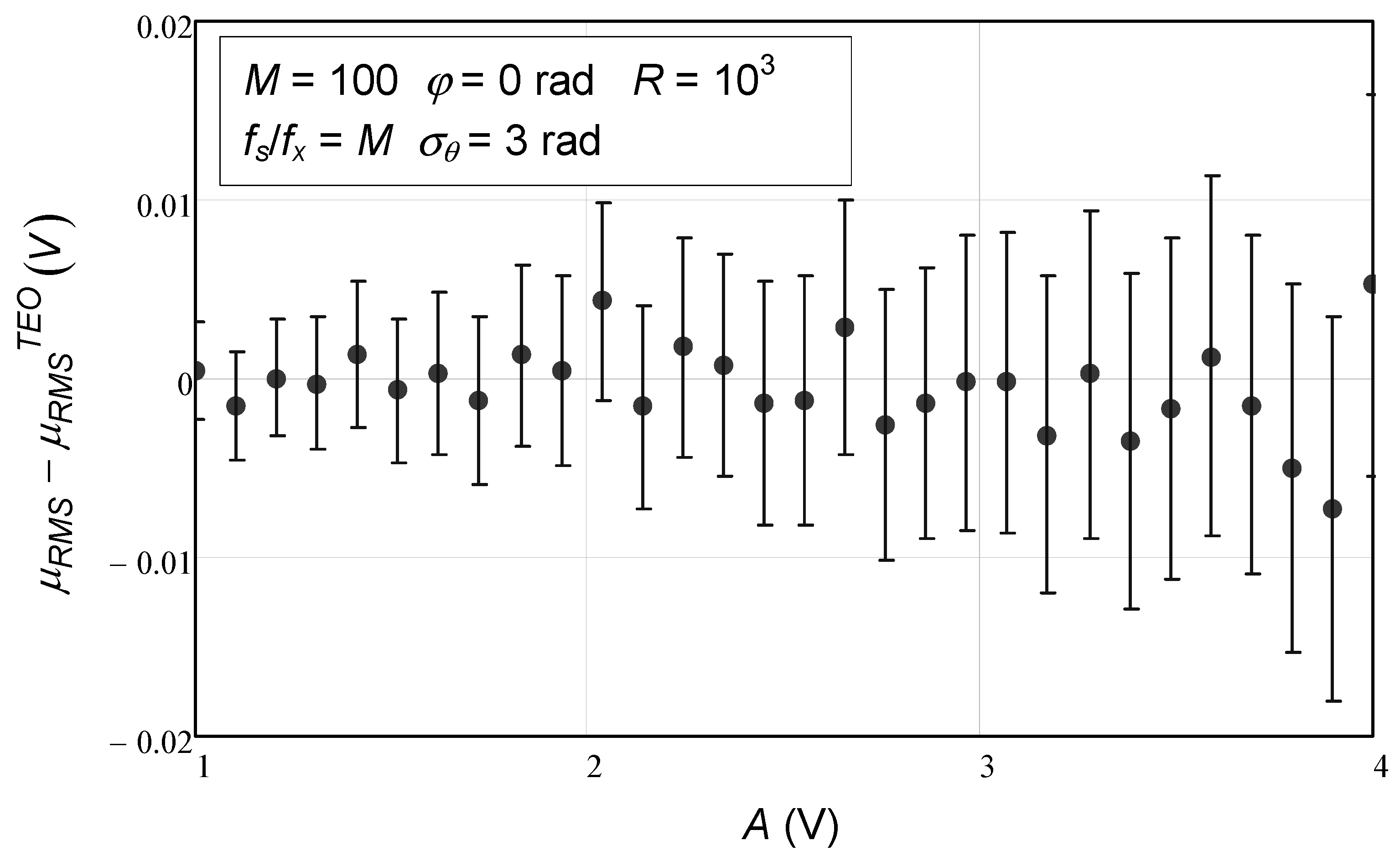
At this point in the presentation, the two derived analytical expressions will be put to the test by numerically simulating a set of data points that are corrupted by phase noise, fitting them to the sinusoidal model described above, determining the resultant residuals, and computing their root mean square value. Three parameters are going to be varied in this study, namely the injected phase noise standard deviation, the number of data points, and the sinusoidal amplitude, all of which are parameters that these two analytical expressions depend on. In general, for each case, we will present the average and the standard deviation of the RMS estimation, together with the values given by the analytical expressions derived here. The numerically obtained values are presented in a graphical form using error bars, which correspond to a confidence interval computed for the confidence level of 99.9%. The values obtained with the analytical expressions will be plotted in the same charts using a solid line. The goal is to have all the error bars located around the solid lines. As we will see, this happens in almost all instances, showcasing the range of validity of the analytical expressions derived. A second set of charts will present the difference between the numerical simulation values and the ones given by the analytical expressions derived here.

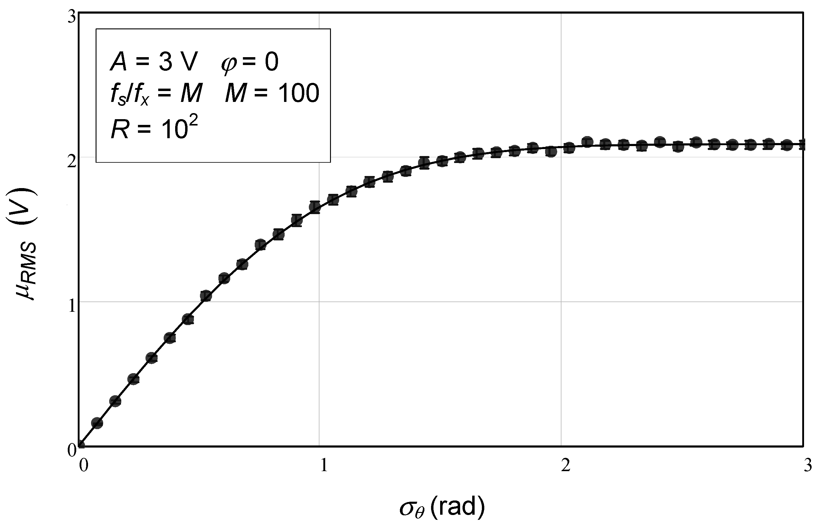
The first study presented here concerns the use of different amounts of injected phase noise. In Figure 1, we observe the mean values of RMS estimation as a function of phase noise standard deviation over a range up to 3 rad. In this instance, the error bars are so short that they are practically invisible. In any case, the circles representing the middle point of the error bars follow closely the values given by the analytical expression. In this example, a sinusoidal amplitude of 3 V and 100 samples (M) was used. Note that the number of simulation repetitions used to compute the error bars (R) was, in this case, 100. The more repetitions are used, the shorter the error bars become, but the longer the numerical simulation takes.

In this figure, we confirm the complete agreement between the numerical simulations and the theoretical expression (116). Furthermore, in Figure 2, we plot the difference between the values from numerical simulation and the ones from the analytical expression. Once again, a complete agreement is observed, since in this instance all error bars are around 0, which shows that the analytical expression indeed accurately reproduces the relationship between the phase noise or jitter phase noise standard deviation and the expected value of the estimated RMS value of the residuals.

In

Table 1. Data points for the mean RMS for different values of phase noise standard deviation in the case of a sinusoidal amplitude of 3 V, initial phase null, and 100 data points. The number of repetitions is 100.

Phase Noise Standard Deviation (rad)	Theoretical Value (V)	Error Bar Minimum (V)	Error Bar Maximum (V)	Simulation Value (V)
1	1.626	1.615	1.693	1.654
2	2.071	2.037	2.090	2.063
3	2.090	2.057	2.114	2.086

, one can see the theoretical and numerical mean values of RMS for some of the phase noise standard deviation cases.

The range of values tried in the numerical simulation is far greater than the ones shown here; however, since no substantive difference in conclusions is warranted, and for the sake of conciseness, we choose to present just a few illustrative cases.

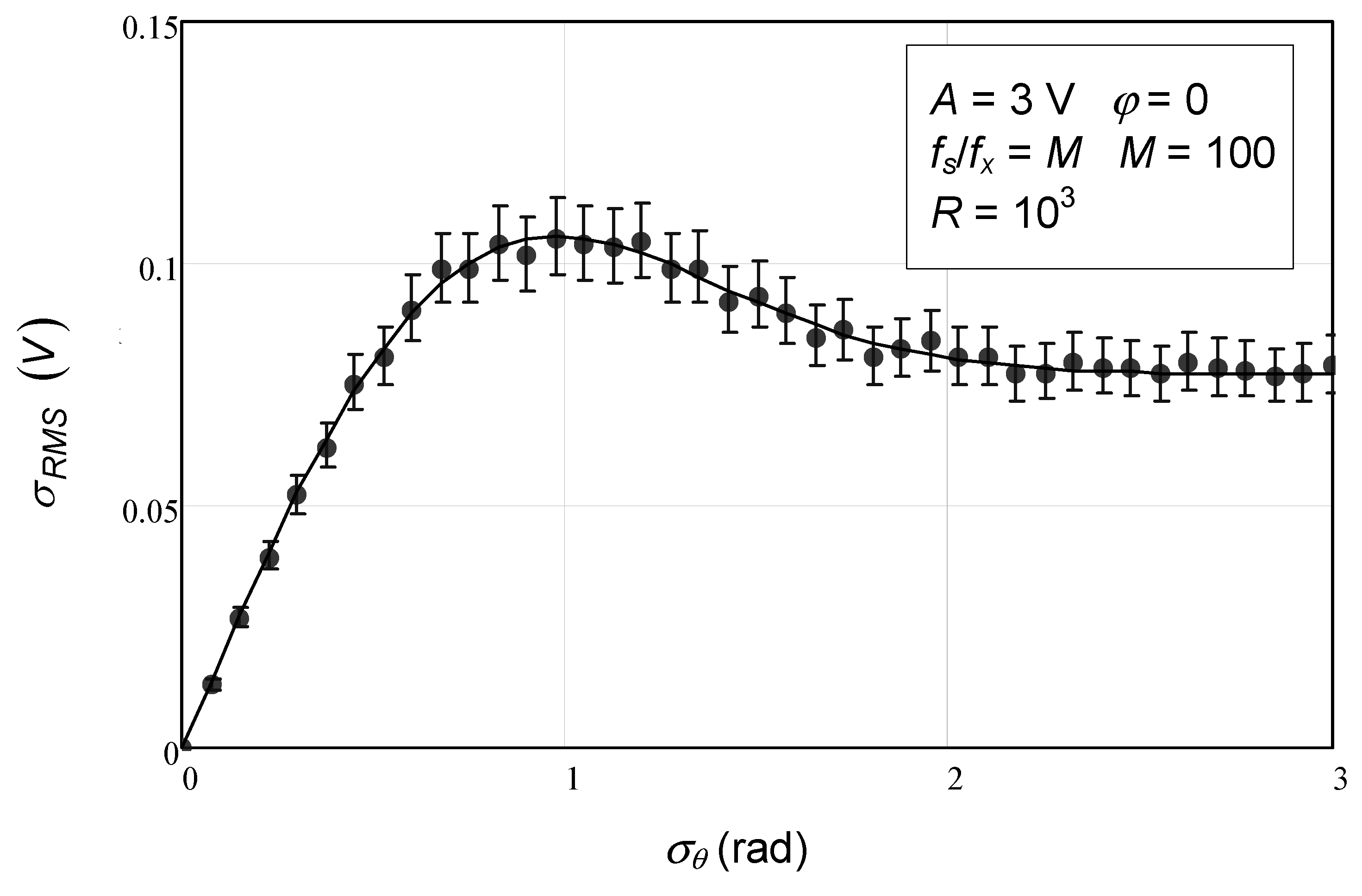
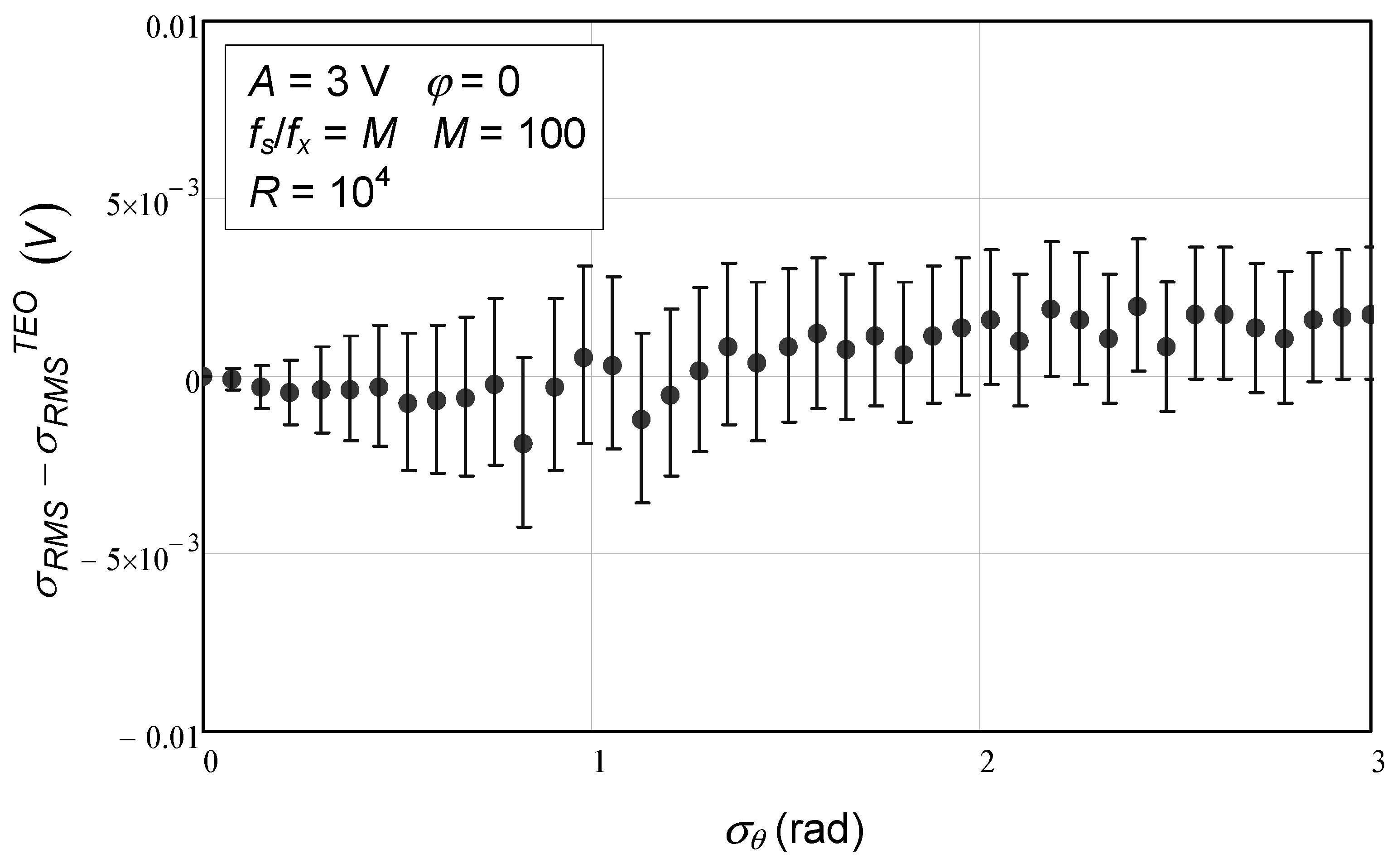
In Figure 3 and Figure 4, we observe the equivalent results for the estimated RMS standard deviation. In this case, the theoretical expression is the one presented in (120). Again, complete agreement is found. In Figure 3, one can observe the theoretical expression depicted with the solid line and the error bars from the numerical simulations made with 1000 repetitions.

In Figure 4, one can see the difference between the analytical expression and the numerical simulation results. The error bars are very close to 0, which means that the approximated analytical expression for the standard deviation of the RMS value of the residuals provides an excellent approximation, albeit not exact, due to the use of a Taylor series approximation with just one term.

In

Table 2. Data points for the standard deviation of RMS estimation for different values of phase noise standard deviation in the case of a sinusoidal amplitude of 3 V, initial phase null, and 100 data points. The number of repetitions is 100.

Phase Noise Standard Deviation (rad)	Theoretical Value (V)	Error Bar Minimum (V)	Error Bar Maximum (V)	Simulation Value (V)
1	0.106	0.098	0.114	0.105
2	0.080	0.075	0.087	0.081
3	0.077	0.073	0.085	0.079

, one can see the theoretical and numerical standard deviation values of RMS estimation for some of the phase noise standard deviation cases.

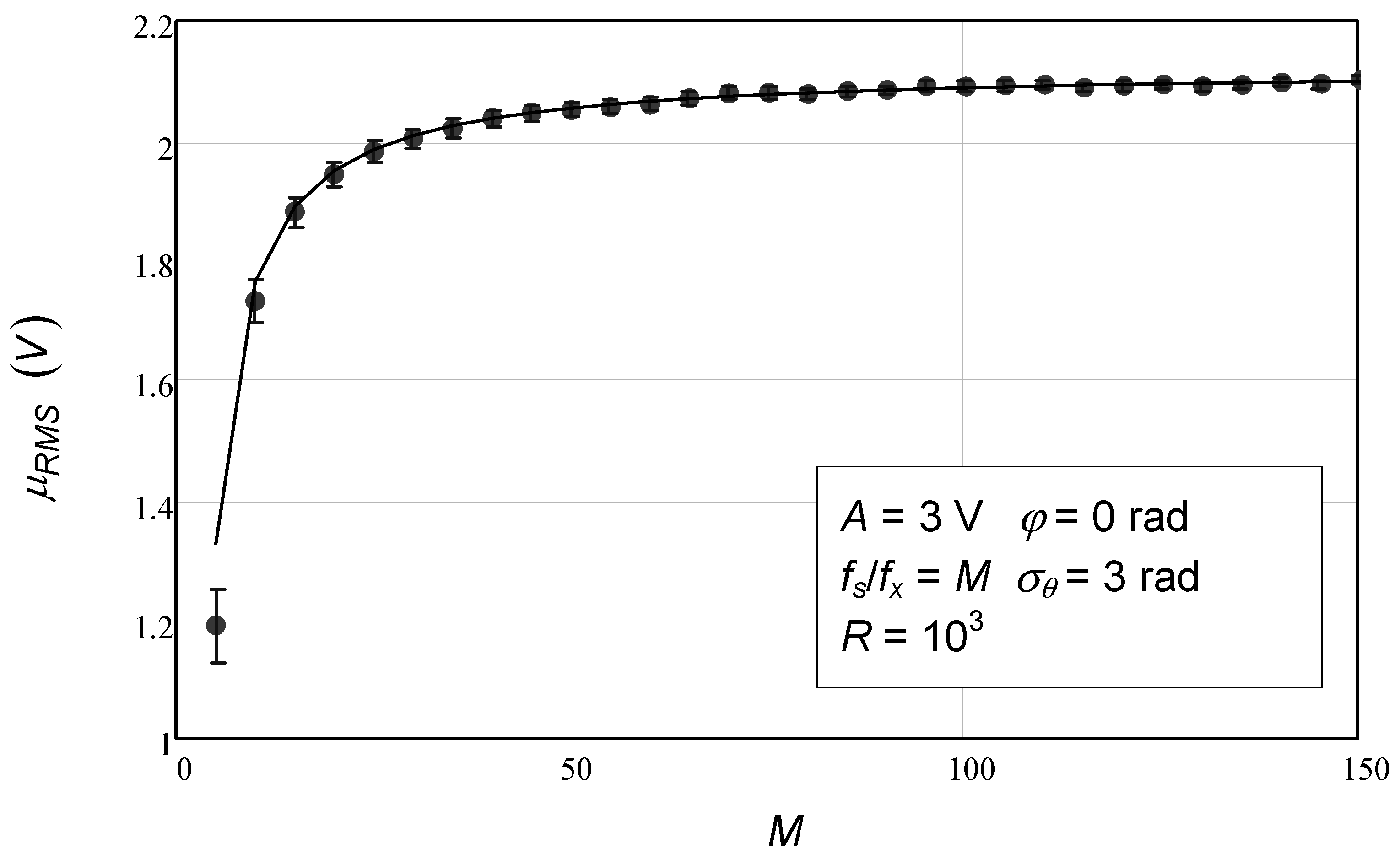
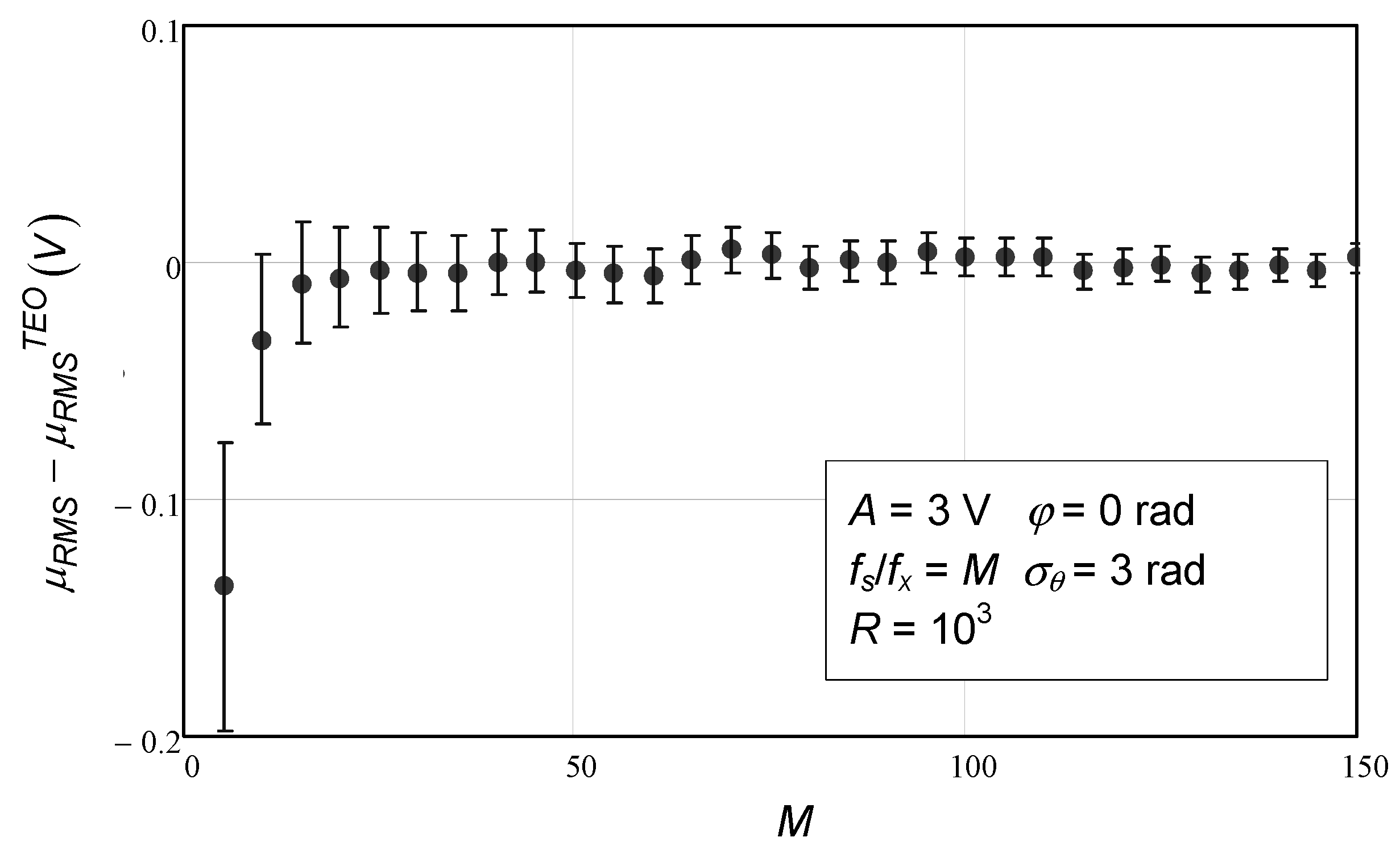
In the next set of charts, the number of samples was varied from 5 to 150, and the phase noise standard deviation was kept constant at 3 rad. Other values were also used, but the conclusions are the same, and so we refrain from showing them here. Figure 5 shows the mean value of the RMS value estimation as a function of the number of samples. The agreement between numerical simulation values and the analytical expression (solid line) is strong, except when the number of data points is very low (5). Recall that some approximations were performed during the theoretical derivation in order to obtain analytical expressions that were as simple as possible but still fairly accurate.

Figure 6 shows the difference between numerical simulation values and the ones provided by the analytical expression for varying numbers of data points. Again, we see that for a very small number of data points, the difference is not negligible.

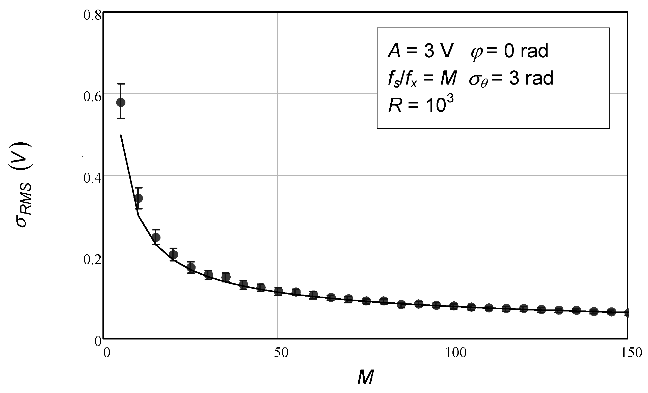
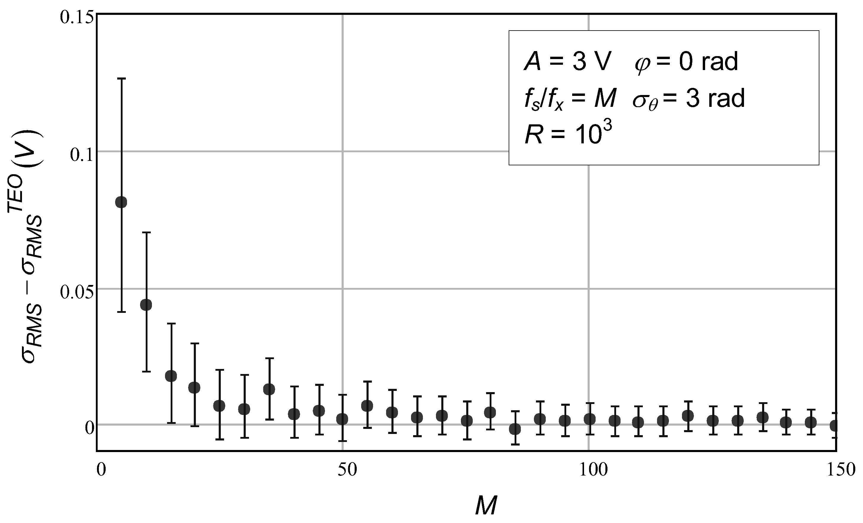
In Figure 7 and Figure 8, we see the behavior of the standard deviation of the RMS value estimation as a function of the number of data points. Again, strong agreement is found, except for the first data points that correspond to a very low number of samples. In Figure 7, we see the standard deviation of the RMS value of the residuals as a function of the number of data points. The solid line, corresponding to the theoretical expression, lies around the error bars, which in some cases (large number of samples) are so small that they become invisible, and only the middle point (circles) can be observed. The exception is in the first four data points.

In Figure 8, we observe the difference between numerical simulation values and theoretical ones. Here, we can observe more clearly the discrepancy in the first four data points. As expected, the smaller the number of data points, the worse the Taylor series approximation. One could have used more terms of the Taylor series to achieve a better agreement, but that would lead to a more complex and cumbersome analytical expression.

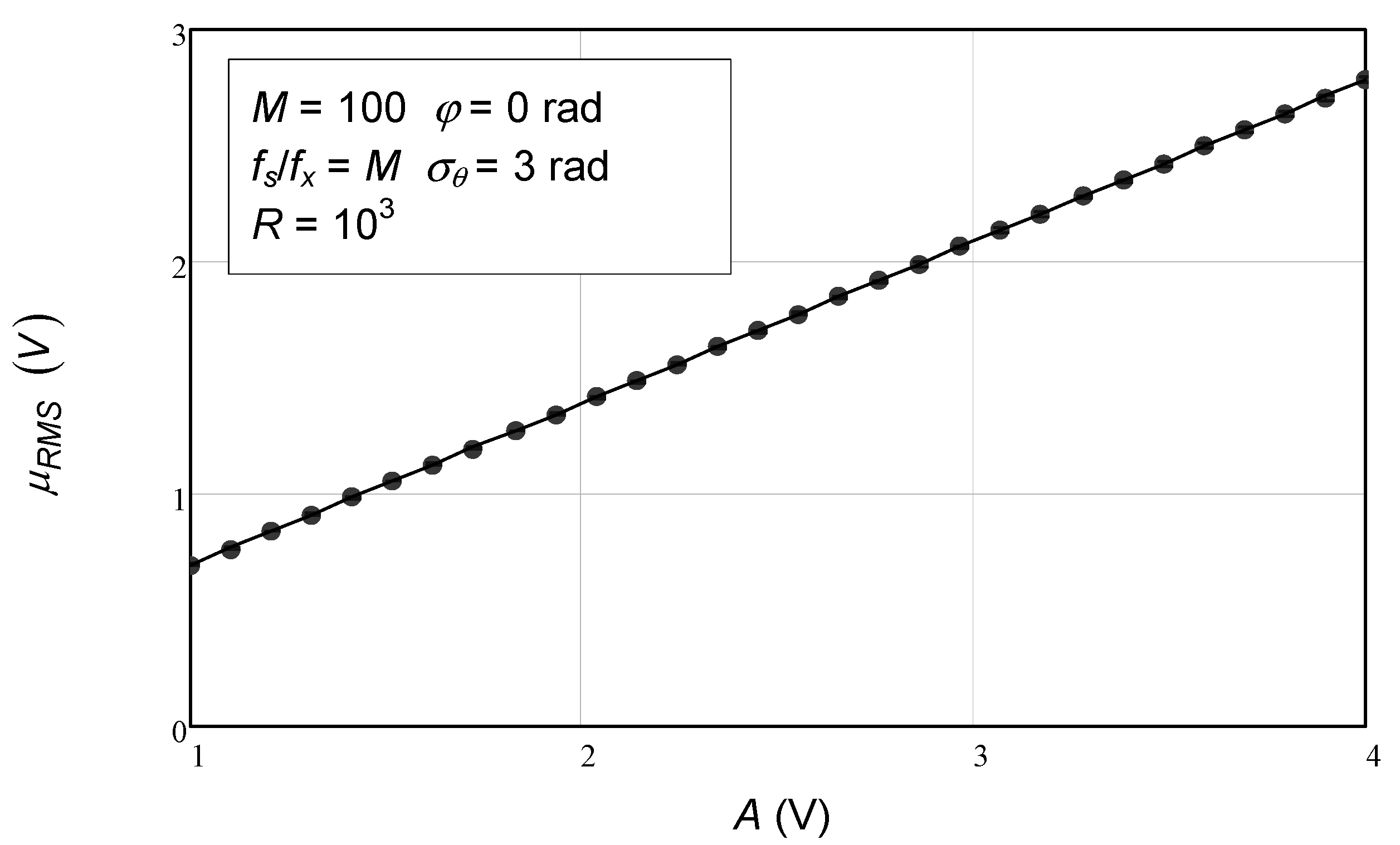
The final set of numerical simulation results pertains to varying sinusoidal amplitude. In Figure 9, we observe the linear behavior provided by the analytical expression for the dependence of the mean value of the estimated residual RMS as a function of sinusoidal amplitude, as expressed by Equation (116). Again, for the number of repetitions used, R = 1000, the error bars for the numerical simulation results are invisible, and only the middle points (circles) are visible. As observed, all the circles are on top of the solid line. Note that this simulation was made for 100 samples. As mentioned before, if the number of samples is less than 10, the agreement deteriorates significantly.

In Figure 10, we see more clearly that the numerical simulation values and the analytical expression agree for different values of sinusoidal amplitude, since all the error bars are located around 0 for this specific case, where 100 (M) samples were used.

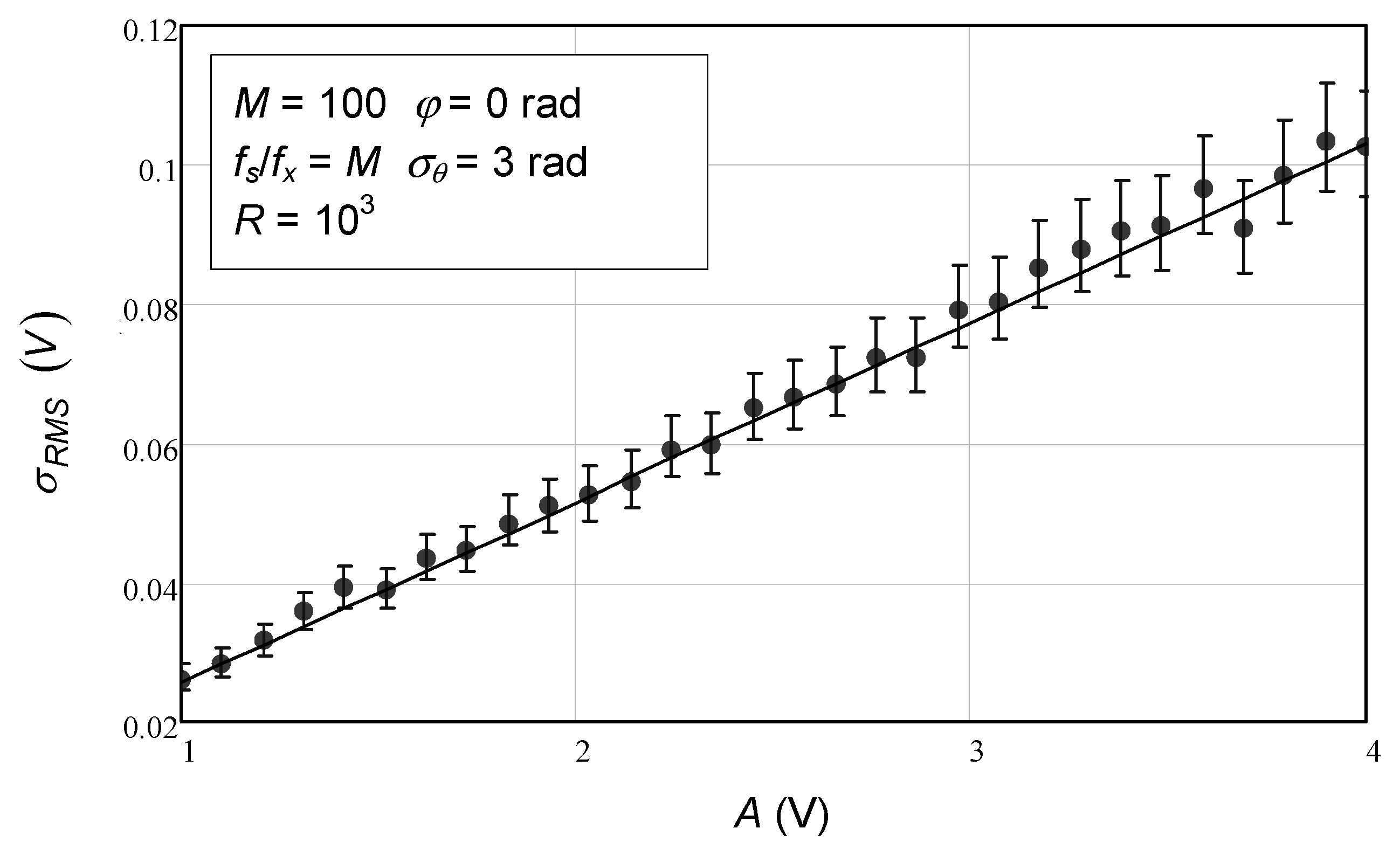
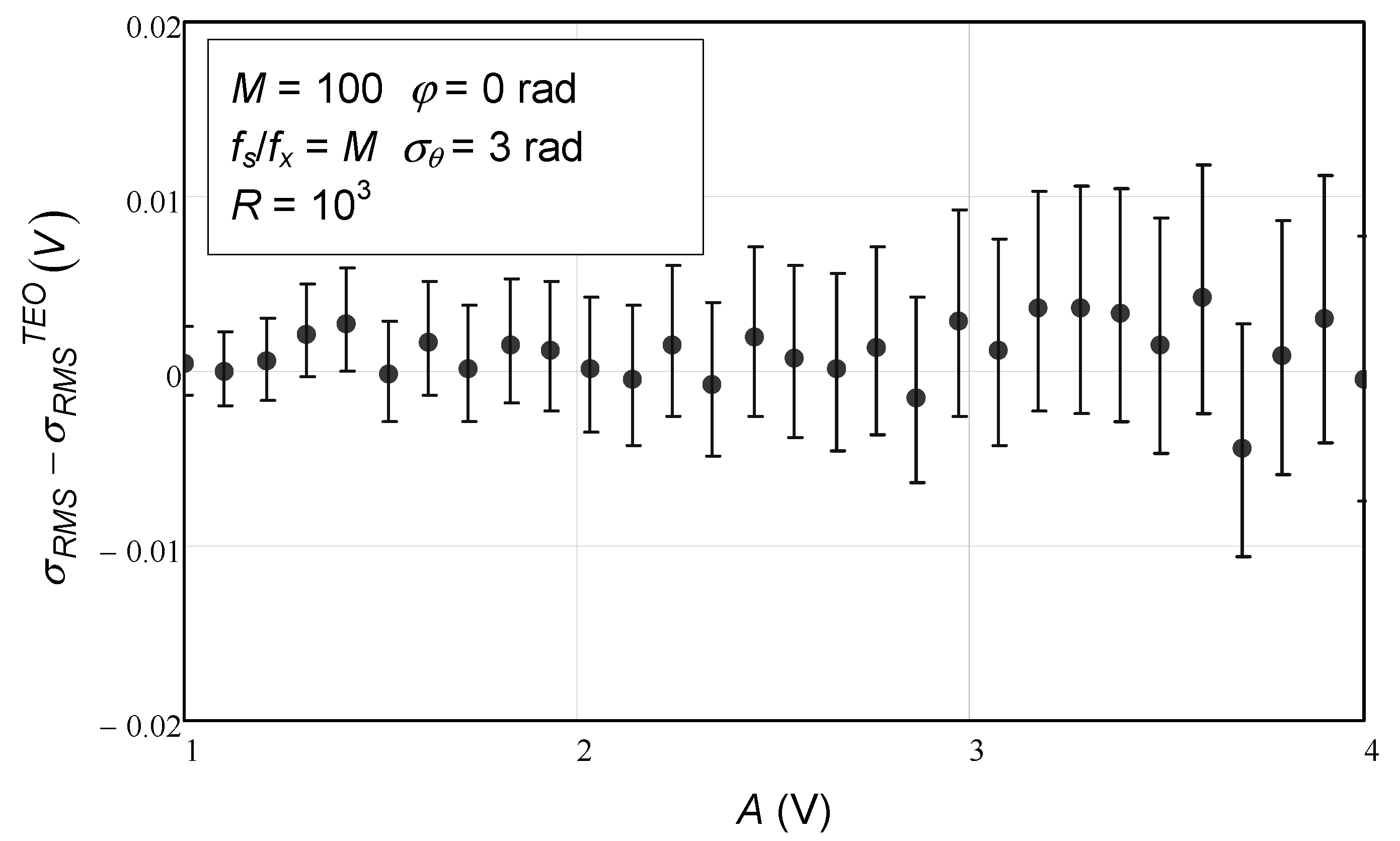
In Figure 11 and Figure 12, we see the last set of results that pertain to the RMS estimation standard deviation as a function of the sinusoidal amplitude. Again, the agreement with the theoretical expression derived here and presented in Equation (120) is strong. In Figure 11, all the vertical bars corresponding to the numerical simulation results are on top of the solid line representing the analytical expression.

In Figure 12, the difference between the theoretical values and those from the numerical simulations is more clearly seen. As expected, the error bars are all around 0.

The numerical simulation results presented in this section completely validate the analytical derivations presented in this work. This provides assurance to the engineer that the two analytical expressions obtained (for the mean and for the standard deviation of RMS value estimation) can be used with confidence.

7. Conclusions

This paper has developed a strong theoretical framework to understand and quantify the influence of phase noise and sampling jitter on sinusoidal fitting residuals, fundamentally contributing to the measurement science literature. The rigorous derivation of closed-form analytical expressions for the mean and variance of the root mean square (RMS) estimation of sine-fitting residuals is a sustainable contribution to the measurement science literature and furthers the knowledge of measurement uncertainty when considering either generator phase noise or sampling jitter. The detailed numerical validation through Monte Carlo simulations provides considerable confidence that the derived expressions accurately represent the actual behavior of residuals and will reflect reasonably strong estimates for very diverse operating conditions. Excellent agreement with the analytical predictions when compared to simulations, which were shown for varying amounts of phase noise, different numbers of data points, and different signal amplitudes, clearly illustrates that the developed theory will have wide applicability for real-world measurement purposes. Additionally, throughout the validation, it was confirmed that the assumptions and approximations made during the analytical derivation were reasonable for the intended domain of application. Developing theoretical knowledge of this structure is considered a significant development in the field of measurement uncertainty; however, it is an important consideration to discuss the potential limits and assumptions that will limit its domain of application.

In the future, the results presented here can be used as a starting point to study the uncertainty of other estimators that are based on sine-fitting residuals, like signal-to-noise ratio, noise floor, or effective number of bits, for example.

As a final comment, the author wants to reiterate that the knowledge of the standard deviation value of an estimator is important for an engineer who, when performing a measurement or numerical estimation of some kind where random phenomena are at play, must always specify the confidence intervals for their estimates.