Earthquake Precursors Based on Rock Acoustic Emission and Deep Learning

Abstract

China is one of the countries severely affected by earthquakes, making precise and timely identification of earthquake precursors essential for reducing casualties and property damage. A novel method is proposed that combines a rock acoustic emission (AE) detection technique with deep learning methods to facilitate real-time monitoring and advance earthquake precursor detection. The AE equipment and seismometers were installed in a granite tunnel 150 m deep in the mountains of eastern Guangdong, China, allowing for the collection of experimental data on the correlation between rock AE and seismic activity. The deep learning model uses features from rock AE time series, including AE events, rate, frequency, and amplitude, as inputs, and estimates the likelihood of seismic events as the output. Precursor features are extracted to create the AE and seismic dataset, and three deep learning models are trained using neural networks, with validation and testing. The results show that after 1000 training cycles, the deep learning model achieves an accuracy of 98.7% on the validation set. On the test set, it reaches a recognition accuracy of 97.6%, with a recall rate of 99.6% and an F₁ score of 0.975. Additionally, it successfully identified the two biggest seismic events during the monitoring period, confirming its effectiveness in practical applications. Compared to traditional analysis methods, the deep learning model can automatically process and analyse recorded massive AE data, enabling real-time monitoring of seismic events and timely earthquake warning in the future. This study serves as a valuable reference for earthquake disaster prevention and intelligent early warning.

1. Introduction

Earthquakes are a natural phenomenon that releases energy from the Earth’s interior, resulting in significant destruction and devastating consequences for human society. China, situated at the intersection of the Pacific Rim Seismic Zone and the Eurasian Seismic Zone, is one of the countries most severely affected by seismic disasters. Conducting scientific research on earthquake precursors and exploring methods for identifying earthquake precursors are crucial for disaster prevention and mitigation. Currently, earthquake precursor identification primarily relies on the observation and analysis of various precursors, including crustal deformation, changes in seismic wave velocity, and geomagnetic field anomalies. Researchers have examined a range of precursor anomalies before earthquakes and have sought to identify seismic events based on the precursor information. Among the studies, Chien et al. [1] investigated the relationship between geothermal precursor anomalies and the locations of future earthquakes in Taiwan Island, Singh et al. [2] analysed the correlation between hydrogen peroxide concentrations in hot spring boreholes and earthquakes in active fault zones, Li et al. [3] developed a short-term earthquake warning technique based on continuous GPS signal anomalies, and Yusof et al. [4] sought to identify earthquake precursor features and verify their correlation with seismic events through signal processing methods. However, these precursor signals often exhibit significant uncertainties in complex geological environments, which can limit the accuracy and timeliness of precursor identification. Consequently, exploring new earthquake precursor signals and their identification methods has become crucial for effective earthquake early warning.

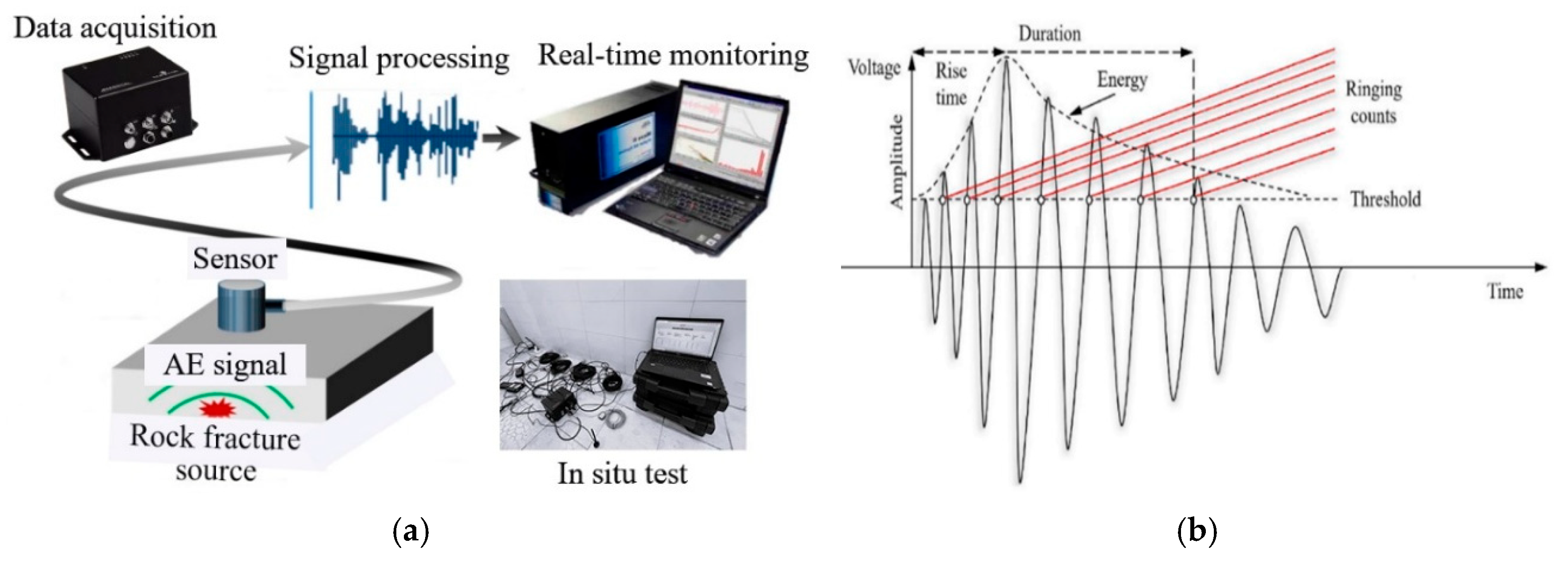
Rock acoustic emission (AE) monitoring techniques based on fracture mechanics are cutting-edge tools for geophysical diagnostics. During the earthquake preparation phase, a large area of crustal rock is subjected to compression, leading to the accumulation of significant strain energy. In regions of high compression before an earthquake, localised fractures in the rock can occur, resulting in concentrated and intense AE phenomena. In fracture mechanics, AE represents the strain energy released during material fracture, which is emitted as stress waves [5,6,7]. These stress waves exhibit a wide frequency range, from 1 THz for nanoscale fractures to 1 Hz for kilometre-scale fractures. The latter frequencies correspond to typical seismic wave frequencies, which can be detected by sensors placed on the earth’s surface [8]. Therefore, by monitoring the rock AE, it is possible to detect AE signals generated by micro-seismic activities before an earthquake, allowing for early earthquake warning. This method has been studied in laboratory settings [9], but it is rarely measured in the field. Research has indicated that crustal stress changes during the earthquake preparation phase [10], and an increase in AE activity may signify the redistribution of crustal stress in the preparation zone [11,12]. Zimatore et al. [13] analysed AE time series obtained from two monitoring stations located 300 km apart in Italy and found that AE can provide information about crustal stress anomalies related to earthquakes. Studies examining the correlation between AE and seismicity suggest that AE can serve as an earthquake precursor [14,15]. For instance, a sudden and significant increase in AE signals was observed at about 400 km of distance from the epicentral area before the occurrence of the Assisi earthquake [16]. Carpinteri et al. [17] identified a strong correlation between AE and seismic sequences in adjacent areas through experimental observations in gypsum mines in northern Italy, Lukovenkova et al. [18] noted a distinct difference in the frequency domain of pre-seismic AE signals compared to the usual background signals during the Chupanov earthquake, and Spivak et al. [19] studied the propagation and perturbation of AE signals in the atmosphere related to earthquakes of magnitudes 5.1 to 6.9 in Albania, Greece, Iran, and Turkey, estimating the energy of these earthquakes based on spectral features. These studies illustrate that AE monitoring techniques offer a viable approach for short-term earthquake warning.

However, during AE monitoring, the data acquisition systems record massive data that include noise from multiple sources, making it challenging to identify useful information in real time through manual analysis. With the rapid advancement of artificial intelligence [20,21], the incorporation of deep learning holds the potential to significantly enhance technological progress in the field of earthquake precursor identification. Deep learning technology provides robust data processing and recognition capabilities, enabling the automatic analysis of large volumes of AE data to reveal inherent earthquake precursor features. In recent years, many scholars have explored deep learning methods for earthquake warning [22,23,24,25]. Banna et al. [26] developed a long short-term memory (LSTM) model for identifying seismic events in Bangladesh within a month, whereas Jozinovi et al. [27] utilised a convolutional neural network (CNN) to identify distant peak ground intensity. Additionally, researchers developed CNN-LSTM models for identifying significant earthquakes in Japan [28], daily seismic events in Chile [29], seismic acoustic signals from lab simulations [30], and coal mine earthquakes [31]. While these studies demonstrate impressive advancements in earthquake warning, they also exhibit certain limitations. For instance, many models, including those by Wang et al. [32], might be constrained by their reliance on specific geographic data and may not generalise well to different regions. Shcherbakov et al. [33] combined Bayesian networks with extreme value theory; although innovative, this approach may overlook certain real-time data integration challenges. Furthermore, the use of deep learning by DeVries et al. [34] on over 130,000 main and aftershock pairs could be constrained by the quality and range of input data, potentially impacting warning accuracy. These shortcomings present critical gaps that this paper aims to address, and real-time forecasting requires the timely processing of massive amounts of data. By improving real-time data integration, enhancing model adaptability, and refining input data quality, we aspire to advance the state of deep learning applications in earthquake precursor identification.

Existing research has not yet produced a comprehensive model that fully addresses the challenges of earthquake precursor identification, primarily due to the complex physical mechanisms that generate earthquakes and their precursors. However, with the continuous advancement of AE monitoring technology and deep learning, it is essential to conduct in-depth studies on earthquake precursor identification. Rocks in the deeper layers of the Earth’s crust typically reflect stress changes more directly, and the signal attenuation of stress wave propagation in rocks is relatively slow, making them more sensitive to micro-seismic activities. Therefore, monitoring AE signals in rocks allows for the acquisition of more accurate information about earthquake precursors while minimising noise interference.

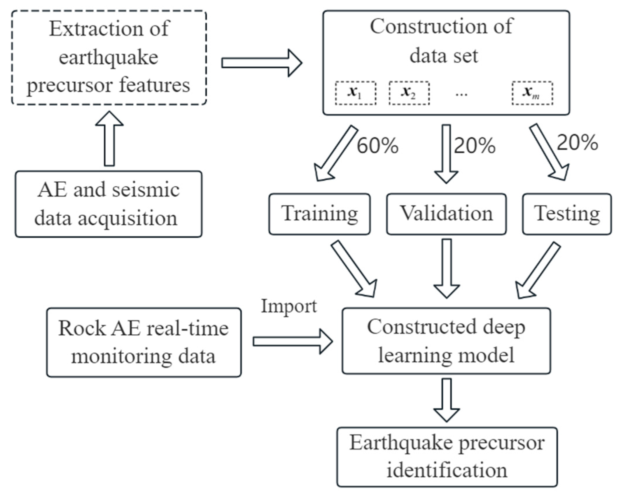
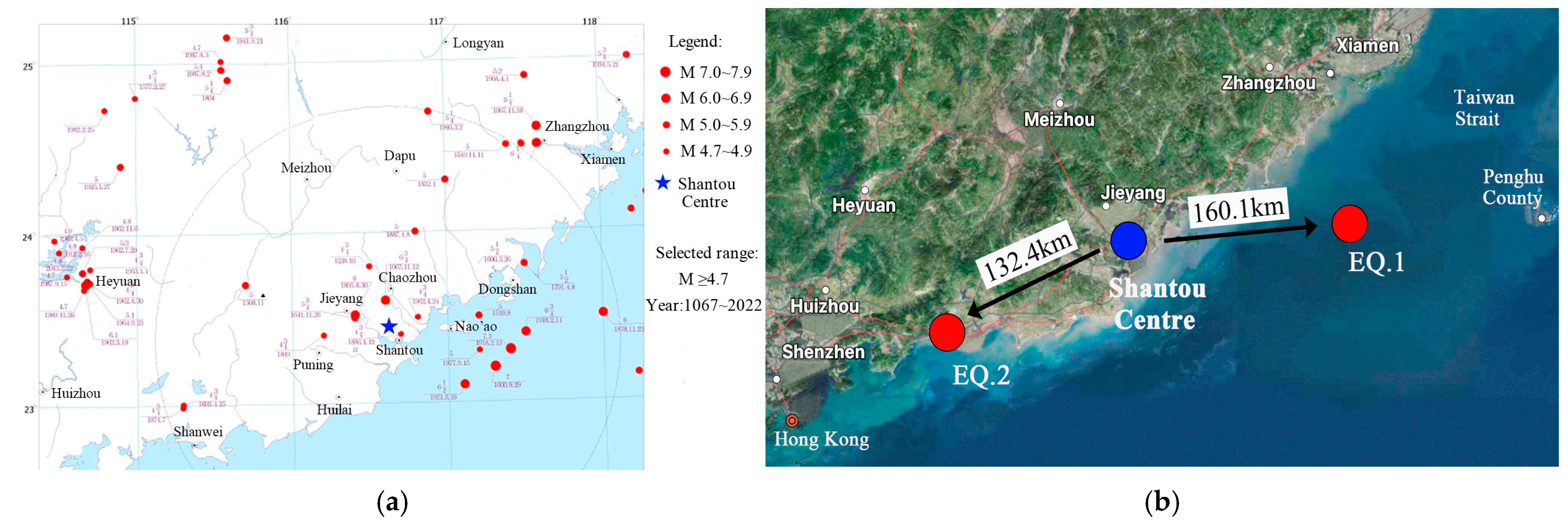
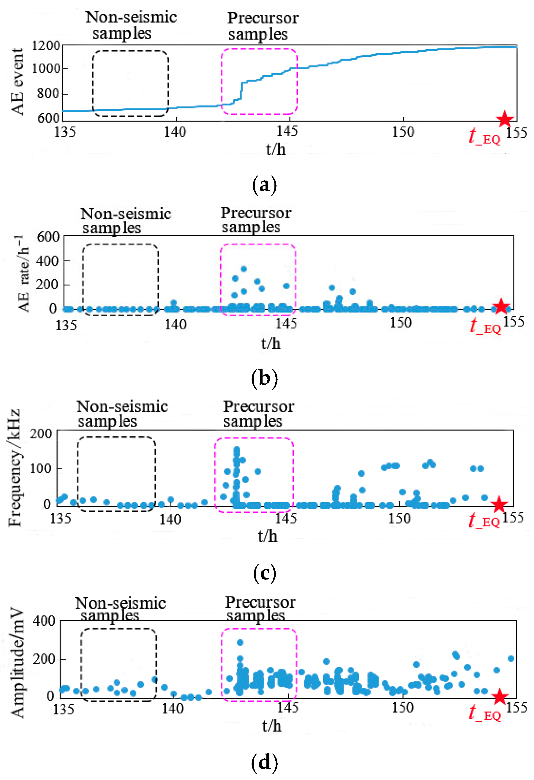
The eastern Guangdong region of China is located within the Southeast Coastal Seismic Zone and the Pacific Rim Seismic Zone, and is recognised as a high-seismic-intensity zone. This paper utilises a dedicated seismic observation station in eastern Guangdong to investigate a rapid earthquake precursor identification method through AE and deep learning. In this study, AE equipment and seismometers are installed in a dedicated all-granite mountain tunnel to collect AE signals and seismic activity from the rocks in the high-intensity zone. The process involves extracting samples containing precursor features, which are then combined with deep learning models for training, validation, and testing. The resulting warning model is designed for rapid earthquake warning. This study offers a new technical approach to earthquake precursor identification that may help to prevent earthquake disasters in the future.

2. Deep Learning-Based Identification of Earthquake Events

2.1. Overview of Identification Workflow

Based on real-time monitoring data of rock AE in mountain tunnels, this paper proposes a novel method for identifying precursors of seismic events utilising AE time-series features and deep learning. The workflow is illustrated in Figure 1, where [x₁], [x₂], …, [x_m] represents the extracted AE time-series features containing earthquake events.

The approach is outlined as follows: first, AE signals from the rocks are recorded, followed by the extraction of features and analysis of the changes in the time-series signals. Next, the extracted AE features of earthquake precursors are used as inputs to train a deep learning model for the classification and identification of seismic events. Finally, this model is ultimately employed for binary classification, distinguishing between the presence and absence of earthquakes, following model training and parameter optimisation.

2.2. Deep Learning Model

The deep neural network is a multilayer feed forward network that consists of an input layer, hidden layers, and an output layer. Hidden layers may consist of multiple layers, each containing neurons interconnected with adjacent layers. The connections between the layers are governed by weights (w) and biases (b), as illustrated in Figure 2. The network initialises w and b randomly and applies an activation function to compute the predicted output ($\widehat{y}$). These parameters are iteratively updated via back propagation, minimising the loss between predicted and true values to an acceptable level. Deep neural networks effectively capture complex nonlinear relationships, enabling automated analysis of large AE datasets to extract precursor features [35,36].

The fundamental unit of the neural network is the neuron, which mimics the behaviour of biological brain neurons by linearly combining inputs and computing its output (y) as defined by Equation (1):

$$y=\sigma (\sum w_i{x}_i+b)$$

(1)

where x_i and w_i represent the individual inputs to the neuron and their corresponding weights (see Figure 2), b denotes the bias, and σ(x) is the activation function, which may include options such as the Sigmoid function defined in Figure 2:

$$\sigma (x)={\displaystyle \frac{1}{1+e^{-x}}}$$

(2)

The algorithmic model in this study is implemented using Python 3.9, with the Pytorch 2.3.1 deep learning framework for constructing and training. The experiments are conducted on a Windows operating system, leveraging an AMD Ryzen processor and an Nvidia RTX 8000 GPU for acceleration.

The training process consists of forward calculation, back propagation, and weight updating. A single pass through the entire training set is called an epoch, during which the loss function is evaluated on the validation set as a metric for performance. The loss function utilises the binary cross-entropy (BCELoss) function (see Equation (3)), where y_n represents the output values of the training samples and ${\widehat{y}}_n$ denotes the network’s predicted values, as indicated in Equation (3). The updated w is calculated according to Equation (4).

$$loss=-{\displaystyle \frac{1}{N}}\sum _{n=1}^N y_{n}log{\widehat{y}}_n+(1-y_n)log(1-{\widehat{y}}_n)$$

(3)

$$w=w-\alpha {\displaystyle \frac{\mathsf{\partial }loss}{\mathsf{\partial }w}}$$

(4)

As shown in Figure 2, the input layer consists of the extracted AE features (x₁, x₂, x₃, x₄), such as AE event, AE rate, frequency, and amplitude, respectively. The output layer (y) produces two types of outcomes: one indicating the presence of the earthquake (label 1) and the other indicating the absence of the earthquake (label 0). Therefore, the training model can be regarded as a multi-dimensional binary classification problem, implemented using the Pytorch framework for binary classification tasks.

2.3. Training of Deep Learning Models

Using the extracted AE features as input, a deep learning algorithm is employed to develop a binary classification model for real-time monitoring and identification of seismic events. The dataset containing precursor features is divided into a training set (60%), a validation set (20%), and a test set (20%), following the ratio of 3:1:1, as summarised in

Table 1. Dataset division and number distribution.

Types	Training Set	Validation Set	Test Set
Precursor samples	1368	456	456
Non-seismic samples	1368	456	456
Total	2736	912	912

. Balanced training of the samples is achieved by maintaining the ratio of extracted precursor samples (Label 1) to non-seismic samples (Label 0) at approximately 1:1. The training process for the identification model is illustrated in Figure 3.

2.4. Metrics for Evaluating Model Performance

The output of deep learning models is typically framed as a binary classification problem, with evaluation metrics including accuracy, precision, and recall [37]. Considering the occurrence of earthquakes as positive samples and their absence as negative samples, the test results can be classified into four categories: True Positive (T_P), True Negative (T_N), False Positive (F_P), and False Negative (F_N), as illustrated in

Table 2. Overview of the confusion matrix.

Actual Value	Predicted Value
	1	0
1	TP	FN
0	FP	TN

. Specifically, T_P and T_N represent the counts of correctly predicted positive and negative samples, respectively, whereas F_P and F_N denote the counts of incorrectly predicted positive and negative samples. Accuracy (A_cc) is a key evaluation index, which is calculated using the equation presented in Equation (5) and represents the proportion of correctly predicted samples to the total number of samples, indicating that higher accuracy reflects better model performance.

$$A_{cc}={\displaystyle \frac{T_p+T_N}{T_p+T_N+F_P+F_N}}$$

(5)

The F₁ score, a composite metric, is the harmonic mean of Precision (P_r) and Recall (R_e), providing a more comprehensive evaluation of model performance, as calculated in Equation (6).

$$F_1={\displaystyle \frac{2P_r{R}_e}{P_r+R_e}}$$

(6)

Here, P_r represents the proportion of correct predictions among all positive predictions, as calculated in Equation (7). In contrast, R_e indicates the proportion of correct predictions among all actual positive samples, making it particularly relevant to assess actual performance, as calculated in Equation (8).

$$P_r={\displaystyle \frac{T_P}{T_P+F_P}}$$

(7)

$$R_e={\displaystyle \frac{T_P}{T_P+F_N}}$$

(8)

3. Construction of AE and Seismic Dataset

3.1. In Situ Monitoring of Mountain Tunnel

The test was carried out inside the Shantou Seismic Monitoring Centre, located in eastern Guangdong at a latitude of 23.41° N and a longitude of 116.63° E. The location of the monitoring centre is illustrated in Figure 4. The dedicated tunnel is an all-granite inner tunnel, horizontally excavated to a depth of up to 150 m, used for installing seismic observation instruments. Since the monitoring centre is located within this dedicated tunnel, environmental disturbances impacting AE monitoring, such as ambient traffic, human activities, and wind effects, have been significantly reduced [38].

To capture signal features associated with earthquakes, the AE system used in this study incorporates a specialised seismic monitoring device, ÆMISSION^®, manufactured by Lunitek, Italy. This acquisition system is equipped with eight piezoelectric sensors that operate within a frequency range of 10 to 10³ kHz. As shown in Figure 5, the AE sensors were affixed to the floor of the specialised tunnel, and a seismometer was also installed to monitor seismic activity over a continuous period of approximately 35 days.

3.2. Analysis of Seismic Monitoring Results

The Pacific Rim Seismic Zone accounts for about 80% of global earthquakes, including over 80% of shallow quakes, 90% of moderate-depth quakes, and nearly all deep-source quakes. The southeastern coast of China, particularly the Taiwan Strait, lies within the Pacific Rim Seismic Zone. Shantou’s seismic design intensity is VIII, placing it in a strong earthquake zone [38]. The most significant recorded earthquake in Shantou’s history was the 7.3 magnitude quake on Nan’ao Island in 1918. Historical seismic activity in the region is shown in Figure 6a. Between 1067 and 2022, 51 earthquakes with magnitudes of M ≥ 4.7 were recorded, highlighting high regional seismic activity.

During the monitoring period, two relatively strong earthquakes were recorded: the Taiwan Strait earthquake (magnitude 3.2, EQ.1) and the Guangdong Hai Feng Sea earthquake (magnitude 2.4, EQ.2). The epicentre of EQ.1 was at 23.37° N, 118.57° E, while EQ.2 was located at 22.83° N, 115.24° E, as shown in Figure 6b. The AE monitoring system detected precursors for earthquakes occurring at distances of 100~200 km from the tunnel. Epicentral distances were derived from geographic coordinates, while hypocentral depths were not explicitly measured in this study. While the two seismic events in our study were relatively small, they served as valuable preliminary cases to validate the correlation between AE patterns and seismic precursors, laying the groundwork for future research on larger earthquakes.

This paper employs a multi-peak statistical analysis method to process seismic data. Peak locations are identified from data distribution curves and evaluated using Gaussian fitting to obtain the best-fit distribution curves.

As shown in Figure 7a, the Gaussian distribution that best approximates the discrete distribution of the original seismic data is determined through iterative adjustments of parameters such as offset (y₀), centre (x_c), width (w), and amplitude (A). Based on the temporal distribution of the 24 earthquakes recorded during the 35-day monitoring period, two primary earthquake clusters are clearly identified, as depicted in Figure 7b. The Gaussian distribution function is expressed as follows:

$$y=y_0+A{e}^{(-e^{-z}-z+1)}$$

(9)

$$z={\displaystyle \frac{x-x_c}{w}}$$

(10)

3.3. AE Time-Series Identification Method

The fundamental principle of AE detection is illustrated in Figure 8a. Monitoring changes in rock AE signals enables the detection of stress waves from micro-seismic activities before earthquakes occur, with AE sensors capturing these waves as precursor signals. The AE sensors convert the stress signals into electrical signals, which are subsequently amplified and processed by an AE acquisition system. The system is triggered independently by a set threshold for each channel and automatically extracts parameters from the AE waveform, including duration, rise time, energy, amplitude, and ringing count, as shown in Figure 8b.

The AE time series and earthquake catalogues during the monitoring period are displayed in Figure 9a. The blue dots indicate the magnitude (M_L) distribution of the seismic sequences, while the AE events represent the cumulated number of AE events. The AE rate reflects the number of AE events per unit of time (expressed in units of h⁻¹).

The intensive bursts of AE activity are closely related to the magnitude 3.2 earthquake (EQ.1) and the magnitude 2.4 earthquake (EQ.2), with AE outbursts starting before the main seismic events. The seismic event leads to a temporary surge in AE activity, characterised by a significant increase in AE events and a notable peak in the AE rate. This phenomenon suggests a rapid increase in AE activity as a precursor signal, indicating micro-seismic activity in the preparation zone before earthquakes. Localised rock fractures may trigger concentrated AE bursts, making AE a potential earthquake precursor.

Similarly, the AE temporal distribution (AE rates) was statistically analysed using the multi-peak statistical method. Based on the results during the monitoring period, two main Gaussian-type distributions can be distinctly identified. The AE and earthquake distribution results are depicted in Figure 9b, revealing a strong temporal correlation between the AE and seismic activity throughout the entire monitoring period. Notably, the trend of the AE Gaussian distribution precedes that of the earthquake, indicating that AE signals can serve as potential precursors to earthquakes, providing a warning of the seismic event approximately 17 h in advance.

3.4. Feature Extraction of Earthquake Precursors

To visualise AE features before the biggest earthquakes, the AE time series ahead of earthquake EQ.1 is analysed, focusing on changes in AE features. As shown in Figure 8b, the AE features are extracted from the AE waveforms. Duration is the time interval from the first to the last signal exceeding the threshold; amplitude indicates the maximum peak signal, directly correlating with signal strength; and frequency is calculated as the ring count divided by the duration.

Ensuring accurate data acquisition and consistent monitoring results involves deploying eight AE sensors for this test. One AE event is recorded when all sensors simultaneously detect the same signal. Additionally, due to limitations in sensor placement, this setup cannot locate the seismic source, and the acquired signals only represent AE activities across all channels. The ÆMISSION^® device automatically calculates and stores AE features from signals acquired by the eight sensors, enabling convenient online monitoring.

Figure 10 presents the raw data results of the AE signals before the earthquake, illustrating the time-series evolution of AE event, AE rate, frequency, and amplitude, with t__EQ representing the actual occurrence time of the earthquake. The AE precursor features before the earthquake are highlighted in the dashed box, showcasing distinct features such as significant jumps in AE events and pronounced peaks in AE rate, frequency, and amplitude. These changes in AE features indicate the approach of the magnitude 3.2 earthquake (EQ.1) and can serve as seismic precursors, occurring approximately 13 h before the seismic event. The analysis reveals that raw signal data from the ÆMISSION^® device, including features like AE event, rate, frequency, and amplitude, provide a basis for rapid seismic event identification. These features effectively capture real-time AE signal features of seismic precursors, making them valuable for dataset construction.

3.5. Construction of Dataset

The ÆMISSION^® device can extract the raw data in Figure 10 in real time. The monitored AE features exhibit seismic precursors, making them ideal for training neural network models. Accordingly, this study constructs a dataset of AE features (Figure 11) for deep learning-based earthquake precursor identification.

As shown in Figure 11, the real-time acquired AE signals and seismic data are subjected to sample construction and labelling (0 or 1) to create the dataset for model training. The dataset comprises earthquake precursor samples (labelled as 1) and non-seismic samples (labelled as 0). An earthquake may occur at anytime during its regestational phase. Therefore, samples collected during this period are labelled with a seismic label of 1.

4. Experimental Analysis of Identification Models

4.1. Cross-Validation of Deep Learning Models

Cross-validation studies are conducted to train and validate the model infrastructure and evaluate the effectiveness of its modules. Three distinct deep learning models are developed using the dataset from the two biggest earthquakes, as detailed in

Table 3. Construction of three deep learning models.

Type	Training and Validation	Testing
Model I	EQ.1 and EQ.2 dataset	EQ.1 and EQ.2 dataset
Model II	EQ.1 dataset	EQ.2 dataset
Model III	EQ.2 dataset	EQ.1 dataset

and Figure 12.

4.2. Optimisation of Neural Network Parameters

A parametric performance is conducted through pre-training experiments to select optimal model parameters. Using Model 1 as an example, the sigmoid activation function is chosen, and data are batch-loaded using the mini-batch gradient descent method. A mini-batch size of 20 and a maximum training period of 1000 are set.

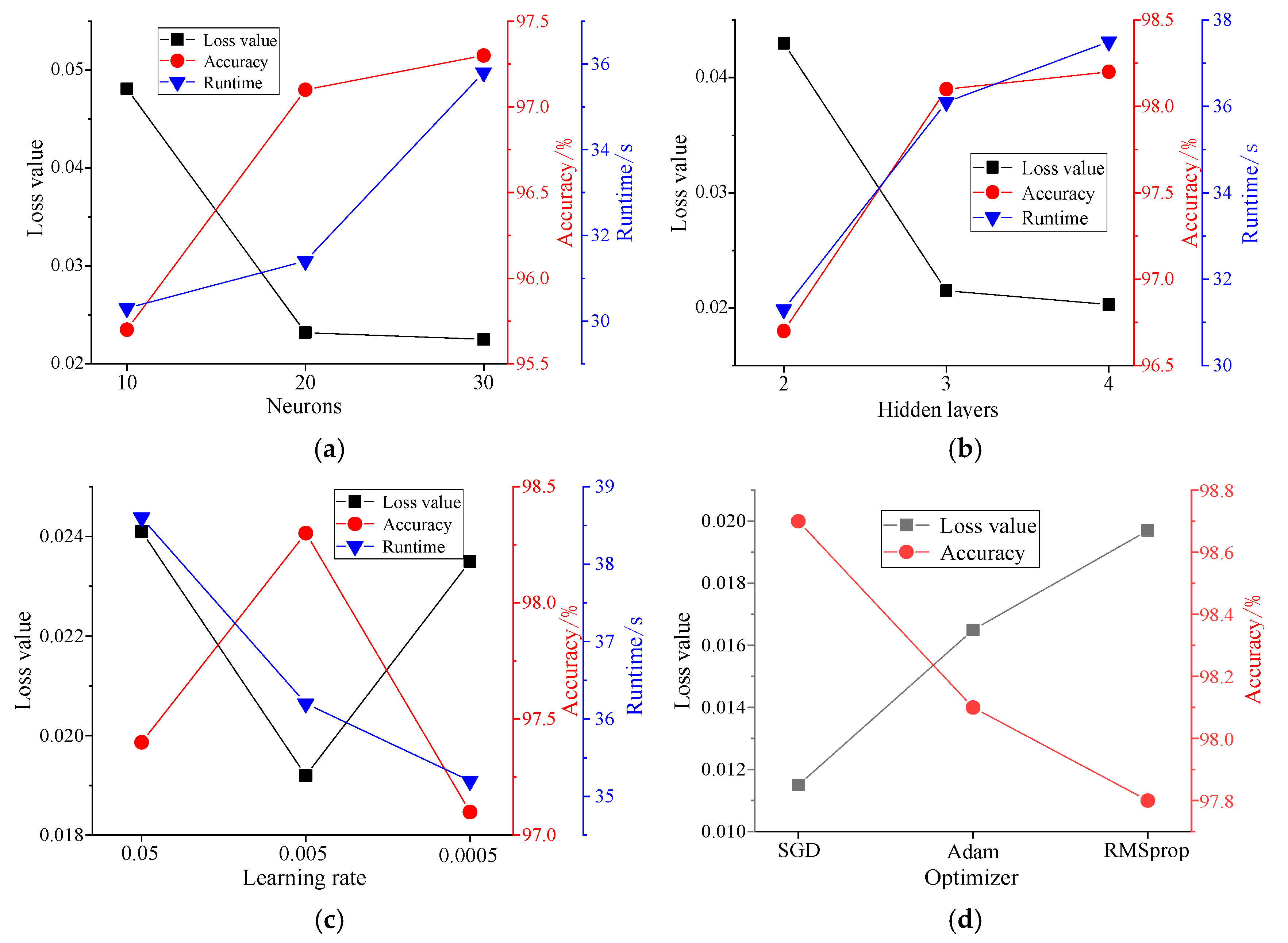
Training results for 10, 20, and 40 neurons, shown in Figure 13a, reveal that increasing neuron count enhances accuracy. A loss value of 0.0232 is achieved with 20 neurons, and further increasing the neuron count improves accuracy by only 2% when reaching 30 neurons. Thus, 20 neurons provide better training outcomes while optimising computational efficiency.

A comparison using 20 neurons with varying numbers of hidden layers is conducted, as shown in Figure 13b. The results indicate that increasing network depth reduces the loss value to 0.0207 with four hidden layers. However, the improvement in accuracy compared to the three-layer model is minimal, and it also introduces an increased risk of overfitting. Thus, three hidden layers are selected.

In addition, the comparison results for different learning rates and optimisers are presented in Figure 13c and Figure 13d, respectively. The optimisers compared include Stochastic Gradient Descent (SGD), Adaptive Moment Estimation (Adam), and Root Mean Square Propagation (RMSprop), which are widely used in deep learning for parameter optimisation with different convergence characteristics. The results indicate that model training is most effective with a learning rate of 0.005, while the validation accuracy is highest when the SGD optimiser is employed, reaching 98.7%.

Following the pre-training and validation of the network, appropriate hyperparameters can be selected for the subsequent training, validation, and testing of the models.

4.3. Training and Validation of Models

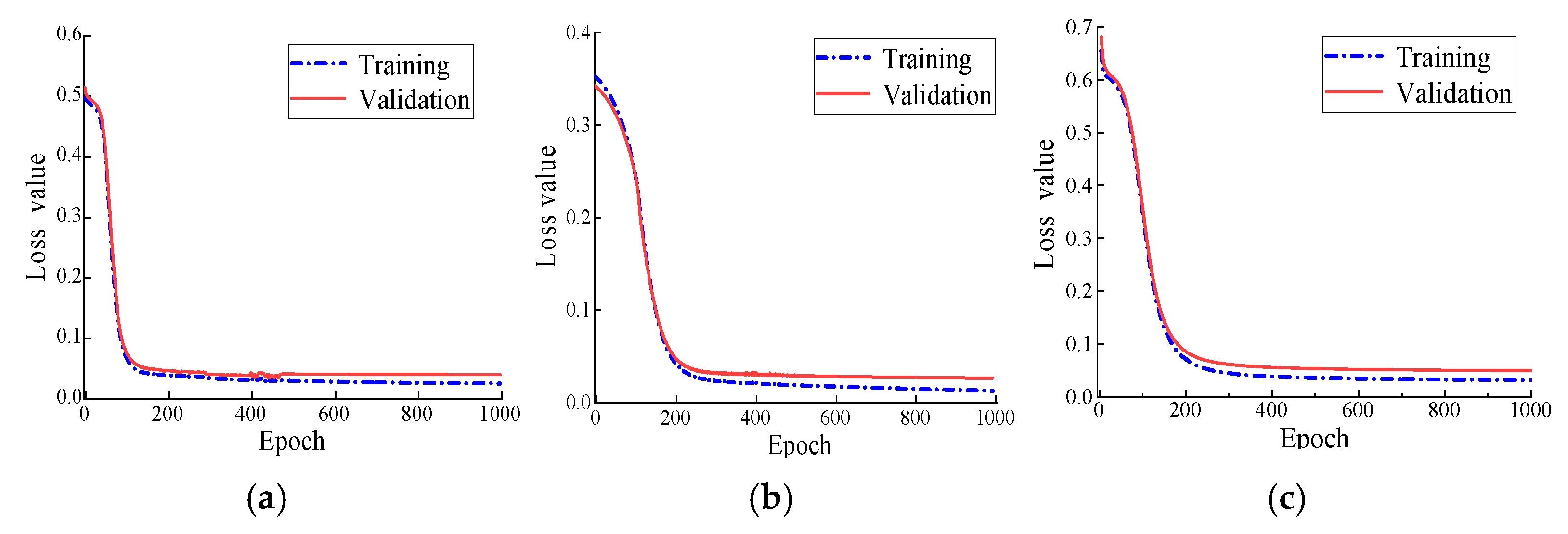
After completing one cycle of training for each model, the loss function values for the training set and validation set are obtained using Equation (5). The total number of training epochs is set to 1000, and the loss values for the training and validation phases across different epochs are illustrated in Figure 14 and summarised in

Table 4. Loss values for different training cycles.

Epoch	Model I		Model II		Model III
	Training Set	Validation Set	Training Set	Validation Set	Training Set	Validation Set
600	0.0061	0.0123	0.0071	0.0186	0.0064	0.0133
800	0.0055	0.0118	0.0065	0.0181	0.0059	0.0127
1000	0.0051	0.0115	0.0062	0.0176	0.0056	0.0122

. The validation set accuracy is presented in

Table 5. Results after 1000 epochs of model training.

Type	Accuracy of Training Set/%	Accuracy of Validation Set/%
Model I	99.3	98.7
Model II	98.6	97.8
Model III	99.1	98.3

.

The results indicate that after 1000 training cycles, the loss values of the validation set for the three models are 0.0115, 0.0176, and 0.0122, respectively. The corresponding accuracies of the validation set are 98.7%, 97.8%, and 98.3%. This indicates that the models achieve high accuracy following neural network training and exhibit strong robustness, faster convergence rates, and effective classification performance.

4.4. Testing and Evaluation of Models

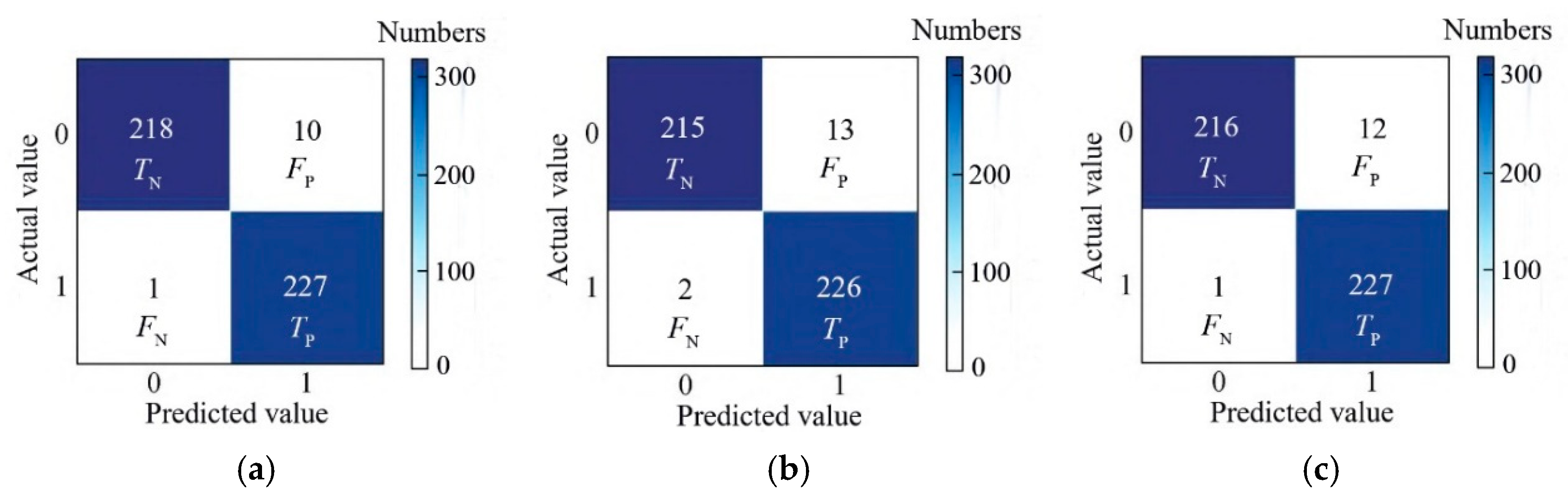
A separate test set, entirely distinct from the training and validation sets, is selected to evaluate their generalisation performance. For comparative analysis, the recognition results of the models are presented in the confusion matrix shown in Figure 15. Out of 456 test samples, the models correctly identified 445, 441, and 443 samples, respectively.

The results for the three models using the test set are compared in

Table 6. Evaluation metrics for models in the confusion matrix.

Deep Learning Model	Accuracy (Acc/%)	Precision (Pr/%)	Recall (Re/%)	F1 Score
Model I	97.6	95.8	99.6	0.975
Model II	96.8	94.6	99.1	0.968
Model III	97.3	95.0	99.6	0.972

. The results show that all three models achieve high test accuracy. Model I creates an accuracy of 97.6%, a recall rate of 99.6%, and an F₁ score of 0.975, reflecting optimal accuracy and robustness. As a result, it is preferred as the best recognition model in this paper. However, its accuracy is only 0.8% and 0.3% higher compared to Model II and Model III, respectively, suggesting that all three identification models show commendable generalisation performance. The identification model using AE features as inputs provides good recognition of seismic events. The trained model is well-suited for the real-time monitoring of rock AE signals, enabling the automatic warning of seismic events.

4.5. Identification Results of Seismic Events

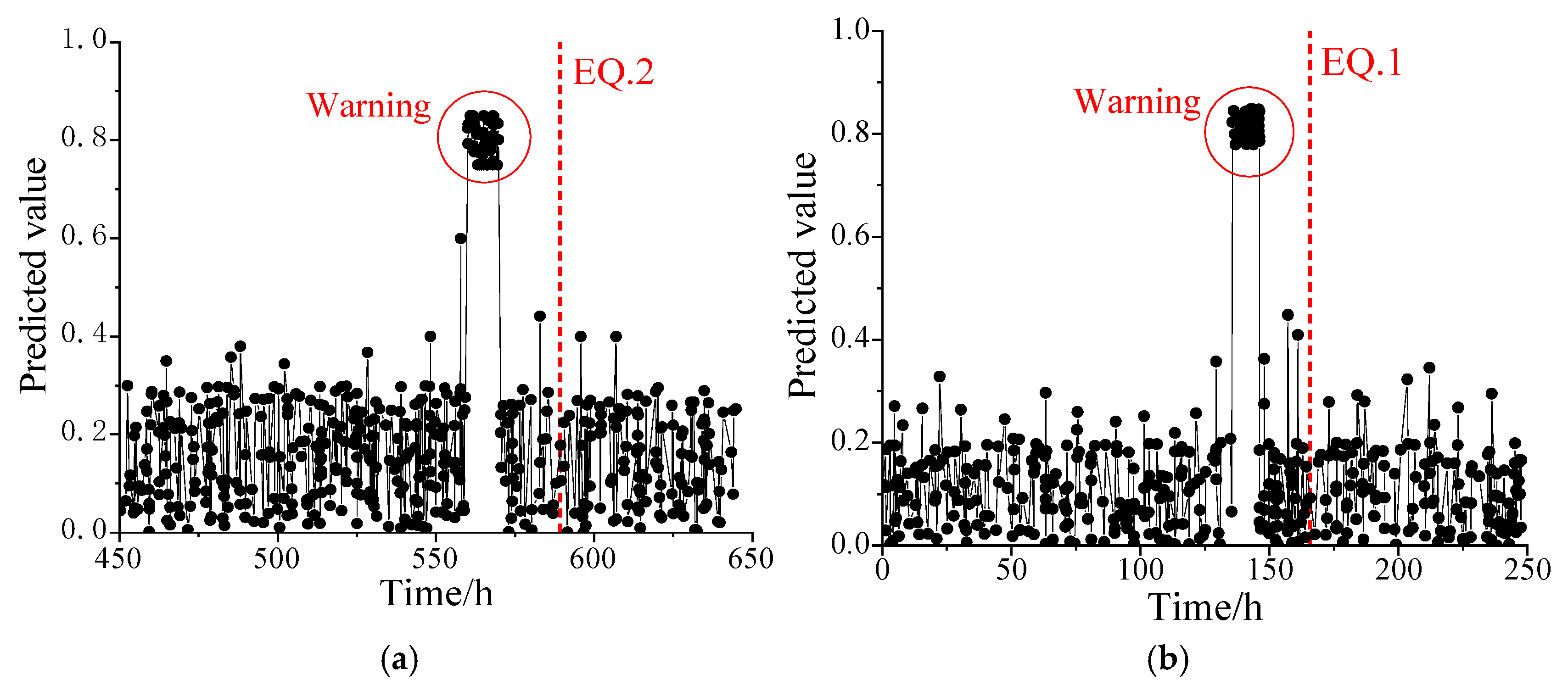
To evaluate the effectiveness of the models in identifying seismic events, we cross-test them with real-time data. Model II is evaluated with data from the EQ.2 earthquake, while Model III is tested with data from the EQ.1 earthquake. The cross-testing strategy (Model II on EQ.2 and Model III on EQ.1) is employed to verify that the models’ performance is robust across different earthquake events, not just the ones they are trained on.

The identification results of the models are presented in Figure 16. During the selected period, two warnings are issued, accurately corresponding to the two biggest seismic events that occur within that timeframe. This demonstrates the model’s high identification accuracy for significant seismic events.

4.6. Comparison with Various Machine Learning Models

As a comparative study, the proposed deep learning model is experimentally evaluated against traditional machine learning models, including Support Vector Machine (SVM), Light GBM (LGB), and Random Forest (RF). SVM is a supervised learning method that classifies data into two classes by finding an optimal hyperplane that maximises the margin between them; the LGB model, an enhanced gradient boosting decision tree algorithm, combines unilateral gradient sampling and mutually exclusive feature bundling; and the RF model is a bagging ensemble algorithm that builds training subsets through random sampling, trains individual decision trees, and derives final predictions through majority voting.

Table 7. Testing results of various machine learning models.

Identification Model	Accuracy (Acc/%)	Precision (Pr/%)	Recall (Re/%)	F1 Score
Deep learning	97.6	95.8	99.6	0.975
SVM	95.3	94.3	96.2	0.952
LGB	94.6	95.2	94.5	0.948
RF	93.2	93.4	92.7	0.930

presents the test results for the SVM, LGB, and RF models. The RF model shows the lowest accuracy at 93.2%, followed by the LGB model at 94.6% and the SVM model at 95.3%. In contrast, the deep learning model achieves higher accuracy, with F₁ scores surpassing the SVM, LGB, and RF models by 2.6%, 3.1%, and 5.1%, respectively. These results emphasise the deep learning model’s capability to extract hidden features from complex data and enhance generalisation through the backpropagation algorithm. For earthquake early warning, the model using AE features as inputs achieves remarkable accuracy and robustness in identifying seismic events compared to traditional machine learning algorithms. Hence, the trained model is well-suited for online monitoring and early warning of rock AE signals.

5. Discussion

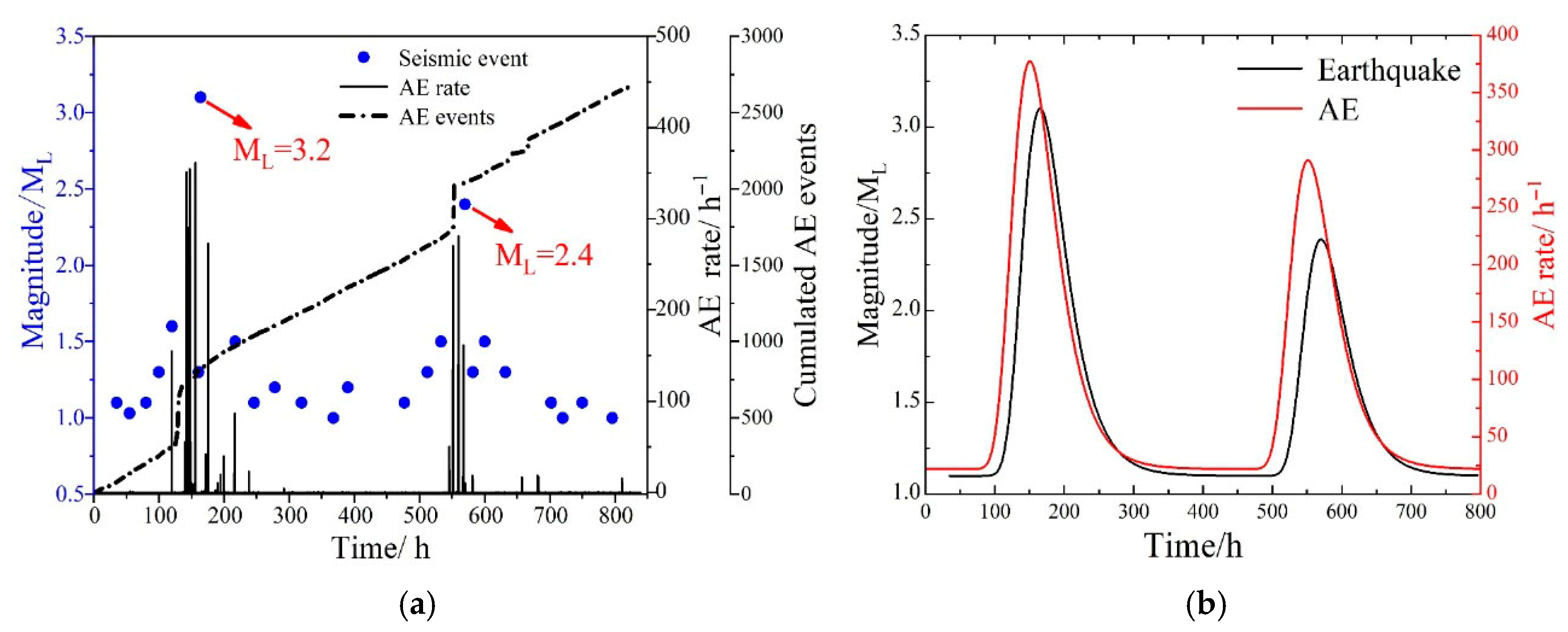
While this study presents a novel approach to earthquake precursor detection using AE signals and deep learning, we acknowledge several limitations that warrant discussion. First, the 35-day monitoring period, though sufficient for demonstrating proof-of-concept, represents only a snapshot of seismic activity in the region. The two target events (M_L = 3.2 and M_L = 2.4) provided clear AE precursor patterns, but longer-term monitoring is essential to establish statistical robustness and account for potential variability in precursor signals across different seismic cycles. For instance, seasonal changes in groundwater levels or tectonic stress accumulation rates could influence AE characteristics, and these factors cannot be assessed within our short observation window.

Second, the limited number of seismic events in our dataset restricts the model’s ability to generalise across a broader magnitude range. While the deep learning algorithm achieved high accuracy (97.6%) for the recorded events, its performance for less frequent but potentially more destructive earthquakes (e.g., M_L > 5.0) remains untested. Additionally, the absence of weaker events (0 < M_L < 1.0) in our analysis leaves open questions about whether micro-seismic activity shares precursor features with larger earthquakes or represents a distinct phenomenon. Future studies should prioritise extended monitoring to capture these less frequent but critical scenarios.

The observed AE precursors correlated with seismic events within a 100~200 km radius; however, the spatial effectiveness of precursors may scale with earthquake magnitude and crustal stress distribution, necessitating long-term multi-site monitoring.

To address these limitations, the research will adopt a phased implementation approach. In the short term, an expanded network of AE sensors will be strategically deployed across geologically diverse sites in eastern Guangdong to acquire comprehensive datasets under varying subsurface conditions. Subsequent long-term monitoring (3–5 years) will systematically examine the correlation between AE patterns and seismic events across the full magnitude spectrum, with particular attention to potential environmental confounders. The methodology’s application in other seismically active regions could further elucidate the differentiation between universal precursor characteristics and region-specific signatures. While the present findings represent an initial proof-of-concept, they provide a substantive framework for advancing the development of next-generation earthquake early-warning systems.

6. Conclusions

This paper focuses on the real-time monitoring and precursor identification of seismic events in high-intensity areas. Field tests in mountain tunnels are conducted to study the AE features of earthquake precursors. A rapid earthquake warning method based on rock AE detection and deep learning is proposed, providing a reference for seismic early warning and mitigation. The main conclusions are as follows:

(1)

The time-series features captured by the AE equipment in real time, including AE event, rate, frequency, and amplitude, provide a basis for the rapid identification of seismic events. The multi-peak statistical analysis reveals a strong correlation between AE and nearby seismic activity. The trend in AE temporal distribution precedes that of earthquakes, serving as precursors that can identify main earthquakes 17 h in advance.

(2)

The extracted AE features serve as samples, while the acquired seismic data act as labels for constructing the deep learning model. The high validation accuracy and recognition accuracy indicate that the deep learning model is not only more accurate but also exhibits better generalisation and robustness compared to traditional machine learning algorithms.

(3)

Deep learning has advanced the ability to identify earthquakes rapidly. The earthquake precursor identification model, which uses AE features as inputs, effectively recognises seismic events and successfully identified the two biggest seismic events during the monitoring period. This model has practical value in the field, allowing for real-time monitoring and automated warning of seismic events.

To strengthen the identification reliability, future studies will prioritise long-term monitoring and incorporate data from larger-magnitude earthquakes. This will help refine precursor signatures, reduce false alarms, and enhance the model’s robustness for real-world early-warning systems.

References

1. Chien, S.; Chi, W.; Ke, C. Precursory and coseismal groundwater temperature perturbation: An example from Taiwan. J. Hydrol. 2020, 582, 124457. [Google Scholar] [CrossRef]
2. Singh, P.; Mukherjee, S. Chemical signature detection of groundwater and geothermal waters for evidence of crustal deformation along fault zones. J. Hydrol. 2020, 582, 124459. [Google Scholar] [CrossRef]
3. Li, N.; Kong, X.; Lin, L. Anomalies in continuous GPS data as precursors of 15 large earthquakes in western north america during 2007–2016. Earth Sci. Inform. 2020, 13, 163–174. [Google Scholar] [CrossRef]
4. Yusof, K.A.; Abdullah, M.; Hamid, N.S.A.; Ahadi, S.; Yoshikawa, A. Correlations between earthquake properties and features of possible ulf geomagnetic precursor over multiple earthquakes. Universe 2021, 7, 20. [Google Scholar] [CrossRef]
5. Jiang, Z.; Zhu, Z.; Lacidogna, G. AE monitoring of crack evolution on UHPC deck layer of a long-span cable-stayed bridge. Dev. Built Environ. 2025, 23, 100697. [Google Scholar] [CrossRef]
6. Zhu, Z.; Jiang, Z.; Accornero, F. Size-scale and time-scale effects on the failure of UHPC-strengthened reinforced concrete beams. Structures 2025, 78, 109248. [Google Scholar] [CrossRef]
7. Jiang, Z.; Zhu, Z.; Accornero, F. Tensile-to-shear crack transition in the compression failure of steel-fibre-reinforced concrete: Insights from acoustic emission monitoring. Buildings 2024, 14, 2039. [Google Scholar] [CrossRef]
8. Carpinteri, A.; Borla, O. Fracto-emissions as seismic precursors. Eng. Fract. Mech. 2017, 177, 239–250. [Google Scholar] [CrossRef]
9. Lei, X.L.; Ma, S. Laboratory acoustic emission study for earthquake generation process. Earthq. Sci. 2014, 27, 627–646. [Google Scholar] [CrossRef]
10. Gregori, G.P.; Poscolieri, M.; Paparo, G.; De Simone, S.; Rafanelli, C.; Ventrice, G. “Storms of crustal stress” and AE earthquake precursors. Nat. Hazards Earth Syst. Sci. 2010, 10, 319–337. [Google Scholar] [CrossRef]
11. Lacidogna, G.; Carpinteri, A.; Manuello, A.; Durin, G.; Schiavi, A.; Niccolini, G.; Agosto, A. Acoustic and electromagnetic emissions as precursor phenomena in failure processes. Strain 2011, 47, 144–152. [Google Scholar] [CrossRef]
12. Carpinteri, A.; Lacidogna, G.; Manuello, A.; Niccolini, G. A study on the structural stability of the Asinelli Tower in Bologna. Struct. Control Health Monit. 2016, 23, 659–667. [Google Scholar] [CrossRef]
13. Zimatore, G.; Garilli, G.; Poscolieri, M.; Rafanelli, C.; Gizzi, F.T.; Lazzari, M. The remarkable coherence between two Italian far away recording stations points to a role of acoustic emissions from crustal rocks for earthquake analysis. Chaos 2017, 27, 043101. [Google Scholar] [CrossRef]
14. Carpinteri, A.; Lacidogna, G.; Niccolini, G. Acoustic emission monitoring of medieval towers considered as sensitive earthquake receptors. Nat. Hazards Earth Syst. Sci. 2007, 7, 251–261. [Google Scholar] [CrossRef]
15. Lacidogna, G.; Cutugno, P.; Niccolini, G.; Invernizzi, S.; Carpinteri, A. Correlation between earthquakes and AE monitoring of historical buildings in seismic areas. Appl. Sci. 2015, 5, 1683–1698. [Google Scholar] [CrossRef]
16. Gregori, G.P.; Paparo, G.; Poscolieri, M.; Zanini, A. Acoustic emission and released seismic energy. Nat. Hazards Earth Syst. Sci. 2005, 5, 777–782. [Google Scholar] [CrossRef]
17. Carpinteri, A.; Borla, O. Acoustic, electromagnetic, and neutron emissions as seismic precursors: The lunar periodicity of low-magnitude seismic swarms. Eng. Fract. Mech. 2019, 210, 29–41. [Google Scholar] [CrossRef]
18. Lukovenkova, O.; Solodchuk, A.; Tristanov, A.; Malkin, E.; Salikhov, N.; Shevtsov, B.; Vilayev, A. Complex analysis of pre-seismic geoacoustic and electromagnetic emission signals. In Proceedings of the E3S Web of Conferences, Milan, Italy, 13–15 February 2019; p. 03001. [Google Scholar]
19. Spivak, A.; Rybnov, Y. Acoustic effects of strong earthquakes. Izv. Phys. Solid Earth 2021, 57, 37–45. [Google Scholar] [CrossRef]
20. Wang, X.; Wang, Z.; Wang, B.; Zhang, H.; Wu, Y.; Li, S.; Xia, Q.; Zhang, Y.; Feng, F.; Wu, X. Deep-learning image processing of interferometric particle imaging in icing wind tunnel. Measurement 2025, 245, 116324. [Google Scholar] [CrossRef]
21. Yin, X.; Liu, Q.; Lei, J.; Pan, Y.; Huang, X.; Lei, Y. Hybrid deep learning-based identification of microseismic events in TBM tunnelling. Measurement 2024, 238, 115381. [Google Scholar] [CrossRef]
22. Mignan, A.; Broccardo, M. Neural network applications in earthquake prediction (1994–2019): Meta-analytic and statistical insights on their limitations. Seismol. Res. Lett. 2020, 91, 2330–2342. [Google Scholar] [CrossRef]
23. Ida, Y.; Ishida, M. Analysis of seismic activity using self-organizing map: Implications for earthquake prediction. Pure Appl. Geophys. 2022, 179, 1–9. [Google Scholar] [CrossRef]
24. Seydoux, L.; Balestriero, R.; Poli, P.; de Hoop, M.; Campillo, M.; Baraniuk, R. Clustering earthquake signals and background noises in continuous seismic data with unsupervised deep learning. Nat. Commun. 2020, 11, 3972. [Google Scholar] [CrossRef] [PubMed]
25. Ma, S.; Li, Z.; Wang, W. Machine learning of source spectra for large earthquakes. Geophys. J. Int. 2022, 231, 692–702. [Google Scholar] [CrossRef]
26. Al Banna, M.H.; Ghosh, T.; Al Nahian, M.J.; Taher, K.A.; Kaiser, M.S.; Mahmud, M.; Hossain, M.S.; Andersson, K. Attention-based bi-directional long-short term memory network for earthquake prediction. IEEE Access 2021, 9, 56589–56603. [Google Scholar] [CrossRef]
27. Jozinović, D.; Lomax, A.; Štajduhar, I.; Michelini, A. Transfer learning: Improving neural network-based prediction of earthquake ground shaking for an area with insufficient training data. Geophys. J. Int. 2022, 229, 704–718. [Google Scholar] [CrossRef]
28. Kail, R.; Burnaev, E.; Zaytsev, A. Recurrent convolutional neural networks help to predict the location of earthquakes. IEEE Geosci. Remote Sens. Lett. 2021, 19, 1–5. [Google Scholar] [CrossRef]
29. Fuentes, A.G.; Nicolis, O.; Peralta, B.; Chiodi, M. Spatio-temporal seismicity prediction in Chile using a multi-column convlstm. IEEE Access 2022, 10, 107402–107415. [Google Scholar] [CrossRef]
30. Pu, Y.; Chen, J.; Apel, D. Deep and confident prediction for a laboratory earthquake. Neural Comput. Appl. 2021, 33, 11691–11701. [Google Scholar] [CrossRef]
31. Geng, Y.; Su, L.; Jia, Y.; Han, C. Seismic events prediction using deep temporal convolution networks. J. Electr. Comput. Eng. 2019, 2019, 7343784. [Google Scholar] [CrossRef]
32. Wang, Q.; Guo, Y.; Yu, L.; Li, P. Earthquake prediction based on spatio-temporal data mining: An lstm network approach. IEEE Trans. Emerg. Top. Comput. 2017, 8, 148–158. [Google Scholar] [CrossRef]
33. Shcherbakov, R.; Zhuang, J.; Zöller, G.; Ogata, Y. Forecasting the magnitude of the largest expected earthquake. Nat. Commun. 2019, 10, 4051. [Google Scholar] [CrossRef]
34. Devries, P.M.R.; Viégas, F.; Wattenberg, M.; Meade, B.J. Deep learning of aftershock patterns following large earthquakes. Nature 2018, 560, 632–634. [Google Scholar] [CrossRef] [PubMed]
35. Ahmadzadeh, M.; Zahrai, S.M.; Bitaraf, M. An integrated deep neural network model combining 1D CNN and LSTM for structural health monitoring utilizing multisensory time-series data. Struct. Health Monit. 2025, 24, 447–465. [Google Scholar] [CrossRef]
36. Dalhat, M. Deep Neural Network modeling and analysis of the laboratory compaction parameter of unbound granular materials. Measurement 2025, 244, 116488. [Google Scholar] [CrossRef]
37. Luque, A.; Carrasco, A.; Martín, A.; de las Heras, A. The impact of class imbalance in classification performance metrics based on the binary confusion matrix. Pattern Recognit. 2019, 91, 216–231. [Google Scholar] [CrossRef]
38. Zhu, Z.; Jiang, Z.; Accornero, F.; Carpinteri, A. Correlation between seismic activity and acoustic emission on the basis of in situ monitoring. Nat. Hazards Earth Syst. Sci. 2024, 24, 4133–4143. [Google Scholar] [CrossRef]
Figure 1. Method for identifying earthquake precursors.
Sci 07 00103 g001
Figure 2. Deep neural network based on Pytorch framework.
Sci 07 00103 g002
Figure 3. Training process of deep learning model.
Sci 07 00103 g003
Figure 4. Location of test tunnel: (a) satellite map; (b) mountain tunnel location; (c) tunnel entrance.
Sci 07 00103 g004
Figure 5. Monitoring system layout: (a) tunnel interior; (b) AE acquisition system; (c) seismometer.
Sci 07 00103 g005
Figure 6. Seismicity in the area around Shantou City: (a) historical seismic activity; (b) main seismic events during monitoring [38].
Sci 07 00103 g006
Figure 7. Gaussian distribution of seismic events: (a) Gaussian parameters; (b) seismic distribution.
Sci 07 00103 g007
Figure 8. Rock AE detection technology: (a) Schematic diagram; (b) acoustic wave features.
Sci 07 00103 g008
Figure 9. Temporal correlation between AE and seismic events: (a) AE and seismic event time series; (b) Gaussian distribution.
Sci 07 00103 g009
Figure 10. AE features before the earthquake: (a) AE event (feature x1); (b) AE rate (feature x2); (c) frequency (feature x3); (d) amplitude (feature x4).
Sci 07 00103 g010
Figure 11. Construction process of the dataset.
Sci 07 00103 g011
Figure 12. Schematic diagram of deep learning models.
Sci 07 00103 g012
Figure 13. Validation results for different network parameters: (a) number of neurons; (b) number of hidden layers; (c) learning rate; (d) optimiser type.
Sci 07 00103 g013
Figure 14. Loss values during training and validation phases: (a) Model I; (b) Model II; (c) Model III.
Sci 07 00103 g014
Figure 15. Calculation of confusion matrix for test sets: (a) Model I; (b) Model II; (c) Model III.
Sci 07 00103 g015
Figure 16. Identification performance of deep learning model: (a) warning results of EQ.2; (b) warning results of EQ.1.
Sci 07 00103 g016