Monitoring the Distance and Velocity of Protons in a Medium for Biomedical Applications Using a Straightforward Mathematical Approach

Abstract

Radiotherapy is one of the major cancer treatments that uses controlled doses of ionizing radiation to damage tumor cells. The monitoring of charged particles within a medium is of tremendous importance in radiotherapy. Monte Carlo methods can be used to estimate radiation profiles; however, despite their effectiveness, they are computationally expensive, which limits their practicality. To simplify the analysis, approximate analytical methods focused on estimating the range of charged particles and their velocity function within a medium have been previously derived. Previous solutions include non-elementary functions, such as the exponential integral function with relativistic coordinate transformations, or the use of regular perturbation methods accounting for small relativistic effects. In this paper, a much simpler approach is presented to assist practitioners in the field of radiotherapy. Using the proposed method, the particles’ range and velocities are calculated exclusively with elementary functions. The main advantage of the proposed approach, aside from its straightforward application, is its suitability for relativistic velocities. The equations derived in this paper were successfully tested at the radiotherapy level, accommodating protons with energies of up to 350 MeV.

1. Introduction

According to statistics from the World Health Organization (WHO), cancer ranks as the second leading cause of death worldwide [1]. It is estimated that approximately 10 million deaths from cancer occur each year [1,2]. Over the past century, external beam energy for cancer treatment has steadily advanced, resulting in the development of two primary approaches. The first, radiotherapy, uses X-ray, gamma, and proton beams to induce ionizing damage [1,2,3,4,5,6,7,8,9]. The second, photodynamic therapy, relies on photons to activate photosensitizers, producing reactive oxygen species that cause cytotoxic effects [10,11,12,13]. For decades, these two therapies evolved separately: photodynamic therapy has been applied to treat surface tumors, while radiotherapy has been directed toward deeper tumors [1]. In recent years, efforts to combine radiotherapy and photodynamic therapy have intensified, resulting in the development of innovative techniques such as X-ray photodynamic therapy [14] and proton-induced photodynamic therapy [15]. For example, Grigalavicius et al. [15] demonstrated that proton beams can activate fluorescence and singlet oxygen ¹O₂ in photosensitizers for proton-induced photodynamic therapy (PrDT). It has been suggested that the photosensitizers increased the interaction cross-section, leading to accelerated high-energy deposition [15]. Therefore, monitoring the charged particles traveling within the tissue is crucial for classic radiotherapy approaches and new cutting-edge therapeutic procedures.

It is important to note that one of the key challenges associated with the medical procedures mentioned above is effectively modeling tissue-particle interactions and the computational resources required for this task. Accurate modeling of radiation interactions is essential for various applications. To fully harness the potential of charged particles, a thorough understanding of energy deposition across different media is critical. Monte Carlo techniques are commonly used to achieve this [16]. Monte Carlo particle transport packages are highly advanced tools capable of simulating the interaction of particle radiation with matter as it passes through a medium [17,18,19,20]. These approaches can capture system behavior across all scales, including secondary and higher-order interactions, but they are computationally expensive with significant evaluation times [20]. In other words, although Monte Carlo methods have been highly successful in modeling these more complex target materials, they come with a significant computational cost, particularly when the problem is time-dependent [20]. The goal of this work is to develop a new simple model that accurately captures the general behavior of charged particles within the energy ranges relevant to therapy (up to 350 MeV). It is important to note that approximate analytical solutions to this problem have been proposed previously [20,21]. Grimes et al. [20] provided an analytical solution for the velocities of charged particles with respect to the distance traveled in a medium, expressed in terms of the inverse exponential function with relativistic coordinate transformations. This is not a standard function, and no closed-form expression exists for it [20]. The solution is perfectly executed and accurate, as it is valid for relativistic velocities; however, its use requires a strong mathematical and physical background.

An alternative solution has also been presented by Martinez et al., who provided a series solution (based on regular perturbation methods) for the range and dose distribution that does not include the inverse exponential function [21]. This solution is accurate when considering small relativistic effects. By including a large number of terms in the series solution, the application of the results can be extended to protons with energies up to 200 MeV.

Both the results of Grimes et al. and Martinez et al. are based on solving the Bethe equation below:

$$-{\displaystyle \frac{dE}{dx}}={\displaystyle \frac{4\pi n{z}^2}{m_e}}{\left({\displaystyle \frac{e^2}{4\pi {\epsilon }_0}}\right)}^2\left[{\displaystyle \frac{1}{v^2\left(x\right)}}\right]\left\{\left.\mathrm{l}\mathrm{n}\left[{\displaystyle \frac{2m_e{v}^2\left(x\right)}{I\left(1-{\beta }^2\right)}}\right]-{\beta }^2\right\}\right.$$

(1)

where n is the electron density of the material, e is the electron charge, m_e is the electron mass, I is the mean excitation potential, z is the multiple of the electron charge, and $\beta =v\left(x\right)/c$, where $v$ is the speed of the particle and $c$ is the speed of light in a vacuum. It is important to highlight that a particle’s energy depends on its speed, which, in turn, is a function of distance $x$. Since the energy levels relevant to radiotherapy are considered, the relativistic definition of particle kinetic energy should be used. This definition is expressed in terms of the Lorentz factor [20]:

$$E={(\gamma -1)m}_p{c}^2 , \gamma ={\left(1-{\beta }^2\right)}^{-{\displaystyle \frac{1}{2}}} , \beta ={\displaystyle \frac{v}{c}}$$

(2)

According to Grimes et al. [20], Equation (1) can be simplified as follows:

$$-{\displaystyle \frac{dE}{dx}}={\displaystyle \frac{4\pi n{z}^2}{m_e}}{\left({\displaystyle \frac{e^2}{4\pi {\epsilon }_0}}\right)}^2\left[{\displaystyle \frac{1}{v^2\left(x\right)}}\right]\ln \left[{\displaystyle \frac{2m_e{v}^2\left(x\right)}{I}}\right]=A{m}_p{\displaystyle \frac{\ln \left[B{v}^2\left(x\right)\right]}{v^2\left(x\right)}}$$

(3)

where $A={\displaystyle \frac{4\pi n{z}^2}{m_e{m}_p}}{\left({\displaystyle \frac{e^2}{4\pi {\epsilon }_0}}\right)}^2$ and $B={\displaystyle \frac{2m_e}{I}}$. The approximate Equation (3) results in negligible error when applied to energies relevant to radiotherapy. In particular, when using Equation (3) instead of (1), there is an error of approximately 1% for high-energy protons (250 MeV) [1]. The procedure employed by Grimes et al. [20] to derive the function $v\left(x\right)$ is described as follows: using the chain rule, they resulted in

$${\displaystyle \frac{dE}{dx}}={\displaystyle \frac{dE}{dv}}{\displaystyle \frac{dv}{dx}}=m_{p}v\left(x\right){\gamma }^3\left(v\right){\displaystyle \frac{dv}{dx}}$$

(4)

Subsequently, by substituting Equation (4) into Equation (3), it is easily concluded that

$$A{\displaystyle \frac{\ln \left[B{v}^2\left(x\right)\right]}{v^3\left(x\right)}}=-{\gamma }^3\left(v\right){\displaystyle \frac{dv}{dx}}$$

(5)

By solving the above differential equation, the range of the charged particles can be determined [20]. However, the strategies employed in previous publications [20,21] require advanced mathematical tools, special functions [20], or include series solutions, with results limited to protons with energies up to 200 MeV [21]. While these approaches are of significant mathematical interest from both theoretical and applied physics, as well as biomedical engineering perspectives, they may have limited practical applicability for radiotherapy professionals or young researchers in medicine and biomedical technology who lack experience with advanced mathematical procedures.

The goal of this paper is to simplify the procedure for approximately determining the function $v\left(x\right)$ while simultaneously deriving straightforward, easily adaptable solutions for the range of particles in a medium. We demonstrate that the range of charged particles within a medium and their velocity as a function of distance can be described by elementary functions, with appropriate coefficients depending on the particles’ initial energy. The analysis presented in this paper focuses on protons, as they are used in both radiotherapy and new combined therapeutic practices, as previously mentioned. However, these methods can equally be applied to any charged particle.

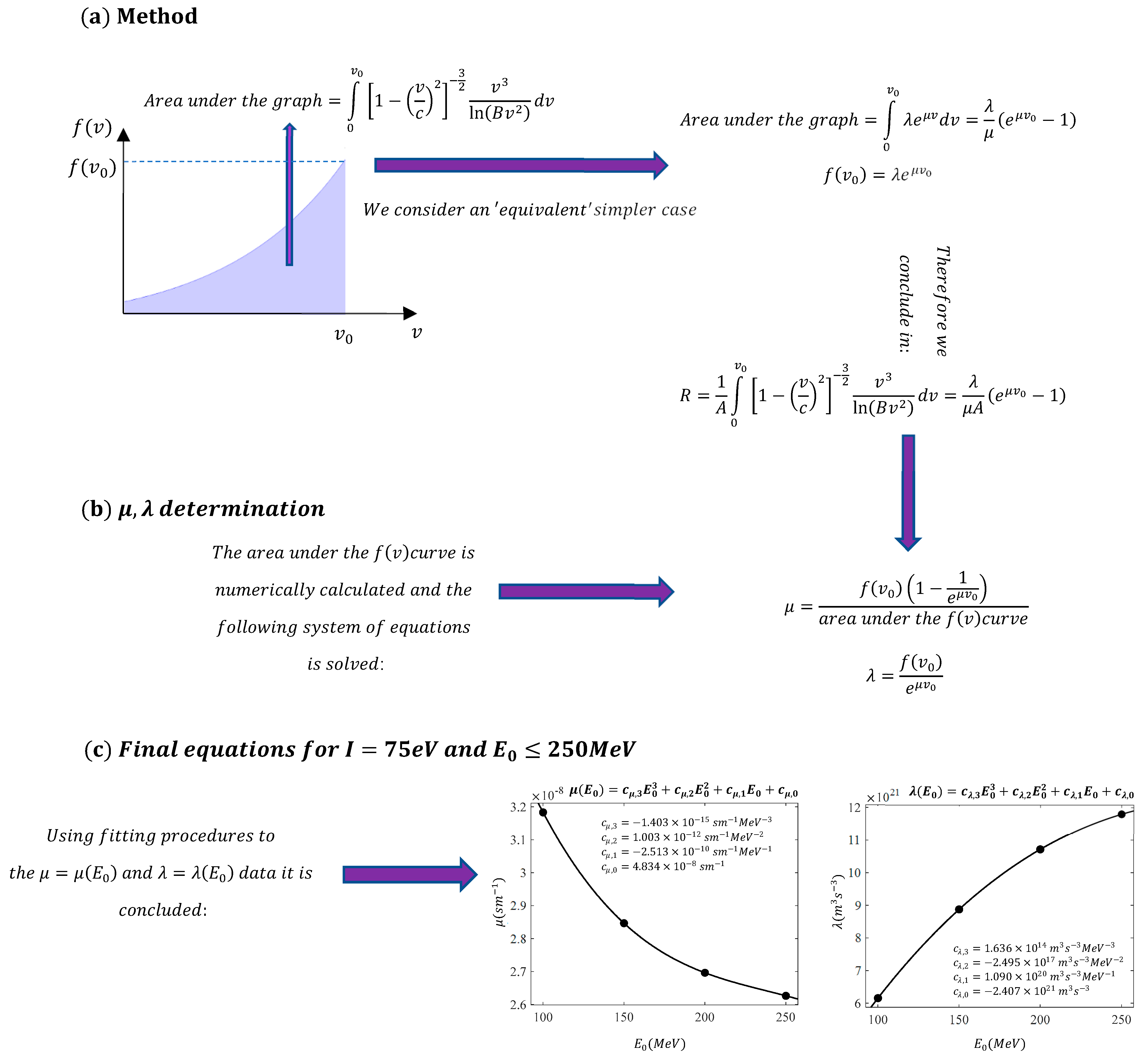
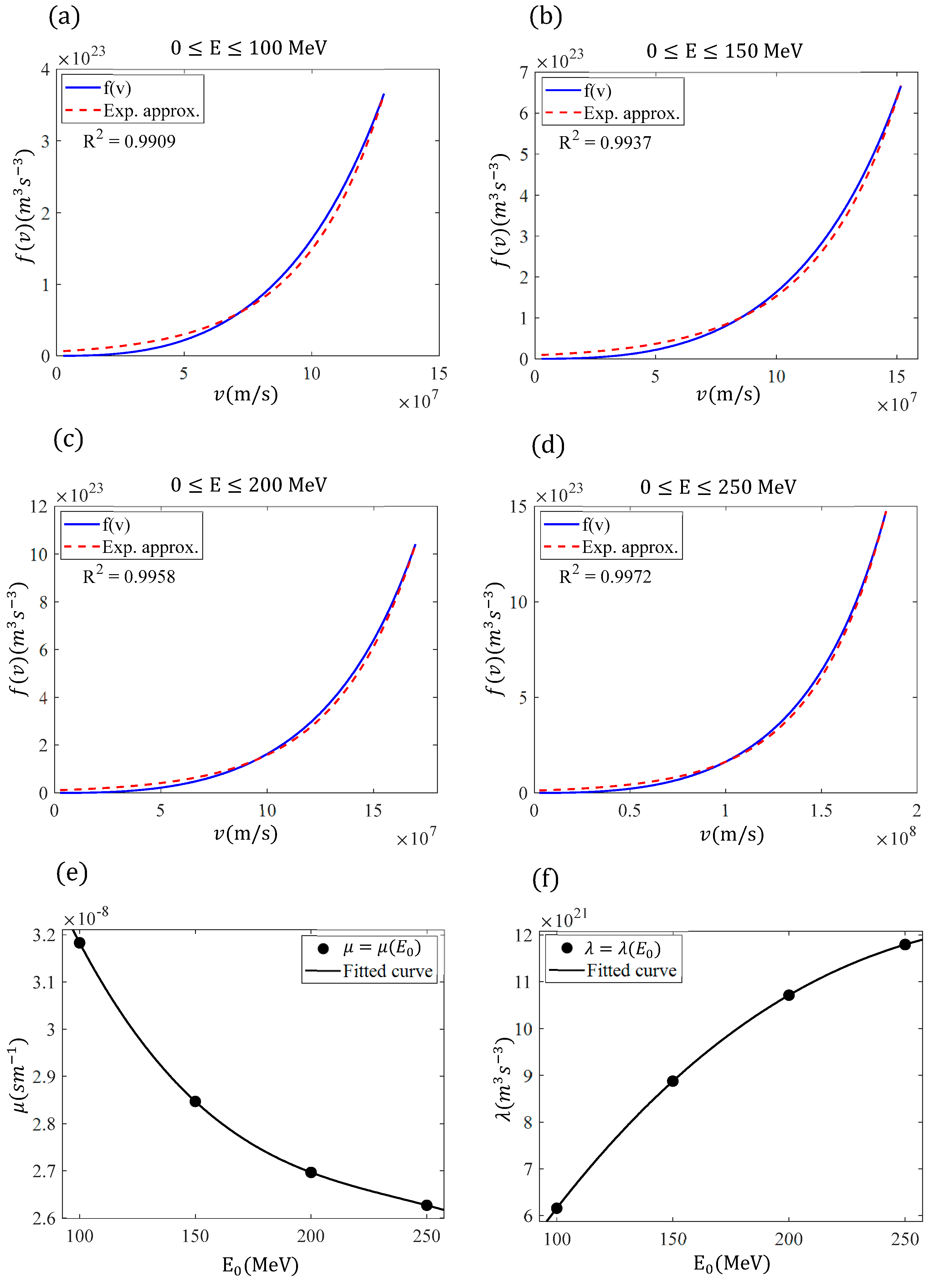
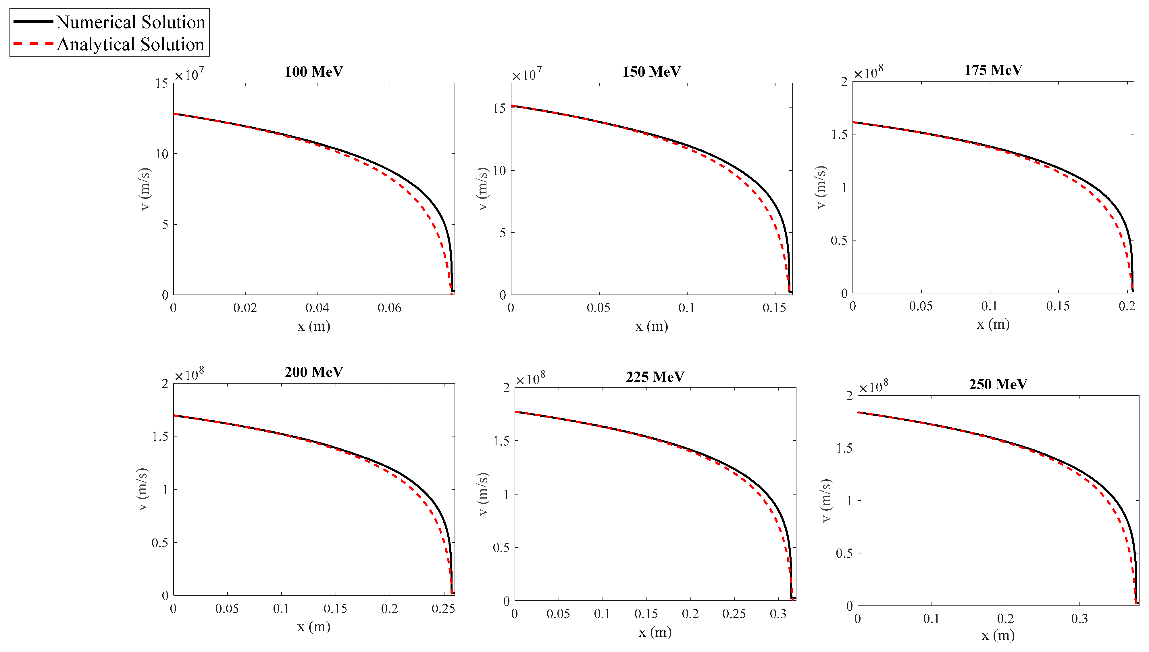
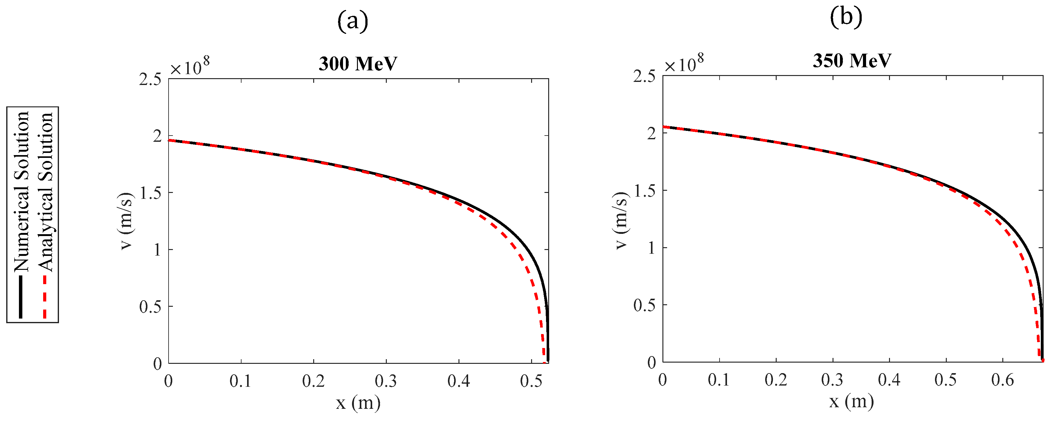
This paper is organized as follows: In Section 2 (Materials and Methods), we derive a simple equation for the range of the charged particles. The approach to avoiding the extreme mathematical complexity of this problem is to identify an ‘equivalent’ simpler problem using fitting methods that employ basic exponential functions. In Section 3 (Results), the newly derived equation is tested, and the results are compared with other analytical and experimental findings from the literature, as well as with exact numerical results. In addition, the function $v=f\left(x\right)$ is derived based on the simple exponential approximation introduced in Section 2, where $v$ is the velocity of the protons with respect to the distance traveled $x$. Furthermore, the case of protons with very large initial energies (>250 MeV) is considered. In Section 4 (the Discussion Section), further insights regarding small initial energies and the uncertainties in the associated variables are also presented, emphasizing their impact on the derived equations and the analytical results.

2. Materials and Methods

2.1. A Simple Exponential Approximation

Particle’s range is defined as below [20,22,23]:

$$R=\underset{v_0}{\overset{0}{\int }}{\displaystyle \frac{dx}{dv}}dv$$

(6)

Equation (6) simply provides the maximum distance traveled by the charged particles in a medium. By substituting Equation (5) into Equation (6), it is concluded that

$$R=-{\displaystyle \frac{1}{A}}\underset{v_0}{\overset{0}{\int }}{\left[1-{\left({\displaystyle \frac{v}{c}}\right)}^2\right]}^{-{\displaystyle \frac{3}{2}}}{\displaystyle \frac{v^3}{\ln \left(B{v}^2\right)}}dv={\displaystyle \frac{1}{A}}\underset{0}{\overset{v_0}{\int }}f\left(v\right)dv$$

(7)

where

$${f\left(v\right)=\left[1-{\left({\displaystyle \frac{v}{c}}\right)}^2\right]}^{-{\displaystyle \frac{3}{2}}}{\displaystyle \frac{v^3}{\ln \left(B{v}^2\right)}}$$

(8)

Integrating the function $f\left(v\right)$ as appears in Equation (7) is not trivial [20]. Additionally, the solution involves the inverse exponential function, as previously mentioned, which is not an elementary function. The idea behind simplifying the mathematical procedure and, most importantly, the final result regarding the particle’s range in a medium is to ‘fit’ a simpler, easily integrable function to the values of $f\left(v\right)$. Many elementary functions, such as exponentials, power law functions, and polynomial functions, were tested in the range $0\le v\le v_0$, where ${0.4281c\le v}_0\le 0.6847c$ and $c$ is the speed of light in vacuum. The values $0.4281c$ and $0.6847c$ are associated with protons having energies equal to 100 MeV and 350 MeV (i.e., within the energy range that is used in radiotherapy). The simplest function that best fit the data was found to be the function $\lambda e^{\mu v}$, i.e.,

$$f\left(v\right)={\left[1-{\left({\displaystyle \frac{v}{c}}\right)}^2\right]}^{-{\displaystyle \frac{3}{2}}}{\displaystyle \frac{v^3}{\ln \left(B{v}^2\right)}}\cong \lambda e^{\mu v}$$

(9)

In Equation (9), $\lambda$ and $\mu$ are parameters that depend only on the initial speed of the charged particles (or, alternatively, on their initial energy). However, for a given initial energy, they remain constant as the particle travels through a medium and its velocity decreases. The rationale behind the approximation presented in Equation (9) is that, since $f\left(v\right)$ is a monotonically increasing function, we searched for the simplest function that satisfies this criterion in order to make it easily integrable. With the appropriate parameters μ and λ (where μ > 0 and λ > 0), it was found that a simple exponential function captures the behavior of the system and can be used instead of the complex Equation (8) to simplify the analysis. Therefore, the idea behind simplifying the process is to consider an ‘equivalent’ problem in which the integral of the function $f_{exp}\left(v\right)=\lambda e^{\mu v}$ is equal to the integral that appears in Equation (7), and the maximum value $f_{exp}\left(v_0\right)$ equals the actual maximum value, i.e., $f_{exp}\left(v_0\right)=f\left(v_0\right)$. Therefore,

$${\displaystyle \frac{1}{A}}Area under the f\left(v\right) curve={\displaystyle \frac{1}{A}}\underset{0}{\overset{v_0}{\int }}f\left(v\right)dv=R_{equiv.}$$

(10)

and,

$${f_{exp}\left(v_0\right)=f\left(v_0\right)=\left[1-{\left({\displaystyle \frac{v_0}{c}}\right)}^2\right]}^{-{\displaystyle \frac{3}{2}}}{\displaystyle \frac{v_0^3}{\ln \left(B{v}_0^2\right)}}$$

(11)

Thus, the particle’s range can be calculated using the trivial equation below:

$$R_{equiv.}={\displaystyle \frac{1}{A}}\underset{0}{\overset{v_0}{\int }}\lambda e^{\mu v}dv={\displaystyle \frac{\lambda }{\mu A}}\left(e^{\mu v_0}-1\right)$$

(12)

In addition, the approximation presented in Equation (9) can be used to analytically solve the differential Equation (5) in terms of elementary functions.

2.2. Determining the Coefficients μ, λ

Equation (12) can be used for the determination of the particle’s range if the coefficients $\mu , \lambda$ are known for any initial speed. The procedure to determine $\mu , \lambda$ is presented as follows. First, the value $f\left(v_0\right)$ can be easily calculated using Equation (11) and $R_{equiv.}$ is calculated numerically using the area under the $f\left(v\right)$ curve. Thus, by combining Equations (10) and (12):

$$\mu ={\displaystyle \frac{f\left(v_0\right)-\lambda }{area under the f\left(v\right)curve}}$$

(13)

In addition,

$$f\left(v_0\right)=\lambda e^{\mu v_0}\Rightarrow \lambda ={\displaystyle \frac{f\left(v_0\right)}{e^{\mu v_0}}}$$

(14)

By substituting Equation (14) in Equation (13) it is concluded:

$$\mu ={\displaystyle \frac{f\left(v_0\right)\left(1-\frac{1}{e^{\mu v_0}}\right)}{area under the f\left(v\right)curve}}$$

(15)

Therefore, the parameter $\mu$ is calculated first using Equation (15), and subsequently the parameter $\lambda$ is calculated using Equation (14). The parameters that were used for calculations in this paper are described as follows: $n=3.343\times {10}^{29} {\mathrm{m}}^{-3}$, $z=1$, $m_e=9.109\times {10}^{-31} \mathrm{k}\mathrm{g}$, $e=1.602\times {10}^{-19} \mathrm{C}$, ${\epsilon }_0=8.854\times {10}^{-12} {\mathrm{C}}^2{\mathrm{N}}^{-1}{\mathrm{m}}^{-2}$, $I=75 \mathrm{e}\mathrm{V}$, $m_p=1.673\times {10}^{-27} \mathrm{k}\mathrm{g}$. In addition, $c=\mathrm{299,792,458} \mathrm{m}{\mathrm{s}}^{-1}$, $A=1.4667\times {10}^{32} {\mathrm{m}}^3{\mathrm{s}}^{-4}$ and $B=1.5163\times {10}^{-13} {\mathrm{s}}^2{\mathrm{m}}^{-2}$ [20,24].

3. Results

3.1. Protons’ Range

The equations presented in Section 2 will be utilized to calculate the range of protons within a medium. In

Table 1. The calculation of the parameters $\mu$ and $\lambda$ for protons with initial energies between 100 MeV and 250 MeV. The initial speed in these cases is also determined using Equation (2). The $f\left(v_0\right)$ value and the area under the $f\left(v\right)$ curve were used to determine $\mu ,\lambda$. The calculations were performed considering $I=75 \mathrm{e}\mathrm{V}$ [20].

$\mathbf{Protons} \mathbf{(}\mathit{I} \mathbf{=} \mathbf{75} \mathit{e}\mathit{V}\mathbf{)}$
${\mathit{E}}_{\mathbf{0}} \mathbf{\left(}\mathbf{M}\mathbf{e}\mathbf{V}\mathbf{\right)}$	${\mathit{v}}_{\mathbf{0}}\mathbf{/}\mathit{c}$	${\mathit{v}}_{\mathbf{0}}\mathbf{/}{\mathbf{10}}^{\mathbf{8}} \mathbf{(}\mathbf{m}\mathbf{/}\mathbf{s}\mathbf{)}$	$\mathit{f}\left({\mathit{v}}_{\mathbf{0}}\right)\mathbf{/}{\mathbf{10}}^{\mathbf{24}} \mathbf{\left(}{\mathbf{m}}^{\mathbf{3}}{\mathbf{s}}^{\mathbf{-}\mathbf{3}}\mathbf{\right)}$	${\mathit{R}}_{\mathit{e}\mathit{q}\mathit{u}\mathit{i}\mathit{v}\mathbf{.}} \mathbf{\left(}\mathbf{m}\mathbf{\right)}$	$\mathit{\mu }\mathbf{/}{\mathbf{10}}^{\mathbf{-}\mathbf{8}}$ $\mathbf{\left(}\mathbf{s}{\mathbf{m}}^{\mathbf{-}\mathbf{1}}\mathbf{\right)}$	$\mathit{\lambda }\mathbf{/}{\mathbf{10}}^{\mathbf{22}}$ $\mathbf{\left(}{\mathbf{m}}^{\mathbf{3}}{\mathbf{s}}^{\mathbf{-}\mathbf{3}}\mathbf{\right)}$
100	0.4281	1.2834	0.3661	0.0772	3.1832	0.6157
150	0.5066	1.5187	0.6698	0.1581	2.8470	0.8875
200	0.5661	1.6971	1.0410	0.2605	2.6966	1.0714
250	0.6135	1.8392	1.4788	0.3813	2.6268	1.1796

, we present $v_0/c$, $f\left(v_0\right)$, $R_{equiv.}$ and the coefficients $\lambda$and $\mu$ for $E_0=100, 150, 200$ and 250 MeV for protons. In Figure 1a–d, the exponential approximation of Equation (9) is presented graphically. Blue curves represent the actual $f\left(v\right)$ data, while the red dotted lines represent the exponential approximation for (a) $0\le v/c\le 0.4281$ ($0\le E\le 100 \mathrm{M}\mathrm{e}\mathrm{V}$), (b) $0\le v/c\le 0.5066$ ($0\le E\le 150 \mathrm{M}\mathrm{e}\mathrm{V}$), (c) $0\le v/c\le 0.5661$ ($0\le E\le 200 \mathrm{M}\mathrm{e}\mathrm{V}$) and (d) $0\le v/c\le 0.6135$ ($0\le E\le 250 \mathrm{M}\mathrm{e}\mathrm{V}$). The values of$\mu$ and $\lambda$for the exponential curves in Figure 1a–d are the ones presented in Table 1. The R-squared coefficient was greater than 0.99 in all cases, indicating the accuracy of the exponential approximation.

From Table 1, it is clear that the parameters μ and λ depend on the particle’s initial energy, as previously mentioned. Therefore, there are two possibilities for proceeding from this point. The first is to provide detailed tables for all energies up to 350 MeV, with a step, let us say, of 1 MeV. The second, which is more efficient, is to search for simple functions that relate the parameters $\mu$ and $\lambda$ to the particle’s initial energy. First, we will focus on initial energies $100 \mathrm{M}\mathrm{e}\mathrm{V}\le E_0\le 250 \mathrm{M}\mathrm{e}\mathrm{V}$ since for these energies the range results in $7.7 \mathrm{c}\mathrm{m}\le R\le 38.1 \mathrm{c}\mathrm{m}$ as presented in Table 1. Therefore, these are the cases of interest in most situations.

Using fitting procedures in Matlab, we found the $\mu \left(E_0\right)$ and $\lambda \left(E_0\right)$ functions presented below:

$$\mu \left(E_0\right)=c_{\mu ,3}{E}_0^3+c_{\mu ,2}{E}_0^2+c_{\mu ,1}{E}_0+c_{\mu ,0},\hspace{1em}\hspace{1em}100 \mathrm{M}\mathrm{e}\mathrm{V}\le E_0\le 250 \mathrm{M}\mathrm{e}\mathrm{V}$$

(16)

where

• $c_{\mu ,3}=-1.403\times {10}^{-15} \mathrm{s}{\mathrm{m}}^{-1}\mathrm{M}\mathrm{e}{\mathrm{V}}^{-3}$
• $c_{\mu ,2}=1.003\times {10}^{-12} \mathrm{s}{\mathrm{m}}^{-1}\mathrm{M}\mathrm{e}{\mathrm{V}}^{-2}$
• $c_{\mu ,1}=-2.513\times {10}^{-10} \mathrm{s}{\mathrm{m}}^{-1}\mathrm{M}\mathrm{e}{\mathrm{V}}^{-1}$
• $c_{\mu ,0}=4.834\times {10}^{-8} \mathrm{s}{\mathrm{m}}^{-1}$.

In addition,

$$\lambda \left(E_0\right)=c_{\lambda ,3}{E}_0^3+c_{\lambda ,2}{E}_0^2+c_{\lambda ,1}{E}_0+c_{\lambda ,0},\hspace{1em}\hspace{1em}100 \mathrm{M}\mathrm{e}\mathrm{V}\le E_0\le 250 \mathrm{M}\mathrm{e}\mathrm{V}$$

(17)

where

• $c_{\lambda ,3}=1.636\times {10}^{14} {\mathrm{m}}^3{\mathrm{s}}^{-3}\mathrm{M}\mathrm{e}{\mathrm{V}}^{-3}$
• $c_{\lambda ,2}=-2.495\times {10}^{17} {\mathrm{m}}^3{\mathrm{s}}^{-3}\mathrm{M}\mathrm{e}{\mathrm{V}}^{-2}$
• $c_{\lambda ,1}=1.090\times {10}^{20} {\mathrm{m}}^3{\mathrm{s}}^{-3}\mathrm{M}\mathrm{e}{\mathrm{V}}^{-1}$
• $c_{\lambda ,0}=-2.407\times {10}^{21} {\mathrm{m}}^3{\mathrm{s}}^{-3}$.

The values of the parameters $\mu$ and $\lambda$ as functions of the initial energy $E_0$ and the fitted curves are shown in Figure 1e,f. Equations (16) and (17) were determined by considering $I=75 \mathrm{e}\mathrm{V}$, as previously mentioned. It is important to also note that in Equations (16) and (17), the particle’s energy should be substituted in MeV. Both fits (i.e., Equations (16) and (17)) were perfect, as the R-squared coefficient was 1.0000.

To evaluate the accuracy of our model, we will compare the range values with the ones provided in the literature. More specifically, comparisons will be performed with the PSTAR database for protons in liquid water [25], the Monte Carlo simulations for protons [20], and the results from Grimes’ analytical model [20]. The results obtained using the aforementioned methods are presented in

Table 2. The proton’s range calculated using different methods in H₂O, considering $I=75 \mathrm{e}\mathrm{V}$ and $100 \mathrm{M}\mathrm{e}\mathrm{V}\le E_0\le 250 \mathrm{M}\mathrm{e}\mathrm{V}$. The solution presented in this paper leads to excellent results.

$\mathbf{Range} \mathbf{Calculations}\mathbf{,} \mathbf{Protons} \mathbf{(}\mathit{I} \mathbf{=} \mathbf{75} \mathbf{e}\mathbf{V}\mathbf{)}$
${\mathit{E}}_{\mathbf{0}} \mathbf{\left(}\mathbf{M}\mathbf{e}\mathbf{V}\mathbf{\right)}$	$\mathit{R}$ (PSTAR)	$\mathit{R}$ (Monte Carlo)	$\mathit{R}$ (Grimes Model)	$\mathit{R}$ (Equation (18))	$\mathit{R}$ (Equations (12), (16) and (17))
100	7.718 cm	8.1 cm	7.72 cm	7.71 cm	7.71 cm
150	15.77 cm	16.6 cm	15.80 cm	15.77 cm	15.83 cm
200	25.86 cm	27.2 cm	26.05 cm	25.95 cm	26.05 cm
250	37.94 cm	40.0 cm	38.15 cm	37.91 cm	38.08 cm

. In addition, the range is also calculated based on Equation (1) (i.e., without the approximation followed by Grimes et al., which leads to Equation (3)). In this case,

$$R={\displaystyle \frac{1}{A}}\underset{0}{\overset{v_0}{\int }}{\left[1-{\left({\displaystyle \frac{v}{c}}\right)}^2\right]}^{-{\displaystyle \frac{3}{2}}}{\displaystyle \frac{v^3}{\ln \left(\frac{B{v}^2}{1-v^2/c^2}\right)-v^2/c^2}}dv$$

(18)

Equations (12), (16) and (17) lead to perfect results in the domain $100 \mathrm{M}\mathrm{e}\mathrm{V}\le E\le 250 \mathrm{M}\mathrm{e}\mathrm{V}$. If compared to the results by the PSTAR database, there are the following minor percentage differences: 0.10% for 100 MeV, 0.00% for 150 MeV, 0.35% for 200 MeV, and 0.08% for 250 MeV. When compared to the numerical results provided by Equation (18), the percentage differences are 0.00% for 100 MeV, 0.38% for 150 MeV, 0.39% for 200 MeV, and 0.45% for 250 MeV. Therefore, the use of the exact Equation (18) has a negligible influence on the result for $E\le 250 \mathrm{M}\mathrm{e}\mathrm{V}$.

The procedure for determining the range of the particles is also summarized in Figure 2.

3.2. The $v=f\left(x\right)$ Functions

The next step is to use the approximation introduced by Equation (9) to solve the differential Equation (5). In particular, by dividing both terms by ${\gamma }^3\left(v\right)$, Equation (5) can be written as:

$${\displaystyle \frac{dv}{dx}}=-A{\displaystyle \frac{\ln \left[B{v}^2\left(x\right)\right]}{v^3\left(x\right){\gamma }^3\left(v\right)}}$$

(19)

By substituting Equation (9) into Equation (19), it follows that:

$${\displaystyle \frac{dv}{dx}}=-{\displaystyle \frac{A}{\lambda e^{\mu v}}}$$

(20)

For a specific initial speed $v_0$, the parameters $\mu , \lambda$ are constants as presented in Table 1. For example, for $v_0=1.2834\times {10}^8 \mathrm{m}/\mathrm{s}$ ($E_0=100 \mathrm{M}\mathrm{e}\mathrm{V}$) $\mu =3.1832\times {10}^{-8} \mathrm{s}{\mathrm{m}}^{-1}$ and $\lambda =0.6157\times {10}^{22} {\mathrm{m}}^3{\mathrm{s}}^{-3}$. In other words, the parameters $\mu , \lambda$ do not change as the particle’s velocity reduces from a given value $v_0$ to zero since they depend only on the particle’s initial velocity (and energy). Therefore, it is trivial to solve the differential Equation (20) by separation of variables:

$$\int e^{\mu v}dv=-\int {\displaystyle \frac{A}{\lambda }}dx+c_0\Rightarrow {\displaystyle \frac{1}{\mu }}{e}^{\mu v}=-{\displaystyle \frac{A}{\lambda }}x+c_0$$

(21)

where $c_0$ is the integration constant. For $x=0, v=v_0$; therefore, $c_0={\displaystyle \frac{1}{\mu }}{e}^{\mu v_0}$. Hence,

$${\displaystyle \frac{1}{\mu }}{e}^{\mu v}=-{\displaystyle \frac{A}{\lambda }}x+{\displaystyle \frac{1}{\mu }}{e}^{\mu v_0}\Rightarrow \mathrm{l}\mathrm{n}{e}^{\mu v}=\ln \left[-{\displaystyle \frac{A\mu }{\lambda }}x+e^{\mu v_0}\right]\Rightarrow v={\displaystyle \frac{1}{\mu }}\ln \left[-{\displaystyle \frac{A\mu }{\lambda }}x+e^{\mu v_0}\right]$$

(22)

Equation (22) provides a simple relation between the particle’s speed in a medium $v$, and the distance traveled $x$.

To evaluate the accuracy of Equation (22), the $v=f\left(x\right)$ graphs by numerically solving Equation (5) in Matlab R2021a and the graphs when using Equation (22) are presented comparatively for different initial energies: $E_0=100,\mathrm{150,175},200,225,250 \mathrm{M}\mathrm{e}\mathrm{V}$. The results are presented in Figure 3, where the solid line represents the numerical solution, while the dashed one represents the results given by Equation (22). Equation (22) is an acceptable approximation regardless of the particle’s initial energies.

3.3. The Range and the $v=f\left(x\right)$ Functions for $E_0>250 MeV$

While in most cases, initial proton energies in the range of $E_0\le 250 \mathrm{M}\mathrm{e}\mathrm{V}$ are sufficient, as the range can exceed 38 cm, higher energies may also be of interest. Therefore, it is also interesting to check the accuracy of Equations (12), (16) and (17) for these cases. Figure 1 shows that the parameters $\mu$ and $\lambda$ appear to approach limiting values as the proton’s energy increases. This is because the rate of change in both parameters decreases with an increase in the initial energy of the protons. It is interesting to note that if the procedure described in Section 2 is repeated for protons with an initial energy of 300 MeV, it results in $\mu \cong 2.62\times {10}^{-8} {\mathrm{s}\mathrm{m}}^{-1}$ and $\lambda \cong 1.18\times {10}^{22} {\mathrm{m}}^3{\mathrm{s}}^{-3}$. Therefore, we will approximate the above limiting values as ${\mu }_L=2.62\times {10}^{-8 }\mathrm{s}{\mathrm{m}}^{-1}$ and ${\lambda }_L=1.18\times {10}^{22 }{\mathrm{m}}^3{\mathrm{s}}^{-3}$ (Figure 4). In Figure 4, the $\mu =\mu \left(E_0\right)$ and $\lambda =\lambda \left(E_0\right)$ graphs when using the Equations (16) and (17) for $100 \mathrm{M}\mathrm{e}\mathrm{V}\le E_0\le 250 \mathrm{M}\mathrm{e}\mathrm{V}$ and the constant values ${\mu }_L$ and ${\lambda }_L$ for $100 \mathrm{M}\mathrm{e}\mathrm{V}\le E_0\le 350 \mathrm{M}\mathrm{e}\mathrm{V}$ are presented for comparison. In

Table 3. The calculation of the parameters $\mu$ and $\lambda$ for protons with initial energies of 300 MeV and 350 MeV. The initial speed in these cases is also determined using Equation (2). The $f\left(v_0\right)$ value and the area under the $f\left(v\right)$ curve were used to determine $\mu , \lambda$. The calculations were performed considering $I=75 \mathrm{e}\mathrm{V}$ [20]. For high initial energies, the parameters $\mu$ and $\lambda$ tend to limit values.

$\mathbf{Protons} \mathbf{(}\mathit{I} \mathbf{=} \mathbf{75} \mathbf{e}\mathbf{V}\mathbf{)}$
${\mathit{E}}_{\mathbf{0}} \mathbf{\left(}\mathbf{M}\mathbf{e}\mathbf{V}\mathbf{\right)}$	${\mathit{v}}_{\mathbf{0}}\mathbf{/}\mathit{c}$	${\mathit{v}}_{\mathbf{0}}\mathbf{/}{\mathbf{10}}^{\mathbf{8}} \mathbf{\left(}\mathbf{m}{\mathbf{s}}^{\mathbf{-}\mathbf{1}}\mathbf{\right)}$	$\mathit{f}\left({\mathit{v}}_{\mathbf{0}}\right)\mathbf{/}{\mathbf{10}}^{\mathbf{24}} \mathbf{\left(}{\mathbf{m}}^{\mathbf{3}}{\mathbf{s}}^{\mathbf{-}\mathbf{3}}\mathbf{\right)}$	${\mathit{R}}_{\mathit{e}\mathit{q}\mathit{u}\mathit{i}\mathit{v}\mathbf{.}} \mathbf{\left(}\mathbf{m}\mathbf{\right)}$	${\mathit{\mu }}_{\mathit{L}}\mathbf{/}{\mathbf{10}}^{\mathbf{-}\mathbf{8}}$$\mathbf{\left(}\mathbf{s}{\mathbf{m}}^{\mathbf{-}\mathbf{1}}\mathbf{\right)}$	${\mathit{\lambda }}_{\mathit{L}}\mathbf{/}{\mathbf{10}}^{\mathbf{22}}$$\mathbf{\left(}{\mathbf{m}}^{\mathbf{3}}{\mathbf{s}}^{\mathbf{-}\mathbf{3}}\mathbf{\right)}$
300	0.6535	1.9592	2.0005	0.5185	2.62	1.18
350	0.6852	2.0542	2.5599	0.6629	2.62	1.18

, the $f\left(v_0\right)$ values and the $R_{equiv.}$ are also presented for these cases ($E_0>250 \mathrm{M}\mathrm{e}\mathrm{V}$). In addition, in

Table 4. The proton’s range calculated using different methods in H₂O, considering $I=75 \mathrm{e}\mathrm{V}$ (for $E_0=300 \mathrm{M}\mathrm{e}\mathrm{V}$and$E_0=350 \mathrm{M}\mathrm{e}\mathrm{V}$). The solution presented in this paper leads to excellent results.

$\mathbf{Range} \mathbf{Calculations}, \mathbf{Protons} \mathbf{(}\mathit{I} \mathbf{=} \mathbf{75} \mathbf{e}\mathbf{V}$)
${\mathit{E}}_0 \mathbf{\left(}\mathbf{M}\mathbf{e}\mathbf{V}\mathbf{\right)}$	${\mathit{v}}_{\mathbf{0}}\mathbf{/}{\mathbf{10}}^{\mathbf{8}} \mathbf{\left(}\mathbf{m}{\mathbf{s}}^{\mathbf{-}\mathbf{1}}\mathbf{\right)}$	$\mathit{R}$ [Equation (7)]	$\mathit{R}$ [Equation (18)]	$\mathit{R}$ (Equation (12))
300	1.9592	52.25 cm	51.85 cm	51.75 cm
350	2.0542	66.93 cm	66.29 cm	66.47 cm

, the results provided by the model presented in this paper are compared to the numerical results resulting from using Equations (7) and (18). Therefore, according to the results presented in Figure 4, Equations (16) and (17) can be safely used if the initial energy does not exceed 250 MeV. For larger initial energies, the limiting values should be used instead.

The $v=f\left(x\right)$ functions using Equation (22) and the accurate numerical results for proton initial energies of 300 MeV and 350 MeV are shown comparatively in Figure 5.

4. Discussion and Further Considerations

In this paper, we revisited a classic problem: the calculation of the range and velocities of protons traveling through a medium for biomedical applications. Radiation therapy is a powerful cancer treatment used alone or in combination with other methods. During the therapy, high-energy photon or proton beams deliver energy to tissues through atomic or nuclear interactions [26]. Therefore, proton interactions with matter are of tremendous importance in medicine and biomedical technology.

As mentioned in the introduction, several approximate mathematical approaches have been previously derived to solve Equation (1) and avoid computationally expensive methods [20,21,27]. However, despite providing solutions with excellent accuracy, these approaches are either based on advanced mathematical and physical methods [20] or focus on cases where relativistic effects are small [21]. Therefore, the aim of this paper is to find a simpler solution that will significantly assist practitioners in the field of radiotherapy. The idea was to avoid complex mathematical procedures by considering a ‘similar’ but much simpler problem using the approximate Equation (9). It is also worth noting for readers who are not familiar with these mathematical procedures that ‘considering similar problems’ and approximating functions with simpler ones are widely used in other fields of nonlinear science, particularly in studies related to oscillations and periodic phenomena [28,29,30,31]. This is how the idea for deriving this simple solution was conceived. Despite providing equations that yield excellent results compared to other studies and numerical results, there are still some points that require further clarification. The first issue is related to the ionization potential, which was assumed to be 75 eV. The value of 75 eV used is consistent with the guidelines set by the International Commission on Radiation Units and Measurements (ICRU) [32]. Another report recommends a lower value of 67 eV [33]. Other authors have suggested a significantly higher value of 80.2 ± 2 eV [34], based on experimental range measurements. It is also important to note that one of the main advantages of deriving mathematical models to describe the motion of protons within a medium is that it is straightforward to observe the impact of different parameters (such as the ionization potential) on the results.

To assess the influence of the ionization potential, we will calculate the exact range of protons using Equation (18) for $I=67 \mathrm{e}\mathrm{V}$ and $I=80.2 \mathrm{e}\mathrm{V}$ and for initial energies ranging from 100 MeV to 350 MeV. The results will be compared to those derived using Equations (12), (16) and (17) (and the limit values of Table 3 for high proton energies). The results are presented for comparison in

Table 5. The exact range of protons for different initial energies is calculated considering $I=67 \mathrm{e}\mathrm{V}$ and $I=80.2 \mathrm{e}\mathrm{V}$. The results are compared with those derived using the equations proposed in this paper, where $I=75 \mathrm{e}\mathrm{V}$ was assumed.

$\mathbf{Protons} \mathbf{(}\mathit{I} \mathbf{=} \mathbf{67} \mathbf{e}\mathbf{V}\mathbf{)}$
${\mathit{E}}_{\mathbf{0}} \mathbf{\left(}\mathbf{M}\mathbf{e}\mathbf{V}\mathbf{\right)}$	${\mathit{v}}_{\mathbf{0}}\mathbf{/}\mathit{c}$	${\mathit{v}}_{\mathbf{0}}\mathbf{/}{\mathbf{10}}^{\mathbf{8}} \mathbf{\left(}\mathbf{m}{\mathbf{s}}^{\mathbf{-}\mathbf{1}}\mathbf{\right)}$	$\mathit{R}$ [Equation (18)]	$\mathit{R}$ (Equations (12), (16) and (17) and Table 3)	$\mathit{\pi } (\mathbf{\%})$
100	0.4281	1.2834	7.60 cm	7.71 cm	1.45
150	0.5066	1.5187	15.54 cm	15.83 cm	1.87
200	0.5661	1.6971	25.58 cm	26.05 cm	1.84
250	0.6135	1.8392	37.39 cm	38.08 cm	1.85
300	0.6535	1.9592	51.15 cm	51.75 cm	1.17
350	0.6852	2.0542	65.41 cm	66.47 cm	1.61
Protons ($\mathit{I} \mathbf{=} \mathbf{80.2} \mathbf{e}\mathbf{V}$)
${\mathit{E}}_{\mathbf{0}} \mathbf{\left(}\mathbf{M}\mathbf{e}\mathbf{V}\mathbf{\right)}$	${\mathit{v}}_{\mathbf{0}}\mathbf{/}\mathit{c}$	${\mathit{v}}_{\mathbf{0}}\mathbf{/}{\mathbf{10}}^{\mathbf{8}} \mathbf{\left(}\mathbf{m}{\mathbf{s}}^{\mathbf{-}\mathbf{1}}\mathbf{\right)}$	$\mathit{R}$ [Equation (18)]	$\mathit{R}$ (Equations (12), (16) and (17) and Table 3)	$\mathit{\pi } \mathbf{(}\mathbf{\%}\mathbf{)}$
100	0.4281	1.2834	7.78 cm	7.71 cm	0.90
150	0.5066	1.5187	15.91 cm	15.83 cm	0.50
200	0.5661	1.6971	26.17 cm	26.05 cm	0.46
250	0.6135	1.8392	38.23 cm	38.08 cm	0.40
300	0.6535	1.9592	52.27 cm	51.75 cm	1.00
350	0.6852	2.0542	66.82 cm	66.47 cm	0.52

.

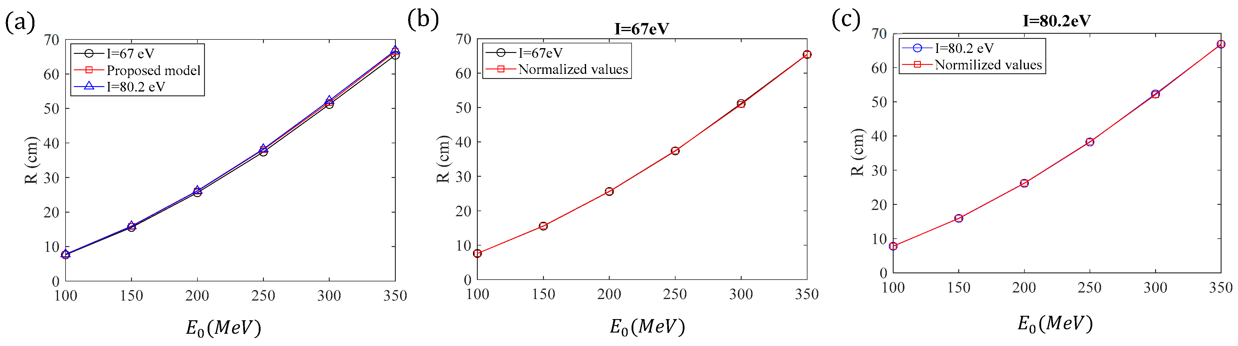
If considering $I=67 \mathrm{e}\mathrm{V}$, the exact range is slightly smaller than the one obtained using Equations (12), (16) and (17) and Table 3 (since these were derived by assuming $I=75 \mathrm{e}\mathrm{V}$). On the other hand, when using $I=80.2 \mathrm{e}\mathrm{V}$, the exact range is slightly larger than the one obtained using Equations (12), (16) and (17) and Table 3. The exact range for $I$= 67 eV and $I$ = 80.2 eV, along with the values derived by the model presented in this paper, are shown for comparison in Figure 6a. It is evident from Table 5 and Figure 6a that the errors related to the uncertainty of the ionization potential are small. In addition, it is straightforward to normalize the results concerning the range derived by the model proposed in this paper for the cases with ionization potentials of 67 eV and 80.2 eV. According to Table 5, the average error when $I=67 \mathrm{e}\mathrm{V}$ is 1.63% while the average error when $I=80.2 \mathrm{e}\mathrm{V}$ is 0.63%.

Therefore, for an ionization potential of 67 eV, we can normalize the model presented in this paper by reducing the values by 1.63%, and for an ionization potential of 80.2 eV, we can normalize them by increasing the values by 0.63%. In other words, for $I=67 \mathrm{e}\mathrm{V}$:

$$R_{I=67eV}=\left(1-{\displaystyle \frac{1.63}{100}}\right){\displaystyle \frac{\lambda }{\mu A}}\left(e^{\mu v_0}-1\right)$$

(23)

whereas, for $I=80.2 \mathrm{e}\mathrm{V}$:

$$R_{I=80.2eV}=\left(1+{\displaystyle \frac{0.63}{100}}\right){\displaystyle \frac{\lambda }{\mu A}}\left(e^{\mu v_0}-1\right)$$

(24)

The normalized values are presented in

Table 6. The exact range of protons for different initial energies is calculated considering $I=67 \mathrm{e}\mathrm{V}$ and $I=80.2 \mathrm{e}\mathrm{V}$. The results are compared with the normalized values based on the model proposed by this paper.

$\mathbf{Protons} \mathbf{(}\mathit{I} \mathbf{=} \mathbf{67} \mathbf{e}\mathbf{V}\mathbf{)}$
$\mathit{R}$ [Equation (18)]	${\mathit{R}}_{\mathit{n}\mathit{o}\mathit{r}\mathit{m}\mathbf{.}}$ (Equations (12), (16) and (17) and Table 3)	$\mathit{\pi } \mathbf{(}\mathbf{\%}\mathbf{)}$
7.60 cm	7.58 cm	0.26
15.54 cm	15.57 cm	0.19
25.58 cm	25.63 cm	0.20
37.39 cm	37.46 cm	0.19
51.15 cm	50.91 cm	0.47
65.41 cm	65.38 cm	0.05
Protons ($\mathit{I} \mathbf{=} \mathbf{80.2} \mathbf{e}\mathbf{V}$)
R (Equation (18))	${\mathit{R}}_{\mathit{n}\mathit{o}\mathit{r}\mathit{m}\mathbf{.}}$ (Equations (12), (16) and (17) and Table 3)	$\mathit{\pi } \mathbf{(}\mathbf{\%}\mathbf{)}$
7.78 cm	7.76 cm	0.25
15.91 cm	15.93 cm	0.13
26.17 cm	26.21 cm	0.15
38.23 cm	38.32 cm	0.24
52.27 cm	52.08 cm	0.36
66.82 cm	66.89 cm	0.10

and in Figure 6b,c.

Another critical issue, as already mentioned in the introduction, is the case of very small ranges, since these applications are related to new methods that combine radiotherapy with photodynamic therapy. In reference [15], proton energies between 15 MeV and 16 MeV were used, achieving a small penetration into matter of approximately 2 mm. For this case, we will repeat the procedure presented in Section 2. Since the initial energy range is small, we will consider constant $\mu$ and $\lambda$ values for initial energies between 15 MeV and 16 MeV. The exact values of the initial velocities, $R_{equiv.}$ and $\mu$, $\lambda$ parameters are presented in

Table 7. The calculation of the parameters $\mu$ and $\lambda$ for protons with initial energies of 15 MeV and 16 MeV (radiotherapy combined with PDT). The initial speed in these cases is also determined using Equation (2). The $f\left(v_0\right)$ value and the area under the $f\left(v\right)$ curve were used to determine $\mu , \lambda$. The calculations were performed considering $I=75 \mathrm{e}\mathrm{V}$ [20].

$\mathbf{Protons} \mathbf{(}\mathit{I} \mathbf{=} \mathbf{75} \mathbf{e}\mathbf{V}\mathbf{)}$
${\mathit{E}}_{\mathbf{0}} \mathbf{\left(}\mathbf{M}\mathbf{e}\mathbf{V}\mathbf{\right)}$	${\mathit{v}}_{\mathbf{0}}\mathbf{/}\mathit{c}$	${\mathit{v}}_{\mathbf{0}}\mathbf{/}{\mathbf{10}}^{\mathbf{8}} \mathbf{\left(}\mathbf{m}{\mathbf{s}}^{\mathbf{-}\mathbf{1}}\mathbf{\right)}$	$\frac{\mathit{f}\left({\mathit{v}}_{\mathbf{0}}\right)}{{\mathbf{10}}^{\mathbf{22}}} \mathbf{\left(}{\mathbf{m}}^{\mathbf{3}}{\mathbf{s}}^{\mathbf{-}\mathbf{3}}\mathbf{\right)}$	${\mathit{R}}_{\mathit{e}\mathit{q}\mathit{u}\mathit{i}\mathit{v}\mathbf{.}} \mathbf{\left(}\mathbf{m}\mathbf{m}\mathbf{\right)}$	${\mathit{\mu }}_{\mathit{P}\mathit{D}\mathit{T}}\mathbf{/}{\mathbf{10}}^{\mathbf{-}\mathbf{8}}$ $\mathbf{\left(}\mathbf{s}{\mathbf{m}}^{\mathbf{-}\mathbf{1}}\mathbf{\right)}$	${\mathit{\lambda }}_{\mathit{P}\mathit{D}\mathit{T}}\mathbf{/}{\mathbf{10}}^{\mathbf{20}}$$\mathbf{\left(}{\mathbf{m}}^{\mathbf{3}}{\mathbf{s}}^{\mathbf{-}\mathbf{3}}\mathbf{\right)}$
15	0.1767	0.5297	2.5750	2.52	6.5876	7.6695
16	0.1823	0.5466	2.8091	2.82	6.5876	7.6695

. This approximation yields excellent results, as shown in

Table 8. The proton’s range calculated using different methods in H₂O, considering $I=75 \mathrm{e}\mathrm{V}$ and initial energies of 15 MeV and 16 MeV. The model proposed by this paper leads to excellent results.

$$\mathbf{Range} \mathbf{Calculations}\mathbf{,} \mathbf{Protons} \mathbf{(}\mathit{I} \mathbf{=} \mathbf{75} \mathbf{e}\mathbf{V}\mathbf{)}$$
E (MeV)	$${\mathit{v}}_{\mathbf{0}}\mathbf{/}{\mathbf{10}}^{\mathbf{8}} \mathbf{\left(}\mathbf{m}{\mathbf{s}}^{\mathbf{-}\mathbf{1}}\mathbf{\right)}$$	R [Equation (7)]	R [Equation (18)]	R (Equation (12))
15	0.5297	2.52 mm	2.52 mm	2.52 mm
16	0.5466	2.82 mm	2.82 mm	2.82 mm

. Therefore, for applications that combine radiotherapy with photodynamic therapy (PDT) we can safely use the following values: ${\mu }_{PDT}=6.5876\times {10}^{-8} \mathrm{s}{\mathrm{m}}^{-1}$ and ${\lambda }_{PDT}=7.6695\times {10}^{20} {\mathrm{m}}^3{\mathrm{s}}^{-3}$.

The reason for repeating the procedure to calculate the appropriate μ and λ parameters is that Equations (16) and (17) were determined by fitting a polynomial function to the data in the range $100 \mathrm{M}\mathrm{e}\mathrm{V}\le E_0\le 250 \mathrm{M}\mathrm{e}\mathrm{V}$. For small initial energies, these equations are not applicable. For example, when using Equations (16) and (17) for $E_0=15 \mathrm{M}\mathrm{e}\mathrm{V}$, $\mu =4.4791\times {10}^{-8} \mathrm{s}{\mathrm{m}}^{-1}$ and $\lambda =-8.2759\times {10}^{20} {\mathrm{m}}^3{\mathrm{s}}^{-3}$. The negative value in the λ-parameter results in a negative range, which has no physical significance. In Figure 7, the functions $\mu =\mu \left(E_0\right)$ and $\lambda =\lambda \left(E_0\right)$, based on Equations (16) and (17), are presented in the range $15 \mathrm{M}\mathrm{e}\mathrm{V}\le E_0\le 250 \mathrm{M}\mathrm{e}\mathrm{V}$. The range of their applicability is also indicated ($100 \mathrm{M}\mathrm{e}\mathrm{V}\le E_0\le 250 \mathrm{M}\mathrm{e}\mathrm{V}$).

Another important point to address is how closely water represents tissue in terms of mean excitation potential. Water is often used as a surrogate for tissue due to its well-known properties, making it a reasonable approximation for soft tissue in many cases. However, it is important to acknowledge that tissues do vary in their composition and structure, which can lead to differences in their mean excitation potential compared to water. While water provides a good approximation for many soft tissues, particularly for general radiotherapy calculations, specific tissues like bone, fat, or muscle may have different mean excitation potentials. This variation can be important when high precision is required. In other words, the I-value is either overestimated or underestimated in many cases, depending on the tested tissue. Despite the fact that these errors are small, they may influence dose delivery, increasing the risk of radiation-induced side effects due to imperfect targeting of the tumor. This means there is a possibility of exposing surrounding healthy tissues to radiation.

Nonetheless, for most practical purposes, water remains a valid and widely accepted reference for the mean excitation potential in tissue modeling. Further discussions on this topic could indeed provide valuable insights, especially in contexts where tissue-specific properties are critical. Useful tables for the I-values of various biological materials are presented in [35].

It is also important to note that the use of Monte Carlo simulations leads to a more accurate solution compared to the numerical integration of the Bethe equation. This is because Monte Carlo simulations can account for proton-nucleus scattering events that the Bethe equation does not consider. For these reasons, small deviations in range calculations may arise when using our model compared to Monte Carlo simulations or real experiments. However, for a Monte Carlo solution to be truly effective, it requires an acceptable definition of the Monte Carlo range, as well as a deep understanding of the Monte Carlo method and the nuances of setting all necessary parameters. On the other hand, the proposed approach, based on solving the Bethe equation, provides valuable insights into the physical behavior of the system, particularly given the complexities associated with achieving a professional and realistic Monte Carlo solution. Therefore, despite not providing the ‘exact’ solution, the error is minor, and the method is extremely simple and easily applicable by practitioners in radiotherapy.

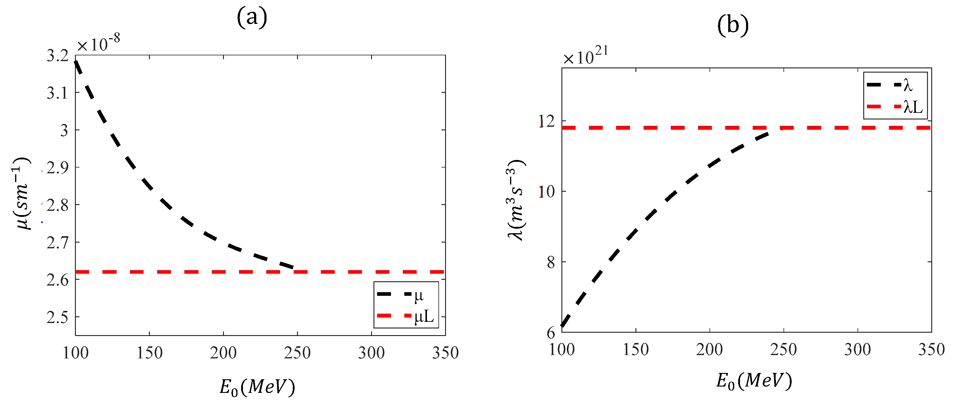
In addition, an interesting question that arises is why polynomial fittings were used for the $\mu$ and $\lambda$ parameters, as described in Equations (16) and (17). Given the approximation of a limiting value for energies greater than 250 MeV, a more rational approach would be to invoke exponential functions combined with a constant term in both cases. The reason for not employing the latter approach is that only third-degree polynomials provided a perfect fit to the data within the range of 100 MeV to 250 MeV. The errors if using exponential fits would be larger than the ones presented in Section 2 and Section 3. Therefore, using the approach presented in this paper, we successfully achieved precise and straightforward solutions for determining the range of protons in a medium. Additionally, it is important to note that this paper focused on protons traveling through a medium across the entire range of energies relevant to biomedical applications. The same methods can also be applied to other charged particles, such as carbon ions [36]. For the case of carbon ions, the atomic number z is 6, and the particle’s mass is $m_p=2.007\times {10}^{-26} \mathrm{k}\mathrm{g}$ [20]. Therefore, the parameter A in Equation (3) is equal to: $A=4.4013\times {10}^{32} {\mathrm{m}}^3{\mathrm{s}}^{-4}$. To further test the model proposed in this paper, we present

Table 9. The range of carbon ions was calculated using Equation (12), considering I = 75 eV and various initial energies. The results from the model proposed in this paper (Equation (12)) are compared with experimental results and results from the PSTAR database presented in [20,37,38,39]. In all cases, the errors are low. ${\pi }_1$ (%) indicates the percentage differences between the experimental results and the results from Equation (12), while ${\pi }_2$ (%) represents the differences between Equation (12) and the PSTAR database.

$\mathbf{Carbon} \mathbf{Ions} \mathbf{(}\mathit{I} \mathbf{=} \mathbf{75} \mathbf{e}\mathbf{V}\mathbf{)}$
${\mathit{E}}_{\mathbf{0}} \mathbf{\left(}\mathbf{M}\mathbf{e}\mathbf{V}\mathbf{\right)}$	${\mathit{v}}_{\mathbf{0}}\mathbf{/}{\mathbf{10}}^{\mathbf{8}} \mathbf{(}\mathbf{m}\mathbf{/}\mathbf{s}\mathbf{)}$	$\mathit{\mu }\mathbf{/}{\mathbf{10}}^{\mathbf{-}\mathbf{8}}$ $\mathbf{\left(}\mathbf{s}{\mathbf{m}}^{\mathbf{-}\mathbf{1}}\mathbf{\right)}$	$\mathit{\lambda }\mathbf{/}{\mathbf{10}}^{\mathbf{22}}$ $\mathbf{\left(}{\mathbf{m}}^{\mathbf{3}}{\mathbf{s}}^{\mathbf{-}\mathbf{3}}\mathbf{\right)}$	R (cm) (Equation (12))	R (cm) (Exper.)	R (cm) (PSTAR) [20]	${\mathit{\pi }}_{\mathbf{1}}$ (%)	${\mathit{\pi }}_{\mathbf{2}}$ (%)
135.00	1.4554	2.9242	0.8163	4.41	4.43 [37]	4.37	0.45	0.91
195.00	1.6811	2.7073	1.0574	8.32	8.34 [37]	8.28	0.24	0.48
241.50	1.8172	2.6387	1.1669	12.05	11.87 [38]	11.92	1.50	1.08
270.00	1.8887	2.6200	1.1800	14.32	14.45 [38]	14.37	0.90	0.35
279.97	1.9119	2.6200	1.1800	15.22	14.73 [39]	15.27	3.23	0.33
330.00	2.0169	2.6200	1.1800	20.08	19.98 [37]	20.04	0.50	0.20
332.15	2.0210	2.6200	1.1800	20.30	19.74 [39]	20.25	2.76	0.25
380.45	2.1064	2.6200	1.1800	25.41	24.76 [39]	25.25	2.56	0.63

, which compares range calculations in H₂O for carbon ions with experimental results and results for the PSTAR database.

Future research will focus on further experimental validation in clinical settings, such as proton therapy centers. Since the model proposed in this paper has been proven to be accurate, simple, and free from computational demands or high processing times, it is likely to become a valuable tool in real clinical applications.

5. Conclusions

This paper presented a straightforward approach for monitoring protons within a medium for biomedical applications. Despite the availability of mathematical models designed to simplify computational processes with high computational demands, these models often require advanced mathematical and physical expertise or are limited to scenarios where relativistic effects are small. Therefore, in this paper, we provided straightforward equations that can be easily applied by practitioners without a strong mathematical background. The simplification of the mathematical processes is based on Equation (9), where a simple exponential alternative to the function $f\left(v\right)$ was derived using fitting procedures. By utilizing this exponential parameter, calculating the proton range and solving Berthe’s equations become straightforward tasks. The key findings of this paper can be summarized as follows:

▪

For conventional cases (initial energies of protons between 100 MeV and 250 MeV), the range of the protons within a medium can be easily determined using Equations (12), (16) and (17).

▪

For high initial energies (up to 350 MeV), the parameters $\mu$ and $\lambda$ can be approximated by the limiting values presented in Table 3.

▪

For very low energies (focused on combining radiotherapy with PDT), the $\mu$ and $\lambda$ values from Table 7 should be used instead.

▪

In any case, the solution of the Bethe equation (i.e., the function $v=f\left(x\right)$) can be approximated by Equation (22). Equation (22) leads to accurate results even for high proton energies with very large ranges within a medium.

▪

From a purely mathematical and physical perspective, the procedures shown in Section 2, Section 3 and Section 4 can be used to find the range and functions $v=f\left(x\right)$ of any charged particle for any energy (even for $E_0>350 \mathrm{M}\mathrm{e}\mathrm{V}$).

▪

The model presented in this paper uses an ionization potential of $I=75 \mathrm{e}\mathrm{V}$. Other values presented in the literature are $I=67 \mathrm{e}\mathrm{V}$ and $I=80.2 \mathrm{e}\mathrm{V}$. It was shown that the exact value of the ionization potential leads to small errors (between 0.40% and 1.87%). These errors can be minimized with normalization factors, as explained in the Discussion section (Equations (23) and (24)).

In conclusion, this paper presents a straightforward method for monitoring charged particles in a medium for biomedical applications. The proposed approach has three main points demonstrating its practical applicability. First, unlike Monte Carlo simulations, which require highly skilled personnel, our method simplifies the process with elementary solutions for the range and v(x) functions. Second, the analytical form is computationally efficient, making it ideal for optimization scenarios with multiple iterations of dose calculations. In addition, typical Monte Carlo simulations can take a non-negligible amount of time (from several minutes to several hours per patient). Therefore, our proposed method is significantly more efficient. Third, while existing solutions to the Bethe equation require advanced skills or are limited to small initial energies, our equations are simple, applicable to both small and large energies, and easy for non-experts to use. These factors suggest that the equations presented could be a valuable tool in radiotherapy.

References

1. Chong, L.M.; Tng, D.J.H.; Tan, L.L.Y.; Chua, M.L.K.; Zhang, Y. Recent advances in radiation therapy and photodynamic therapy. Appl. Phys. Rev. 2021, 8, 041322. [Google Scholar] [CrossRef]
2. Ferlay, J.; Colombet, M.; Soerjomataram, I.; Mathers, C.; Parkin, D.M.; Piñeros, M.; Znaor, A.; Bray, F. Estimating the global cancer incidence and mortality in 2018: GLOBOCAN sources and methods. Cancer Epidemiol. 2019, 144, 1941–1953. [Google Scholar] [CrossRef] [PubMed]
3. Ahmad, S.S.; Duke, S.; Jena, R.; Williams, M.V.; Burnet, N.G. Advances in radiotherapy. BMJ 2012, 345, e7765. [Google Scholar] [CrossRef] [PubMed]
4. Ragoowansi, R.; Comes, P.G.S.; Moss, A.L.; Glees, J.P. Treatment of keloids by surgical excision and immediate postoperative single-fraction radiotherapy. Plast. Reconstr. Surg. 2003, 111, 1853–1859. [Google Scholar] [CrossRef]
5. Godfrey, K.J.; Kazim, M. Radiotherapy for active thyroid eye disease. Ophthalmic Plast. Reconstr. Surg. 2018, 34, S98–S104. [Google Scholar] [CrossRef]
6. Al-Mamgani, A.; Heemsbergen, W.D.; Peeters, S.T.H.; Lebesque, J.V. Role of intensity-modulated radiotherapy in reducing toxicity in dose escalation for localized prostate cancer. Int. J. Radiat. Oncol. Biol. Phys. 2009, 73, 685–691. [Google Scholar] [CrossRef]
7. Konski, A. Radiotherapy is a cost-effective palliative treatment for patients with bone metastasis from prostate cancer. Int. J. Radiat. Oncol. Biol. Phys. 2004, 60, 1373–1378. [Google Scholar] [CrossRef]
8. Creutzberg, C.L.; van Putten, W.L.; Koper, P.C.; Lybeert, M.L.; Jobsen, J.J.; Wárlám-Rodenhuis, C.C.; De Winter, K.A.; Lutgens, L.C.; van den Bergh, A.C.; van de Steen-Banasik, E.; et al. Surgery and postoperative radiotherapy versus surgery alone for patients with stage-1 endometrial carcinoma: Multicentre randomised trial. Lancet 2000, 355, 1404–1411. [Google Scholar] [CrossRef]
9. Holt, A.; van Vliet-Vroegindeweij, C.; Mans, A.; Belderbos, J.S.; Damen, E.M.F. Volumetric-modulated arc therapy for stereotactic body radiotherapy of lung tumors: A comparison with intensity-modulated radiotherapy techniques. Int. J. Radiat. Oncol. Biol. Phys. 2011, 81, 1560–1567. [Google Scholar] [CrossRef]
10. Schuitmaker, J.J.; Baas, P.; van Leengoed, H.L.L.M.; van der Meulen, F.W.; Star, W.M.; van Zandwijk, N. Photodynamic therapy: A promising new modality for the treatment of cancer. J. Photochem. Photobiol. B Biol. 1996, 34, 3–12. [Google Scholar] [CrossRef]
11. Kübler, A.C. Photodynamic therapy. Med. Laser Appl. 2005, 20, 37–45. [Google Scholar] [CrossRef]
12. Mitra, A.; Stables, G.I. Topical photodynamic therapy for non-cancerous skin conditions. Photodiagnosis Photodyn. Ther. 2006, 3, 116–127. [Google Scholar] [CrossRef]
13. Alexiades-Armenakas, M. Laser-mediated photodynamic therapy. Clin. Dermatol. 2006, 24, 16–25. [Google Scholar] [CrossRef] [PubMed]
14. Sun, W.; Luo, L.; Feng, Y.; Cai, Y.; Zhuang, Y.; Xie, R.-J.; Chen, X.; Chen, H. Aggregation-induced emission gold clustoluminogens for enhanced low-dose X-ray-induced photodynamic therapy. J. Am. Chem. Soc. 2020, 132, 10000–10007. [Google Scholar]
15. Grigalavicius, M.; Mastrangelopoulou, M.; Berg, K.; Arous, D.; Ménard, M.; Raabe-Henriksen, T.; Brondz, E.; Siem, S.; Görgen, A.; Edin, N.F.J.; et al. Proton-dynamic therapy following photosensitizer activation by accelerated protons demonstrated through fluorescence and singlet oxygen production. Nat. Commun. 2019, 10, 3986. [Google Scholar] [CrossRef]
16. Paganetti, H. Range uncertainties in proton therapy and the role of Monte Carlo simulations. Phys. Med. Biol. 2012, 57, R99–R117. [Google Scholar] [CrossRef]
17. Agostinelli, S.; Allison, J.; Amako, K.; Apostolakis, J.; Araujo, H.; Arce, P.; Asai, M.; Axen, D.; Banerjee, S.; Barrand, G.; et al. Geant4—A simulation toolkit. Nucl. Instrum. Methods Phys. Res. A 2003, 506, 250–303. [Google Scholar] [CrossRef]
18. Pelowitz, D.B.; Durkee, J.W.; Elson, J.S.; Fensin, M.L.; Hendricks, J.S.; James, M.R.; Johns, R.C.; McKinney, G.W.; Mashnik, S.G.; Verbeke, J.M.; et al. MCNPX 2.7.0 Extensions; Los Alamos National Laboratory (LANL): Los Alamos, NM, USA, 2011. [Google Scholar]
19. Ferrari, A.; Sala, P.R.; Fasso, A.; Ranft, J. FLUKA: A Multi-Particle Transport Code (Program Version 2005); CERN Yellow Reports: Monographs; CERN (GENEVA): Geneva, Switzerland, 2005. [Google Scholar]
20. Grimes, D.R.; Warren, D.R.; Partridge, M. An approximate analytical solution of the Bethe equation for charged particles in the radiotherapeutic energy range. Sci. Rep. 2017, 7, 9781. [Google Scholar] [CrossRef]
21. Martinez, D.M.; Rahmani, M.; Burbadge, C.; Hoehr, C. A practical solution of the Bethe equation in the energy range applicable to radiotherapy and radionuclide production. Sci. Rep. 2019, 9, 17599. [Google Scholar] [CrossRef]
22. Echeweozo, E.O.; Abdelmonem, A.M. Evaluation of interaction properties of some ionizing radiation with selected nitrogen-based explosives. Arab J. Sci. Eng. 2024, 49, 1025–1036. [Google Scholar] [CrossRef]
23. Abdelmonem, A.M.; Echeweozo, E.O. Investigation of interaction parameters of gamma radiation, neutron, and charge particles in selected thermoplastic polymers for radiation protection. J. Mater. Sci. Mater. Electron. 2023, 34, 365. [Google Scholar] [CrossRef]
24. Rahmani, M.; Martinez, D.M. Convection driven by a nonuniform radiative internal heat source in a cavity: Example of medical isotope production in liquid targets. Int. J. Heat Mass Transf. 2024, 231, 125872. [Google Scholar] [CrossRef]
25. Berger, M.; Coursey, J.; Zucker, M.; Chang, J. Estar, Pstar, and Astar: Computer Programs for Calculating Stopping-Power and Range Tables for Electrons, Protons, and Helium Ions (Version 1.2.3); National Institute of Standards and Technology: Gaithersburg, MD, USA, 2005. [Google Scholar]
26. Lu, X.; Li, Z.; Dolgashev, V.; Bowden, G.; Sy, A.; Tantawi, S.; Nanni, E.A. A proton beam energy modulator for rapid proton therapy. Rev. Sci. Instrum. 2021, 92, 024705. [Google Scholar] [CrossRef] [PubMed]
27. Li, W.G.; Chang, C.; Qin, Y.; Wang, Z.-L.; Li, K.-W.; Geng, L.-S.; Wu, H. GPU-based cross-platform Monte Carlo proton dose calculation engine in the framework of Taichi. Nucl. Sci. Tech. 2023, 34, 77. [Google Scholar] [CrossRef]
28. Kontomaris, S.V.; Mazi, I.; Chliveros, G.; Malamou, A. Generic numerical and analytical methods for solving nonlinear oscillators. Phys. Scr. 2024, 99, 025231. [Google Scholar] [CrossRef]
29. He, J.H. The simplest approach to nonlinear oscillators. Results Phys. 2019, 15, 102546. [Google Scholar] [CrossRef]
30. He, J.H. Frequency formulation for nonlinear oscillators (part 1). Sound Vib. 2024, 59, 1687. [Google Scholar] [CrossRef]
31. Cveticanin, L.; Zukovic, M.; Cveticanin, D. Approximate analytic frequency of strong nonlinear oscillator. Mathematics 2024, 12, 3040. [Google Scholar] [CrossRef]
32. Schinner, P.; Bimbot, R.; Geissel, H.; Paul, H.; Schinner, A. Sigmund. Stopping of ions heavier than helium. J. ICRU 2005, 5. Available online: https://portal.findresearcher.sdu.dk/en/publications/stopping-of-ions-heavier-than-helium (accessed on 25 March 2025).
33. Powers, S. Stopping powers and ranges for protons and alpha particles. In ICRU Report 49; International Commission on Radiation Units and Measurements: Bethesda, MD, USA, 2005. [Google Scholar]
34. Paul, H. The mean ionization potential of water, and its connection to the range of energetic carbon ions in water. Nucl. Instrum. Methods Phys. Res. B 2007, 255, 435–437. [Google Scholar] [CrossRef]
35. Bär, E.; Andreo, P.; Lalonde, A.; Royle, G.; Bouchard, H. Optimized I-values for use with the Bragg additivity rule and their impact on proton stopping power and range uncertainty. Phys. Med. Biol. 2018, 63, 165007. [Google Scholar] [CrossRef] [PubMed]
36. Nascimento, L.d.F.; De Saint-Hubert, M.; Caprioli, M.; Delombaerde, L.; Himschoot, K.; Vandenbroucke, D.; Leblans, P.; Crijns, W.; Kodaira, S. Characterization of a real-time dosimetry system using 2D nano and micro-coatings in proton and carbon therapeutic ion beams. Radiat. Meas. 2024, 178, 107303. [Google Scholar] [CrossRef]
37. Sihver, L.; Schardt, D.; Kanai, T. Depth-Dose Distributions of High-Energy Carbon, Oxygen and Neon Beams in Water. J. Med. Phys. 1998, 18, 1–21. [Google Scholar]
38. Yamamoto, S.; Komori, M.; Koyama, S.; Toshito, T. Luminescence Imaging of Water During Alpha Particle Irradiation. Nucl. Instrum. Methods Phys. Res. Sect. A 2016, 819, 6–13. [Google Scholar] [CrossRef]
39. Farina, E.; Piersimoni, P.; Riccardi, C.; Rimoldi, A.; Tamborini, A.; Ciocca, M. Geant4 Simulation for a Study of a Possible Use of Carbon Ion Pencil Beams for the Treatment of Ocular Melanomas with the Active Scanning System at CNAO. J. Phys. Conf. Ser. 2015, 664, 072048. [Google Scholar] [CrossRef]
Figure 1. (ad) The exponential approximation of Equation (9) is presented graphically. Blue curves represent the actual f ( v ) data, while the red dotted lines represent the exponential approximation for (a) 0 v / c 0.4281 ( 0 E 100   M e V ), (b) 0 v / c 0.5066 ( 0 E 150   M e V ), (c) 0 v / c 0.5661 ( 0 E 200   M e V ) and (d) 0 v / c 0.6135 ( 0 E 250   M e V ). The values of μ and λ for the exponential curves in (ad) are the ones presented in Table 1. (e) μ with respect to E 0 data and the polynomial fit (Equation (16)). (f) λ with respect to E 0 data and the polynomial fit (Equation (17)).
Sci 07 00049 g001
Figure 2. (a) The proposed method involves considering an equivalent exponential function that has the same area under the curve and the same maximum value as the actual f function. (b) The system of equations used for the determination of μ and λ for a given initial speed. (c) Using fitting procedures, the μ = μ ( E 0 ) and λ = λ ( E 0 ) functions were determined.
Sci 07 00049 g002
Figure 3. The functions v = f ( x ) for different initial energies of protons in H2O considering I = 75   e V .
Sci 07 00049 g003
Figure 4. The (a) μ = μ ( E 0 ) and (b) λ = λ ( E 0 ) graphs when using Equations (16) and (17) along with the limiting values μ L and λ L , respectively.
Sci 07 00049 g004
Figure 5. The v = f ( x ) functions for different initial energies of protons in H2O for I = 75   e V . The initial energies are (a) 300 MeV and (b) 350 MeV.
Sci 07 00049 g005
Figure 6. (a) The range values derived in this model, where it was assumed that the ionization potential is 75 eV. These values are compared to the exact range values, which were calculated numerically using Equation (18) for I = 67   e V and I = 80.2   e V . For the first case, there is an average error of 1.63% (the model presented in this paper overestimates the range), whereas for the latter case there is an average error of 0.63% (the model presented in this paper underestimates the range). (b) For I = 67   e V , the values derived by the proposed model can be normalized by an average decrease of 1.63%. In this case, the exact results and the normalized results are nearly identical. (c) For I = 80.2   e V , the values derived by the proposed model can be normalized by an average increase of 0.63%. Using this approach, the exact results and the normalized results are nearly identical.
Sci 07 00049 g006
Figure 7. (a) The μ = μ ( Ε 0 ) and the (b) λ = λ ( Ε 0 ) functions in the domain 15   M e V E 0 250   M e V . Equations (16) and (17) can only be used for E 0 100   M e V .
Sci 07 00049 g007