Article

On Hens, Eggs, Temperatures and CO2: Causal Links in Earth’s Atmosphere

by
Demetris Koutsoyiannis
1,*,
Christian Onof
2,
Zbigniew W. Kundzewicz
3 and
Antonis Christofides
1
1
Department of Water Resources and Environmental Engineering, School of Civil Engineering, National Technical University of Athens, 15778 Zographou, Greece
2
Department of Civil and Environmental Engineering, Faculty of Engineering, Imperial College London, London SW7 2BX, UK
3
Meteorology Lab, Department of Construction and Geoengineering, Faculty of Environmental Engineering and Mechanical Engineering, Poznan University of Life Sciences, 60-637 Poznań, Poland
*
Author to whom correspondence should be addressed.
Submission received: 17 March 2023 / Revised: 24 May 2023 / Accepted: 5 September 2023 / Published: 13 September 2023
(This article belongs to the Special Issue Feature Papers—Multidisciplinary Sciences 2023)

Abstract

:
The scientific and wider interest in the relationship between atmospheric temperature (T) and concentration of carbon dioxide ([CO2]) has been enormous. According to the commonly assumed causality link, increased [CO2] causes a rise in T. However, recent developments cast doubts on this assumption by showing that this relationship is of the hen-or-egg type, or even unidirectional but opposite in direction to the commonly assumed one. These developments include an advanced theoretical framework for testing causality based on the stochastic evaluation of a potentially causal link between two processes via the notion of the impulse response function. Using, on the one hand, this framework and further expanding it and, on the other hand, the longest available modern time series of globally averaged T and [CO2], we shed light on the potential causality between these two processes. All evidence resulting from the analyses suggests a unidirectional, potentially causal link with T as the cause and [CO2] as the effect. That link is not represented in climate models, whose outputs are also examined using the same framework, resulting in a link opposite the one found when the real measurements are used.

Graphical Abstract

Science is generated by and devoted to free inquiry: the idea that any hypothesis, no matter how strange, deserves to be considered on its merits. The suppression of uncomfortable ideas may be common in religion and politics, but it is not the path to knowledge; it has no place in the endeavor of science. We do not know in advance who will discover fundamental new insights.
Carl Sagan [1]

1. Introduction

A recent (2020) study [2] examining data from measurements of temperature (T) and atmospheric concentration of carbon dioxide ([CO2]) challenged the conventional, and well established, wisdom that increased [CO2] causes an increase in temperature. The study examined whether the commonly assumed causal chain is supported by data or, alternatively, whether a hen-or-egg (HOE) causal relationship is more plausible. The phrase “hen or egg” (originally in Greek, ὄρνις ἢ ᾠὸν) was first used in a philosophical context by Plutarch [3] to describe situations in which it is not clear which of two interrelated events or processes is the cause and which the effect.
The study examined a case where the causal link is not between two events but between two processes, represented as stochastic processes. Denoting these processes as x _ t and y _ t (where we follow the Dutch notational convention of underlining stochastic variables), in a typical causal system, denoted as x y , earlier realizations of x _ t affect the current realization of y _ t . In an HOE causal system, earlier realizations of x _ t affect the current realization of y _ t , but also earlier realizations of y _ t affect the current realization of x _ t .
In terms of its applications, the study used global temperature data from satellites (University of Alabama in Huntsville—UAH) and ground-based (CRUTEM.4.6.0.0 global T 2 m land temperature) and [CO2] data at several sites (Mauna Loa, HI, USA; Barrow, AK, USA; South Pole; global average) with monthly time steps for the period 1980–2019. An innovative element of this study was that it explained the reasons why using the original T and [CO2] data series yielded spurious results, and it proposed using the changes (differences in time) thereof instead. We note that differencing is of very common use in economics literature (e.g., [4,5]). In particular, for the [CO2] it proposed taking the logarithm before differencing (something resembling techniques used in economics [5]) and thus the time series that were correlated were Δ T and Δ l n [ C O 2 ] , where the differences are taken over 12 months. By studying lagged correlations of the two, the study asserted that, while both causality directions exist, the results support the hypothesis that the dominant direction is T → CO2. Changes in [CO2] follow changes in T by about six months on a monthly scale or about one year on an annual scale. In turn, the study attempted to interpret this mechanism by referring to biochemical reactions, since at higher temperatures soil respiration, and hence CO2 emission, increases.
In a subsequent (2022) two-paper study, Koutsoyiannis et al. [6,7] developed a more complete theoretical framework by revisiting causality over the entire knowledge tree, from philosophy to science and to scientific and technological application. By reviewing various approaches to causality, the study located several problems in identifying causal links. Hence, the study developed the theoretical background of a stochastic approach to causality, with the objective of formulating necessary conditions that are operationally useful in identifying or falsifying causality claims. It also developed an effective algorithm applicable to large-scale open systems, which are neither controllable nor repeatable. The proposed framework was illustrated and showcased in a number of case studies, some of which were controlled synthetic examples and others real-world ones arising from interesting scientific problems in geophysics and, in particular, hydrology and climatology. The relationship of globally averaged temperature with [CO2] concentration (again in terms of differences Δ T and Δ l n [ C O 2 ] over 12 months) was included in the thirty case studies presented. In brief, the related analyses pointed to the following (quoting from [7]):
Clearly, the results […] suggest a (mono-directional) potentially causal system with T as the cause and [CO2] as the effect. Hence the common perception that increasing [CO2] causes increased T can be excluded as it violates the necessary condition for this causality direction.
[…] in other words, it is the increase of temperature that caused increased CO2 concentration. Though this conclusion may sound counterintuitive at first glance, because it contradicts common perception […], in fact it is reasonable. The temperature increase began at the end of the Little Ice Period, in the early nineteenth century, when human CO2 emissions were negligible […].
However, the scope of that study [6,7] was to formulate a general methodology for the detection of causality—in particular, necessary conditions thereof—rather than to study a specific system in detail. Therefore, no detailed modeling was made in the case studies, including the hydrological and climatic applications. However, given the enormous interest in the T-[CO2] relationship, here we will go deeper into this.
Specifically, this paper, after summarizing the methodology (Section 2) and the data used (Section 3), focuses on the latter relationship with the following objectives:
  • To expand the time frame of the investigation backward and forward by exploiting the longest available data series (Section 4).
  • To check whether seasonality, as reflected in different phases of [CO2] time series at different latitudes, plays any role that could modify or possibly reverse the detected causality relationship (Section 5).
  • To propose and apply a method for investigating the effect of the timescale in causality detection (Section 6).
  • To extend the methodology for disambiguating cases in which the type of causality, HOE or unidirectional, is not quite clear (Section 7).
  • To exploit the methodology in defining a type of data analysis that, regardless of the detection of causality per se, could shed light on modeling performance by comparing observational data with model results (Section 8).
  • To discuss possible extensions of the scope of the methodology, i.e., from detecting possible causality to building a more detailed model of stochastic type (Section 9).
  • To provide logical support for the findings by revisiting the carbon balance in the atmosphere (Appendix A.1) and investigating additional processes that may have caused increases in temperature (Appendix A.2, Appendix A.3 and Appendix A.4).

2. Summary of the Stochastic Approach to Causality
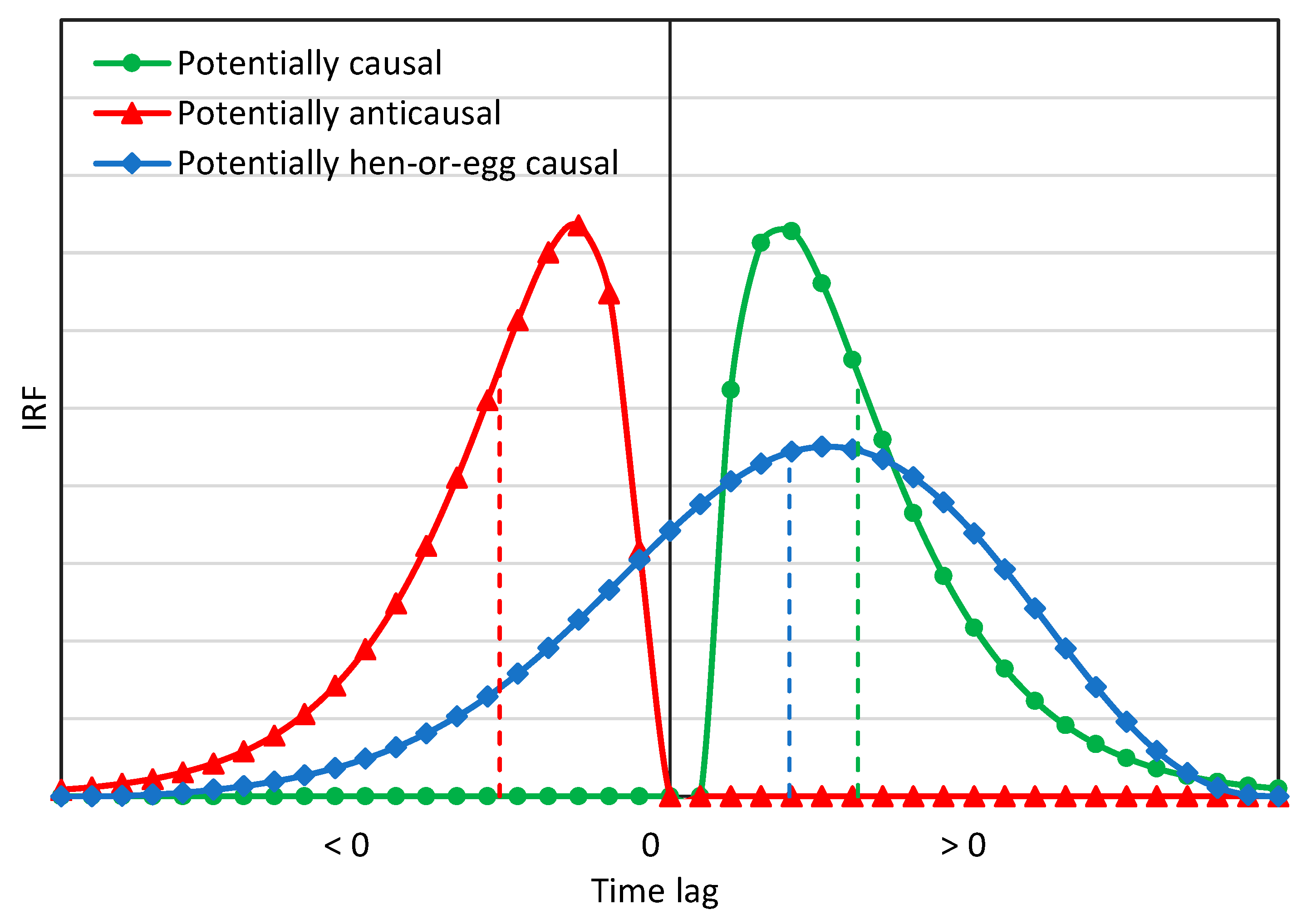
The methodology in [6,7] is based on the impulse response function (IRF) between two processes x _ ( t ) ,   y _ ( t ) , denoted as g ( h ) where h denotes time lag, based on the convolution
y _ t = g ( h ) x _ ( t h ) d h + v _ ( t )
where v _ ( t ) is another stochastic process representing the part that is not explained by the causal link. To see that the function g ( h ) is the impulse response function (IRF) of the system ( x _ t , y _ t ), we set v _ t 0 and x _ t = δ ( t ) (the Dirac delta function, representing an impulse of infinite amplitude at t = 0 and attaining the value of 0 for t 0 ), and we readily get y _ t = g ( t ) .
On the other hand, if we set g h = b   δ ( h h 0 ) (with constant b and h 0 ), which means that the IRF is zero for every lag except for the specific lag h 0 , then Equation (1) becomes y _ t = b x _ t h 0 + v _ ( t ) . This special case is equivalent to simply correlating y _ t with x _ t h 0 at any time instance t . It is easy to find (cf. linear regression) that in this case the multiplicative constant b is the correlation coefficient of y _ t and x _ t h 0 multiplied by the ratio of the standard deviations of the two processes. In general, however, we expect that the actual g ( h ) is not a Dirac delta function but a continuous one over some domain. Thus, the IRF is a much more powerful tool than correlation as it integrates the correlations in the entire spectrum of lags.
For any two processes x _ ( t ) and y _ t , Equation (1) has infinitely many solutions in terms of the function g h and the process v _ ( t ) . An obvious and trivial one is g h 0 , y _ t v _ ( t ) . The sought solution is the one that corresponds to the minimum variance of v _ ( t ) , called the least-squares solution. Equivalently, this solution maximizes the explained variance ratio:
e   : = 1   γ υ   γ y
where   γ υ and   γ y denote the variances of the processes v _ ( t ) and y _ t , respectively. (This is similar as in the correlation at a single time lag.) If the attained maximum e is close to zero, this will mean that the two processes are uncorrelated and thus no causality condition can exist between them (a non-causal system).
Otherwise, we may assume, without loss of generality, that processes x _ ( t ) and y _ t are positively correlated (i.e., an increase in x _ ( t ) would result in an increase in y _ t ). In the opposite case (if the processes are negatively correlated), by multiplying one of the two series by 1 we make the correlation positive. Therefore, we impose a nonnegativity constraint for the sought IRF,
g h 0
In the estimation of IRF, we may also impose a roughness constraint,
E E 0
where E is the roughness of the IRF determined in terms of the second derivative of g ( h ) :
Ε   : = g h 2 d h
Further justification for the two constraints is provided in [6].
In applications, the continuous time representation is replaced by a discrete time one, the IRF becomes a sequence of values g j , where j denotes the time lag, the infinite range of the time lag h becomes a finite window of time lag j , specified in the interval [ J , J ] , the integrals are replaced by sums, and the true values of statistics are replaced by estimates. Furthermore, the roughness E is standardized as
ε   : = E 8 j = J J g j 2
where ε ranges in (0,1) for nonnegative g j . The determination of the IRF ordinates g j is thus formulated as a constrained optimization problem, whose numerical solution is always possible, simple and fast, and can be attained even by commonly available solvers, e.g., in commercial or open source spreadsheet software.
We note that in applications, each of the directions x y and y x is investigated separately, as there is no symmetry (or antisymmetry) in the produced IRFs in the two directions. When we refer to direction y x we mean that we interchange the time series x and y and still estimate the IRF in the same way, as described in our equations in which the direction x y is assumed.
In applications investigating causality, we start by assuming a potentially hen-or-egg (HOE) causal model with a fixed number of weights g j ,   j = J , , 0 , J , where in most of the cases studied in [7] the value J = 20 was adopted, and this is also followed here. Depending on the results of the estimation procedure, if e is non-negligible, the system is deemed:
  • Potentially HOE causal if we have g j > 0 for both some positive and some negative lags j,
  • Potentially causal if g j = 0 for all j < 0 , and
  • Potentially anticausal if g j = 0 for all j > 0
Note that anticausal means that the actual causality direction is opposite to that assumed. These three cases are graphically illustrated in Figure 1. The adverb “potentially” in the above characterizations highlights the fact that the conditions tested provide necessary but not sufficient conditions for causality.
In a potentially causal (or anticausal) system, the time order is explicitly reflected in the above characterizations. In a potentially HOE causal system, the time order needs to be clarified by defining the principal direction. The most natural indices for this are: (a) the time lag h c maximizing the absolute value of cross-covariance; (b) the mean (time average) μ h of the function   g ( h ) ; and (c) the median h 1 / 2 of the function   g ( h ) . We note that h c , which was the basis in the original study [2], is completely independent from the g ( h ) . The other two, μ h and h 1 / 2 , depend on the g ( h ) that is determined. However, extensive analyses in [7] showed that their estimation is quite robust; for example, the use of the roughness constraint, while affecting the resulting g ( h ) , practically does not affect the values of μ h and h 1 / 2 . In general, the characteristic lags μ h and h 1 / 2 do not differ substantially from each other, and any of them could be chosen for further use. Here we prefer to note both, as well as h c , as they all provide useful information about the relationship of the two processes (like in the case of using both mean and median in the characterization of the probability distribution of a single variable).
Needless to say, the literature offers a spectrum of alternative methods for estimating an IRF, using different tools such as auto- and cross-correlations functions [8,9], power spectra and cross-spectra based on the Fourier transform [10] or on a wavelet transform [11], as well as principal component analysis [12]. The method described above has some advantages over these alternatives, as it is a direct method that can work with time series of observations per se, rather than transformations thereof, being easily understandable and reproducible by any reader using simple computational means. Additionally, it is more reliable as it avoids using uncertain estimates of autocorrelation functions or their more uncertain transformations, such as the power spectrum, i.e., the Fourier transform of the autocorrelation function. Note that here we also used autocorrelation, but only to validate and confirm our results—not in the estimation procedure.
Additionally, as detailed in [6], our method differs conceptually and computationally from the so-called “Granger causality” [13,14] (a misnomer, as the method does not infer causality but prediction) and more recently reformulated in the study of Moraffah et al. [15], which also discusses other similar methods. Finally, our method has substantial differences from a framework proposed by Pearl and collaborators [16,17,18] as again discussed in detail in [6].

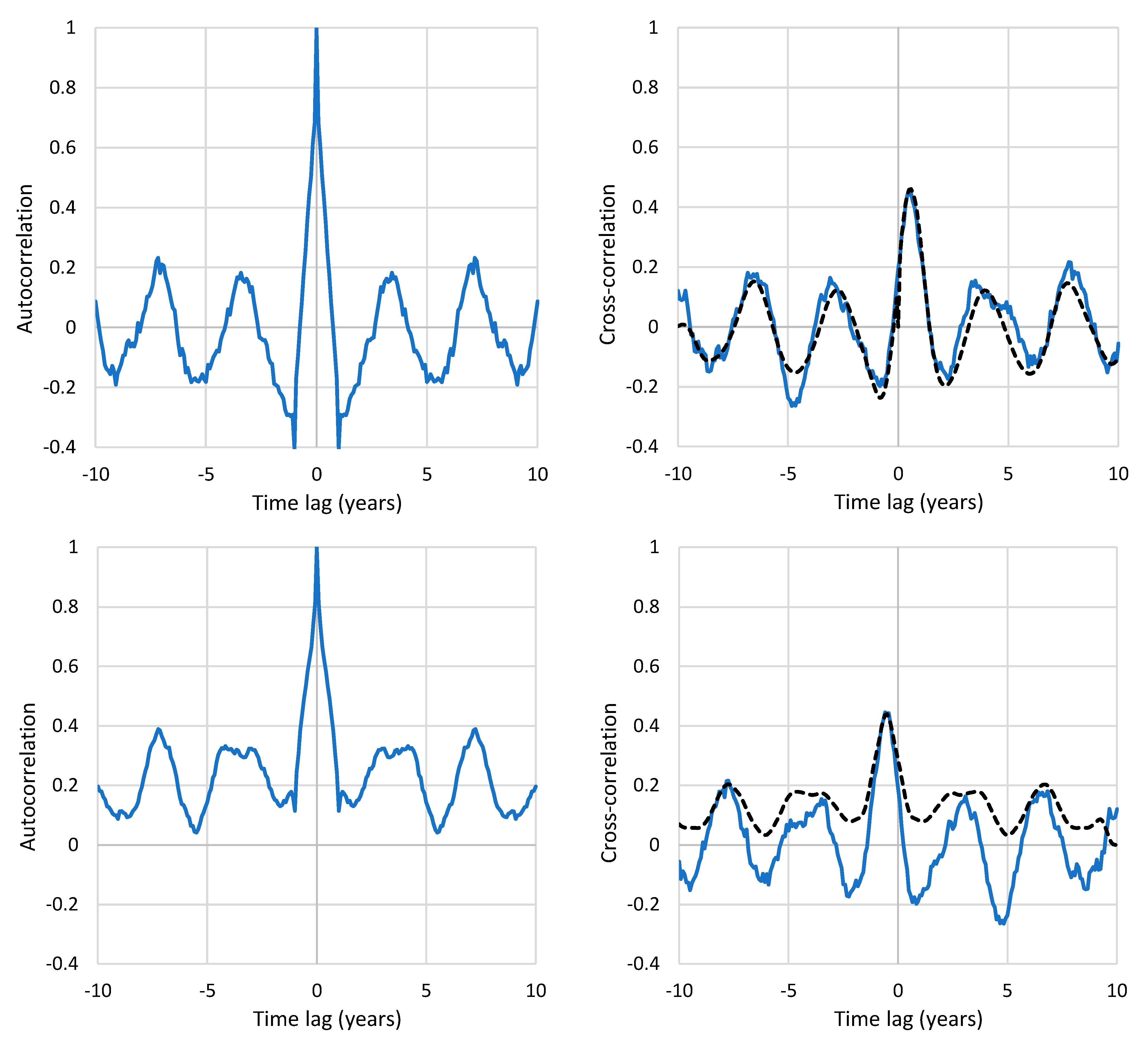
3. Data and Case Studies

To explore the T-[CO2] relationship, case studies #23 and #24 in [7] used satellite-based temperature series (UAH) for the lower troposphere and [CO2] data from Mauna Loa. Temperature data of the other two satellite levels for the troposphere were also examined, where the results were very similar to those reported for case studies #23 and #24.
Here we present additional case studies, listed in Table 1. In addition to the satellite-based temperature series in [7], here we use surface data (at 2 m) from the NCEP/NCAR Reanalysis 1 by the National Centers for Environmental Prediction (NCEP) and the National Center for Atmospheric Research (NCAR) [19], which are publicly available. The temporal coverage of the NCEP/NCAR Reanalysis 1 includes data collected four times daily to provide daily and monthly values from 1948 to the present at a horizontal resolution of 1.88° (∼210 km at the equator). It uses a state-of-the-art analysis and forecast system to perform data assimilation using observations and a numerical weather prediction model. The data assimilation and the model used are identical to the global system implemented operationally at NCEP, except for the horizontal resolution. A large subset of the data is available as daily and monthly averages.
For CO2 concentration, in addition to the Mauna Loa data set, which we updated to include the latest measurements of more than one year, we also added the South Pole data set compiled by the US National Oceanic and Atmospheric Administration (NOAA). The measurements began in 1975 and are taken for two cases, flask and in situ, of which we used the former on a mean monthly basis, except in a few cases of missing data where we filled in with in situ data.
Some of the analyses presented here refer to climate model outputs. Here we used the mean (CMIP6 mean) of the output series of the Coupled Model Intercomparison Project (CMIP6) averaged over the globe. The model outputs also go back to the past, extending over the time period of 1850–2100. When we studied past behaviors, we used the data up to 2021, as in the other case studies, but in some cases, we also used the entire data set up to 2100. In the latter case, among the scenarios provided, we used Scenario Shared Socio-Economic Pathways 245 (SSP2-4.5, [20]).
The [CO2] time series used in climate models for scenario SSP2-4.5 have also been retrieved and analyzed. We note, though, that these time series are given on an annual timescale, unlike all other data that are provided on a monthly scale.
To check whether the results of our methodology would change if we chose any particular member of the ensemble instead of the mean, we also retrieved outputs from a single model, namely the UK Earth System Model (UKESM1 [21]). For the sake of brevity of this paper, we give this latter analysis (whose results eventually do not differ from those of the CMIP6 mean) in the Supplementary Information (and therefore we do not list it in Table 1). The main case studies in which these data were used are summarized in Table 1, along with the summary indices of g j that are related to potential causality. The details of the case studies are given in the following sections. In all of them, we started by assuming a potentially hen-or-egg (HOE) causal model with a fixed number of weights g j , namely 41 (i.e., J = 20 , as in [7]).
Additional case studies examining additional data sets have also been performed but are kept out of the body of the paper and contained in Appendix A.2, Appendix A.3 and Appendix A.4. All data used are available online for free and the related links are given in the Data availability section.

4. Investigating the Maximum Time Span That Modern Data Allow

The longest time series of systematic [CO2] measurements is that of Mauna Loa, which began in 1958. The global temperature at 2 m of the NCEP/NCAR reanalysis series goes back to 1948 and thus allows studying the T-[CO2] relationship for the period 1958–2022 (two additional decades of data in comparison to those studied in [7]).
As seen in Table 1, this provided better characteristics than the UAH/Mauna Loa case examined in [7]: maximum cross correlation r y x h c = 0.56 against 0.48; explained variance e = 34% against 31%, at time lags greater than or equal to those in [7] (close to 8 months). As seen in Figure 2, again, we have a potentially causal system with the directionality being Δ T Δ l n [ C O 2 ] , while the possible causality Δ l n [ C O 2 ] Δ T can be excluded as not satisfying the necessary condition of time precedence.

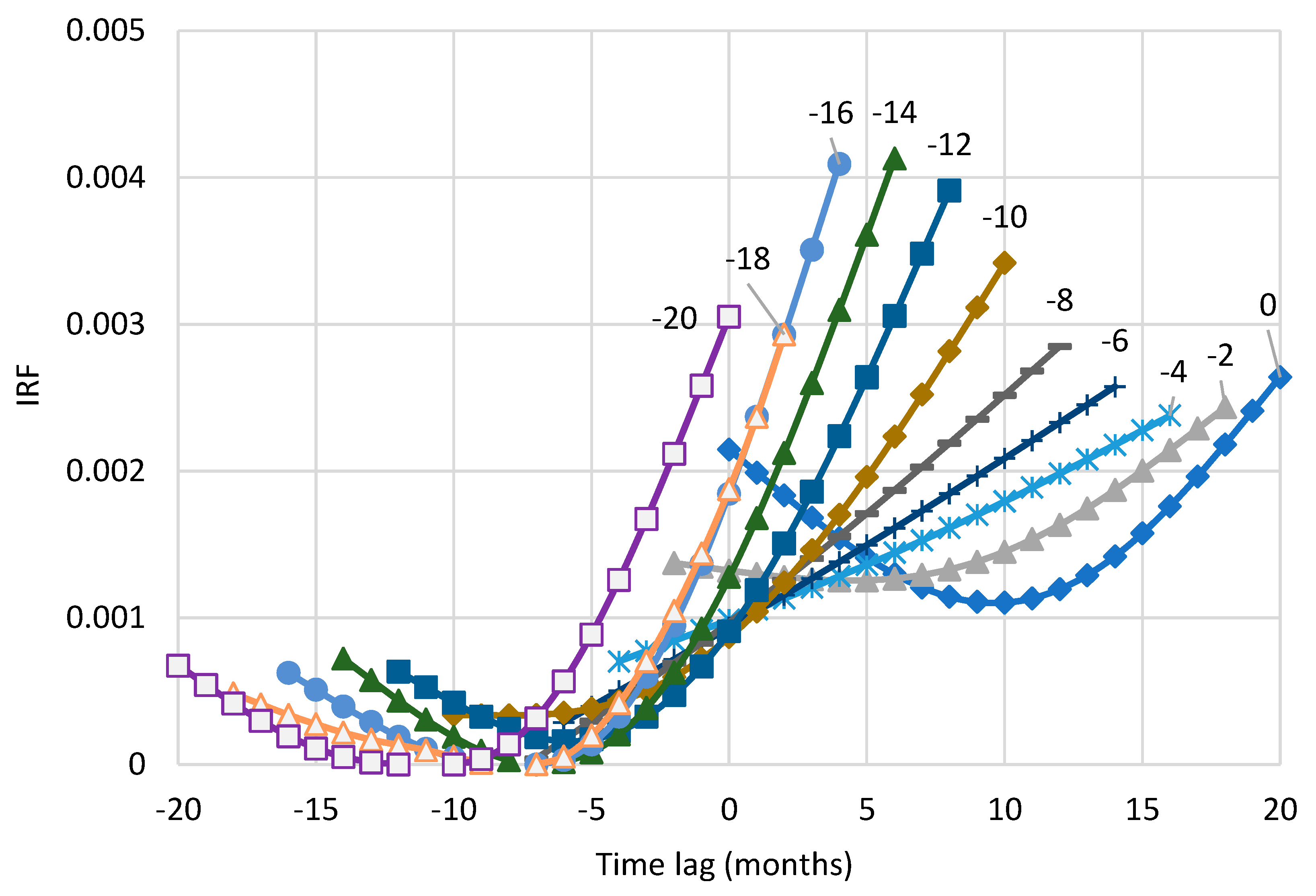
5. Investigating the Possible Effect of Seasonality

To enrich our results and also check whether seasonality, as reflected in different phases of [CO2] time series at different latitudes, could modify or possibly reverse the detected causality relationship, we have conducted an additional analysis with the South Pole [CO2] measurements, which began in 1975.
As seen in Table 1, this again provided better characteristics than the UAH/Mauna Loa case examined in [7] in terms of explained variance (e = 35% against 31%) and time lags higher than in [7] (close to 10 months). As seen in Figure 3, again, we have a potentially causal system with the directionality being Δ T Δ l n [ C O 2 ] , while again the possible causality Δ l n [ C O 2 ] Δ T can be excluded as not satisfying the necessary condition of time precedence.
Summarizing the two case studies in Section 4 and Section 5—and similarly to what we found in [7]—we note that:
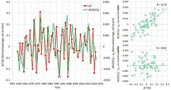
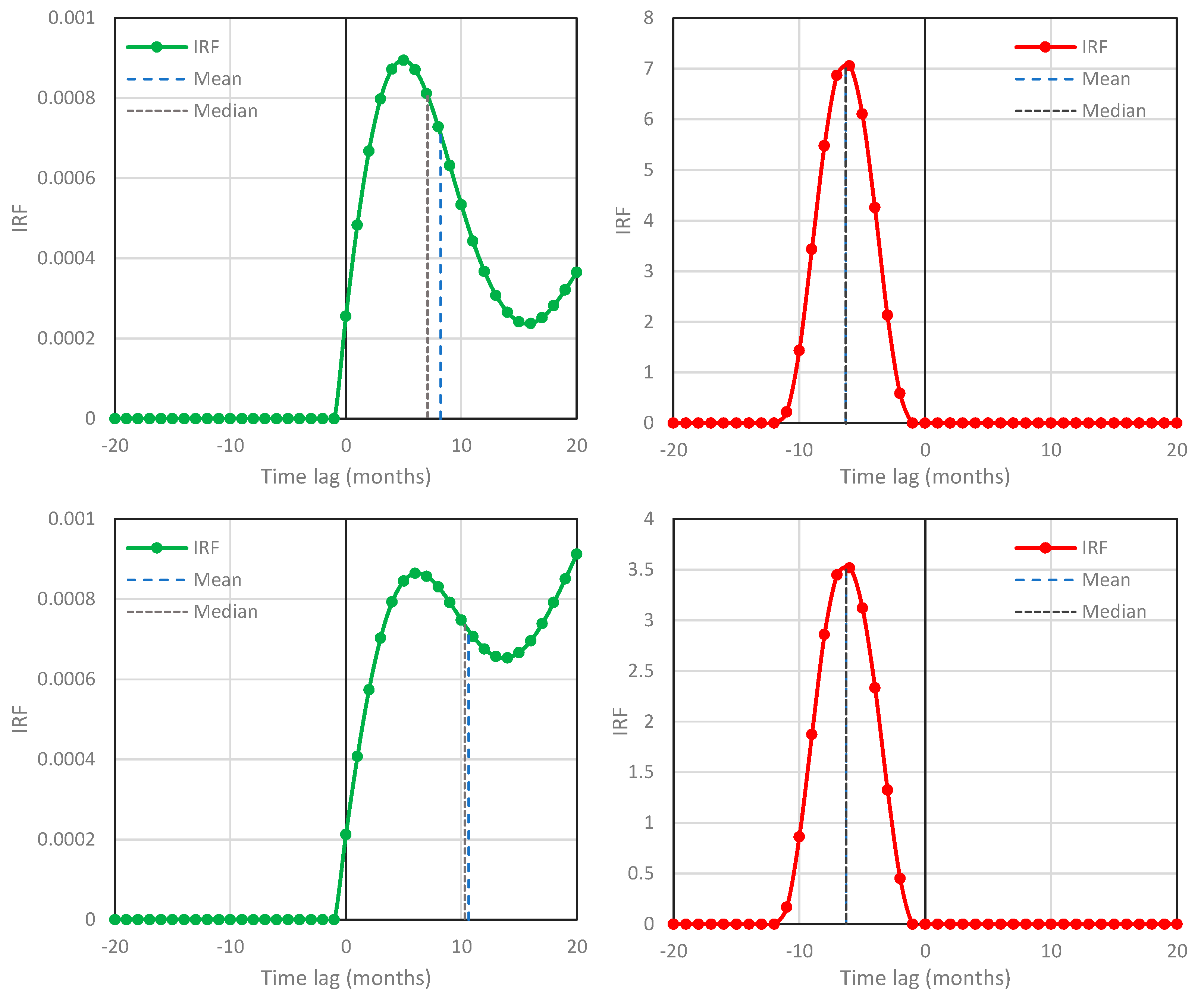
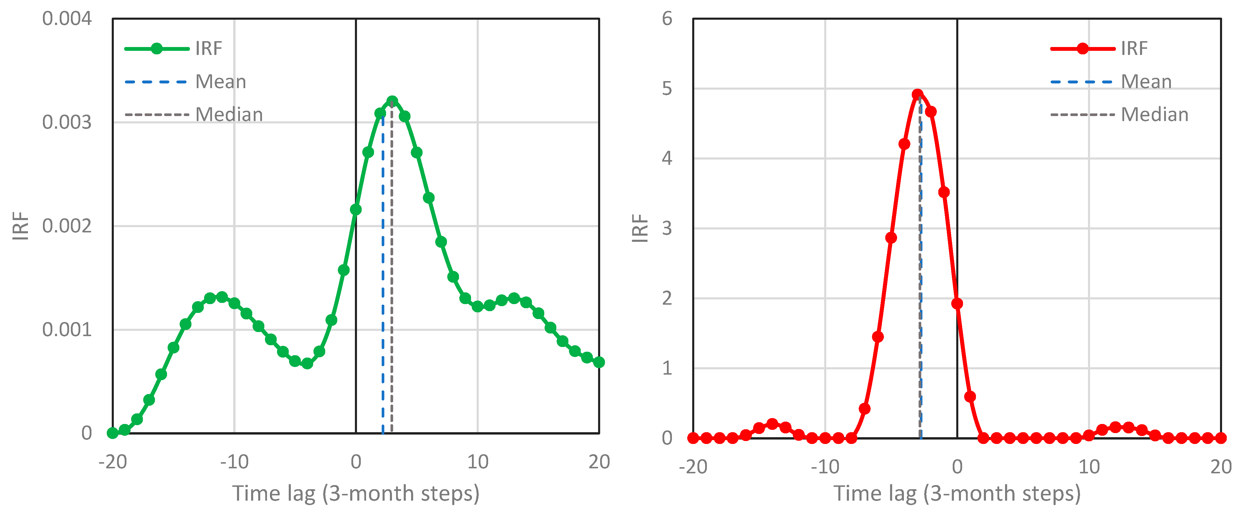
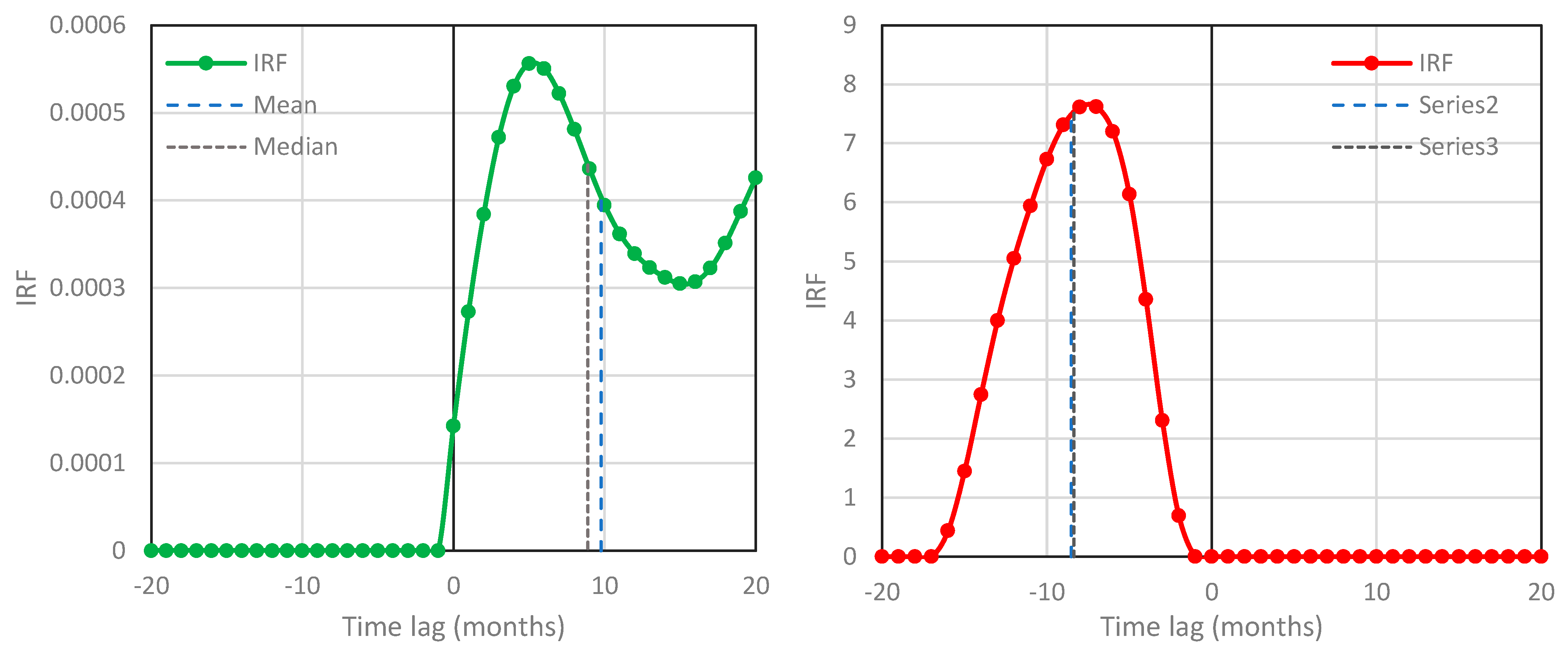
  • The system T-[CO2] appears to be potentially causal (unidirectional) in the direction Δ T Δ l n [ C O 2 ] , rather than hen-or-egg causal.
  • All characteristic time lags ( h c , μ h ,   h 1 / 2 ) are positive in the direction Δ T Δ l n [ C O 2 ] (ranging from about 7 to about 10 months), and negative in the direction Δ l n [ C O 2 ] Δ T .
  • The explained variance ratio is greater in the direction Δ T Δ l n [ C O 2 ] (about 1/3) than in the direction Δ l n [ C O 2 ] Δ T (around 1/5).

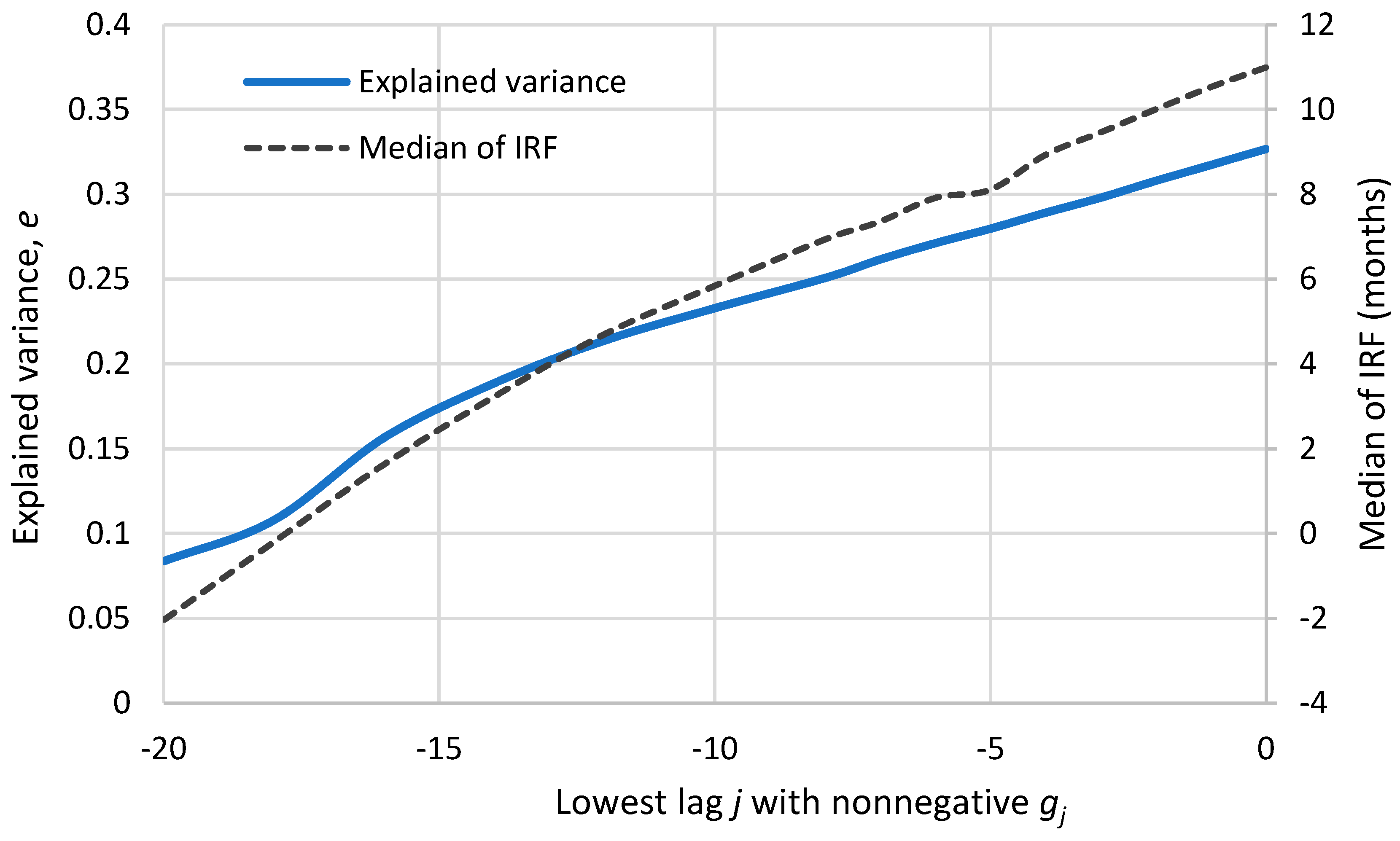
6. On the Timescale of Validity of Results

Overall, our results in this paper are those allowed by the available data at the time periods and timescales resolved by those data—more than 6 decades at the monthly scale. What would happen at other times—or if the data sets were longer and would resolve intermediate or even longer timescales—we cannot tell. The climate system is too complex to allow for hasty generalizations.
One may not exclude the case that the timescale of analysis is important in a detected potential causality relationship and that the latter would change if the timescale changed. This raises the question: up to which timescale does the validity of certain results hold? Certainly, this timescale is a fraction (not greater than 1/2) of the length of the time series. An indication can be obtained by inspecting the empirical cross-covariance function and how this compares with the theoretical one. As shown in [6], the latter ( c y x h   : = c o v y _ t + h , x _ t ) for lag h , is related to the autocovariance function of x _ , c x x h : = c o v x _ t + h , x _ t , by:
c y x ( h ) = g a c x x ( h a ) d a
Thus, c y x h can be estimated from the IRF and the empirical c x x h from the data. Figure 4 shows the autocorrelation and cross-correlation functions (which are covariances standardized by standard deviations). For the Δ T Δ l n [ C O 2 ] case (i.e., case study #3; upper panels of Figure 4), the reconstructed cross-correlation function, calculated from the IRF (seen in Figure 2) and the empirical autocorrelation function of temperature (seen in the upper left panel of Figure 4) using the discretized version of equation (7), agrees well with the empirical function for time lags up to ±10 years, i.e., spanning 20 years (1/3 of the series length). As time lag has an equivalence relationship with timescale [22], we may conclude that the potential causality relationship detected is valid for timescales of two decades. For comparison, the lower panels of Figure 4 show the reverse case, Δ l n [ C O 2 ] Δ T , (case study #4), where there is no longer good agreement between empirical and reconstructed cross-correlation, which provides additional support for the claim that the true causality link is Δ T Δ l n [ C O 2 ] .
A final observation in Figure 4 is the appearance of six peaks in 20 years, which may be interpreted as indicating a quasi-periodic behavior with an average period of 3.33 years, i.e., much different from the annual. However, this does not reflect periodicity but rather antipersistence imposed by the differencing operation, which necessarily results in some negative autocorrelations [23].
A more direct technique to deal with timescales is to average the time series on aggregate timescales and again investigate the causality relationships on these scales. This technique could detect whether a similar relationship holds for the larger timescales. In our case, since we are differencing the process, taking the average at a timescale k is equivalent to taking a difference for a time step k (notice that x 2 x 1 + x 3 x 2 + + ( x k + 1 x k ) = x k + 1 x 1 ). Therefore, to increase the timescales it suffices to increase the time step of differencing. In Figure 2, this was 1 year. Now we increase the time step of differencing, replacing the 1-year step with 2, 4, 8 and 16 years. The results are shown in Figure 5 and in Table 1 (case studies #5 to #13). They are essentially the same, except that, as the differencing time step increases, the explained variance slightly decreases (from 0.34 down to 0.27) in the direction Δ T Δ l n [ C O 2 ] , and is again much higher than that in the direction Δ l n [ C O 2 ] Δ T . The time lags increase in the former direction and are again negative in the latter direction.
A characteristic pattern is that, as the time step increases, so does the rightmost ordinate of the IRF, g 20 . This behavior, i.e., the increasing limb of g j beyond some time lag, has been explained in [7] and is an artifact of an insufficient (small) window of time lag for determining IRF. Thus, it suggests that a higher J should be used. It is quite reasonable to expect that if the differencing time step increases, so should the window size do. In particular, it is interesting to observe that in the lowest panel of Figure 5, corresponding to a differencing time step of 16 years, while the time window of IRF is only 40 months (a little more than 3 years), the IRF is a monotonously increasing function. Apparently, this is an artifact due to the too small window of time lag. In such a case, it is also reasonable to expect some nonnegative estimates of IRF ordinates for negative lags, even if the system is unidirectionally causal. Indeed, this has appeared in the case of a differencing time step of 16 years, even though the lowest panel of Figure 5 shows the purely unidirectional version of the IRF. This may create some ambiguity in the identification of causality, which we analyze and resolve in the next section.

7. Possible Ambiguities and Disambiguation

In some applications, the detection of the type of causality, unidirectional or HOE, is direct, but in other cases, it may be more difficult. This is illustrated in Figure 6. The left panel is equivalent to that of Figure 2 (left) but not neglecting some very small ordinates g j that originally the algorithm produced for negative j . The right panel is equivalent to that of Figure 5 (bottom left) but letting the optimization algorithm produce g j for negative j , which in this particular case seem not negligible. Both figure panels refer to the same processes with the differencing time step being 1 and 16 years for the left and right panels, respectively. For the 16-year step, in comparison to the IRF of Figure 5, which explains a fraction 0.31 of the variance, that of Figure 6 yields a slightly higher explained variance, 0.325, while it has some small weights at negative lags. Should we conclude then that it indicates a potential HOE, rather than unidirectional, causality? Even if our reply is affirmative, it is important to note that the characteristic lags are again positive, suggesting a principal direction Δ T Δ l n [ C O 2 ] .
However, the reply is not necessarily affirmative. The explained variance of 0.31 is associated with 21 IRF ordinates, while that of 0.325 is associated with 41 IRF ordinates. Is it reasonable to accept 20 additional parameters for an increase in the explained variance of 0.015?
Arguably, it is more reasonable in this case to change from a symmetric to a non-symmetric window of time lag. Hence, we use a window of length 21 and slide it so that the lowest nonzero time lag vary from 20 to 0. Only the case where this is 0 denotes a potential unidirectional causality, where all 20 other cases correspond to potential HOE causality. The resulting IRFs are plotted in Figure 7, while the fraction of explained variance is plotted in Figure 8 as a function of the lowest nonzero time lag. It may be noticed that the curve for the lowest time lag 0 is different from Figure 5 (bottom left). In particular, the ordinate at 0 is higher in Figure 7, thus producing a concave shape of IFR. This is a result of the fact that the window length is fixed, while the lowest ordinate no longer contributes to the roughness (no second derivative can be determined for the lowest point and thus the algorithm can increase the ordinate at 0 at no cost). In turn, the explained variance further increased to 0.327.
Clearly, the result of this investigation is a unidirectional, rather than HOE, potential causality, as the explained variance reaches its maximum when the lowest j is 0.

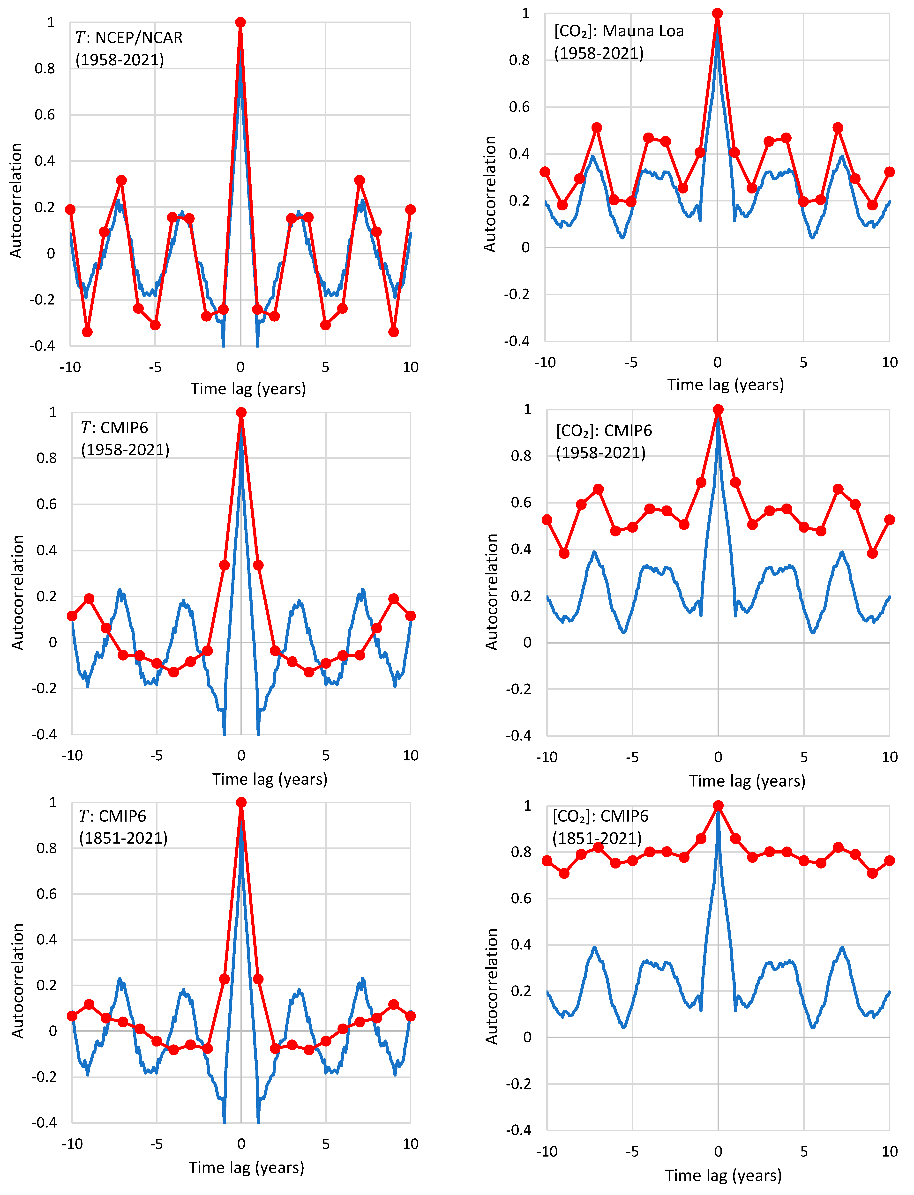
8. Comparing Observational Data with Model Results

Investigation of causality in systems that can be isolated from the environment is generally based on experiments. These are typically performed in laboratories and presuppose control actions (intervention) by the experimenter. In the absence of such intervention, it has long been regarded that we cannot say what causes what (Strotz and Wold, 1960 [24]). In complex systems, such as Earth’s climatic system, experimentation is impossible. Yet it is a widespread belief that climate models are faithful representations of the climatic system and hence offer the possibility of so-called in silico experimentation (Hannart et al. [25]). Furthermore, it has been claimed (Hannart and Naveau [26]) that “in silico experimentation [is] the only option” and that “the increasing realism of climate system models renders such an in silico approach plausible”. Such claims are epistemologically problematic. A hypothetical “causality” that is incorporated in any model, particularly of a complex system, is not necessarily identical to natural causality. In addition, the agreement of climate model outputs with reality has been questioned (e.g., [27,28,29,30,31]).
Our methodology can help with this epistemological problem in two ways. First, it provides a different option to test causality, showing that the so-called in silico experimentation is not the only option as claimed. Second, it can additionally test whether there is indeed realism in the representation of causality of the climatic system by the climate models. As already stated in the Introduction, our methodology, regardless of the detection of causality per se, can define a type of data analysis that could shed light on modeling performance by comparing observational data with model results. This is particularly useful in the case of climate modeling. In other words, it could help in verifying or falsifying the commonly accepted theory, which is incorporated in the climate models.
Specifically, we can test whether the climate model results are consistent with the findings of our T-[CO2] causality analysis, which is based on measurements. To this aim, we use climate model outputs as specified in Section 3, in the case studies #16 to #23 detailed in Table 1. Numerical results of our analysis are shown in Table 1, and graphical depictions of IRFs are shown in Figure 9 for the cases in which no roughness constraint is used and in Figure 10 for the cases in which the roughness constraint is used.
Unfortunately, and unlike the [CO2] time series of measurements, which are available on a monthly scale, the SSP2 [CO2] data series is provided on an annual scale. Therefore, case studies #16 to #23 had to be made on an annual scale. If we did the analysis for the period 1958–2021, as in case studies #3 and #4 (NCEP/NCAR Reanalysis temperature at 2 m; and Mauna Loa [CO2] time series), the annual data would be too few to support estimation of the IRFs (63 data values to estimate 41 coefficients). Therefore, in case studies #16 to #23 we extended the period back to 1850, which is covered by the climate model outputs. We performed separate analyses for the periods 1850–2100 (entire period covered by climate models) and 1850–2021 (only the past).
The results of these case studies allow us to make the following observations.
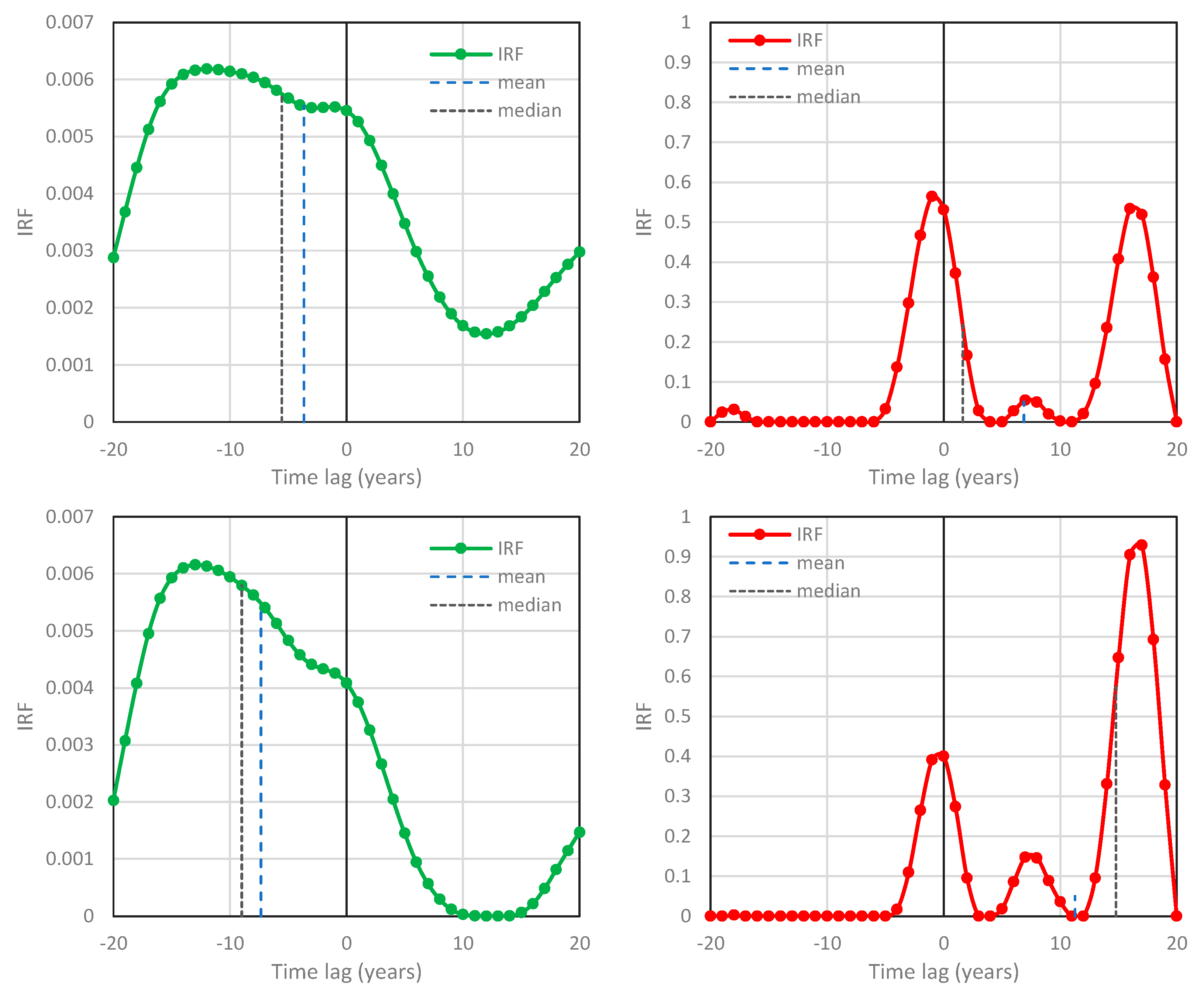
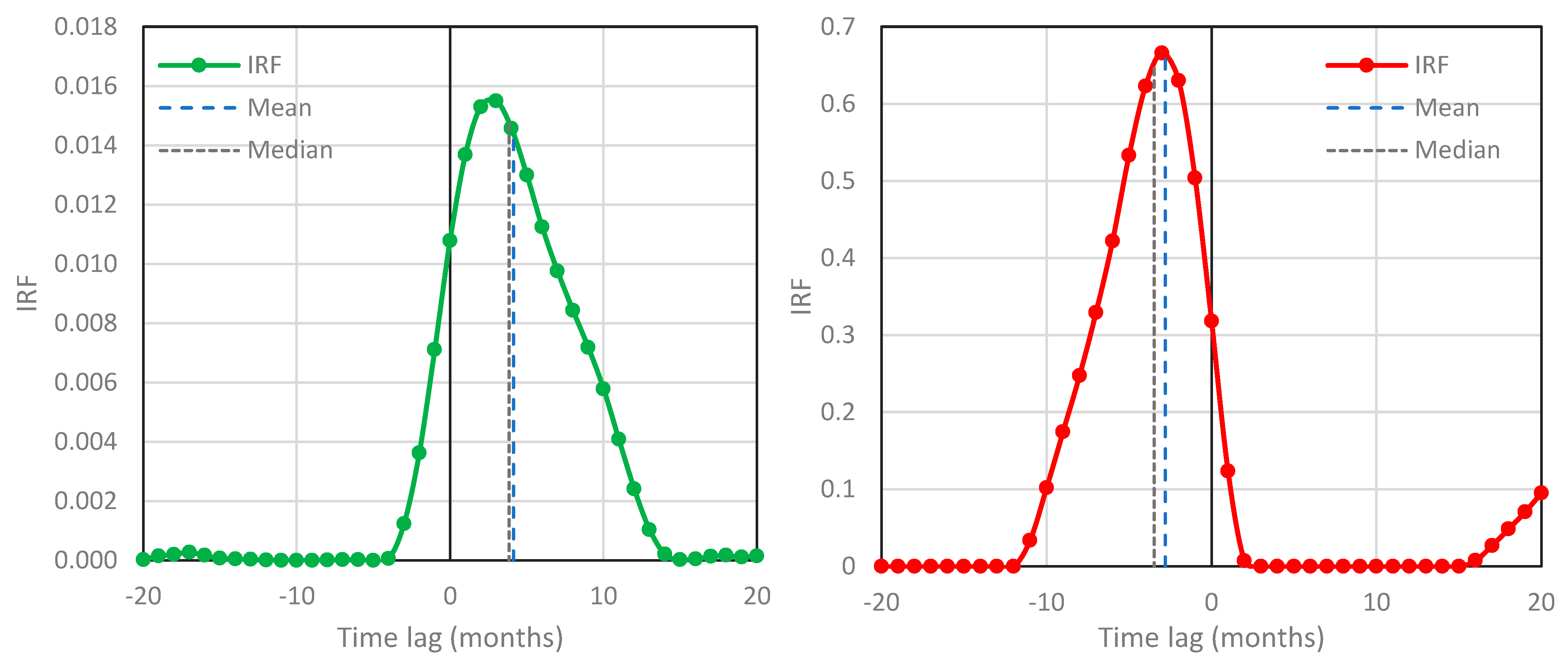
  • There is no essential difference between the results for the periods 1850–2100 and 1850–2021.
  • While, as expected, the IRFs differ if they are calculated with or without constraining roughness, the characteristic lags are similar in the two cases (with the exception of h 1 / 2 in cases #17 and #21).
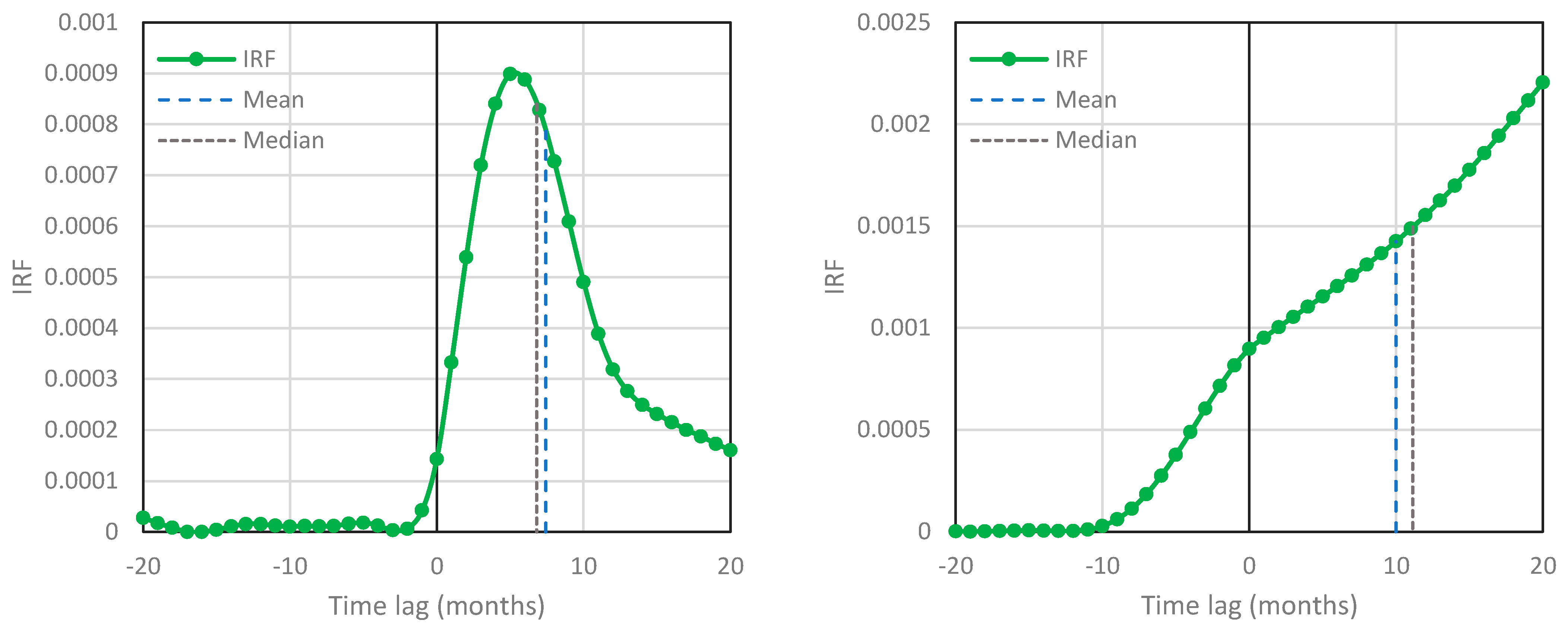
  • In all cases, the lags are negative in the direction Δ T Δ l n [ C O 2 ] and positive in the direction Δ l n [ C O 2 ] Δ T , suggesting a HOE causality with principal direction Δ l n C O 2   Δ T .
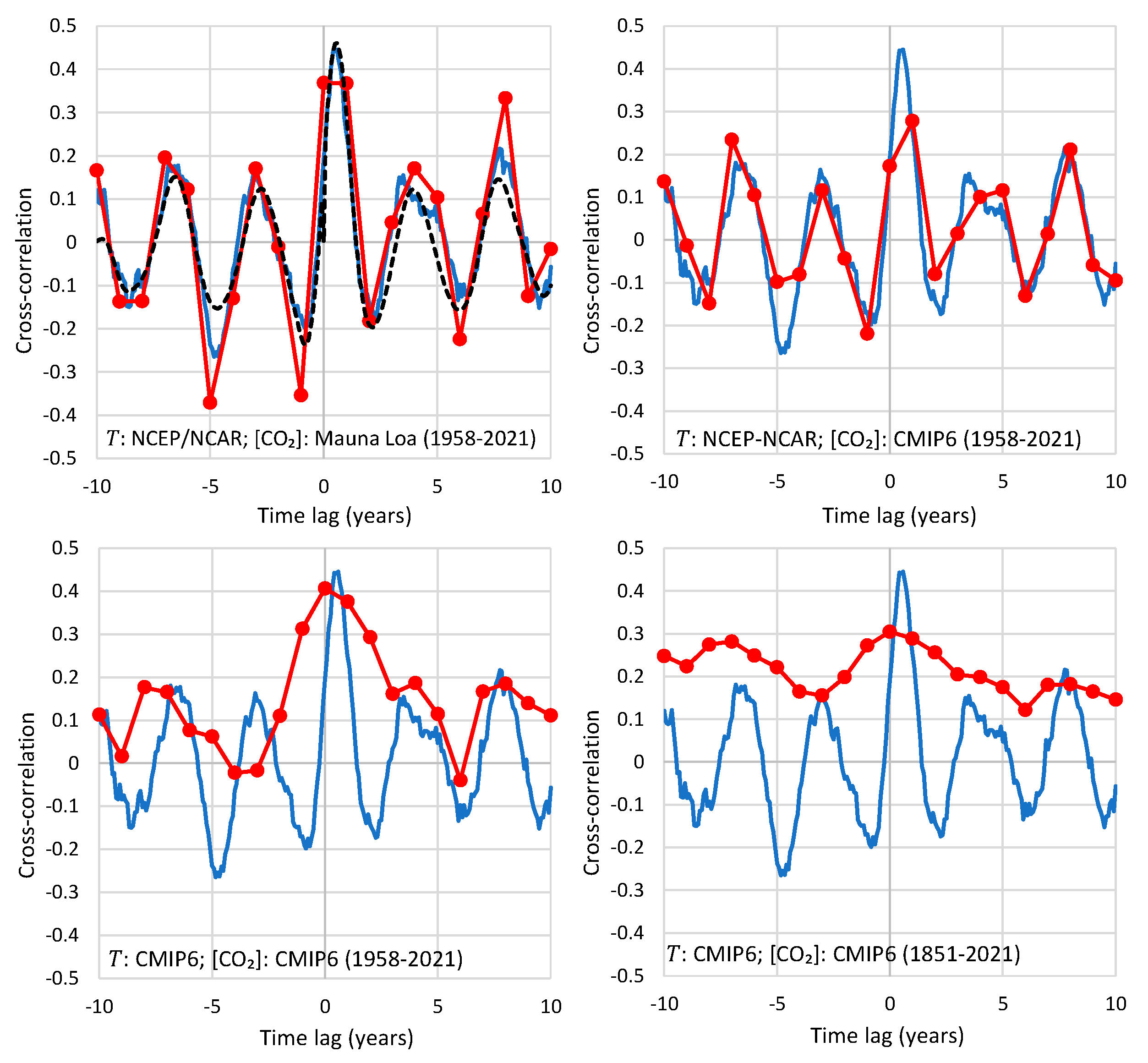
  • Clearly, the finding in point 3, resulting from climate model outputs, is opposite to the results found when real measurements are used (NCEP/NCAR Reanalysis temperature and Mauna Loa [CO2] time series).
  • Oddly, while the principal direction suggested by the models is Δ l n [ C O 2 ] Δ T , the explained variance is impressively low (10–15%) in this direction and impressively high (reaching 90%) in the opposite direction, Δ T Δ l n [ C O 2 ] .
One may argue that the main result of this analysis, i.e., the point 4 above, may be affected by the difference in the study periods, i.e., 1958–2021 for the real measurements and 1850–2021 for the model outputs. To examine whether the origin of the different behavior is the time period or the system dynamics (actual vs. modeled), we performed an additional analysis, graphically depicted in Figure 11 and Figure 12.
The upper left panel of Figure 11 is similar to that in Figure 4 (upper right), where, in addition, we have plotted the empirical cross-correlation function for the same data but averaged at the annual scale. This agrees relatively well with the empirical function at the monthly scale, which provides a basis for the comparisons that follow.
The empirical cross-correlation function at the monthly scale is copied in all other panels of Figure 11 and serves as a basis for the comparisons. In the upper right panel, where we replaced the Mauna Loa time series for [CO2] with the CMIP6 time series for the same period, 1958–2021, while keeping the NCEP/NCAR time series for T, there is still agreement of the annual with the monthly cross-correlations. However, when we also replace the NCEP/NCAR time series for T with the CMIP6 series (lower left plot), the two plots decouple. The decoupling is even more prominent if we go to the longer period 1850–2021 (lower right panel).
Similar observations can be made about autocorrelations in Figure 12. In particular, the CMIP6 autocorrelation of T decouples from the actual one for both periods 1958–2021 and 1850–2021, while the two latter do not differ substantially from each other. These observations allow us to assert that the main cause of disagreement has to do with problems with the modeling of system dynamics rather than the time period of study.

9. Discussion and Further Results

The mainstream assumption of the causality direction [CO2] → T makes a compelling narrative, as everything is blamed on a single cause, the human CO2 emissions. Indeed, this has been the popular narrative for decades. However, popularity does not necessarily mean correctness, and here we have provided strong arguments against this assumption. Since we have identified atmospheric temperature as the cause and atmospheric CO2 concentration as the effect, one may be tempted to ask the question: What is the cause of the modern increase in temperature? Apparently, this question is much more difficult to reply to, as we can no longer attribute everything to any single agent.
We do not claim to have the answer to this question, whose study is far beyond the article’s scope. Neither do we believe that mainstream climatic theory, which is focused upon human CO2 emissions as the main cause and regards everything else as feedback of the single main cause, can explain what happened on Earth for 4.5 billion years of changing climate.
Nonetheless, as a side product, in the Appendices to the paper, we provide several indications of the following:
  • The dependence of the carbon cycle on temperature is quite strong and indeed major increases of [CO2] can emerge as a result of temperature rise. In other words, we show that the natural [CO2] changes due to temperature rise are far larger (by a factor > 3) than human emissions (Appendix A.1).
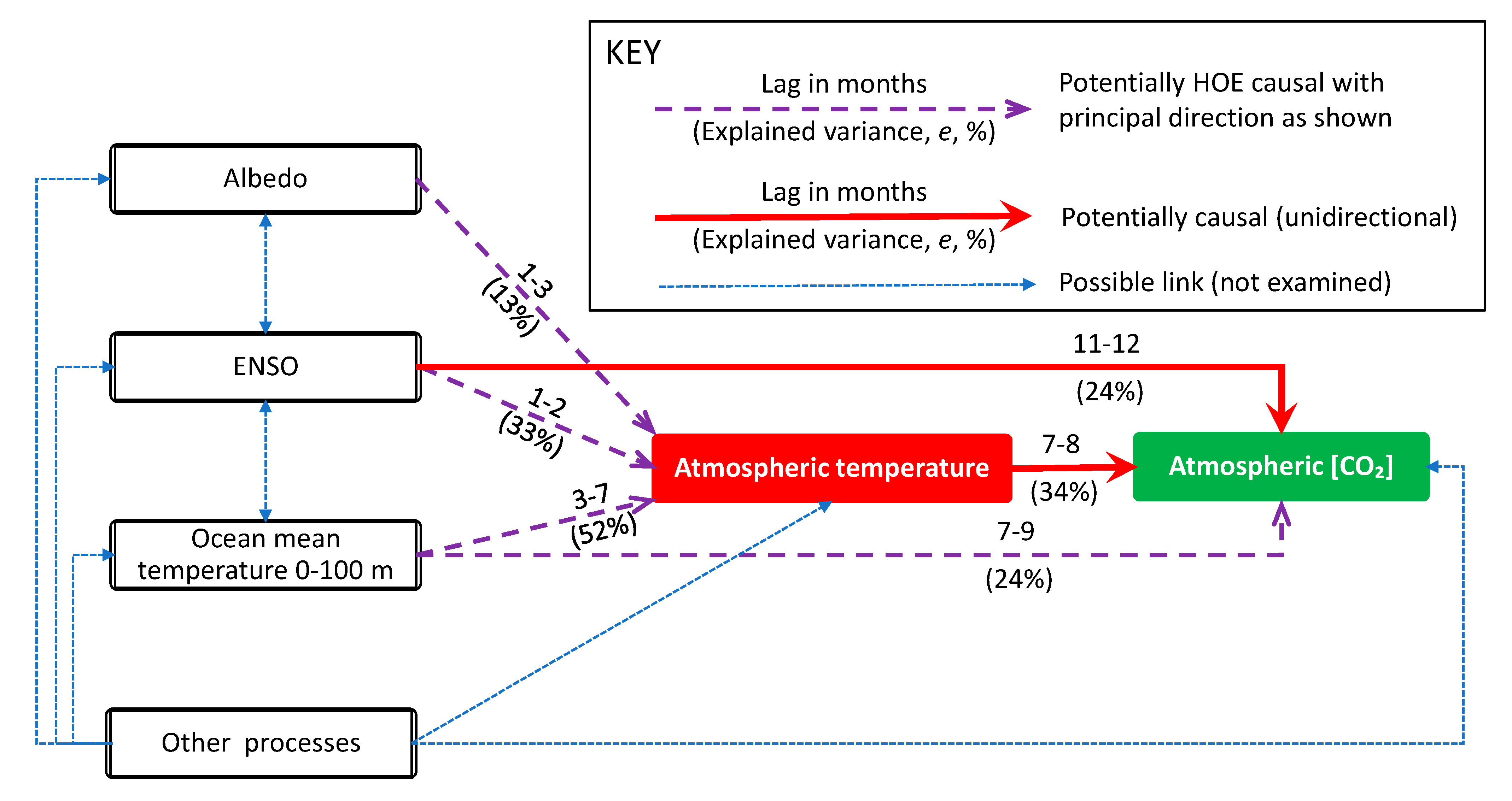
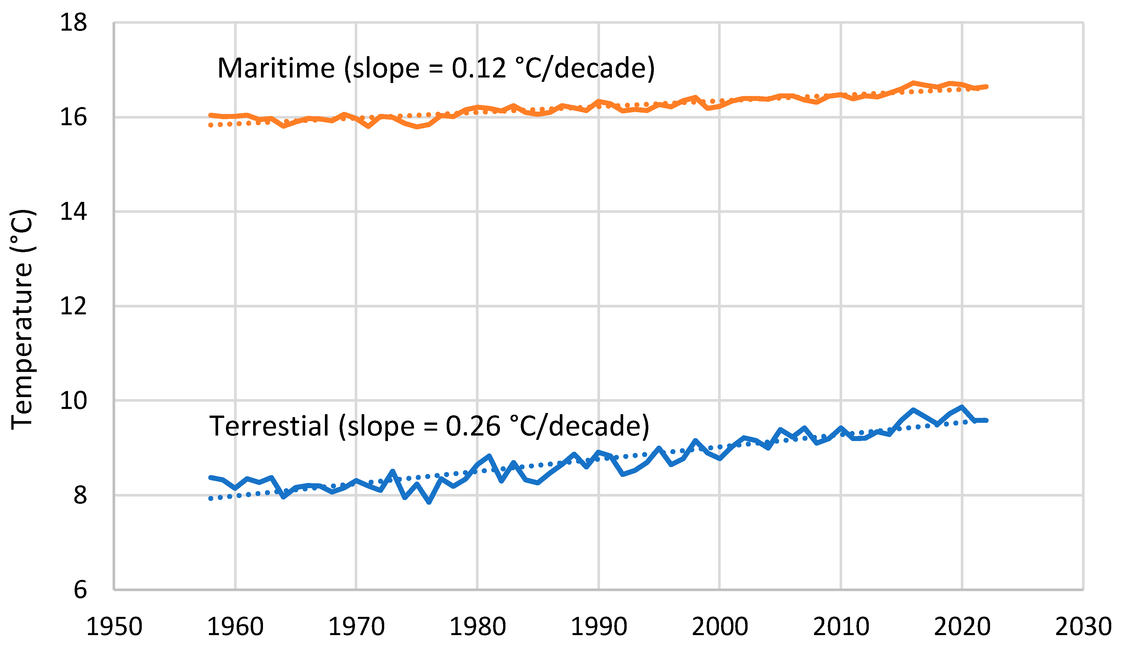
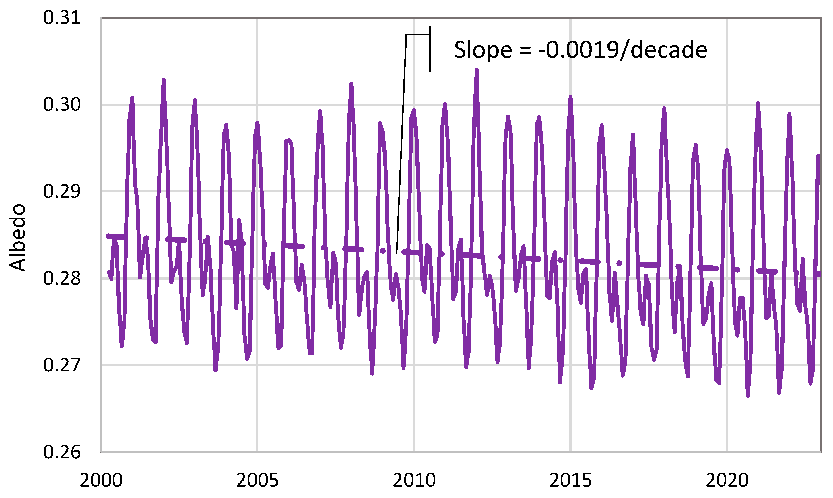
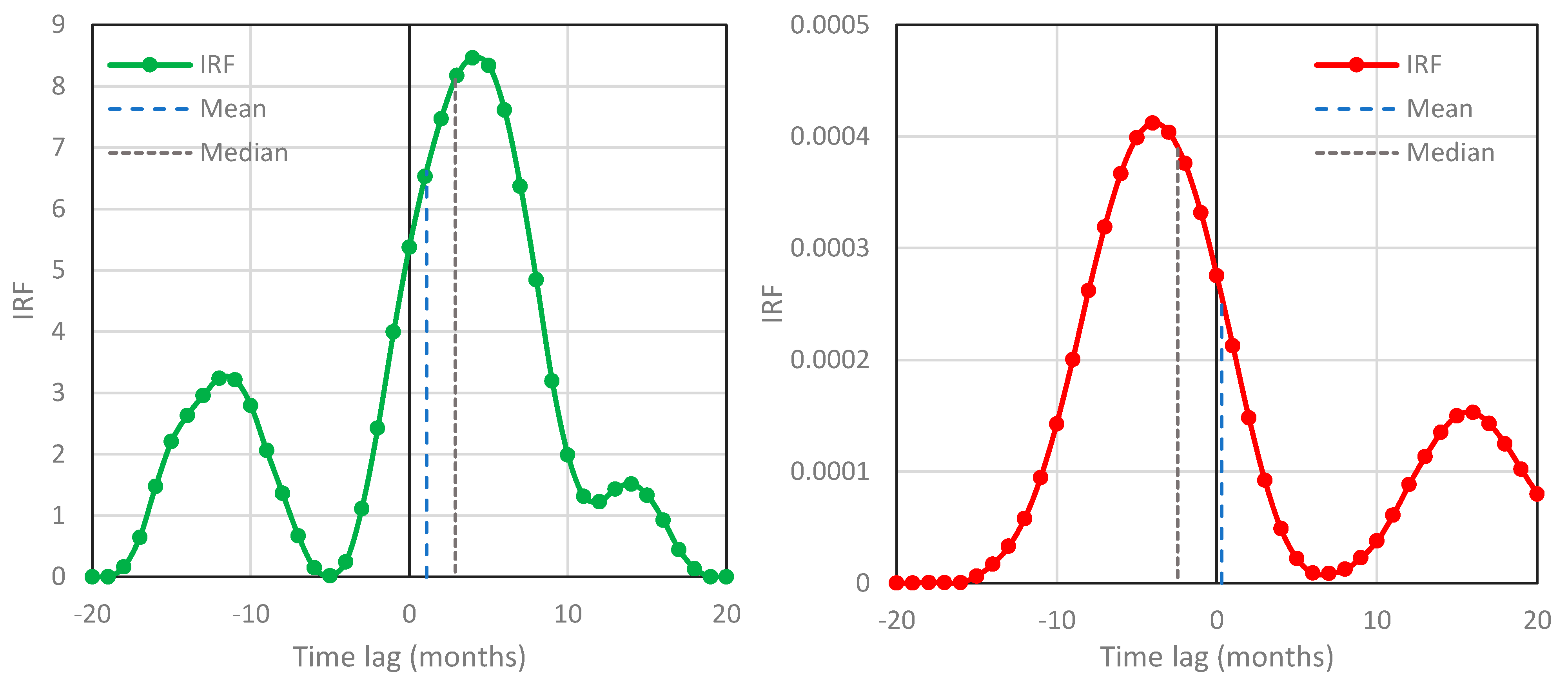
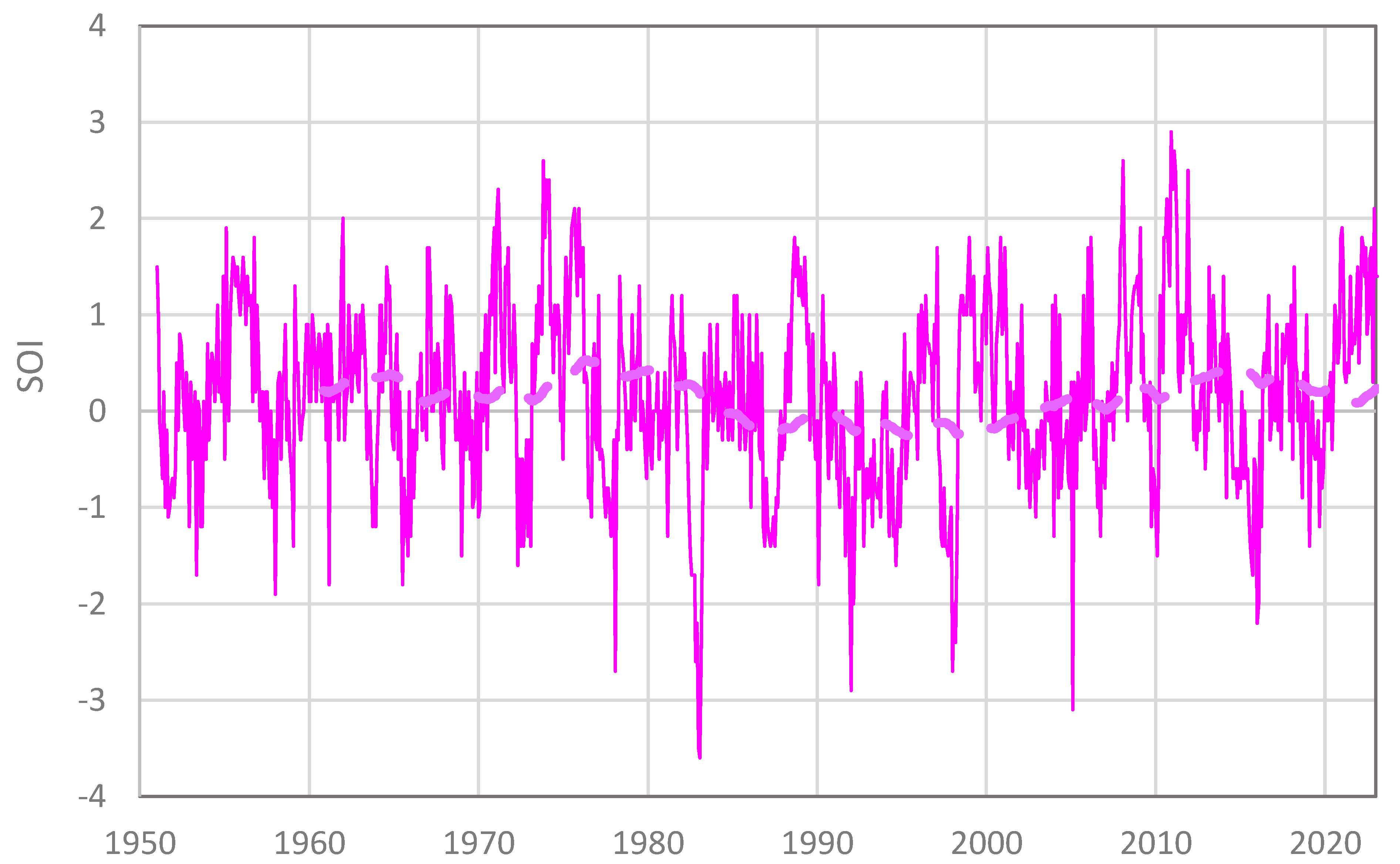
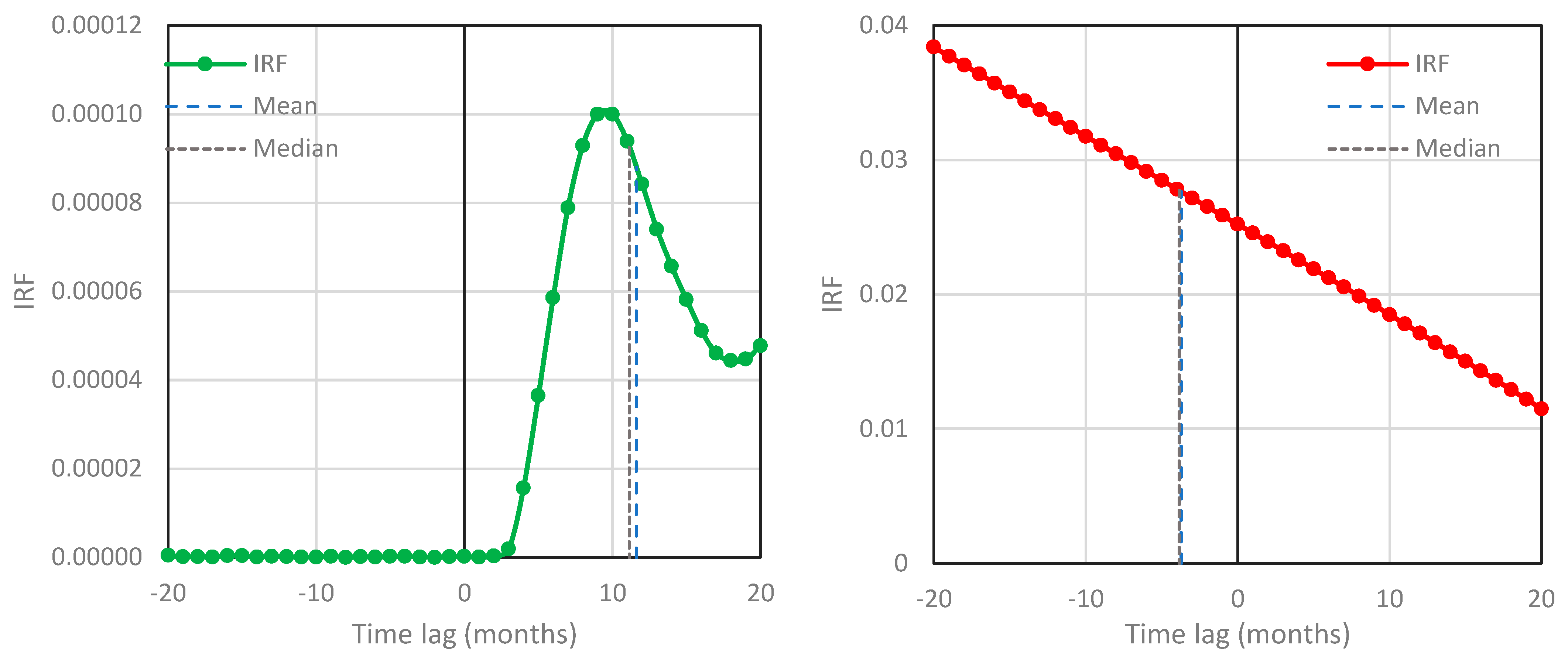
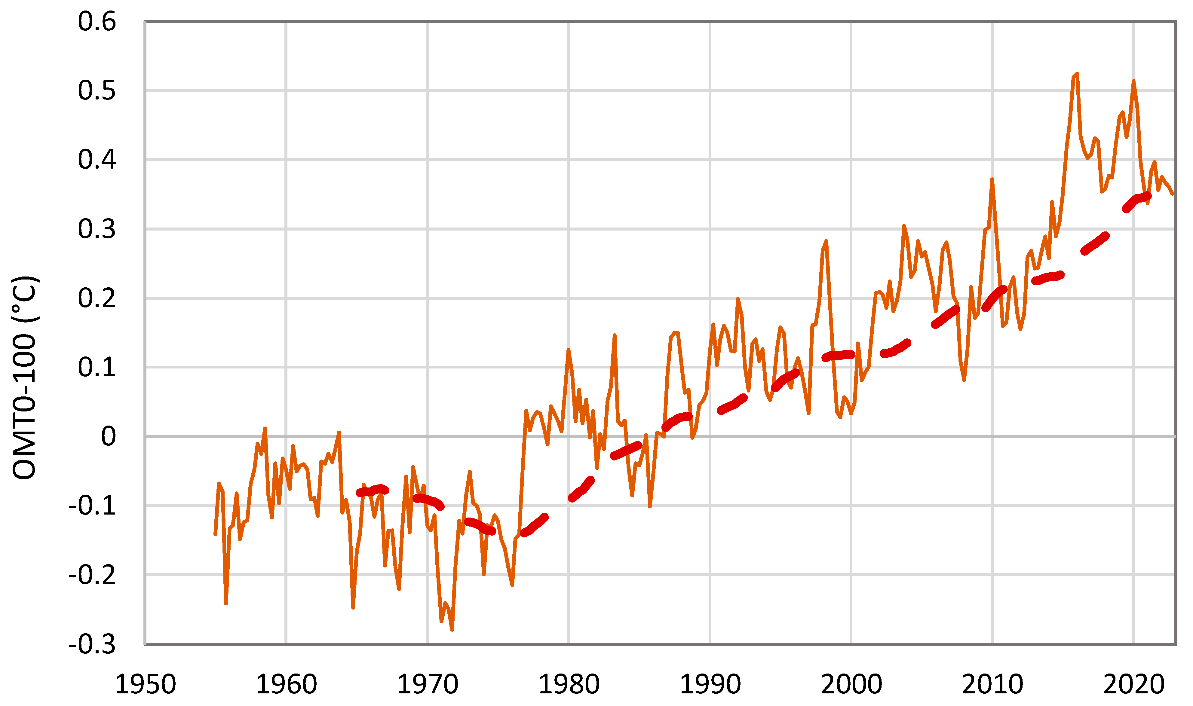
  • There are processes, such as the Earth’s albedo (which is changing in time as any other characteristic of the climate system), the El Niño–Southern Oscillation (ENSO) and the ocean heat content in the upper layer (represented by the vertically averaged temperature in the layer 0–100 m), which are potential causes of the temperature increase, unlike what is observed with [CO2], their changes precede those of temperature (Appendix A.2, Appendix A.3 and Appendix A.4).
  • On a large timescale, the analysis of paleoclimatic data supports the primacy of the causal direction T → [CO2], even though some controversy remains about this issue (Appendix A.5).
In terms of the carbon cycle (point 1 above), several physical, chemical, biochemical and human processes are involved in it. The human CO2 emissions due to the burning of fossil fuels have largely increased since the beginning of the industrial age. However, the global temperature increase began succeeding the Little Ice Period, at a time when human CO2 emissions were very low. To cast light on the problem, we examine the issue of CO2 emissions vs. atmospheric temperature further in the Supplementary Information, where we provide evidence that they are not correlated with each other. The outgassing from the sea is also highlighted sometimes in the literature among the climate-related mechanisms. On the other hand, the role of the biosphere and biochemical reactions is often downplayed, along with the existence of complex interactions and feedback. This role can be summarized in the following points, examined in detail and quantified in Appendix A.1.
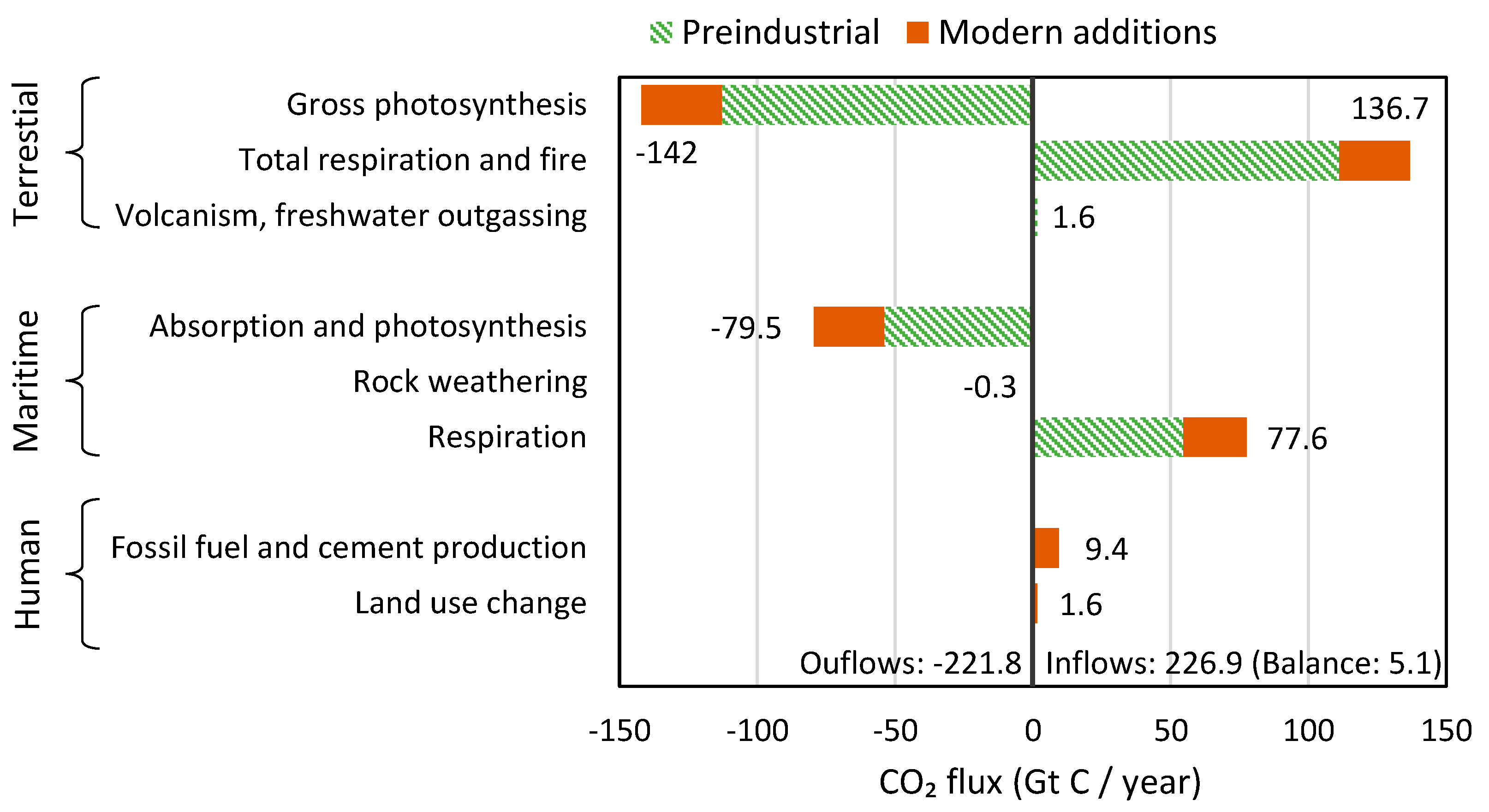
  • Terrestrial and maritime respiration and decay are responsible for the vast majority of CO2 emissions [32], Figure 5.12.
  • Overall, natural processes of the biosphere contribute 96% to the global carbon cycle, the rest, 4%, being human emissions (which were even lower in the past [33]).
  • The biosphere is more productive at higher temperatures, as the rates of biochemical reactions increase with temperature, which leads to increasing natural CO2 emission [2].
  • Additionally, a higher atmospheric CO2 concentration makes the biosphere more productive via the so-called carbon fertilization effect, thus resulting in greening of the Earth [34,35], i.e., amplification of the carbon cycle, to which humans also contribute through crops and land-use management [36].
In addition to the biosphere, there are other factors that drive the Earth’s climate in periodic and non-periodic way. Orbital parameters of Earth’s revolution change quasi-cyclically in a multi-millennial scale (variations in eccentricity, axial tilt, and precession of Earth’s orbit), as interpreted by Milanković [37,38,39,40,41], and changes in the orbit geometry influence the amount of insolation. The non-periodic drivers of the Earth’s climate variability include volcanic eruptions and collisions with large extraterrestrial objects, e.g., asteroids. An important climate driver is water in its three phases [33]. Another apparent factor is solar activity (including solar cycles) and the solar radiation (im)balance on Earth (e.g., albedo changes; see [33] and Appendix A.2). Notably, a recent study [42], by assessing 20 years of direct observations of energy imbalance from Earth-orbiting satellites, showed that the global changes observed appear largely from reductions in the amount of sunlight scattered by Earth’s atmosphere.
ENSO and ocean heating, both of which affect temperature, are examined in Appendix A.3 and Appendix A.4, respectively. The results of Appendix A.2, Appendix A.3 and Appendix A.4 are summarized in the schematic of Figure 13. Changes in all three examined processes, albedo, ENSO and the upper ocean heat, precede in time the changes in temperature and even more so those in [CO2]. Generally, the time lags shown in Figure 13 complete a consistent picture of potential causality links among climate processes and always confirm the T [ C O 2 ] direction.
The examined processes in the Appendices are internal to the climatic system. Other processes affecting T, not examined here, could also be external (e.g., solar and astronomical [43,44] and geological [45,46,47,48,49]). Generally, in complex systems, an identified causal link, even though it gives some explanation of a phenomenon, raises additional questions, e.g., what caused the change in the identified cause, etc. In turn, causal links in complex systems may form endless sequences. For this reason, it is naïve to expect complete answers to problems related to complex systems or to assume that a complex system is in permanent equilibrium and that an external agent is needed to “kick” it out of the equilibrium and produce change. Yet the investigation of a single causal link between two processes, as is the focus of this paper, provides useful information, with possible significant scientific, technical, practical, epistemological and philosophical implications. These are not covered in this paper. Readers interested in epistemological and philosophical aspects of causality are referred to Koutsoyiannis et al. [6], while those interested in the perennial changes in complex systems are referred to Koutsoyiannis [50,51].
As already clarified, the scope of our work is not to provide detailed modeling of the processes studied but to check causality conditions. We highlight the fact that the relationship we established explains only about 1/3 of the actual variance of Δ l n [ C O 2 ] . This is not negligible for investigating causality, but also leaves a margin for many other climatic factors to act.
Nonetheless, our results can certainly be improved if we change our scope to more detailed modeling. To illustrate this, we provide the following toy model. Based on our result that the T-[CO2] system is potentially causal with direction Δ T Δ l n [ C O 2 ] , we estimate Δ l n [ C O 2 ] as
Δ l n [ C O 2 ] = j = 0 20 g j Δ T τ j + μ v
and we proceed a step further, assuming that the mean μ v also depends on past temperature, averaged at timescale m, i.e.,
μ v = α T m T 0
where T m is the average temperature of the previous m years, and α and T 0 are constants (parameters). Such a simple linear relationship is supported by the above-listed points related to the productivity of the biosphere. Equation (9) will result in negative values μ v if T m < T 0 and positive otherwise.
By re-evaluating the IRF coordinates g j simultaneously with the parameters of Equation (9), we find the modified version of the IRF plotted in Figure 14. The optimized additional parameters are m = 4 (years), α = 0.0034 ,   T 0 = 285.84   K . Similarly to [6], we used a common spreadsheet software solver to perform the optimization, adding the two parameters α and T 0 to the unknown coordinates g j of the IRF and performing the (nonlinear) optimization for all unknowns ( m was found by trial-and-error). A graphical comparison of the actual Δ l n [ C O 2 ] and [ C O 2 ] with those simulated by the model of Equations (8) and (9) is given in Figure 15. The explained variance for Δ l n [ C O 2 ] was drastically increased from 34% to 55.5% and that for [ C O 2 ] is an impressive 99.9%.
For the convenience of the readers who are interested in repeating the calculations, we also give a parametric expression of IRF and summarize the toy model as:
Δ l n [ C O 2 ] = j = 0 20 g j Δ T τ j + μ v , g j = 0.00076   j 0.67 e 0.2 j / K , μ v = 0.0034   T 4 / K 285.84
(where K is the unit of kelvin).
We emphasize, however, that we do not exploit the impressive result of explained variance of 99.9% to assert that we have built a decent model, even though this toy model is both accurate (in the lower panel of Figure 15, the simulated curve is indistinguishable from the actual) and parsimonious (the model expression in (10) contains only 5 fitted parameters). We prefer to highlight the fact that the hugely complex climate system entails high uncertainty, and its study needs reliable data that provide the basis for the modeling and testing of hypotheses.

10. Conclusions

With reference to points 1–7 of the Introduction setting the paper’s scope, the results of our analyses can be summarized as follows.
  • All evidence resulting from the analyses of the longest available modern time series of atmospheric concentration of [CO2] at Mauna Loa, Hawaii, along with that of globally averaged T, suggests a unidirectional, potentially causal link with T as the cause and [CO2] as the effect. This direction of causality holds for the entire period covered by the observations (more than 60 years).
  • Seasonality, as reflected in different phases of [CO2] time series at different latitudes, does not play any role in potential causality, as confirmed by replacing the Mauna Loa [CO2] time series with that in South Pole.
  • The unidirectional T l n [ C O 2 ] potential causal link applies to all timescales resolved by the available data, from monthly to about two decades.
  • The proposed methodology is simple, flexible and effective in disambiguating cases where the type of causality, HOE or unidirectional, is not quite clear.
  • Furthermore, the methodology defines a type of data analysis that, regardless of the detection of causality per se, assesses modeling performance by comparing observational data with model results. In particular, the analysis of climate model outputs reveals a misrepresentation of the causal link by these models, which suggest a causality direction opposite to the one found when the real measurements are used.
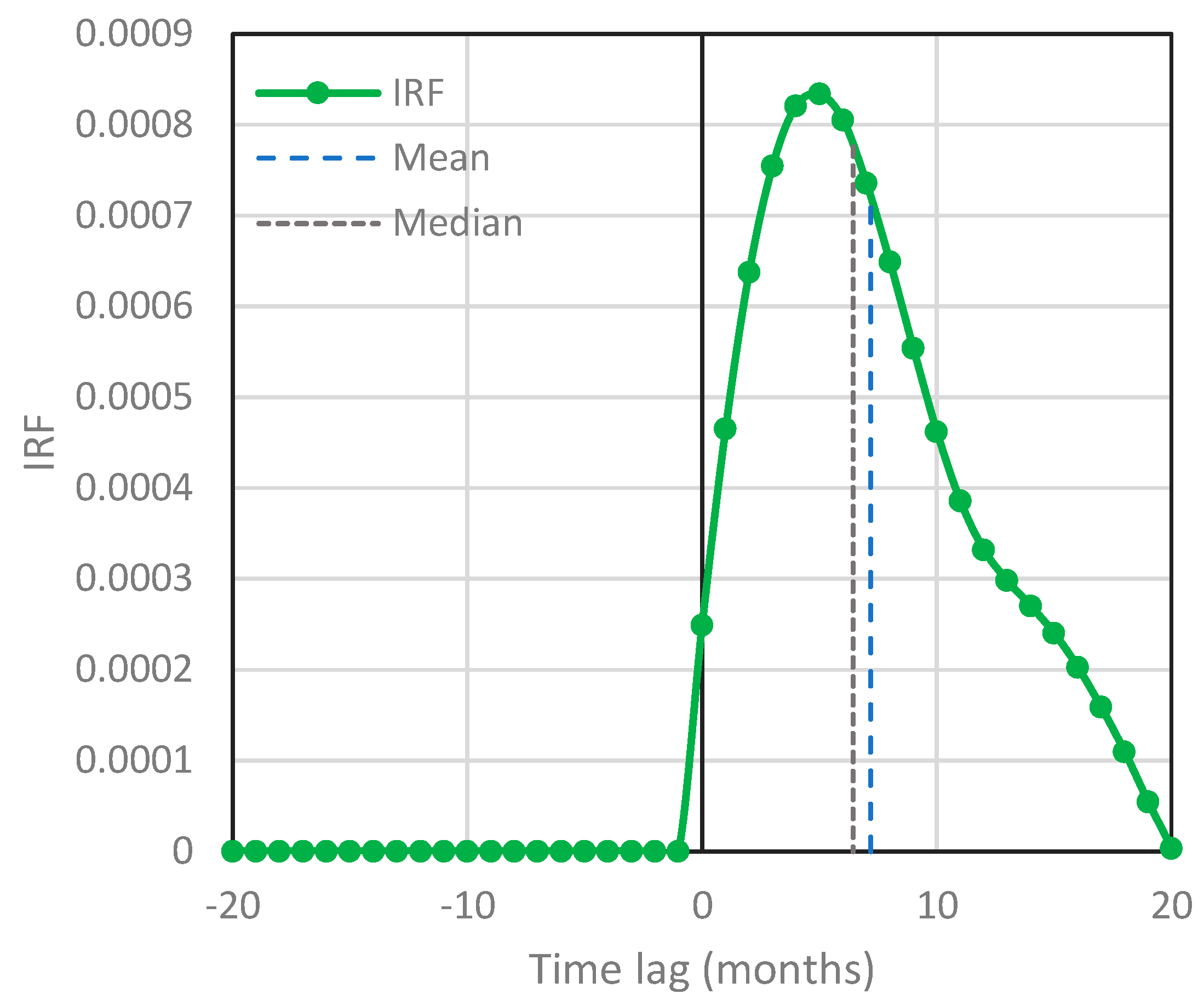
  • Extensions of the scope of the methodology, i.e., from detecting possible causality to building a more detailed model of stochastic type, are possible, as illustrated by a toy model for the T-[CO2] system, with explained variance of [CO2] reaching an impressive 99.9%.
  • While some of the findings of this study seem counterintuitive or contrary to mainstream opinions, they are logically and computationally supported by arguments and calculations given in the Appendices.
Overall, the stochastic notion of a causal system, based on the concept of the impulse response function, proved to be very effective in studying demanding causality problems. A crucial characteristic of our methodology is its direct use of the data per se, in contrast with other methodologies that are based on uncertain estimates of autocorrelation functions or on the more uncertain tool of the power spectrum, i.e., the Fourier transform of the autocorrelation function. The methodology has the potential for further advances, as we first reported here (e.g., the asymmetric time lag window, the definition of a type of data analysis to be used in assessing modeling performance, and the extensions of its scope from detecting possible causality to building a more detailed model).

Supplementary Materials

The following supporting information can be downloaded at: https://www.mdpi.com/article/10.3390/sci5030035/s1: Section SI1, Additional analysis of climate model behavior; Section SI2, On correlations of temperature with CO2 emissions.

Author Contributions

Conceptualization, D.K.; methodology, D.K., C.O., Z.W.K. and A.C.; software, D.K.; validation, D.K., C.O., Z.W.K. and A.C.; formal analysis, D.K., C.O., Z.W.K. and A.C.; investigation, D.K., C.O., Z.W.K. and A.C.; data curation, D.K.; writing—original draft preparation, D.K., C.O., Z.W.K. and A.C; writing—review and editing, D.K., C.O., Z.W.K. and A.C.; visualization, D.K.; supervision, D.K., C.O., Z.W.K. and A.C.; project administration, D.K. All authors have read and agreed to the published version of the manuscript.

Funding

This research received no external funding but was motivated by the scientific curiosity of the authors.

Institutional Review Board Statement

Not applicable.

Informed Consent Statement

Not applicable.

Data Availability Statement

All data used in the paper are available online for free. The NCEP/NCAR temperature time series and the Mauna Loa CO2 time series are readily available on a monthly scale from the climexp (http://climexp.knmi.nl/ (accessed on 1 January 2023) platform, namely from http://climexp.knmi.nl/data/inair_0-360E_-90-90N_n.dat and http://climexp.knmi.nl/getindices.cgi?WMO=CDIACData/maunaloa_f&STATION=Mauna_Loa_CO2 (accessed on 1 January 2023). The South Pole CO2 concentration data are provided by the Global Monitoring Laboratory of the USA’s National Oceanic and Atmospheric Administration (NOAA) at https://gml.noaa.gov/dv/data/index.php?parameter_name=Carbon%2BDioxide&site=SPO (accessed on 1 January 2023). The data retrieved are “Monthly Averages” for Type “Flask” and “Insitu”. The CO2 time series used in climate models have been downloaded from https://gmd.copernicus.org/articles/13/3571/2020/gmd-13-3571-2020-supplement.zip (accessed on 1 January 2023); from the Excel file provided, the data from the column “CO2 ppm World” of the tabs “T2—History Year 1750 to 2014” and “T5—SSP2-4.5” have been retrieved. The climate model outputs were downloaded from the climexp platform, http://climexp.knmi.nl/selectfield_cmip6.cgi (accessed on 1 January 2023); specifically, from the “Monthly CMIP6 scenario runs”, the globally averaged time series on “CMIP6 mean over all members” and “UKESM1-0-LL f2” have been derived through the platform. The CERES data were downloaded from https://ceres-tool.larc.nasa.gov/ord-tool/jsp/SSF1degEd41Selection.jsp (accessed on 17 March 2023). The SOI data were downloaded from https://www.ncdc.noaa.gov/teleconnections/enso/indicators/soi/ (accessed on 17 March 2023). The data on monthly global upper ocean mean temperature were downloaded from http://climexp.knmi.nl/getindices.cgi?WMO=NODCData/temp100_global&STATION=global_upper_ocean_mean_temperature (accessed on 17 March 2023).

Acknowledgments

We acknowledge a plethora of comments about our earlier papers [2,6,7]. Although few engaged with the methodology, they increased our confidence in our results. We also acknowledge the comments in five reviews in the two rounds of the review process of this paper, which triggered an expansion of the study by adding the Appendices, not contained in the original version, and their discussion in the body of the paper. We believe that the revised version is more complete.

Conflicts of Interest

The authors declare no conflict of interest.

Appendix A

Appendix A.1. Notes on Carbon Cycle and its Dependence on Temperature

The carbon cycle is typically presented as a system with components that are in permanent equilibrium, except for the perturbation caused by anthropic activities. For example, the recent (2022) comprehensive study by Friedlingstein et al. [52], in its Figure 2 shows an absolute equilibrium in both the terrestrial and maritime parts of Earth, with inputs and outputs matching each other (±130 Gt C/year for the terrestrial part and ±80 Gt C/year for the maritime part), to which a human perturbation (9.6 ± 0.5 Gt C/year from the fossil fuel CO2 emissions and 1.2 ± 0.7 Gt C/year from land-use change) is imposed and then distributed into several components. This representation is misleading, missing the large changes (by orders of magnitude) in the historical evolution of the abundance of CO2 in Earth’s atmosphere. A different approach and account has recently been provided by Stallinga [53], according to whom humans add 38 Gt of per year to the atmosphere-ocean system, a quantity equivalent to 10.4 Gt C/year.
Here, we follow the IPCC’s [32] account in its recent (2021) Assessment Report (AR6). Its schematic (Figure 5.12 in that Report) does not hide (a) the imbalances in the different parts of Earth and (b) the fact that the natural carbon inputs and outputs in the atmosphere change over time—even though the IPCC’s schematic implicitly assumes that “natural” is the budget that occurred in the preindustrial age (1750) and that any change that occurred since is anthropogenic. Interestingly, in an alternative view by Hansen et al. [54], civilization always produced greenhouse gases and aerosols, and humans likely contributed to the increase of both in the past 6000 years, thus resulting in climate forcings.
Based on the IPCC’s representation, we have summarized in Figure A1 the information given in the IPCC’s schematic, in terms of annual carbon balance. When seen in the entire picture, the human emissions due to fossil fuel combustion (9.4 Gt C/year including cement production) is a small part (4%) of the total CO2 inflows to the atmosphere.
Figure A1. Annual carbon balance in the Earth’s atmosphere in Gt C/year, based on the IPCC [32] estimates. The balance of 5.1 Gt C/year is the annual accumulation of carbon (in the form of CO2) in the atmosphere.
Sci 05 00035 g0a1
The greatest part of the inflows is due to the respiration of the biosphere, i.e., the biochemical reaction whereby living organisms convert organic matter (e.g., glucose) to CO2, releasing energy and consuming molecular oxygen [32]. As seen in Figure A1 (and in several publications, e.g., [55]), respiration has increased in recent years, the main reason for this being the increased temperature. Photosynthesis, the biochemical process that removes CO2 from the atmosphere, producing carbohydrates in plants, algae and bacteria using the energy of light [32], has also increased, resulting in the greening of Earth [34,35,36] due to the increased atmospheric concentration of CO2, which is plants’ food.
It is not difficult to quantify the increase in respiration due to the temperature rise. The mechanism has been known in chemistry for more than a century. The rate of a chemical reaction k T at temperature T is an increasing function of T, given by the Arrhenius equation [56]:
k T = A exp a R * T
where A and a are free parameters and R * is the universal gas constant. Typically, the rate is measured in moles per unit volume, but it can readily be expressed in mass units. Expressing the relationship at a reference temperature T 0 and dividing with (A1), we obtain:
k T k 0 = exp a R * 1 T 1 T 0
Taking the logarithms and setting Δ T : =   T T 0 we find
ln k T k 0 = a R * 1 T 1 T 0 = a R * T 0 1 T 0 T = a R * T 0 Δ T T 0 + Δ T = a R * T 0   Δ T T 0 Δ T T 0 2 + Δ T T 0 3
and assuming that Δ T / T 0 is small (nb., T 0 is of the order of 300 K, while typical values of Δ T is of the order of 1–10 K). We can neglect all terms beyond first order and find:
k T k T 0 = exp a R * T 0 2 Δ T = exp a R * T 0 2 Δ T = Q 1 Δ T = Q 10 Δ T / 10
where
Q 1 : = exp a R * T 0 2 , Q 10 : = Q 1 10
Notice that both Q 1 and Q 10 are dimensionless numbers > 1. The exponential expression in which Q 10 is raised to power Δ T / 10 is known as the Q 10 model [57].
The exponential increase of the process rate with temperature is a general chemical behavior, also extending to biochemical reactions. This is not a hypothesis or speculation but a proven fact that is widely used in engineering. For example, the metabolic rate in wastewater and sewer systems is expressed by the so-called effective BOD (EBOD, with BOD standing for biochemical oxygen demand). It has been known for more than 75 years that the metabolic rate increases with temperature, as microorganism activity generally increases with temperature. The relationship of EBOD with temperature has been expressed by Pomeroy and Bowlus [58] as E B O D = B O D   1.07 T 20 , which is similar to (A4), where the reference temperature is T 0 = 20 °C and Q 1 = 1.07 ( Q 10 = 2.0 ) . The latter relationship is the standard of engineering design in sewer systems.
To apply this framework to find the increase of respiration in the last 65-year period investigated in our study, we first retrieved the global temperature separately for land and sea from the NCEP/NCAR Reanalysis data set. These are shown on an annual timescale in Figure A2. The resulting linear trends, also shown in Figure A2, yield an increase Δ T = 1.69 °C for the terrestrial and 0.78 °C for the maritime part for the 65-year period.
Now the literature gives representative average Q 10 values of 3.05 for terrestrial respiration [57] and 4.07 for maritime respiration [59]. If R B and R E denote the respiration rate at the beginning and the end of the 65-year period, and Δ R : = R E R B , then according to (A4),
R E R B = Q 10 Δ T / 10
and hence
Δ R = R E 1 1 Q 10 Δ T / 10
Figure A2. Evolution of global land (terrestrial) and sea (maritime) temperature at 2 m from the NCEP/NCAR Reanalysis data set, retrieved from the ClimExp platform, and resulting slopes of linear trends.
Sci 05 00035 g0a2
For the above given values of Q 10 and Δ T , the expression in parentheses becomes 0.172 for the terrestrial part and 0.104 for the maritime part. Multiplying these by the R E values shown in Figure A1, i.e., 136.7 and 77.6 Gt C/year, respectively, we find Δ R = 23.5 and 8.1 Gt C/year, respectively, i.e., a total global increase in the respiration rate of Δ R = 31.6 Gt C/year. This rate, which is a result of natural processes, is 3.4 times greater than the CO2 emission by fossil fuel combustion (9.4 Gt C /year including cement production).

Appendix A.2. Investigation of Causality between Albedo and Atmospheric Temperature

There are several factors causing changes to the Earth’s temperature. Solar radiation is a principal one, yet the changes in it have not been substantial at timescales of a few years. However, the Earth’s response to solar radiation may change on such scales. Here, we investigate the changes of Earth’s albedo. In the 21st century, the albedo at the top of the atmosphere (TOA) can be estimated from satellite data. Specifically, this can be done using the data from the ongoing project Clouds and the Earth’s Radiant Energy System (CERES). This is part of NASA’s Earth Observing System, designed to measure both solar-reflected and Earth-emitted radiation from the TOA to the Earth’s surface. The data we used here are from the TERRA platform for the monthly timescale and are available online [60] for the period of March 2000 to date. The global TOA albedo was calculated as the ratio for each month of the globally integrated observed TOA shortwave flux (all-sky) over the globally observed TOA solar insolation flux. The resulting time series is shown in Figure A3. A falling linear trend of –0.0019/decade is also shown in the figure. A falling trend means that less solar radiation is reflected by the Earth, which may result in an increase in temperature. For the entire period, the decline of the albedo is about 0.004. As the average incoming solar radiation (insolation), according to the same data set, is 340 W/m2, this implies a difference (imbalance) of received energy by Earth of 0.004 × 340 = 1.4 W/m2. This result does not disagree with that of Hansen et al. [54], who found that in the period January 2015 through March 2022, the global absorbed solar energy is +1.01 W/m2 higher than the mean for the first 10 years of data (2000–2009). These figures are greater than the average imbalance (net absorbed energy) of the Earth, which, if calculated from the ocean heat content data, is about 0.4 W/m2 [33]. According to mainstream science, this imbalance is attributed to the increase of [CO2], but the analyses in this study do not support this hypothesis. Moreover, it is hard to see how the albedo fall could be caused by increased [CO2] (and for this reason, it is usually blamed on aerosols).
Figure A3. TOA albedo time series (continuous line), as provided by NASA’s Clouds and the Earth’s Radiant Energy System (CERES), along with linear trend (dashed line).
Sci 05 00035 g0a3
However, the potential causal link of albedo (α) with atmospheric T can be more thoroughly investigated by the stochastic framework discussed here. The resulting characteristics are shown in Table A1 and the resulting IRFs are shown in Figure A4. Notice that, as an increase of α is expected to cause a decrease of T, we changed the sign in albedo differences ( Δ α ) so as to have a positive correlation with temperature differences ( Δ T ). The IRF determined suggests a potential HOE causation, with principal direction α T and time lags of 1–3 months. However, the explained variance is small, 13%.
Table A1. Summary indices of the case studies related to albedo. Data are on a monthly timescale and the time step of differencing is 1 year; for explanation of symbols see Table 1.
Case System#Direction h c μ h h 1 / 2 r y x h c e ε
Albedo, α: CERES, TERRA; T: NCEP/NCAR; period: 2000–202224 Δ α Δ T 31.082.900.240.139.1 × 10–4
25 Δ T Δ α –3–0.31–2.460.240.063.6 × 10–4
Figure A4. IRFs for albedo–temperature based on the CERES albedo time series and the NCEP/NCAR Reanalysis temperature at 2 m, respectively—case studies #24 (left; Δ α Δ T ] ;) and #25 (right; Δ T Δ α ).
Sci 05 00035 g0a4

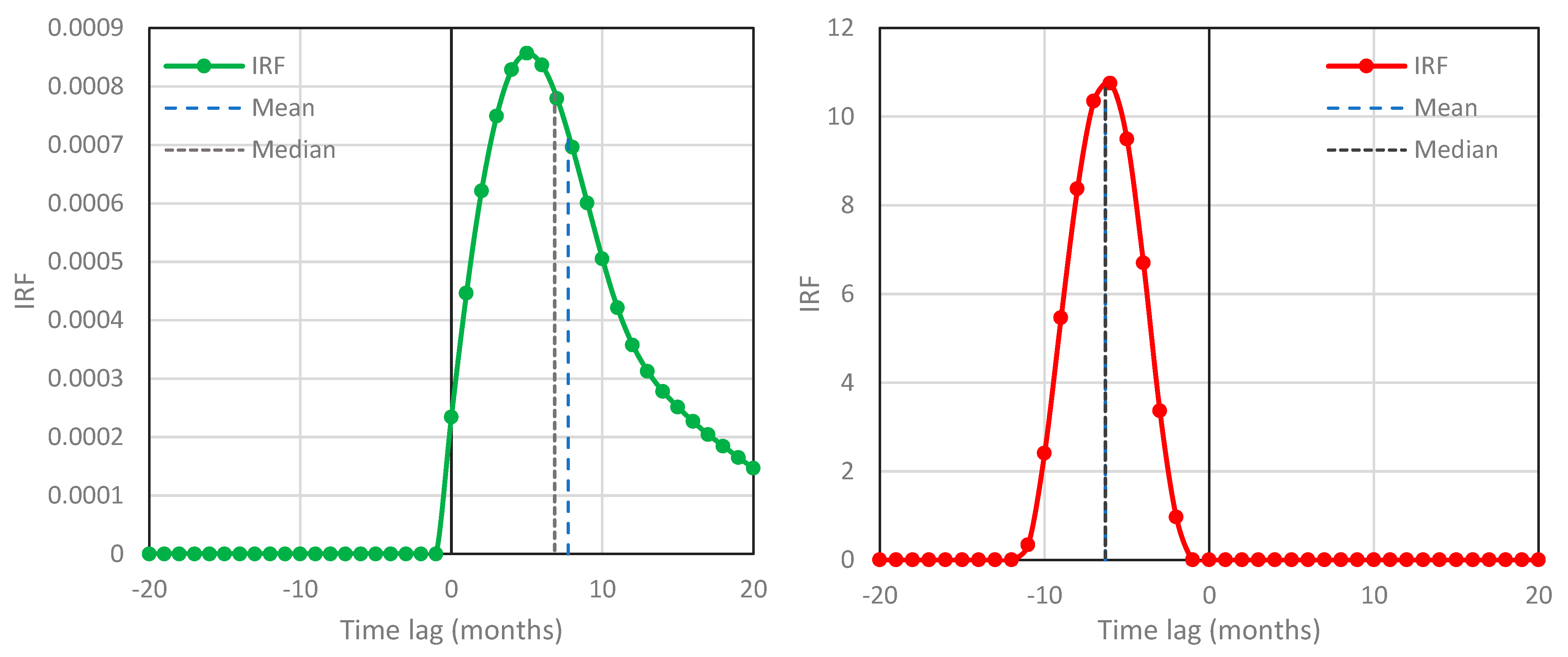
Appendix A.3. Investigation of Causality between El Niño, Atmospheric Temperature and CO2

A second process that is known to affect atmospheric temperature globally is the El Niño–Southern Oscillation (ENSO) (see [12,61] and a recent study by Kundzewicz et al. [62] for details). ENSO is associated with irregular variations in sea surface temperature and air pressure over the tropical Pacific Ocean. Several indices associated with ENSO are used in climatic studies, among which the most popular is US NOAA’s Southern Oscillation Index (SOI), the time series of which is plotted in Figure A5.
Figure A5. SOI time series (continuous line) along with rolling (right-aligned) 10-year average (dashed line). Negative and positive values indicate the El Niño and La Niña phases, respectively.
Sci 05 00035 g0a5
Our stochastic methodology was previously applied with SOI along with satellite temperature data for the period 1979–2021 in [7]. Here we repeat the investigation replacing the temperature data with those of the NCEP/NCAR reanalysis and expanding the data back to 1951 (the beginning of the availability of SOI data) and forth to 2022. We also examined the potential causality between SOI and [CO2]. In both cases, we tested differences with a time step of differencing of 1 year (thus reducing the effect of seasonality) and to make the correlation positive, we used Δ S O I (as in the albedo case).
The results are shown in Table A2, Figure A6 and Figure A7. The principal directions are S O I T and S O I [ C O 2 ] . In the former case, the explained variance is 33%, and the causality type is HOE but very close to unidirectional with a time lag of 4 months. In the latter case, the explained variance is 30%, and the causality type is unidirectional with a lag of about a year.
Table A2. Summary indices of the case studies related to ENSO. Data are on a monthly timescale and the time step of differencing is 1 year; for explanation of symbols see Table 1.
Case System#Direction h c μ h h 1 / 2 r y x h c e ε
S O I : NOAA; T: NCEP/NCAR;
period: 1951–2022
26 Δ S O I Δ T 34.143.850.460.338.1 × 10–4
27 Δ T Δ S O I 3–2.15–0.930.460.302.3 × 10–3
S O I : NOAA; [CO2]: Mauna Loa,
period: 1958–2022
28 Δ S O I Δ l n [ C O 2 ] 1111.6211.150.320.246.6 × 10–4
29 Δ l n C O 2 Δ S O I –11−3.73–3.840.320.080
Figure A6. IRFs for ENSO–temperature based on the SOI time series and the NCEP/NCAR Reanalysis temperature at 2 m, respectively—case studies #26 (left; Δ S O I Δ T ] ;) and #27 (right; Δ T Δ S O I ).
Sci 05 00035 g0a6
Figure A7. IRFs for ENSO–[CO2] based on the SOI and the Mauna Loa time series, respectively—case studies #28 (left; Δ S O I Δ l n [ C O 2 ] ] ;) and #29 (right; Δ l n C O 2 Δ S O I ).
Sci 05 00035 g0a7

Appendix A.4. Investigation of Causality between Ocean Heat Content, Atmospheric Temperature and CO2

A third process examined in connection to both T and [CO2] is the heat content of the upper-layer ocean. This is indirectly represented by data of the upper ocean mean temperature of the layer 0–100 m [63] (OMT0–100), also known as Vertically Averaged Temperature Anomaly (0–100 m layer) [64]. These are based on historical ocean temperature data, bathythermograph data and Argo data [65] and are made available at the timescale of three months by the National Oceanographic Data Center of the US NOAA [64], as well as by the ClimExp platform, which we used to download the data. The time series, starting in 1955, is plotted in Figure A8.
Figure A8. OMT0–100 time series (continuous line) along with rolling (right-aligned) 10-year average (dashed line).
Sci 05 00035 g0a8
The results of the stochastic analyses are shown in Table A3, Figure A9 and Figure A10. The principal directions are OMT0–100 T and OMT0–100 [ C O 2 ] and the causality type is HOE. In the former case, the explained variance is substantial, 53%, and the time lag is 3–7 months, depending on the metric used (nb., the time lags in Table A3 are given in 3-monthly steps). In the latter case, the explained variance is 35%, and the time lag is greater, 7–9 months.
Table A3. Summary indices of the case studies related to OMT0–100. Data are on a three-month timescale and the time step of differencing is 1 year; for explanation of symbols see Table 1.
Case System#Direction h c μ h h 1 / 2 r y x h c e ε
OMT0–100: NOAA; T: NCEP/NCAR; period: 1955–202230ΔOMT0–100 Δ T 02.420.980.680.537.1 × 10–3
31 Δ T ΔOMT0–1000–2.15–0.930.680.523.8 × 10–3
OMT0–100: NOAA; [CO2]: Mauna Loa; period: 1958–202232ΔOMT0–100 Δ l n [ C O 2 ] 22.222.930.460.355.8 × 10–4
33 Δ l n C O 2 ΔOMT0–100–2−2.73–2.820.460.215.6 × 10–3
Figure A9. IRFs for upper ocean temperature—atmospheric temperature based on the OMT0–100 and the NCEP/NCAR Reanalysis data, respectively—case studies #30 (left; ΔOMT0–100 Δ T ] ;) and #31 (right; Δ T ΔOMT0–100).
Sci 05 00035 g0a9
Figure A10. IRFs for upper ocean temperature—[CO2] based on the OMT0–100 and the NCEP/NCAR Reanalysis data, respectively—case studies #32 (left; ΔOMT0–100 Δ l n [ C O 2 ] ] ;) and #33 (right; Δ l n C O 2 ΔOMT0–100).
Sci 05 00035 g0a10

Appendix A.5. Notes on the T-[CO2] Relationship on Large Timescales

While the scope of this study is the modern period covered by reliable CO2 concentration measurements (about six decades), it may be useful to refer to studies that used paleoclimatic proxies to assess the T-[CO2] relationship on much larger timescales. Berner and Kothavala [66] studied the entire phanerozoic (the last 530 million years) and asserted that “over the long term there is indeed a correlation between CO2 and paleotemperature”, while their Figure 13 showed that the atmospheric [CO2] was much higher (up to 27 times) than the current one for most of the time during the phanerozoic. They also emphasized the “importance of considering ALL factors affecting CO2 when modelling the long term carbon cycle and not concentrating [on] only one cause”. On the other hand, Veizer et al. [67] presented evidence for decoupling atmospheric CO2 and global climate during the phanerozoic, questioning the role of the (partial pressure of) CO2 as the main driving force of past global (long-term) climate changes, at least during two of the four main cool climate modes of the phanerozoic.
Several studies, based on paleoclimatic reconstructions and mostly the Vostok ice cores [68,69] covering the most recent ~400 thousand years, have identified the change of T as the cause and that in [CO2] as the effect, with estimates of the time lag varying from 50 to 1000 years, depending on the time period and the particular study [23,70,71,72]. Claims that CO2 concentration leads (i.e., a negative lag) have not generally been made in these studies. At most, a synchrony claim has been sought on the basis that the estimated positive lags are often within the 95% uncertainty range [73], while in one of them [72], it has been asserted that a “short lead of CO2 over temperature cannot be excluded”.
Synchrony was also claimed for the last deglacial warming in another study by Parrenin et al. [74], who stated that they found no significant asynchrony between Antarctic temperature and atmospheric [CO2]. For the same period, another study by Shakun et al. [75] gave different lead-lag relationships for the north and south hemispheres. Generally, it appears that the issue remains controversial, as illustrated, for example, in a recent report (2021) by NOAA (in the framework of Paleo Perspectives [76]), which states: “While it might seem simple to determine cause and effect between carbon dioxide and climate from which change occurs first, […] the determination of cause and effect remains exceedingly difficult.”
On the other hand, a convincing explanation about why, in the long run, change in temperature leads and in CO2 concentration follows has been given by Roe [40], who demonstrated that in the Quaternary it is the effect of Milanković cycles, rather than of atmospheric CO2 concentration, that explains the glaciation process. Specifically, he found that “variations in atmospheric CO2 appear to lag the rate of change of global ice volume. This implies only a secondary role for CO2—variations in which produce a weaker radiative forcing than the orbitally-induced changes in summertime insolation—in driving changes in global ice volume.
The Vostok ice cores covering the most recent ~400 thousand years have also been examined, applying the same method as in this paper, by Koutsoyiannis et al. [7], who concluded that “the causal relationship of atmospheric T and CO2 concentration, as obtained by proxy data, appears to be of HOE type with principal direction T → [CO2]”, same as in the records of the modern period, but with a much higher time lag, of the order of 1000 years.

References

  1. Sagan, C. Cosmos; Ballantine Books: New York, NY, USA, 1985. [Google Scholar]
  2. Koutsoyiannis, D.; Kundzewicz, Z.W. Atmospheric temperature and CO2: Hen-or-egg causality? Sci 2020, 2, 83. [Google Scholar] [CrossRef]
  3. Πλούταρχος, Συμποσιακά Β’ (Plutarch, Quaestiones Convivales B’)—Βικιθήκη. Available online: https://el.wikisource.org/wiki/Συμποσιακά_Β΄ (accessed on 5 February 2023).
  4. Chan, K.H.; Hayya, J.C.; Ord, J.K. A note on trend removal methods: The case of polynomial regression versus variate differencing. Econometrica 1977, 45, 737–744. [Google Scholar] [CrossRef]
  5. Estrella, A. Why does the yield curve predict output and inflation? Econ. J. 2005, 115, 722–744. [Google Scholar] [CrossRef]
  6. Koutsoyiannis, D.; Onof, C.; Christofides, A.; Kundzewicz, Z.W. Revisiting causality using stochastics: 1. Theory. Proc. R. Soc. A 2022, 478, 20210836. [Google Scholar] [CrossRef]
  7. Koutsoyiannis, D.; Onof, C.; Christofides, A.; Kundzewicz, Z.W. Revisiting causality using stochastics: 2. Applications. Proc. R. Soc. A 2022, 478, 20210835. [Google Scholar] [CrossRef]
  8. Young, P.C. Recursive Estimation and Time Series Analysis; Springer: Berlin/Heidelberg, Germany, 2011. [Google Scholar]
  9. Young, P.C. Refined instrumental variable estimation: Maximum likelihood optimization of a unified Box-Jenkins model. Automatica 2015, 52, 35–46. [Google Scholar] [CrossRef]
  10. Papoulis, A. Probability, Random Variables and Stochastic Processes, 3rd ed.; McGraw-Hill: New York, NY, USA, 1991. [Google Scholar]
  11. Kestin, T.S.; Karoly, D.J.; Yang, J.I.; Rayner, N.A. Time-frequency variability of ENSO and stochastic simulations. J. Clim. 1998, 11, 2258–2272. [Google Scholar] [CrossRef]
  12. Wills, R.C.; Schneider, T.; Wallace, J.M.; Battisti, D.S.; Hartmann, D.L. Disentangling global warming, multidecadal variability, and El Niño in Pacific temperatures. Geophys. Res. Lett. 2018, 45, 2487–2496. [Google Scholar] [CrossRef]
  13. Granger, C.W. Investigating causal relations by econometric models and cross-spectral methods. Econometrica 1969, 37, 424–438. [Google Scholar] [CrossRef]
  14. Granger, C.W. Testing for causality: A personal viewpoint. J. Econ. Dyn. Control. 1980, 2, 329–352. [Google Scholar] [CrossRef]
  15. Moraffah, R.; Sheth, P.; Karami, M.; Bhattacharya, A.; Wang, Q.; Tahir, A.; Raglin, A.; Liu, H. Causal inference for time series analysis: Problems, methods and evaluation. Knowl. Inf. Syst. 2021, 63, 3041–3085. [Google Scholar] [CrossRef]
  16. Pearl, J. Causal inference in statistics: An overview. Stat. Surv. 2009, 3, 96–146. [Google Scholar] [CrossRef]
  17. Pearl, J.; Glymour, M.; Jewell, N.P. Causal Inference in Statistics: A Primer; Wiley: Chichester, UK, 2016. [Google Scholar]
  18. Pearl, J. and Mackenzie, D., The Book of Why, The New Science of Cause and Effect, Basic Books: New York, NY, USA, 2018.
  19. Kalnay, E.; Kanamitsu, M.; Kistler, R.; Collins, W.; Deaven, D.; Gandin, L.; Iredell, M.; Saha, S.; White, G.; Woollen, J.; et al. The NCEP/NCAR 40-year reanalysis project. Bull. Am. Meteorol. Soc. 1996, 77, 437–472. [Google Scholar] [CrossRef]
  20. Meinshausen, M.; Nicholls, Z.R.J.; Lewis, J.; Gidden, M.J.; Vogel, E.; Freund, M.; Beyerle, U.; Gessner, C.; Nauels, A.; Bauer, N.; et al. The shared socio-economic pathway (SSP) greenhouse gas concentrations and their extensions to 2500. Geosci. Model Dev. 2020, 13, 3571–3605. [Google Scholar] [CrossRef]
  21. Sellar, A.A.; Jones, C.G.; Mulcahy, J.P.; Tang, Y.; Yool, A.; Wiltshire, A.; O’Connor, F.M.; Stringer, M.; Hill, R.; Palmieri, J.; et al. UKESM1: Description and evaluation of the UK Earth System Model. J. Adv. Model. Earth Syst. 2019, 11, 4513–4558. [Google Scholar] [CrossRef]
  22. Koutsoyiannis, D. Stochastics of Hydroclimatic Extremes—A Cool Look at Risk, 2nd ed.; Kallipos Open Academic Editions: Athens, Greece, 2022; 346p, ISBN 978-618-85370-0-2. [Google Scholar] [CrossRef]
  23. Koutsoyiannis, D. Time’s arrow in stochastic characterization and simulation of atmospheric and hydrological processes. Hydrol. Sci. J. 2019, 64, 1013–1037. [Google Scholar] [CrossRef]
  24. Strotz, R.H.; Wold, H.O.A. Recursive vs. nonrecursive systems: An attempt at synthesis (Part I of a triptych on causal chain systems). Econometrica 1960, 28, 417–427. Available online: https://www.jstor.org/stable/1907731 (accessed on 15 March 2023). [CrossRef]
  25. Hannart, A.; Pearl, J.; Otto, F.E.L.; Naveau, P.; Ghil, M. Causal counterfactual theory for the attribution of weather and climate-related events. Bull. Am. Met. Soc. 2016, 97, 99–110. [Google Scholar] [CrossRef]
  26. Hannart, A.; Naveau, P. Probabilities of causation of climate changes. J. Clim. 2018, 31, 5507–5524. [Google Scholar] [CrossRef]
  27. Koutsoyiannis, D.; Efstratiadis, A.; Mamassis, N.; Christofides, A. On the credibility of climate predictions. Hydrol. Sci. J. 2008, 53, 671–684. [Google Scholar] [CrossRef]
  28. Anagnostopoulos, G.G.; Koutsoyiannis, D.; Christofides, A.; Efstratiadis, A.; Mamassis, N. A comparison of local and aggregated climate model outputs with observed data. Hydrol. Sci. J. 2010, 55, 1094–1110. [Google Scholar] [CrossRef]
  29. Koutsoyiannis, D.; Christofides, A.; Efstratiadis, A.; Anagnostopoulos, G.G.; Mamassis, N. Scientific dialogue on climate: Is it giving black eyes or opening closed eyes? Reply to “A black eye for the Hydrological Sciences Journal” by D. Huard. Hydrol. Sci. J. 2011, 56, 1334–1339. [Google Scholar] [CrossRef]
  30. Tyralis, H.; Koutsoyiannis, D. On the prediction of persistent processes using the output of deterministic models. Hydrol. Sci. J. 2017, 62, 2083–2102. [Google Scholar] [CrossRef]
  31. Scafetta, N. CMIP6 GCM validation based on ECS and TCR ranking for 21st century temperature projections and risk assessment. Atmosphere 2023, 14, 345. [Google Scholar] [CrossRef]
  32. Masson-Delmotte, V.; Zhai, P.; Pirani, A.; Connors, S.L.; Péan, C.; Berger, S.; Caud, N.; Chen, Y.; Goldfarb, L.; Gomis, M.I.; et al. (Eds.) IPCC, Climate Change 2021: The Physical Science Basis. Contribution of Working Group I to the Sixth Assessment Report of the Intergovernmental Panel on Climate Change; Cambridge University Press: Cambridge, UK; New York, NY, USA, 2021; 2391p. [Google Scholar] [CrossRef]
  33. Koutsoyiannis, D. Rethinking climate, climate change, and their relationship with water. Water 2021, 13, 849. [Google Scholar] [CrossRef]
  34. Zhu, Z.; Piao, S.; Myneni, R.B.; Huang, M.; Zeng, Z.; Canadell, J.G.; Ciais, P.; Sitch, S.; Friedlingstein, P.; Arneth, A.; et al. Greening of the Earth and its drivers. Nature Climate Change 2016, 6, 791–795. [Google Scholar] [CrossRef]
  35. Li, Y.; Li, Z.L.; Wu, H.; Zhou, C.; Liu, X.; Leng, P.; Yang, P.; Wu, W.; Tang, R.; Shang, G.F.; et al. Biophysical impacts of earth greening can substantially mitigate regional land surface temperature warming. Nat. Commun. 2023, 14, 121. [Google Scholar] [CrossRef]
  36. Chen, C.; Park, T.; Wang, X.; Piao, S.; Xu, B.; Chaturvedi, R.K.; Fuchs, R.; Brovkin, V.; Ciais, P.; Fensholt, R.; et al. China and India lead in greening of the world through land-use management. Nat. Sustain. 2019, 2, 122–129. [Google Scholar] [CrossRef]
  37. Milanković, M. Nebeska Mehanika; Udruženje “Milutin Milanković”: Beograd, Serbia, 1935. [Google Scholar]
  38. Milanković, M. Kanon der Erdbestrahlung und Seine Anwendung auf das Eiszeitenproblem; Koniglich Serbische Akademice: Beograd, Serbia, 1941. [Google Scholar]
  39. Milanković, M. Canon of Insolation and the Ice-Age Problem; Agency for Textbooks: Belgrade, Serbia, 1998. [Google Scholar]
  40. Roe, G. In defense of Milankovitch. Geophys. Res. Lett. 2006, 33, L24703. [Google Scholar] [CrossRef]
  41. Markonis, Y.; Koutsoyiannis, D. Climatic variability over time scales spanning nine orders of magnitude: Connecting Milankovitch cycles with Hurst–Kolmogorov dynamics. Surv. Geophys. 2013, 34, 181–207. [Google Scholar] [CrossRef]
  42. Stephens, G.L.; Hakuba, M.Z.; Kato, S.; Gettelman, A.; Dufresne, J.-L.; Andrews, T.; Cole, J.N.S.; Willen, U.; Mauritsen, T. The changing nature of Earth’s reflected sunlight. Proc. R. Soc. A 2022, 478, 1–37. [Google Scholar] [CrossRef]
  43. Connolly, R.; Soon, W.; Connolly, M.; Baliunas, S.; Berglund, J.; Butler, C.J.; Cionco, R.G.; Elias, A.G.; Fedorov, V.M.; Harde, H.; et al. How much has the Sun influenced Northern Hemisphere temperature trends? An ongoing debate. Res. Astron. Astrophys. 2021, 21, 131.1–131.68. [Google Scholar] [CrossRef]
  44. Scafetta, N.; Bianchini, A. The planetary theory of solar activity variability: A review. Front. Astron. Space Sci. 2022, 9, 937930. [Google Scholar] [CrossRef]
  45. Kamis, J.E. The Plate Climatology Theory: How Geological Forces Influence, Alter, or Control Earth’s Climate and Climate Related Events. Available online: https://books.google.gr/books/?id=7lRqzgEACAAJ (accessed on 10 March 2023).
  46. Chakrabarty, D. The Climate of History in a Planetary Age; University of Chicago Press: Chicago, IL, USA, 2021; Available online: https://books.google.gr/books?id=ETQXEAAAQBAJ (accessed on 10 March 2023).
  47. Davis, E.; Becker, K.; Dziak, R.; Cassidy, J.; Wang, K.; Lilley, M. Hydrological response to a seafloor spreading episode on the Juan de Fuca ridge. Nature 2004, 430, 335–338. [Google Scholar] [CrossRef] [PubMed]
  48. Urakawa, L.S.; Hasumi, H. A remote effect of geothermal heat on the global thermohaline circulation. J. Geophys. Res. Ocean. 2009, 114, C07016. [Google Scholar] [CrossRef]
  49. Patara, L.; Böning, C.W. Abyssal ocean warming around Antarctica strengthens the Atlantic overturning circulation. Geophys. Res. Lett. 2014, 41, 3972–3978. [Google Scholar] [CrossRef]
  50. Koutsoyiannis, D. A random walk on water. Hydrol. Earth Syst. Sci. 2010, 14, 585–601. [Google Scholar] [CrossRef]
  51. Koutsoyiannis, D. Hydrology and change. Hydrol. Sci. J. 2013, 58, 1177–1197. [Google Scholar] [CrossRef]
  52. Friedlingstein, P.; O’Sullivan, M.; Jones, M.W.; Andrew, R.M.; Gregor, L.; Hauck, J.; Le Quéré, C.; Luijkx, I.T.; Olsen, A.; Peters, G.P.; et al. Global Carbon Budget 2022. Earth Syst. Sci. Data 2022, 14, 4811–4900. [Google Scholar] [CrossRef]
  53. Stallinga, P. Residence time vs. adjustment time of carbon dioxide in the atmosphere. Entropy 2023, 25, 384. [Google Scholar] [CrossRef]
  54. Hansen, J.E.; Sato, M.; Simons, L.; Nazarenko, L.S.; von Schuckmann, K.; Loeb, N.G.; Osman, M.B.; Kharecha, P.; Jin, Q.; Tselioudis, G.; et al. Global warming in the pipeline. arXiv 2022, arXiv:2212.04474. [Google Scholar]
  55. Bond-Lamberty, B.; Thomson, A. Temperature-associated increases in the global soil respiration record. Nature 2010, 464, 579. [Google Scholar] [CrossRef] [PubMed]
  56. Arrhenius, S.A. Über die Dissociationswärme und den Einfluß der Temperatur auf den Dissociationsgrad der Elektrolyte. Z. Phys. Chem. 1889, 4, 96–116. [Google Scholar] [CrossRef]
  57. Patel, K.F.; Bond-Lamberty, B.; Jian, J.L.; Morris, K.A.; McKever, S.A.; Norris, C.G.; Zheng, J.; Bailey, V.L. Carbon flux estimates are sensitive to data source: A comparison of field and lab temperature sensitivity data. Environ. Res. Lett. 2022, 17, 113003. [Google Scholar] [CrossRef]
  58. Pomeroy, R.; Bowlus, F.D. Progress report on sulfide control research. Sew. Work. J. 1946, 18, 597–640. [Google Scholar]
  59. Robinson, C. Microbial respiration, the engine of ocean deoxygenation. Front. Mar. Sci. 2019, 5, 533. [Google Scholar] [CrossRef]
  60. CERES Data Products. SSF1deg—Level 3, Gridded Daily and Monthly Averages of the SSF Product by Instrument. Available online: https://ceres-tool.larc.nasa.gov/ord-tool/jsp/SSF1degEd41Selection.jsp (accessed on 12 March 2023).
  61. McPhaden, M.J.; Zebiak, S.E.; Glantz, M.H. ENSO as an integrating concept in earth science. Science 2006, 314, 1740–1745. [Google Scholar] [CrossRef]
  62. Kundzewicz, Z.W.; Pinskwar, I.; Koutsoyiannis, D. Variability of global mean annual temperature is significantly influenced by the rhythm of ocean-atmosphere oscillations. Sci. Total Environ. 2020, 747, 141256. [Google Scholar] [CrossRef]
  63. Levitus, S.; Antonov, J.I.; Boyer, T.P.; Baranova, O.K.; Garcia, H.E.; Locarnini, R.A.; Mishonov, A.V.; Reagan, J.R.; Seidov, D.; Yarosh, E.S.; et al. World Ocean heat content and thermosteric sea level change (0–2000 m). Geophys. Res. Lett. 2012, 39, L10603. [Google Scholar] [CrossRef]
  64. National Oceanographic Data Center, NOAA, Global Ocean Heat and Salt Content. Available online: https://www.ncei.noaa.gov/access/global-ocean-heat-content/index3.html (accessed on 12 March 2023).
  65. Roemmich, D.; Johnson, G.C.; Riser, S.; Davis, R.; Gilson, J.; Owens, W.B.; Garzoli, S.L.; Schmid, C.; Ignaszewski, M. The Argo Program: Observing the global ocean with profiling floats. Oceanography 2009, 22, 34–43. [Google Scholar] [CrossRef]
  66. Berner, R.A.; Kothavala, Z. GEOCARB III: A revised model of atmospheric CO2 over Phanerozoic time. Am. J. Sci. 2001, 301, 182–204. [Google Scholar] [CrossRef]
  67. Veizer, J.; Godderis, Y.; François, L.M. Evidence for decoupling of atmospheric CO2 and global climate during the Phanerozoic eon. Nature 2000, 408, 698–701. [Google Scholar] [CrossRef] [PubMed]
  68. Jouzel, J.; Lorius, C.; Petit, J.R.; Genthon, C.; Barkov, N.I.; Kotlyakov, V.M.; Petrov, V.M. Vostok ice core: A continuous isotope temperature record over the last climatic cycle (160,000 years). Nature 1987, 329, 403–408. [Google Scholar] [CrossRef]
  69. Petit, J.R.; Jouzel, J.; Raynaud, D.; Barkov, N.I.; Barnola, J.-M.; Basile, I.; Bender, M.; Chappellaz, J.; Davis, M.; Delayque, G.; et al. Climate and atmospheric history of the past 420,000 years from the Vostok ice core, Antarctica. Nature 1999, 399, 429–436. [Google Scholar] [CrossRef]
  70. Caillon, N.; Severinghaus, J.P.; Jouzel, J.; Barnola, J.M.; Kang, J.; Lipenkov, V.Y. Timing of atmospheric CO2 and Antarctic temperature changes across Termination III. Science 2003, 299, 1728–1731. [Google Scholar] [CrossRef]
  71. Soon, W. Implications of the secondary role of carbon dioxide and methane forcing in climate change: Past, present, and future. Phys. Geogr. 2007, 28, 97–125. [Google Scholar] [CrossRef]
  72. Pedro, J.B.; Rasmussen, S.O.; van Ommen, T.D. Tightened constraints on the time-lag between Antarctic temperature and CO2 during the last deglaciation. Clim. Past 2012, 8, 1213–1221. [Google Scholar] [CrossRef]
  73. Chowdhry Beeman, J.; Gest, L.; Parrenin, F.; Raynaud, D.; Fudge, T.J.; Buizert, C.; Brook, E.J. Antarctic temperature and CO2: Near-synchrony yet variable phasing during the last deglaciation. Clim. Past 2019, 15, 913–926. [Google Scholar] [CrossRef]
  74. Parrenin, F.; Masson-Delmotte, V.; Köhler, P.; Raynaud, D.; Paillard, D.; Schwander, J.; Barbante, C.; Landais, A.; Wegner, A.; Jouzel, J. Synchronous change of atmospheric CO2 and Antarctic temperature during the last deglacial warming. Science 2013, 339, 1060–1063. [Google Scholar] [CrossRef]
  75. Shakun, J.D.; Clark, P.U.; He, F.; Marcott, S.A.; Mix, A.C.; Liu, Z.; Otto-Bliesner, B.; Schmittner, A.; Bard, E. Global warming preceded by increasing carbon dioxide concentrations during the last deglaciation. Nature 2012, 484, 49–54. [Google Scholar] [CrossRef]
  76. NOAA National Centers for Environmental Information. Temperature Change and Carbon Dioxide Change; 2021. Available online: https://www.ncei.noaa.gov/sites/default/files/2021-11/8%20-%20Temperature%20Change%20and%20Carbon%20Dioxide%20Change%20-%20FINAL%20OCT%202021.pdf (accessed on 12 January 2023).
Figure 1. Explanatory sketch for the definition of the different potential causality types. For each graph, the mean μ h is also plotted with a dashed line.
Sci 05 00035 g001
Figure 2. IRFs for temperature–CO2 concentration based on the NCEP/NCAR Reanalysis temperature at 2 m and Mauna Loa [CO2] time series, respectively—case studies #3 (left; Δ T Δ l n [ C O 2 ] ; potentially causal system) and #4 (right; Δ l n [ C O 2 ] Δ T ; potentially anticausal system).
Sci 05 00035 g002
Figure 3. IRFs for temperature–CO2 concentration based on the NCEP/NCAR Reanalysis temperature at 2 m and the South Pole time series, respectively—case studies #14 (left; Δ T Δ l n [ C O 2 ] ; potentially causal system) and #15 (right; Δ l n [ C O 2 ] Δ T ; potentially anticausal system).
Sci 05 00035 g003
Figure 4. (Left column) Empirical autocorrelation function for the period 1958–2021 and for monthly timescale of (upper) the NCEP/NCAR Δ T time series and (lower) the Δ l n [ C O 2 ] time series for Mauna Loa. (Right column) Empirical cross-correlation function of the two time series (continuous lines in blue), compared with those reconstructed from the IRF and the autocorrelation function on the left panel using the discretized version of Equation (7) (dashed line), for case studies (upper) #3 and (lower) #4.
Sci 05 00035 g004
Figure 5. IRFs for temperature–CO2 concentration based on the NCEP/NCAR Reanalysis temperature at 2 m and Mauna Loa time series, respectively, as in Figure 2, but for differencing time steps equal (from upper to lower) 2, 4, 8 and 16 years; left: Δ T Δ l n [ C O 2 ] (potentially causal system); right: Δ l n [ C O 2 ] Δ T (potentially anticausal system).
Sci 05 00035 g005aSci 05 00035 g005b
Figure 6. IRFs for temperature–CO2 concentration based on the NCEP/NCAR Reanalysis temperature at 2 m and Mauna Loa time series, respectively, also enabling negative lags (HOE) for causality direction Δ T Δ l n [ C O 2 ] and for differencing time step of 1 year (left, corresponding to Figure 2, left) and 16 years (right, corresponding to Figure 5, bottom left).
Sci 05 00035 g006
Figure 7. IRFs for temperature–CO2 concentration based on the NCEP/NCAR Reanalysis temperature at 2 m and Mauna Loa time series, for 21 time lags, differencing time step of 16 years and direction Δ T Δ l n [ C O 2 ] . The lowest nonzero lag of each IRF is marked at the upper-right end of its curve.
Sci 05 00035 g007
Figure 8. Explained variance and median of IRF as a function of the lowest nonzero lag of the IRFs in Figure 7 for the investigation of Section 7.
Sci 05 00035 g008
Figure 9. IRFs for temperature–CO2 concentration based on the CMIP6 mean temperature and SSP2-4.5 CO2 time series, respectively, calculated without using the roughness constraint; upper row: period 1850–2100—case studies #16 (left; Δ T Δ l n [ C O 2 ] ) and #17 (right; Δ l n [ C O 2 ] Δ T ); lower row: period 1850–2021—case studies #18 (left; Δ T Δ l n [ C O 2 ] ) and #19 (right; Δ l n [ C O 2 ] Δ T ).
Sci 05 00035 g009
Figure 10. IRFs for temperature–CO2 concentration based on the CMIP6 mean temperature and SSP2-4.5 CO2 time series, respectively, as in Figure 9 but calculated using the roughness constraint; upper row: period 1850–2100—case studies #20 (left; Δ T Δ l n [ C O 2 ] ) and #21 (right; Δ l n [ C O 2 ] Δ T ); lower row: period 1850–2021—case studies #22 (left; Δ T Δ l n [ C O 2 ] ) and #23 (right; Δ l n [ C O 2 ] Δ T ).
Sci 05 00035 g010
Figure 11. Empirical cross-correlation functions for monthly and annual timescales (continuous lines in blue without markers and red lines with circles, respectively) for the data sets indicated in each panel. In all panels, the plot for the monthly scale is that of the NCEP/NCAR data for T and Mauna Loa data for [CO2], for the period 1958–2021. The upper-left panel also shows the cross-correlation function reconstructed from the IRF and the autocorrelation function using the discretized version of Equation (7) (dashed line).
Sci 05 00035 g011
Figure 12. Empirical autocorrelation functions for monthly and annual timescales (continuous lines in blue without markers and red lines with circles, respectively) for the data sets indicated in each panel. In all panels, the plot for the monthly scale is that of the NCEP/NCAR data for T and Mauna Loa data for [CO2], for the period 1958–2021.
Sci 05 00035 g012
Figure 13. Schematic of the examined possible causal links in the climatic system, with noted types of potential causality, HOE or unidirectional, and its direction. Other processes, not examined here, could be internal of the climatic system or external.
Sci 05 00035 g013
Figure 14. Modified IRF for temperature–CO2 concentration based on the NCEP/NCAR Reanalysis temperature at 2 m and Mauna Loa time series, respectively, similar to Figure 2 but with IRF coordinates simultaneously optimized with the parameters of Equation (9).
Sci 05 00035 g014
Figure 15. Comparison of the actual Δ l n [ C O 2 ] (upper) and [ C O 2 ] (lower) with those simulated by the model of Equations (8) and (9).
Sci 05 00035 g015
Table 1. Main case studies and resulting summary indices. Δ t is the time step of differencing; h c is the time lag maximizing the cross-covariance c y x h , or equivalently the cross-correlation r y x h   : = c y x h / c x x 0 c y y 0 ; μ h is the mean (time average) of the function   g ( h ) ; h 1 / 2 is the median of the function   g ( h ) ; e is the explained variance ratio; and ε is the roughness ratio. The case studies #1 and #2 are contained in [7] as case studies #23 and #24 and are included in the table only for comparison.
Case System#Direction h c μ h h 1 / 2 r y x h c e ε
Monthly timescale, varying Δt
T :   UAH ;   [ CO 2 ] :   Mauna   Loa ,   1979 2020   ( from   [ 7 ] ) ,   Δ t = 1 year 1 Δ T Δ l n [ C O 2 ] 57.706.350.480.311.3 × 10–5 *
2 Δ l n [ C O 2 ] Δ T –5–5.67–5.490.480.237.3 × 10–4 *
T :   NCEP / NCAR ;   [ CO 2 ] :   Mauna   Loa ,   1958 2021 ,   Δ t = 1 year3 Δ T Δ l n [ C O 2 ] 87.756.860.560.343.1 × 10–4 *
4 Δ l n [ C O 2 ] Δ T –8−6.31–6.300.560.234.4 × 10–3 *
As   # 3   and   # 4 ,   Δ t = 2 years5 Δ T Δ l n [ C O 2 ] 88.197.080.570.313.4 × 10–4 *
6 Δ l n [ C O 2 ] Δ T –8−6.31–6.310.570.214.5 × 10–3 *
As   # 3   and   # 4 ,   Δ t = 4 years7 Δ T Δ l n [ C O 2 ] 910.6510.320.530.291.0 × 10–4 *
8 Δ l n [ C O 2 ] Δ T –9−6.28–6.280.530.143.8 × 10–3 *
As   # 3   and   # 4 ,   Δ t = 8 years9 Δ T Δ l n [ C O 2 ] 811.0011.000.470.275.6 × 10–5 *
10 Δ l n [ C O 2 ] Δ T –8−6.55–6.540.470.113.6 × 10–3 *
As   # 3   and   # 4 ,   Δ t = 16 years11 Δ T Δ l n [ C O 2 ] 611.7412.150.450.313.4 × 10–5 *
12 Δ T Δ l n [ C O 2 ] 69.9811.130.450.337.6 × 10–6
13 Δ l n [ C O 2 ] Δ T –6−6.33–6.310.450.127.7 × 10–3 *
T :   NCEP / NCAR ;   [ CO 2 ] :   South   Pole ,   1975 2021 ,   Δ t = 1 year14 Δ T Δ l n [ C O 2 ] 109.768.910.400.352.0 × 10–4 *
15 Δ l n [ C O 2 ] Δ T –10–8.51–8.350.400.181.1 × 10–3 *
Annual timescale, Δ t = 1 year
T: CMIP6 mean, SSP2-4.5; [CO2]: SSP2-4.5, 1850–2100, w/o roughness constraint16 Δ T Δ l n [ C O 2 ] 0–3.75–6.200.360.900.095
17 Δ l n [ C O 2 ] Δ T 09.9515.300.360.150.46
As #16 and #17 but for 1850–202118 Δ T Δ l n [ C O 2 ] 0–6.23–8.580.310.720.10
19 Δ l n [ C O 2 ] Δ T 016.1816.160.310.100.295
As #16 and #17 but with roughness constraint20 Δ T Δ l n [ C O 2 ] 0–3.65–5.550.360.843.5 × 10–5
21 Δ l n [ C O 2 ] Δ T 06.861.630.360.137.7 × 10–3
As #18 and #19 but with roughness constraint22 Δ T Δ l n [ C O 2 ] 0–7.34–8.990.310.648.3 × 10–5
23 Δ l n [ C O 2 ] Δ T 011.2614.770.310.139.4 × 10–3
* The roughness was calculated without considering the second derivative at zero.
Disclaimer/Publisher’s Note: The statements, opinions and data contained in all publications are solely those of the individual author(s) and contributor(s) and not of MDPI and/or the editor(s). MDPI and/or the editor(s) disclaim responsibility for any injury to people or property resulting from any ideas, methods, instructions or products referred to in the content.

