Article

Methodology for Assessing the Technical Condition and Durability of Bridge Structures

by
Kostiantyn Medvediev
1,†,
Anna Kharchenko
1,†,
Anzhelika Stakhova
2,*,†,
Yurii Yevseichyk
1,†,
Vitalii Tsybulskyi
1,† and
Adrián Bekö
2,†
1
Faculty of Transport Construction, National Transport University, Omelyanovicha-Pavlenko str., 1, 01010 Kyiv, Ukraine
2
Department of Structural Mechanics, Faculty of Civil Engineering, Slovak University of Technology in Bratislava, Radlinského 11, SK-810 05 Bratislava, Slovakia
*
Author to whom correspondence should be addressed.
These authors contributed equally to this work.
Infrastructures 2024, 9(1), 16; https://doi.org/10.3390/infrastructures9010016
Submission received: 1 December 2023 / Revised: 14 January 2024 / Accepted: 15 January 2024 / Published: 22 January 2024

Abstract

:
The proposed methodology aims to determine and forecast the technical condition of bridge elements, which could serve as an advanced engineering tool for assessing reliability and durability. It is developed based on fundamental studies that synthesize the experience of studying the physical–mechanical and physical–chemical properties of materials in bridge structures operating under real conditions. The theoretical foundation of the methodology is a reliability model and residual lifetime prediction of bridge elements based on Markov’s theory. The developed methodology is designed for assessing the technical condition of individual bridge elements, followed by a comprehensive evaluation of the entire structure. Reliability during operation is adopted as the indicator of technical condition. This quantitative reliability indicator in the model serves as a criterion for evaluating the safety level of bridge elements; ranking of bridge elements as necessary for specific types of repair, reconstruction, or replacement; strategic planning of expenditures for repair or reconstruction under limited funding; and forecasting the remaining resource of elements. An evaluation and prediction algorithm for the technical condition of bridges is proposed for the application of the developed methodology. A mathematical experiment of the developed methodology was conducted, which confirmed the adequacy of the proposed hypothesis, i.e., the use of the reliability model and the prediction of residual lifetime of bridge elements. First, a three-step mechanism for refining the technical condition of the bridge is proposed, significantly enhancing the accuracy of the calculations. Therefore, the developed methodology holds practical value and can serve as a basis for information-analytical systems for managing the condition of bridges.

1. Introduction

The assessment of the technical condition of bridges is a crucial aspect of effective operational maintenance management. Inadequate maintenance of bridge elements affects the overall structure’s durability. The performance and operational characteristics of bridges deteriorate over time, and they are constantly subjected to the aggressive influence of the environment (humidity, temperature, and wind erosion), mechanical damage during winter maintenance, increased traffic intensity, and higher demands for load capacity [1]. This necessitates continuous monitoring of the state of bridges, as well as forecasting the residual capacity to take preventive actions for structure preservation. Thus, the theoretical approaches to testing bridges with subsequent diagnosis of their technical condition, taking into account the structural state and assessing their overall condition, were analyzed in this study.
In studies [1,2], the experience of managing the condition of bridges based on degradation models using information-analytical bridge management systems has been analyzed. It is emphasized that the accuracy of the decisions made, significantly depends on the model for predicting the bridge’s residual lifetime. The most common types of models used as the basis for bridge management information systems were deterministic or stochastic. However, the authors of [3] have determined that mathematical formulations to describe degradation processes often have high complexity, so practical degradation models frequently rely solely on inspection results. The authors of [1,2] also emphasized that these models had inaccuracies in calculating the reliability of structural elements when determining the operational condition of bridges.
Reliability is one of the most important requirements for structures as outlined in the Eurocodes [4]. Therefore, it is crucial to ensure that the parameters of safety level, suitability for operation, and durability correspond to this indicator. In the study [5], a critical overview of models for calculating and predicting the technical condition of bridges based on the reliability parameter is provided. It is emphasized that most models are based on determining reliability for elements with a standard set of constructions and materials. The authors of [5] propose a hybrid calculation model that combines a modified process of fuzzy analytical hierarchy analysis (EA FAHP) and dominant analytical hierarchy process (DAHP). However, the authors note the complexity of calculations using their developed model for practicing engineers.
The practical significance of using reliability theory is elucidated in the work [6], using the example of testing concrete sleepers. Specifically, first-order and second-order reliability methods (FORM and SORM) in combination with the Monte Carlo simulation method were employed. Monte Carlo simulation was used to obtain variations in reliability over the service life of the structure. However, the results of the study [6] were limited to concrete sleepers and cannot be fully extrapolated to more complex structures such as bridges in our case.
In the work [5], it is proposed to use a mathematical framework based on fuzzy logic and transition intensity from one state of the bridge to another to determine the technical condition of the bridge. The rating of the bridge condition is achieved by summing the products of all component ratings by their relative importance.
By using degradation models, a deterministic value of the averaged predicted state of the bridge can be obtained. In research and in practice in several countries, deterministic methods of condition assessment are used, such as linear extrapolation, linear, non-linear, and stepwise regression, as well as methods based on degradation curves [7,8]. However, these methods do not take into account historical data on the changes in the condition of bridge elements. Thus, they can only be applied to short-term degradation forecasting [2].
In the contribution [9], the application of stochastic models is investigated, considering the degradation of bridge elements as a probabilistic process accompanied by uncertainty and randomness. The most commonly used stochastic models for predicting the degradation of infrastructure objects are considered to be Markov models, which are used in the majority of information-analytical bridge management systems in various countries [2,10]. It is believed that the advantage of using Markov models is the ability to forecast the condition of a structure based on available information from at least two visual inspections. In other words, these models operate on the assumption that the probability of the future state of the structure depends solely on its current technical condition. In particular, studies [11,12] consider the fundamental and applied aspects of applying Markov theory. The research demonstrates that even minor preventive maintenance of industrial objects influences the reduction in the acceleration of their elements’ degradation. However, the authors [11,12] consider that the methodology they developed for applying the Markov process is not perfect and requires improvement by relaxing the assumption of exponential sojourn times. The first Markov degradation model in Ukraine was proposed by Prof. A.I. Lantukh-Lyashchenko in 1999 [13]. Subsequently, the model was further developed and improved in works [14,15] and was verified in practical applications as an updated normative model for assessing and predicting the technical condition of bridge elements [16]. In the practices of Slovakia and the Czech Republic, a combined approach based on several models is used in the standards for assessing and predicting the condition of bridges [17].
ISO 15686 [18] describes the factorial method, defined as a tool for improving the assessment of the service life of a structure. The method uses modified coefficients for each group of factors from A to G (quality of components; design level; work execution level; indoor environment; outdoor environment; in-use conditions; and maintenance level). It is considered that any of these variables or their combination may affect the service life of the entire structure. However, there are studies that determine that the realistic range of coefficients is significant. Thus, users of the ISO 15686 methodology may not be able to select appropriate values for the coefficients without deep knowledge of materials and local construction practices [19], which are limitations in the application of the factorial method.
However, despite the recognition of these models as the most effective for predicting the condition of structures, it is considered that existing information-analytical systems based on these models in various countries have a number of drawbacks [2]. In particular, this includes the failure to account for the overall service life of the bridge in determining the transition probability from one state to the next [20]. Kleiner [21] proposed using probability distributions with increasing failure rates for an indefinite time of the structure being present in each conditional state. This underscores the issue of accelerating the degradation of bridge elements at higher operational states. Thus, there is a problem of determining the probability of transitioning to the next state for bridges of different service lives.
Another issue is the non-uniformity of obtaining actual data from inspections or measurements of technical indicators of bridge elements. In the study [2], it is emphasized that the determined operational state is not an accurate indicator of safety and suitability for use of the structure. Therefore, it is considered impossible to achieve precision in determining the state of the bridge solely based on the data from inspecting its elements.
In the field of bridge engineering, separate developments have been made in models based on the use of artificial intelligence, Bayesian networks (BN), Petri-Net (PN) models, and others. These models were developed as an attempt to overcome some limitations of existing traditional models [2].
Thus, the models and methods for assessing and predicting the technical condition of bridges identified in the studies [1,2,3,4,5,7,8,9,10,13,14,15,16,17,20,21] are not perfect, have limitations in their application, and require refinement. Additionally, the analysis of these studies has shown that adequate results cannot be obtained using traditional models. However, the significant attention of researchers to this problem confirms the relevance of the proposed research direction.
Based on the theory of the process of assessing the technical condition of bridges we develop a methodology for determining the technical condition and durability indefinite in terms of residual lifetime of bridge structures (Figure 1).

2. Materials and Methods

The main goal of inspecting bridge structures is to determine their technical condition and operational mode, as well as to assess their ability to withstand the designed loads, considering any detected defects. The results of the inspection provide conclusions regarding the current state of the bridge, its load-bearing capacity, the parameters of temporary loading, which the structure can withstand. This information is crucial for making decisions about repair or reconstruction.
To formalize the inspection process, Ukrainian regulatory documents [16] consider a bridge structure as a system consisting of seven groups of structural elements: span elements, supports and bearing parts, foundations, roadway elements, approaches, substructure elements, and accessories. The categorization of bridge elements into these groups takes into account their functional characteristics, allowing for the determination of the significance of each element for the subsequent trouble-free operation of the structure. It is worth noting that these groups of elements are subjected to various force factors, have different functions, service life, and influence on the overall structural stability.
The analysis of the inspection materials allows for the assessment of the technical condition of each group of bridge elements, enabling the determination of the operational state of the element group and the bridge structure as a whole. The basis for categorizing a bridge element into a particular operational state is based on data obtained through the analysis of the bridge’s primary technical documentation, operational records, examination of the operational history, detailed inspection of the entire structure and its elements, assessment of material strength at the time of inspection, load-bearing capacity verification, and determination of the actual safety characteristics of the elements, as well as conducting load tests if necessary.
In this research, bridges are considered as systems consisting of seven groups of structural elements. Subsequently, the technical condition of these elements is assessed by classifying them into one of the five accepted operational states (see Table 1). The classification is based on data collected during inspections and is regulated by normative documents (e.g., [16]), including:
  • Primary technical documentation of the bridge;
  • Operational documentation data;
  • Analysis of the operational history;
  • Detailed inspection data of the entire structure and its elements;
  • Determination of the actual material strength of the structural elements;
  • Bridge testing data (if necessary).
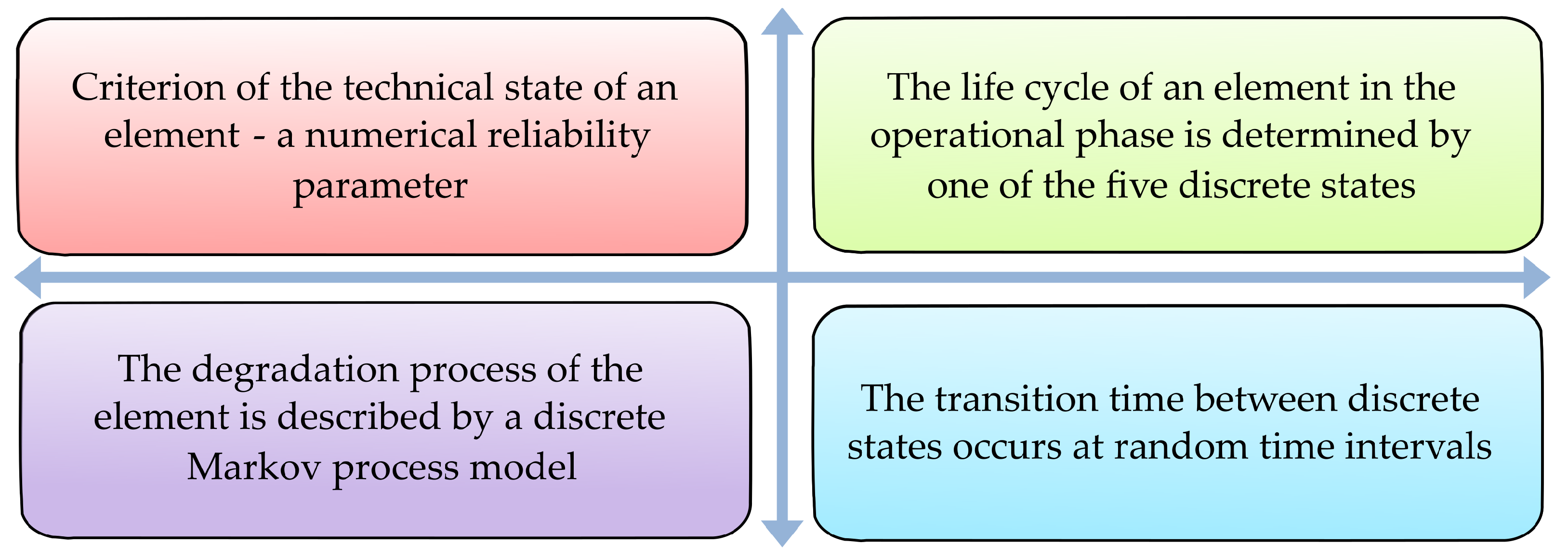
According to the requirements of the regulatory documents [16], validation calculations of load-bearing capacity are performed to determine the actual safety characteristics of the elements for refining the operational state.
The normative documents contain necessary classification tables, which are based on the assumption that widely used methods and tools are applied for inspections and examinations of bridges in the country. It should be noted that the tables in most countries are open for modernization and are constantly updated. This means that over time, experience will accumulate in inspections using advanced methods, and the tables will be supplemented with corresponding new quantitative and qualitative characteristics of operational states.
The procedure for classifying the state of bridge elements based on inspection results involves correlating defects and damages recorded during inspections with the descriptions of states provided in the degradation tables. Given that reliability (safety characteristic) is defined for each discrete state in the tables, the conclusion regarding the classification of the operational state of the element simultaneously determines its reliability.
Traditionally, three methods are used for predicting the service life of bridges: the coefficient method, the loading function method, and the principle of time segments.
The coefficient method, based on initial data, starts with a reference service life of the structure which is subsequently adjusted using coefficients. These coefficients account for factors such as the quality of construction materials, design level, manufacturing quality, internal and external environmental influences, usage of the structure, and maintenance level [22].
The loading function method is formulated as a comparison of two stochastic variables: the influence of loading and the surrounding environment, and the resistance of the structure. By comparing these two values, information about the safety and performance (reliability) of the structure over time can be obtained. In specific cases, coefficients may be expanded. For instance, material quality coefficients may vary based on material grade. This method is used for a rough assessment of the technical state using coefficients.
The next method is the time function of structure operation. Based on this function, an exponential law is used to determine the operational time of the structure and the degree of its degradation.
The proposed model for predicting the operational state is based on phenomenological classification tables of discrete states and degradation functions. This model relies on four postulates (Figure 2):
A.
The criterion for the technical state of an element is a numerical reliability parameter.
B.
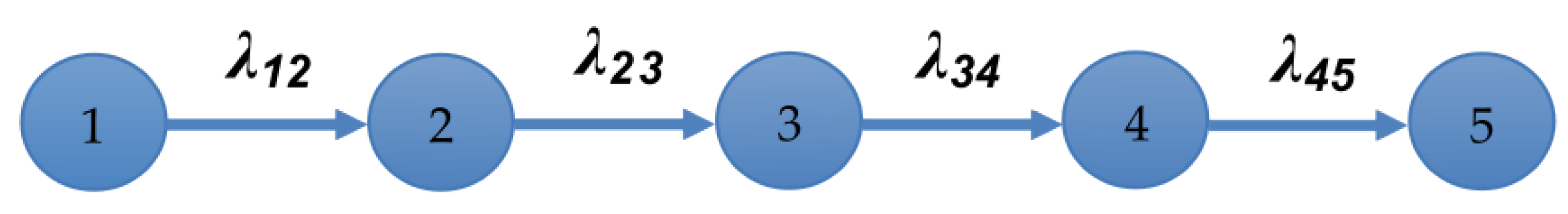
The life cycle of an element in operation is divided into 5 discrete states. Each state is described by a set of quantitative and informal (linguistic) qualitative degradation indicators, characterizing the hierarchy of element failures [23].
C.
The process of element degradation throughout the operational life cycle is described by a discrete model of a continuous-time Markov process.
D.
The time of transition between discrete states occurs at random time points.

3. Results

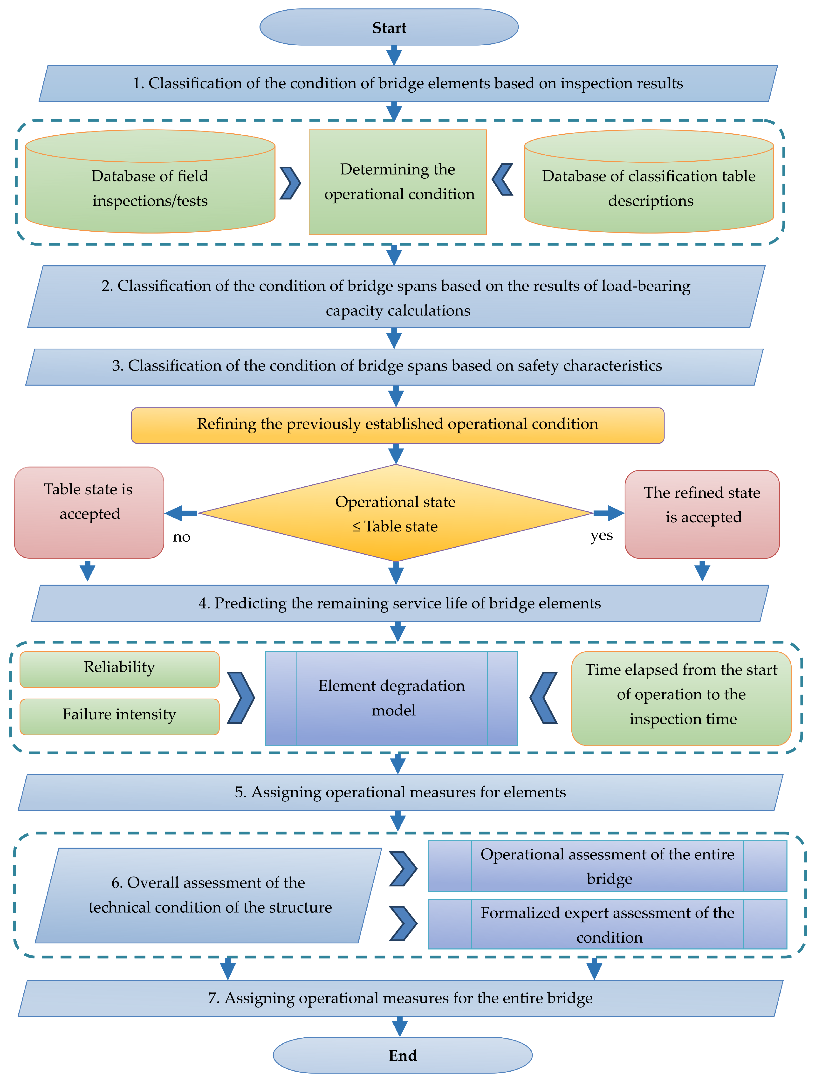
3.1. Algorithm for Assessing and Predicting the Technical Condition of the Bridge

Based on the conducted research, an algorithm for assessing and predicting the technical condition of equipment was developed (Figure 3).
The algorithm for assessing and predicting the technical condition consists of the following main steps:
Step 1: Classification of the condition of bridge elements based on inspection and/or testing results using classification tables.
The procedure for classifying the operational condition of the bridge elements based on inspection involves correlating characteristic defects, damages, and other degradation indicators recorded during inspections and tests with the description of their degradation process provided in the classification tables of the regulatory document [16]. Based on this correlation, each element is assigned to one of the five operational states (Table 1). In cases where the wear level of an element or the state of its degradation is not specified in the information tables, the expert classifies the state using the general description of the operational states of the structure. This procedure is notably subjective and heavily reliant on the expertise of the inspector conducting the survey.
Step 2: Classification of the state of bridge superstructures based on the calculation of their load-bearing capacity.
Determining load-bearing capacity is a mandatory regulatory procedure aimed at refining the classification of the operational condition of an element. Load-bearing capacity is determined with respect to temporary moving loads that were applicable at the time of design. The determination of the load-bearing capacity of superstructures is performed based on the actual dimensions of structural elements, mechanical properties of materials, and a description of observed defects recorded during inspection.
In cases where the operational condition classified by load-bearing capacity is lower than what was obtained in Step 1, this condition should be conclusively accepted.
Step 3: Classification of the state of bridge superstructures based on the results of analytical calculation of their real-time safety characteristics. This calculation serves to refine the classification of the condition.
The initial data for determining safety characteristics include inspection data with specified mechanical characteristics of materials, quantitative indicators of degradation of their cross-section, aggregated values of resistance, and loads. Parameters reflecting the probabilistic nature of stress–strain state factors of the element are coefficients of variation of strength characteristics of materials and temporary moving load. These data are independent of the current state of the bridge element and are provided in regulatory documents.
Step 4: Prediction of the remaining service life of bridge elements.
The period of trouble-free operation of the bridge is predicted in accordance with the recommendations of regulatory documents. The degradation model of the element, i.e., the transition from one operational state to another, is described as a discrete-state Markov process with continuous time. The initial data for determining the remaining service life are the reliability of the element, the time elapsed from the start of operation to the time of inspection, and the failure intensity. These data are obtained based on inspections, load-bearing capacity verification calculations, real-time safety characteristic calculations, and operational state classification.
The failure intensity for the element is found from the degradation equation as its solution under known initial conditions: the reliability of the element in the i-th operational state obtained from the classification table of operational states, and the time elapsed from the start of operation of the element to the moment of classification of its operational state. The remaining service life of the structure as a whole (prediction of the period of trouble-free operation) is estimated based on the lowest of the remaining service life indicators of the superstructures, supports, and foundations.
Step 5: Assignment of operational measures for the considered elements is carried out using normative tables. For all discrete states, the level of wear of the element (in %) and the necessary regulatory operational measures for each state are determined.
Step 6: For integral assessment of the technical condition of the structure, two indicators are introduced: operational assessment of the bridge as a whole based on basic classification and formalized expert assessment of the technical condition of the entire structure.
The operational assessment of the bridge as a whole is a comprehensive characteristic of the operational suitability of the structure in the state of its non-bearing elements. The operational condition of the bridge is classified as the lowest among the indicators of the operational condition of its three main bearing elements: superstructure, supports, and foundation.
The expert operational assessment (rating) of the bridge as a whole is an integral comprehensive characteristic of the operational suitability of the bridge, determined by the state of all seven of its elements. For this purpose, a 100-point scale of dimensionless coefficients is used.
Formalized expert assessment (rating) is used for:
  • Ranking structures within a specific road network, with the need for repair or reconstruction.
  • Planning expenditures for repairs, reconstruction, or the construction of new structures.
  • Establishing the maintenance regime of the structure.
  • Determining the timing and types of repairs.
  • Assigning parameters for strengthening and widening of the roadway.
  • Making decisions regarding the necessity and feasibility of replacement, reconstruction, or major repairs.
Depending on the rating of the structure, the need for corresponding operational measures is determined.
Step 7: Assignment of operational measures for the bridge as a whole.
This final formalized stage of the procedure involves making the necessary operational decisions in accordance with the recommendations of regulatory documents.

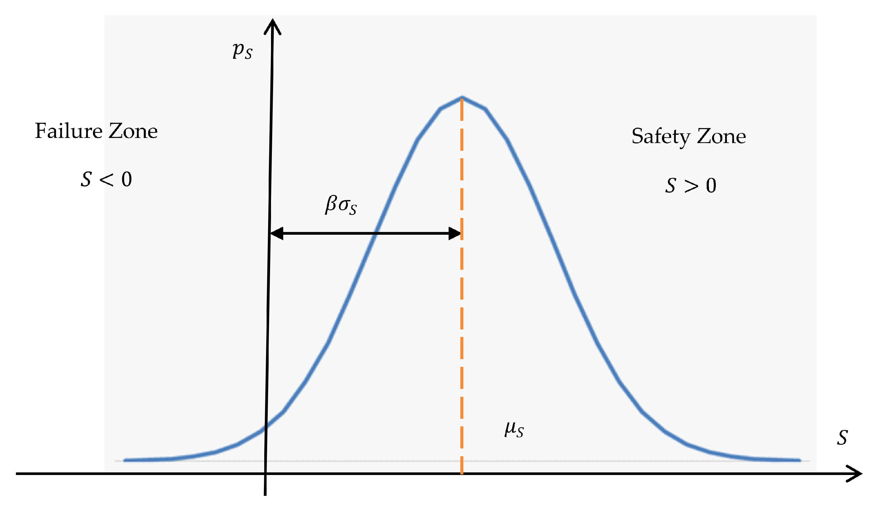
3.2. Reliability Assessment and Degradation Process Determination of Bridge Structures

In the methodology, it is assumed that reliability calculation is carried out on the theoretical basis [7,23]. In this case, the reliability of the structure (or its element) is the probability that the value of the generalized strength reserve will be positive, i.e.,
P = P r o b ( S > 0 ) ,
where P is the reliability of the structure and S is the strength reserve. The strength reserve is defined as the difference between the generalized resistance of the element and the generalized load:
S = R Q ,
where R denotes the generalized resistance of the element and Q is the generalized load on the element. In most practical tasks, the generalized resistance of the element and the load are considered random variables following a normal distribution. Therefore, according to [23,24], the strength reserve will also be a random variable, following a normal distribution (Figure 4):
μ S = μ R μ Q ; σ S = σ R 2 + σ Q 2
where μ R , μ Q denote the mathematical expectations of the generalized resistance and load, respectively, and σ R , σ Q are the standard deviations of the resistance and load distributions, respectively.
Then the probability of structural failure is determined by:
V = P r o b ( S < 0 ) = P S ( 0 ) = 0 p S d S ,
where p S is the probability function of strength reserve. Then, considering that P + V = 1 , and p S follows a normal distribution, we obtain [23]:
P = 1 2 + Φ ( β ) ,
where function ( x ) is the Gaussian probability integral. Safety characteristic β is determined by the formula
β = μ S σ S .
As seen from Figure 2, the parameter β determines the number of standard deviations within the interval from S = 0 to S = μ S . By considering (3) and (6), the safety characteristic can be expressed as
β = μ R μ Q σ R 2 + σ Q 2 .
Let us introduce a deterministic value called the factor of margin
γ = μ R μ Q .
Then, Equation (7) takes the form
β = γ 1 ν Q 2 + γ 2 ν R 2 ,
where ν R = σ R μ R and ν Q = σ Q μ Q are coefficients of variation for the variables R and Q, respectively.
The formula for determining the safety characteristic (9) has an advantage over Formula (7) because the coefficients of variation can be estimated even with insufficient statistical information regarding the structural resistance and loading.
In a separate case, when the strength of the structure can be considered a deterministic quantity ( ν R = 0 ) , Formula (9) takes the form:
β = γ 1 ν Q .
Thus, it has been shown that the reliability of the structure is uniquely expressed through the safety characteristic. It is proposed that bridge structures are divided into 5 states based on their operational condition (Table 1).
This number of states, in our view, is optimal. Each state corresponds to its own interval of β , and therefore the reliability calculated from (5). In most cases, the design value of the safety characteristic should be within the range of β = 3.8–4.5, which corresponds to the reliability interval of P = ( 0.999928 0.999997 ) . This reliability interval for bridge structures is quite sufficient. However, as experience shows, high design (or initial) reliability does not guarantee that the structure will operate without failure for the specified period required by regulatory requirements. In other words, initial reliability does not guarantee the specified service life. This is due to many factors, including the rate of material degradation, the quality of work executed, possible design flaws, and so on. Determining the time (or remaining capacity) by which the structure will transition to the 5-th (inoperative) state is the second part of the reliability theory problem.
According to the multiplication theorem, a complex event P ( t ) can be represented as the product:
P ( t ) = P 0 · P t ( t ) ,
where P 0 is the initial or design reliability at the start of structure operation ( t = 0 ) is determined by the Formula (5), P t ( t ) is the probability of failure-free operation of the structure until time t > 0 . It is assumed that when t = 0
P t ( t ) = 1 .
In other words, the function P t ( t ) can be considered as the reliability of the structure at time t > 0 , provided that its initial reliability (12) equals one.
Currently, there is no universally accepted model for determining reliability as a function of time. As one of the possible options, the research suggests determining P t ( t ) using the Markov model of damage accumulation.
The failure rate function λ f r (fail rate) is one of the most important parameters in reliability theory [23], which is associated with the reliability by the relationship:
λ f r ( t ) = 1 P d P d t .
The physical meaning of the function λ f r ( t ) is that it equals the probability of failure within the time interval ( t , t + d t ) given that the structure has been operating without failure up to time t. At the beginning of the structure’s operation, when its reliability is close to one, taking into account (4), can be expressed as:
λ f r ( t ) d P d t = d V d t .
That is why the function λ f r ( t ) is sometimes referred to as the degradation rate (reliability reduction rate) of the structure.
With the consideration of (11), the dependency (13) can be expressed as:
λ f r ( t ) = 1 P t d P t d t .
As we can see from (15), the failure intensity function does not depend on the initial reliability of the structure. If we assume that λ f r ( t ) does not depend on time ( λ f r ( t ) = λ C = c o n s t ) , then from (15) we obtain the well-known exponential degradation law:
P t ( t ) = e λ C t .
This law is widely used for solving many reliability theory problems, particularly for various functional-purpose and bridge structures.
It is worth noting that, based on practical operating experience, the failure intensity function cannot be considered constant throughout the entire life cycle. This is due to the significant role that metal and concrete corrosion plays in the degradation process of bridge structures. As of today, steel and reinforced concrete are the main materials used for bridge structures. At the beginning of a structure’s operation, when the reinforcement is covered with a protective layer of concrete, corrosion practically does not develop. Therefore, the rate of degradation, and hence the failure intensity function, will approach zero at this stage. With the development of corrosion processes, the derivative of the failure intensity function begins to increase, reliability decreases accordingly, and thus, λ f r ( t ) increases quite quickly. Therefore, the application of the exponential degradation law (16) can lead to significant errors in determining the degradation process of the structure, which in turn will lead to errors in determining the remaining resource.
Therefore, to determine the probability of failure of a structure that would correspond more to real operating conditions, the authors propose a method based on a continuous-time discrete-state Markov model.
According to this model, the transition time from one state to another occurs at random points in time. The operational states (Table 1) that a structure may be in are adopted as the states of the Markov chain. Let us consider the process graph in the form of Figure 5, where λ i j is the density of the flow of random events (transition intensity) that transfers the system from state i to state j.
In the general case, transitions between states can be arbitrary. For example, if a transition from state 3 to state 1 is possible (due to repairs), the corresponding parameter λ i j 0 applies.
It is important to emphasize that despite similar notations, the quantities λ i j and λ f r ( t ) are different functions with different physical meanings.
As known [23], a continuous-time Markov process is described by the Kolmogorov differential equations system, which in the considered case will have the form:
d p 1 d t = λ 12 p 1 ; d p 2 d t = λ 23 p 2 + λ 12 p 1 ; d p 3 d t = λ 34 p 3 + λ 23 p 2 ; d p 4 d t = λ 45 p 4 + λ 34 p 3 ; d p 5 d t = λ 45 p 4 .
In matrix form, this system takes the following form:
d p d t = A p ,
where p = [ p 1 , p 2 , p 3 , p 4 , p 5 ] T is a column vector, p i ( t ) is the probability of the system being in the i-th state, and A is the flow density matrix. For the given system (17) matrix A is of the form:
A = λ 12 0 0 0 0 λ 12 λ 23 0 0 0 0 λ 23 λ 34 0 0 0 0 λ 34 λ 45 0 0 0 0 λ 45 0 .
Since the system can only be in one of the five states, we can express it as:
i = 1 5 p i ( t ) = 1 .
Condition (20) is the normalization condition for (17).
The initial conditions for integrating (17) characterize the state of the system at time t = 0 :
p 1 ( 0 ) = 1 , p 2 ( 0 ) = p 3 ( 0 ) = p 4 ( 0 ) = p 5 ( 0 ) = 0 .
If we consider the coefficients λ i j to be independent of time, then (17) represents a system of ordinary differential equations of the first order with constant coefficients.
The solution to the system (17) for the case of a homogeneous Markov process with equal coefficients λ i j = λ = c o n s t can be obtained using the method of undetermined coefficients [23].
We can write the characteristic equation of the system (17) as:
det A k E = 0 ,
where E is a 5-th order identity matrix and k is the characteristic number.
Taking into account (19), the characteristic Equation (22) takes the form:
k ( k + λ ) 4 = 0 .
The roots of Equation (23) are the numbers k = 0 with multiplicity 1 and k = λ with multiplicity 4. Therefore, the vector of fundamental solutions q = [ q 1 , q 2 , q 3 , q 4 , q 5 ] T will have the form:
q = [ 1 , e λ t , t e λ t , t 2 e λ t , t 3 e λ t ] T .
According to the method of undetermined coefficients, we seek the solution of the system (17) in the form:
p j ( t ) = i = 1 5 C i j q i ,
where C i j the constants (undetermined coefficients) are determined from the initial conditions (21).
Thus, the solution of the system (17) takes the form:
p 1 ( t ) = e λ t , p 2 ( t ) = λ t e λ t , p 3 ( t ) = λ 2 t 2 2 e λ t , p 4 ( t ) = λ 3 t 3 6 e λ t , p 5 ( t ) = 1 1 + λ t + λ 2 t 2 2 + λ 3 t 3 6 e λ t .
It is easy to verify that the functions (26) are the solution of the system (17), which satisfy initial conditions (21), and normalization conditions (20).
The fifth state is a final state (the structure is in a non-operational state), so the probability of the structure being in a given state will be the sought reliability.
P t ( t ) = 1 p 5 ( t ) = 1 + λ t + λ 2 t 2 2 + λ 3 t 3 6 e λ t .
Taking into account (27), the failure intensity function (13) can be expressed as:
λ f r = λ 4 t 3 6 + 6 λ t + 3 λ 2 t 2 + λ 3 t 3 .
Thus, the developed methodology allows for determining the technical condition of individual bridge elements, followed by a general assessment of the entire structure as a whole.

4. Discussion

Let us conduct a numerical experiment to determine the probability function of the bridge being in the 5-th state for failure intensities of λ = 0.02 1 y e a r and λ = 0.0128 1 y e a r (Figure 6a,b).
As we can see from the provided graphs, the reliability of the structure remains practically constant in the initial stage of its operation (10–15 years). After the initial stage, depending on the value of λ ( λ = 0.02 1 y e a r and λ = 0.0128 1 y e a r ), degradation processes start to develop much faster.
Given the known initial reliability of the structure, the analytical relationship (27) allows us to determine the remaining service life, i.e., the time of operation of the structure before it transitions to the 5-th (non-operational) state. In this critical state, the reliability of the structure will be P c r = P ( t ) = 0.958351 (see Table 1).
To determine the remaining service life of the structure, the initial (design) reliability value, as practical experience shows, is very close to one. Therefore, we will consider that Equation (11) can be replaced with an approximate equality:
P ( t ) P t ( t ) .
Note that this constraint is not significant and does not alter the calculation algorithm.
To determine the remaining service life, it is convenient to express relationship (27) as a function of the parameter:
α = λ t .
Then, considering (29), we can write:
P ( α ) = ( 1 + α + α 2 2 + α 3 6 ) e α .
The graph of the function (31) is presented in Figure 7, where the horizontal lines P = c o n s t represent the reliability of the structure corresponding to its state according to Table 1.
The point of intersection of the line P c r = P ( t ) = 0.958351 with the curve (31) determines the maximum or critical value of the parameter α c r . Taking into account the condition that the design service life of the bridge is set at 100 years, from Equation (17), the failure rate λ can be obtained. Therefore, if λ = 0.0128, the structure will achieve the reliability P c r after 100 years of operation. The actual service life of individual critical elements of the bridge may be around 60–65 years. For such structures, the failure rate λ will be 0.02. Therefore, for calculations, the values λ = 0.02 and λ = 0.0128 were chosen. Then, with the known intensity value λ , we can determine the service life of the structure T as:
T = α cr λ .
From the provided graph, we determine that α c r = 1.28 . If the design service life of the bridge is T = 100 years, then from Equation (32), we obtain the intensity value λ = λ 0 = 0.0128 . This intensity corresponds to a service life of 100 years and can be referred to as the design intensity of transitions between states that the structure may be in. In reality, the value of λ can be both greater and smaller than λ 0 .
To determine the value of λ , it is necessary at a certain stage of the bridge’s operation t = t e to conduct an inspection, as a result of which the corresponding reliability of the structure P e will be determined. Based on the inspection results, the safety characteristic β e that the structure has at the moment t = t e is determined.
Using the value of reliability P e , obtained either from the graph (Figure 7) or by using appropriate programs for finding roots of functions (31), we determine the parameter α e and the intensity value λ , which is equal to:
λ = α e t e .
Thus, the remaining service life of the structure, taking into account (32) and (33), will be equal to:
Δ T = T t e = α c r α e 1 t e .
If, as a result of the inspection, only the operational state of the structure is determined, then P e is chosen from among the average reliability values for that particular state. This, of course, reduces the accuracy of forecasting the remaining service life, but can be used with insufficient information during the inspection of the structure.
It is important to emphasize that since the parameter λ characterizes the degradation process, the inspection time for its accurate determination should be no less than 10–15 years. The practical implementation of the proposed method is planned for future research.

5. Conclusions

One of the key parameters in bridge management systems is the remaining service life of the structure, which represents the predicted period of its trouble-free operation. The behavior of a bridge depends on many factors, most of which have a random nature. Therefore, it is logical that degradation models of bridges in most countries are stochastic. One such model is the Markov model of damage accumulation. A significant advantage of the Markov model is that the future behavior of the structure depends only on its present state (known as the memory less property). This enables the prediction of the remaining service life based on the results of the inspection at the current moment in time.
In many European Union countries, a discrete-time Markov model is applied, assuming that transitions from one state to another can only occur at discrete points in time. In Ukraine, a continuous-time Markov model is currently used. According to this model, transitions between states can occur at arbitrary, random points in time. The corresponding system of differential Equations (Kolmogorov equations) was derived based on the Markov model with discrete states and continuous time. The analytical solution of the system of equations using the method of undetermined coefficients allowed for the formalization of the reliability function of the structure and the failure intensity function. As a result, a reliability graph was constructed, providing a straightforward algorithm for determining the remaining service life of the structure based on the conducted inspection of the bridge’s condition.
From the provided reliability and failure intensity function graphs, it can be concluded that for a certain period (approximately 10–15 years), the reliability of the structure remains practically unchanged. This indicates that during this time, degradation processes in the structure hardly occur, if disregarding unexpected events. Therefore, the parameter λ , which characterizes the deterioration of the structure’s condition, and the corresponding remaining service life can be accurately determined only after 15 years of operation. An advantage of such a model is that the reliability function of the system can be obtained in analytical form, greatly simplifying the algorithm for determining the remaining service life.

Author Contributions

Conceptualization, K.M., A.K., V.T. and A.S.; methodology, K.M. and Y.Y.; validation, A.S. and A.B.; formal analysis, K.M. and Y.Y.; investigation, K.M., A.K., A.S., V.T. and A.B.; resources, K.M. and V.T.; data curation, K.M., A.K., A.S., V.T. and A.B.; writing—original draft preparation, K.M., A.K. and V.T.; writing—review and editing, A.S. and A.B.; visualization, A.K. and V.T.; supervision, K.M. and A.K.; project administration, A.S.; funding acquisition, A.S. and A.B. All authors have read and agreed to the published version of the manuscript.

Funding

Funded by the EU Next Generation EU through the Recovery and Resilience Plan for Slovakia under the project No. 09I03-03-V01-00104. Co-funded by the VEGA Grant Agency of the Slovak Republic, grant No. 1/0230/22.

Institutional Review Board Statement

Not applicable.

Data Availability Statement

No new data were created or analyzed in this study. Data sharing is not applicable to this article.

Conflicts of Interest

The authors declare no conflicts of interest.

References

  1. Folić, R.; Partov, D. Comparative analysis of some bridge management systems. Građev. Mater. Konstr. 2020, 63, 21–35. [Google Scholar] [CrossRef]
  2. Santamaria, M.; Fernandes, J.; Matos, J.C. Overview on performance predictive models—Application to Bridge Management Systems. In Proceedings of the IABSE Symposium 2019 Guimaraes, Guimaräes, Portugal, 27–29 March 2019. [Google Scholar]
  3. Sánchez-Silva, M.; Klutke, G.-A. Reliability and Life-Cycle Analysis of Deteriorating Systems; Springer: Cham, Switzerland, 2016. [Google Scholar]
  4. Koteš, P.; Strieška, M.; Bahleda, F.; Bujňáková, P. Prediction of RC bridge member resistance decreasing in time under various conditions in Slovakia. Materials 2020, 13, 1125. [Google Scholar] [CrossRef]
  5. Fabianowski, D.; Jakiel, P.; Stemplewski, S. Development of artificial neural network for condition assessment of bridges based on hybrid decision making method—Feasibility study. Expert Syst. Appl. 2021, 168, 114271. [Google Scholar]
  6. Mohammadzadeh, S.; Vahabi, E. Time-dependent reliability analysis of B70 pre-stressed concrete sleeper subject to deterioration. Eng. Fail. Anal. 2011, 18, 421–432. [Google Scholar] [CrossRef]
  7. Hatami, A.; Morcous, G. Reliability and Life-Cycle Analysis of Deteriorating Systems; Nebraska Transportation Center: Lincoln, NE, USA, 2011. [Google Scholar]
  8. Zayed, T.M.; Chang, L.-M.; Fricker, J.D. Statewide performance function for steel bridge protection systems. J. Perform. Constr. Facil. 2002, 16, 46–54. [Google Scholar] [CrossRef]
  9. Biondini, F.; Frangopol, D.M. Life-cycle performance of deteriorating structural systems under uncertainty. J. Struct. Eng. 2016, 16, F4016001. [Google Scholar]
  10. Rogulj, K.; KilićPamuković, J.; Jajac, N. Knowledge-based fuzzy expert system to the condition assessment of historic road bridges. Appl. Sci. 2021, 11, 1021. [Google Scholar] [CrossRef]
  11. Liang, Z.; Parlikad, A.K. A Condition-Based Maintenance Model for Assets with Accelerated Deterioration due to Fault Propagation. IEEE Trans. Reliab. 2015, 64, 972–982. [Google Scholar] [CrossRef]
  12. Eryilmaz, S. Mean Residual and Mean Past Lifetime of Multi-State Systems with Identical Components. IEEE Trans. Reliab. 2010, 59, 79–87. [Google Scholar] [CrossRef]
  13. Lantukh-Lyashchenko, A.I. Estimation of the reliability of the structure according to the Markov random process model with discrete states. Automob. Roads Road Constr. 1999, 59, 644–649. (In Ukraine) [Google Scholar]
  14. Bashkevych, I.V.; Yevseychyk, Y.B.; Medvediev, K.V.; Yanchuk, L.L. Determining the failure intensity function based on the Markov process. Automob. Roads Road Constr. 2021, 109, 79–87. (In Ukraine) [Google Scholar] [CrossRef]
  15. Bashkevych, I.V.; Yevseichyk, Y.B.; Medvediev, K.V.; Fal, A.E.; Yanchuk, L.L. Analytical model expert assessment condition of bridges. Automob. Roads Road Constr. 2022, 112, 154–162. [Google Scholar]
  16. DSTU 9181:2022; Guidelines for the Assessment and Prediction of the Technical Condition of Highway Bridges. Ministry of Regional Development of Ukraine: Kyiv, Ukraine, 2022. (In Ukraine)
  17. Slovak Road Administration. Available online: https://www.ssc.sk/en/activities/road-network-development/bridge-management/extract-of-technological-regulations-for-bridge-management.ssc (accessed on 20 September 2023).
  18. ISO 15686-1; International Organization for Standardization 2000, Building and Constructed Assets—Service Life Planning—Part 1: General Principles. ISO: Geneva, Switzerland, 2011.
  19. Hovde, P.J. The factor method for service life prediction from theoretical evaluation to practical implementation. In Proceedings of the 9th International Conference on Durability of Building Materials and Components, Brisbane, QLD, Australia, 17–20 March 2002. Paper 232. [Google Scholar]
  20. Lounis, Z.; Mirza, M.S. Reliability-based service life prediction of deteriorating concrete structures. In Proceedings of the 3rd International Conference on Concrete under Severe Conditions of Environment and Loading (CONSEC’01), Vancouver, BC, Canada, 18–20 June 2001; Volume 1, pp. 965–972. [Google Scholar]
  21. Kleiner, Y. Scheduling inspection and renewal of large infrastructure assets. J. Infrastruct. Syst. 2001, 7, 136–143. [Google Scholar] [CrossRef]
  22. Kanin, A.; Kharchenko, A.; Tsybulskyi, V.; Sokolova, N.; Shpyh, A. Construction of a simulation model for substantiating the parameters of long-term road maintenance contracts. East.-Eur. J. Enterp. Technol. 2022, 2, 33–42. [Google Scholar]
  23. Strakhova, N.Y.E.; Holubyev, V.O.; Koval’ov, P.M.; Todirika, V.V.; Khodun, V.M. Operation and Reconstruction of Bridges; Transport Academy of Ukraine: Kyiv, Ukraine, 2000. (In Ukraine) [Google Scholar]
  24. Lu, C.; Wei, Z.; Qiao, H.; Hakuzweyezu, T.; Qiao, G.; Li, K.; Zhu, B. Multi-damage accelerated life test based on the Birnbaum-Saunders reliability evaluation model. J. Asian Archit. Build. Eng. 2023, 22, 226–239. [Google Scholar] [CrossRef]
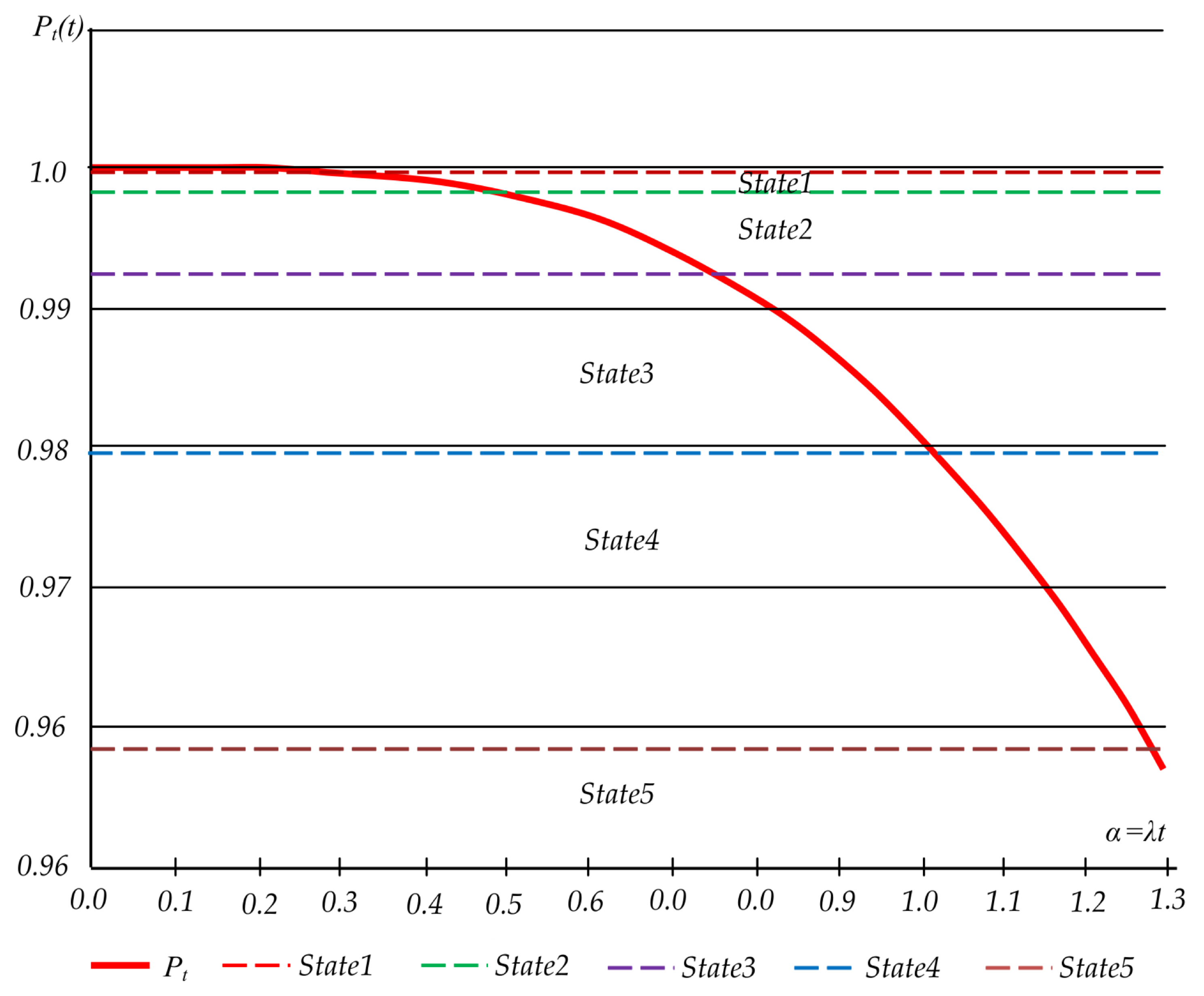
Figure 1. Conceptual model and research motivation.
Infrastructures 09 00016 g001
Figure 2. The theoretical basis of the model for assessment and prediction of the technical state of bridge elements.
Infrastructures 09 00016 g002
Figure 3. Algorithm for assessing and predicting the technical condition of the bridge.
Infrastructures 09 00016 g003
Figure 4. Strength reserve distribution function.
Infrastructures 09 00016 g004
Figure 5. State transition graph.
Infrastructures 09 00016 g005
Figure 6. Probability functions (a) and degradation rates (b) for chosen failure intensities.
Infrastructures 09 00016 g006
Figure 7. Graph of the reliability dependence on the parameter α .
Infrastructures 09 00016 g007
Table 1. Classification of operational states of elements.
Operational StateState NameReliability (According to the First Group of Limit States), PSafety Characteristic, β
State 1Serviceable0.9998443.80
State 2Limited Serviceability0.9983632.95
State 3Operational0.9924612.43
State 4Limited Operational0.9797712.05
State 5Non-Operational0.9583511.74
Disclaimer/Publisher’s Note: The statements, opinions and data contained in all publications are solely those of the individual author(s) and contributor(s) and not of MDPI and/or the editor(s). MDPI and/or the editor(s) disclaim responsibility for any injury to people or property resulting from any ideas, methods, instructions or products referred to in the content.

