Mobile Structural Health Monitoring Based on Legged Robots

Abstract

With the advancements in information, communication, and sensing technologies, structural health monitoring (SHM) has matured into a substantial pillar of infrastructure maintenance. In particular, wireless sensor networks have gradually been incorporated into SHM, leveraging new opportunities towards reduced installation efforts and enhanced flexibility and scalability, as compared to cable-based SHM systems. However, wireless sensor nodes are installed at fixed locations and need to be employed at high density to reliably monitor large infrastructure, which may cause high installation costs. Furthermore, the limited power autonomy of wireless sensor networks, installed at fixed locations for unattended long-term operation, still represents a significant constraint when deploying stationary wireless sensor nodes for SHM. To resolve the critical constraints stemming from costly high-density deployment and limited power autonomy, a mobile structural health monitoring concept based on legged robots is proposed in the study reported in this paper. The study explores the accuracy and cost-efficiency of deploying legged robots in dense measurement setups for wireless SHM of civil infrastructure, aiming to gain insights into the advantages of mobile wireless sensor nodes in general and of legged robots in particular, in terms of obtaining rich information on the structural condition. As is shown in this paper, the legged robots, as compared to stationary wireless sensor nodes, require a smaller number of nodes to be deployed in civil infrastructure to achieve rich sensor information, entailing more cost-efficient, yet accurate, SHM. In conclusion, this study represents a first step towards autonomous robotic fleets advancing structural health monitoring.

1. Introduction

The effects of climate change, such as extreme rainfall, temperature fluctuations, sea level rise, wildfires, hurricanes, increased storm surges, and floods, will accelerate the progressive deterioration of infrastructure [1]. Global infrastructure investment needs are estimated at USD 97 trillion by 2040 [2]. If the current trend of underinvestment in economic infrastructure continues, the world will face a gap in infrastructure investments of about USD 350 billion per year [3]. Regarding the deterioration of transportation infrastructure, such as bridges, roads, and railways, it is estimated that low-income countries and middle-income countries will need to spend between 0.5% and 3.3% of their gross domestic product (GDP), or USD 157 billion to USD 1 trillion, annually on new transportation infrastructure by 2030—plus additional 1–2% of their GDP on network maintenance [4]. In industrial countries, estimates show that continued underinvestment in deteriorating infrastructure will have a cascading effect on the economy and, regarding the US, will cause a loss of USD 10 trillion in GDP over the next two decades [5]. The situation in other industrial countries is similar. In Germany, almost 700 bridges are more than 100 years old, and more than 10% of highway bridges are deficient [6], highlighting the need for timely structural maintenance, which has been increasingly relying on structural health monitoring (SHM).

Structural health monitoring has been employed for more than half a century to mitigate infrastructure deterioration and its financial implications, gaining momentum with recent advancements in information, communication, and sensing technologies [7]. While early SHM case studies have been limited to civil infrastructure of high importance or of strong academic interest, today’s SHM systems have matured into a significant pillar of infrastructure maintenance, representing a supplement to traditional structural maintenance strategies, such as non-destructive testing and visual inspections [8,9]. Through obtaining structural information extracted from structural response data collected by SHM systems, damage indicators are established that may be used for facilitating predictive maintenance and advancing life-cycle management strategies [10]. Nevertheless, traditional cable-based SHM systems are capable of yielding relatively limited (spatially coarse) structural information, due to the high costs and the laborious installations of cable-based sensors. In recent years, wireless sensor networks have gradually been incorporated into SHM [11], leveraging new opportunities towards reduced installation efforts, enhanced flexibility and scalability as well as lower installation costs, as compared to cable-based SHM systems.

Besides being easy to install, flexible, and scalable, smart wireless SHM systems are capable of embedded computing and distributed-cooperative execution of SHM tasks, which enables wireless SHM systems to autonomously detect structural anomalies and to provide structural information in real time [12]. Since the merits of wireless technologies have been apparent from the very first wireless strategies in SHM, practitioners have sought to deploy wireless SHM systems of increasing density, in an attempt to obtain spatially rich information on structural conditions and resolve a major constraint of cable-based systems [13]. However, even in wireless SHM systems, the instrumentation density is limited by aesthetic and operational constraints of monitored structures, notwithstanding the less intrusive installation of wireless sensor nodes as compared to cable-based sensors. In addition, particularly dense wireless sensor networks, in which wireless sensor nodes are installed at fixed locations and are employed at high density to reliably monitor large infrastructure, may cause high installation costs, thus nullifying the cost-effectiveness of wireless SHM systems. Furthermore, the limited power of wireless sensor networks, installed at fixed locations and for unattended long-term operation, still represents a significant constraint when deploying stationary wireless sensor nodes for SHM [14]. To enrich the SHM-derived structural information, while addressing the aesthetic and operational constraints, the costly high-density deployment and the limited power of wireless sensor nodes, mobile wireless sensor networks have been proposed for SHM [15].

In a mobile wireless sensor network, each mobile sensor node is a miniature mobile robot, equipped with smart sensors, that explores its environment and exchanges information through wireless communication. Thus, both constraints inherent to stationary wireless sensor nodes can be resolved when taking advantage of mobility: First, high spatial resolutions can be achieved by cost-efficiently deploying a small number of mobile wireless sensor nodes; second, each mobile wireless sensor node can be enabled to periodically return to a base station for automatic recharging, eliminating the constraint of limited power. In the last decades, prototype mobile wireless sensor nodes have been proposed based on wheeled robots [16]. It has been demonstrated that augmenting stationary sensor networks with mobile nodes solves many design challenges that exist in stationary sensor networks. The technological foundations required to implement wheeled mobile wireless sensor nodes have been well-established, including routing protocols, architecture and topology, self-organization, energy utilization, scalability, localization, security, and privacy [17,18]. Mobile wireless sensor nodes have successfully been employed for wireless inspections and wireless structural health monitoring [19]. However, although wheeled robots deployed for mobile SHM eradicate major disadvantages of stationary wireless sensor nodes regarding high (and costly) deployment density and power consumption, wheeled robots still offer room for improvement regarding maneuverability, transversability, and efficiency. These improvements are inherent to legged robots. Since the emergence of bionics in the middle of the 20th century, legged robots, mimicking the behavior of living beings, have been an objective in robotics research, gaining new impetus with the advent of the Internet of Things and Industry 4.0 [20].

The development of legged robot locomotion has continuously been evolving over the past decades, as it offers distinct advantages compared to wheeled robots in maneuverability, transversability, and efficiency [21]. As compared to wheeled robots, legged robots have a greater ability to move on almost all surfaces in different terrains, providing better adaptability to unstructured and unknown environments. Representing a particularly promising type of legged robots, quadruped robots are ideal in terms of stability and efficiency and are thus used in applications that require high safety or high payload [22]. Being easy to control, design, and maintain, quadruped robots exhibit better equilibrium than robots with fewer legs, while walking control is not as complex as walking control of multi-legged robots [23]. Engineering tasks executed by quadruped robots include mine inspection, space exploration, or firefighting [21]. However, the utilization of quadruped robots in wireless SHM has received little attention.

This paper reports on a study proposing a mobile structural health monitoring concept based on legged, i.e., quadruped, robots, aiming to gain insights into realizing the advantages of mobile wireless sensor nodes in general and of quadruped robots in particular. The mobile SHM concept builds around an SHM methodology towards obtaining spatially rich structural information in a cost-efficient manner and at an accuracy comparable to wireless SHM with stationary wireless sensor nodes. In particular, the SHM methodology enables the piece-wise synthesis of spatially dense mode shapes, extracted by deploying the legged robots at overlapping pairs of locations on the structure. The legged robots are equipped (i) with sensors to collect acceleration data relevant to SHM of civil infrastructure, (ii) with “light detection and ranging” (Lidar) sensors for navigation, and (iii) with embedded algorithms facilitating autonomous data analysis, communication, and navigation. As will be shown in this paper, the legged robots, as compared to stationary wireless sensor nodes, require a smaller number of nodes to be deployed to achieve rich sensor information, entailing more cost-efficient SHM. As compared to wheeled robots, quadruped robots provide better maneuverability, as critical parts of civil infrastructure may be hard to reach by wheeled robots. The mobile SHM concept, with emphasis on the performance of the quadruped robots regarding the accuracy of SHM, is validated through laboratory tests and field tests, by comparing the SHM results obtained by the legged robots to the SHM results obtained by benchmark SHM systems, composed of high-precision sensors for the laboratory tests and of state-of-the-art stationary wireless sensor nodes for the field tests.

The remainder of the paper starts with a description of the SHM methodology for the mobile SHM concept, followed by the implementation of the concept into a prototype mobile SHM system based on the legged robots, placing emphasis on the modular software architecture. Then, the laboratory tests are presented, followed by the field tests conducted at a pedestrian bridge located in Hamburg, Germany. Next, the results of the laboratory and field tests are shown and compared with the benchmark SHM systems, showcasing the rich sensor information obtained by the mobile SHM system. Finally, the results are discussed, particularly focusing on the accuracy and cost-efficiency of the mobile SHM system. The paper concludes with a summary of the key findings and a discussion on future research that may be conducted to further advance this work.

2. A Mobile Structural Health Monitoring System Based on Legged Robots

In recent decades, structural analysis almost exclusively has been relying on the finite element method. Furthermore, the ability of finite element analysis to predict elaborate structural conditions in a piece-wise fashion has enabled design engineers to deviate from simple geometries and to venture into complex structural systems, which, in turn, deviate from classical structural conditions that have driven structural design for several years based on engineering intuition. However, from the perspective of structural maintenance via SHM, structural complexity inevitably raises the need for rich information on the structural condition, which cannot be retrieved with the relatively sparse SHM systems employed in current practice. The mobile SHM concept, presented in this paper, aims at enriching the information on the structural condition, while minimizing the efforts, costs, and intrusiveness, caused by dense wireless SHM systems. Specifically, the legged robots, being capable of scanning structures in detail, enable SHM practitioners to assess the condition of the structures at a structural element level and make informed decisions on the overall structural conditions. Moreover, information on a structural element level enables comparisons with elaborate finite element models, typically created as part of SHM strategies, as well as model updating.

Despite the benefits of employing legged robots for SHM, special attention should be paid to the cost efficiency of the mobile SHM concept. One of the major aspects of wireless technologies that has been appealing to practitioners is the low cost of wireless SHM systems, as compared to cable-based SHM systems, especially as far as unit prices of wireless sensor nodes are concerned. By contrast, the unit price of legged robots may be considerable. Therefore, due allowance must be made to the size of the mobile SHM system, in terms of the number of legged robots employed. In this direction, given that standard SHM data analysis methods are usually built on correlations between data sets recorded at different locations, the number of legged robots employed in this paper is reduced to the minimum, i.e., two-legged robots. For example, employing two-legged robots is in line with operational modal analysis (OMA) requirements, in which the legged robots collaboratively record and exchange SHM data to estimate mode shapes. As such, the legged robots also possess capabilities of wirelessly communicating with each other and exchanging SHM data. The following discussion centers around the SHM methodology, as well as the hardware and software implementation of the proposed mobile SHM concept.

2.1. Methodology

The methodology followed for the mobile SHM concept in this paper draws primarily from vibration-based SHM, typically conducted using acceleration response data. Although the methodology may, in theory, extend to any types of sensors attached to the legged robots, vibration-based SHM is selected, because accelerometers require neither to be fixed with strong—quasi-permanent—adhesives for measuring accurately, as is the case with strain gauges, nor to be insulated, as is the case with temperature sensors. As a result, accelerometers offer unique advantages as regards the ability of the legged robots to quickly and efficiently switch from recording acceleration response data to navigating to the next measurement location.

Following common SHM practices, information on the structural condition via vibration-based SHM is extracted through analysis of acceleration response data. Over the years, several algorithms for data analysis in vibration-based SHM have been developed, as evidenced by the large body of literature [24]. Broadly speaking, algorithms have been devised for analyzing acceleration response data to extract information in the time domain and in the frequency domain [25]. The information is usually represented in the modal domain, i.e., via estimates of mode shapes, referred to as “experimental mode shapes”. In this paper, the objective of the SHM methodology is to derive experimental mode shapes via frequency domain decomposition (FDD) [26]. In what follows, the steps of the SHM methodology are illuminated.

2.1.1. Definition of Measurement Locations

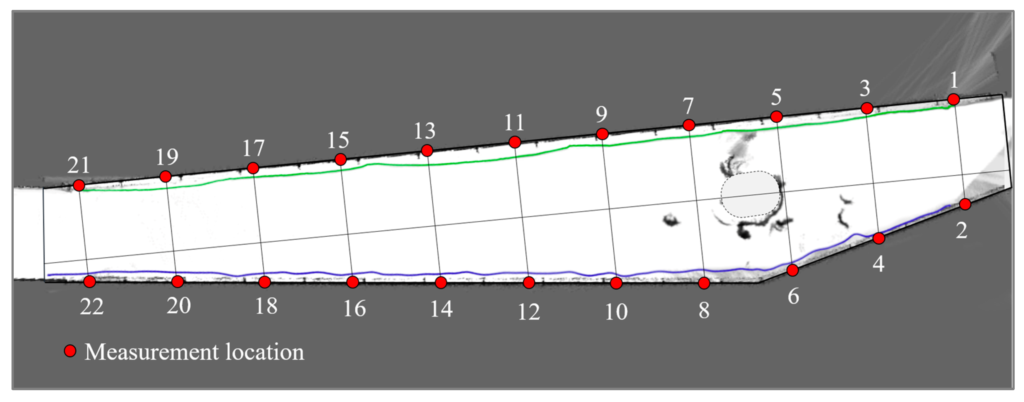
The first step of the SHM methodology involves defining the grid of measurement locations, hereinafter referred to as the “measurement grid”, on which the legged robots are tasked to record acceleration response data. Traditionally, selecting the measurement locations falls within the broad scope of “design of experiments”, which from the perspective of SHM, builds upon engineering intuition usually gained from preliminary numerical simulations. However, the mobility granted by the legged robots alleviates the SHM methodology followed in this paper from the computational burden of conducting numerical simulations for selecting the most suitable measurement locations. Specifically, representing an advantage of the legged robots, the number of measurement locations is not restricted by the finite number of stationary wireless sensor nodes, as in traditional wireless SHM systems. Therefore, defining the measurement grid follows a discretization process, similar to the discretization applied in finite element modeling, by setting a grid size, accounting for the complexity of the structure and the autonomy of the legged robots, as shown in Figure 1. Furthermore, the capability to define relatively fine discretizations allows the detection of high-order modes—provided the excitation energy in the respective frequencies is sufficiently high—that are usually topologically hard to describe with few stationary wireless sensor nodes.

The measurement grid is scanned by the two-legged robots in successive pairs of overlapping measurement locations. In other words, assuming that the measurement grid includes m locations (L = [L₁, L₂,…, L_m]^T), at least m − 1 measurement setups are conducted, ensuring that each measurement setup has one measurement location included in the previous measurement setup. As will be shown below, the overlap is necessary for computing the relative differences in amplitudes among the measurement locations, which are needed for synthesizing the experimental mode shapes.

2.1.2. Data Acquisition and Frequency–Domain Analysis

Upon reaching the jth measurement setup (pair of measurement locations in the measurement grid) (0 < j < m − 1), the legged robots start recording acceleration response data. The measurement duration, as well as the sampling frequency (f_s), are case-specifically defined by the users a priori and must be kept relatively modest to ensure that the power autonomy of the legged robots suffices to cover the entire size of the measurement grid. Care should be taken, however, that the sampling frequency is large enough to cover the frequency spectrum captured by the acceleration response data, limited by the Nyquist frequency (f_s/2), so as to ensure that the significant mode shapes are properly detected. Once the data acquisition is completed, each legged robot converts its acceleration response data into the frequency domain using the fast Fourier transform (FFT), which builds upon the discrete Fourier transform, shown below:

$${\left(Y_k\right)}_{jr}=\frac{1}{N}{\left({\displaystyle \sum _{n=0}^{N-1}{y}_n{e}^{-i2\pi k\frac{n}{N}}}\right)}_{jr}k\in \mathbb{Z}, i=\sqrt{-1}, r=1,2 0\le j\le m-1$$

(1)

In Equation (1), Y_k is the kth frequency component (k = 0 … N − 1), corresponding to a frequency equal to f_k = k·f_s/N, N is the total number of measurements for the measurement setup, y_n is the nth measurement in the acceleration response data, and i is the imaginary number. Next, each legged robot performs “peak-picking”, i.e., detection of the highest values (“resonance peaks”) among the amplitudes A_k of the Fourier values Y_k, computed according to Equation (2), that constitute candidates of modal frequency components.

$${\left(A_k\right)}_{jr}={\left(\sqrt{{\left[\Re \left(Y_k\right)\right]}^2+{\left[\Im \left(Y_k\right)\right]}^2}\right)}_{jr}$$

(2)

In Equation (2), $\mathfrak{R}$(●) and $\mathfrak{I}$(●), indicate the real part and imaginary part, respectively, of a complex number. Peak-picking in traditional SHM strategies involves visualizing the Fourier amplitude spectrum, which would require sending all the Fourier values to a centralized server, thus burdening the legged robots with extensive, power-consuming wireless communication. By contrast, peak-picking in the proposed mobile SHM concept is achieved heuristically by each legged robot in an automated manner, as described below and in the flowchart in Figure 2:

• The mean amplitude Ā is computed and used to define the threshold for peak detection. Due to noise and inaccuracies inherent to the measurements and to the Fourier transform, the non-resonance-peak amplitudes are typically non-zero. Therefore, given that the number of resonance peaks is low in typical SHM strategies, the mean amplitude provides an estimate of Fourier amplitudes attributed to noise and inaccuracies;
• The threshold for peak detection is defined as A_o = Ā + σ(A_k), where σ(●) represents the standard deviation. The standard deviation portion is added to ensure that isolated amplitudes that marginally exceed the mean amplitude are excluded from being interpreted as resonance peaks;
• The resonance peaks with the highest amplitudes (i.e., crossing the peak detection threshold) are successively detected. To confirm that the same resonance peaks are detected, the legged robots exchange information on the peaks. Upon detecting a resonance peak, the corresponding frequency and Fourier value are stored in an array and the amplitude is removed from the Fourier amplitude spectrum before proceeding with detecting the next resonance peak. Moreover, due to spectral leakage, it is expected that resonance peaks may be hardly discernible from adjacent frequency components with similar amplitudes. As a result, upon detecting resonance peak k_p, a relatively short range 2a of frequency components around the resonance peak (k_p-a, k_p+a) is also removed before proceeding with detecting the next resonance peak, to avoid duplicate peak detection of practically the same resonance peak. Nevertheless, when defining the value for 2a, care should be taken that closely spaced resonance peaks may still be detected, as shown in Figure 3. In this regard, it is generally recommended to start with a low value for 2a and dynamically modify the value, in case the resonance peaks are well-separated;
• Peak detection is terminated once all amplitudes are below the peak detection threshold.

2.1.3. Synthesis of Experimental Mode Shapes

Once the entire measurement grid has been covered, the legged robots wirelessly transmit the frequencies and Fourier values of the resonance peaks to a centralized server. Thereupon, mode shapes are extracted by applying the FDD method. The FDD method builds upon the relationship between the spectral density matrix G_x of the loads, exerted on a structure being monitored, and the spectral density matrix G_y of the acceleration response data, as expressed by the respective frequency response functions. The m × m matrix G_yk (with m representing the size of the measurement grid) at the kth frequency component is computed as follows:

$$G_{yk}=\left[\begin{array}{cccc}{S}_{11,k}& S_{12,k}& \cdots & S_{1m,k}\\ S_{21,k}& S_{22,k}& \cdots & S_{2m,k}\\ ⋮& ⋮& \ddots & ⋮\\ S_{m1,k}& S_{m2,k}& \cdots & S_{mm,k}\end{array}\right], \mathrm{with} S_{vw,k}=Y_{v,k}\cdot {\overline{Y}}_{w,k},v,w\in \left[\begin{array}{ccc}1& \dots & m\end{array}\right]$$

(3)

where S_vw,k denotes the cross-spectral density value between location v and location w at the kth frequency component of the Fourier spectrum, and the overbar indicates the complex conjugate. According to the FDD method, the singular value decomposition of G_yk is related to the experimental mode shapes, provided that the loads can be reasonably approximated as Gaussian white noise:

$$G_{yk}=U\Sigma V^{\ast }\to U=\left[\begin{array}{ccc}{u}_1& \dots & u_m\end{array}\right],u_1\propto {\phi }_k$$

(4)

In Equation (4), U and V are the matrices composed of the singular vectors, and Σ is the diagonal matrix that holds the singular values. The asterisk (*) denotes complex conjugate and transpose. Assuming that the kth frequency component is a modal component, the left-most vector of matrix U is proportional to the respective mode shape φ_k.

The direct derivation of experimental mode shapes using Equation (4) is only possible if measurements from all locations on the measurement grid are simultaneously recorded. Since in the proposed mobile SHM concept the measurement locations are covered in pairs, Equation (4) is applied for each measurement setup. In particular, for measurement setup j and at the kth (modal) frequency component, Equation (4) yields the experimental mode shape sub-vector φ_k,j, which is a 2 × 1 vector that corresponds to measurement locations v and w. Similarly, from measurement setup j + 1, the mode shape sub-vector φ_k,j+1 is obtained, including elements for measurement locations w and s. The two sub-vectors are normalized with respect to the element in the sub-vectors that represents the overlapping location w between measurement setups j and j + 1, as shown below

$$U_j=\left[\begin{array}{ccc}{u}_{1,j}& \dots & u_{m,j}\end{array}\right], u_{1,j}\propto {\phi }_{k,j} =\left[\begin{array}{cc}{\phi }_{kv,j}& {\phi }_{kw,j}\end{array}\right]$$

(5)

$$U_{j+1}=\left[\begin{array}{ccc}{u}_{1,j+1}& \dots & u_{m,j+1}\end{array}\right], u_{1,j+1}\propto {\phi }_{k,j+1} =\left[\begin{array}{cc}{\phi }_{kw,j+1}& {\phi }_{ks,j+1}\end{array}\right]$$

(6)

$${\phi }_{ks}={\phi }_{ks,j+1}\cdot \frac{{\phi }_{kw,j}}{{\phi }_{kw,j+1}},{\phi }_{kv}={\phi }_{kv,j},{\phi }_{kw}={\phi }_{kw,j}\cdot \frac{1}{{\phi }_{kw,j+1}}$$

(7)

Through the successive normalization of the sub-vectors, the full m × 1 vector of the mode shape is eventually synthesized, as exemplarily illustrated in Figure 4. Due to the successive normalization, the accuracy of the sub-vector φ_k,j+1 depends on the accuracy of the sub-vector φ_k,j. In this context, special attention must be paid that the elements in sub-vectors from successive measurement setups are of the same order of magnitude. For example, resonance peaks that in specific measurement setups have low amplitudes, such as at “zero-crossing points” of mode shapes, may result in poor normalization that may affect the accuracy of the mode shape. To avoid normalization problems in the proposed mobile SHM concept, the legged robots are granted the ability to slightly modify the topology of measurement locations at zero-crossing points of mode shapes, in case amplitudes at peaks that have been identified as resonance peaks in other measurement locations are lower than the peak detection threshold.

The mobile SHM concept is implemented into a prototype mobile SHM system. The hardware and software specifications of the mobile SHM system are illuminated in the next subsection.

2.2. Hardware Design and Implementation

The legged robots employed for the prototype mobile SHM system are of type “intelligent documentation gadgets” (IDOGs). In terms of hardware, the IDOGs are based on the robot model A1 of Unitree Robotics [27], supplemented by further hardware components required for SHM. To fulfill the tasks of the mobile SHM concept mentioned previously, the IDOGs feature capabilities of locomotion in multiple directions, localizing themselves in relation to the structure, recording acceleration response data, and processing and analyzing data on board.

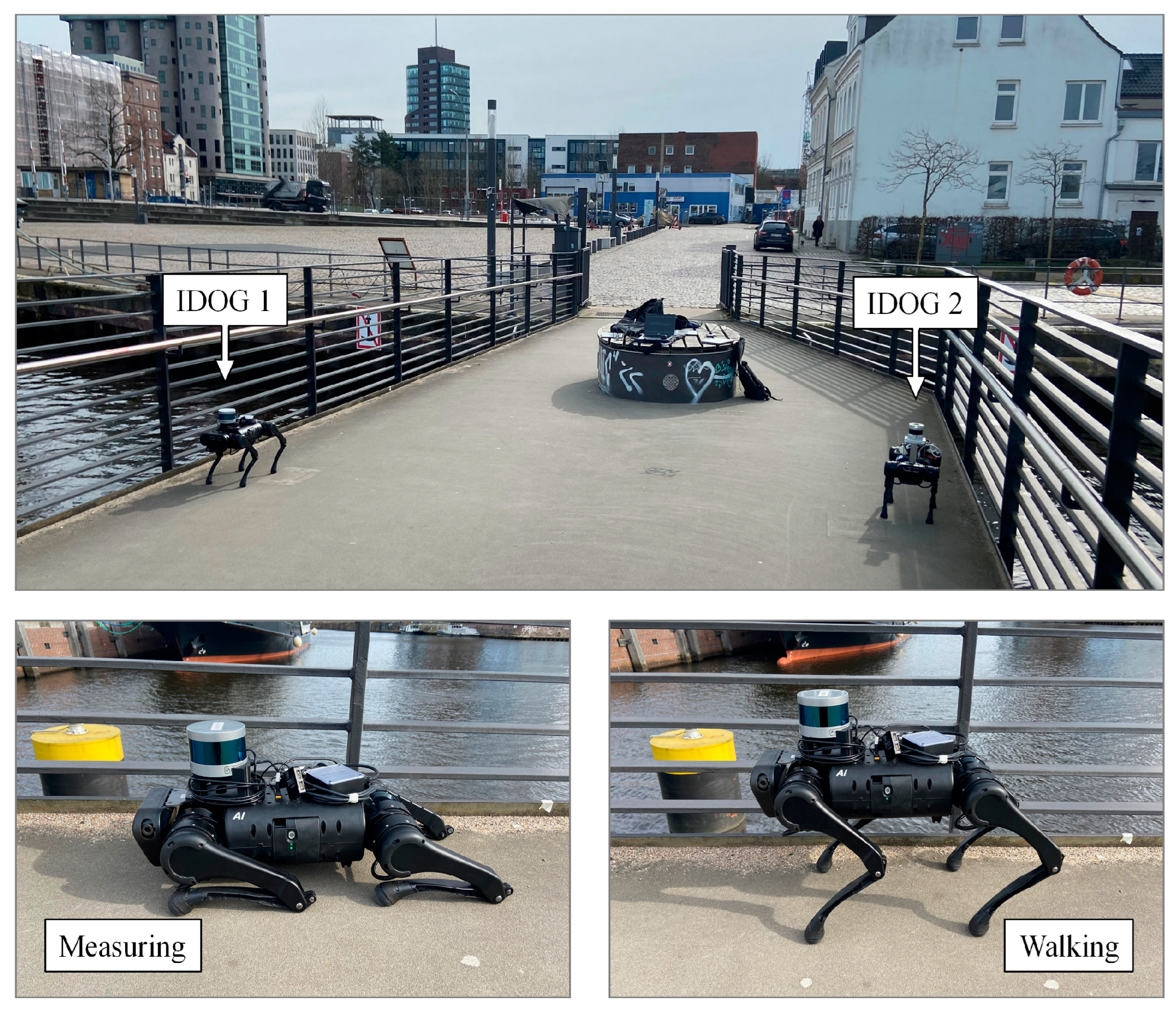
Figure 5 illustrates the hardware components. Locomotion is managed by the locomotion component, which encompasses twelve motors, distributed evenly on the four legs of the robot for granting motion at three points of each leg, namely “hip”, “knee”, and “thigh”. The enhanced locomotion achieved with the twelve motors, essentially twelve degrees of freedom, represents an important aspect of the mobile SHM system, allowing the IDOGs to easily switch from “walking posture”, which refers to simply navigating the measurement grid, to “measuring posture”, which involves lying down to record acceleration response data.

The processing component handles the computations necessary for controlling the locomotion, via the locomotion board. Moreover, the computing board, located also in the processing component, manages the processing and analysis of acceleration response data recorded by the sensors installed in the IDOGs, which reside in the sensing component.

The sensing component includes sensors that enable the IDOGs to perform the SHM tasks. In particular, to gain environmental awareness, a Lidar sensor is installed, which records point clouds (i.e., discrete sets of data points representing the exterior surfaces of nearby objects). By matching successive point clouds as the IDOGs move, the processing component creates a map of the environment and each IDOG localizes itself according to the map. The localization ensures that the IDOGs record acceleration response data at locations corresponding to the measurement grid. Connectivity between the Lidar sensor and the IDOG computing board is granted through Ethernet, which provides a bandwidth sufficient for the transmission of information to the surrounding environment. In addition, a LORD MicroStrain 3DM-GX5-25 inertial measurement unit (IMU, [28]) is attached to the sensing component for recording acceleration response data and for aiding in mapping and localization through sensor fusion. The IMU features a built-in accelerometer, a gyroscope, and a magnetometer. A USB 2.0 interface provides a connection between the IMU and the processing component. While only accelerations are of interest for SHM tasks, the combination of all three sensor types provides inertial odometry information for mapping and localization. The gyroscope measures inclinations, while the magnetometer measures magnetic field strength. The accelerometer is capable of recording acceleration response data at a maximum sampling frequency of 1 kHz, within a range of ±8 g, and with a resolution of 0.02 mg [28]. For SHM purposes, it is important that acceleration response data is recorded as closely to the surface of the structure as possible, with minimal interference from the encasements of sensing units, e.g., the mechanical components of the IDOGs. In the proposed mobile SHM system, the proximity of the accelerometers to the surface is ensured by the measuring posture, in which the IDOGs lie down on the surface, as will be demonstrated in the validation tests. The data analysis is performed onboard the IDOGs via embedded software, which is specifically designed for the mobile SHM system and involves operational modal analysis. The details of the embedded software are provided in the following subsection.

2.3. Software Design and Implementation

The embedded software for the mobile SHM system is designed on the basis of the “robot operating system” (ROS) [29], which is integrated into the IDOG processing component. ROS is an open-source middleware that provides libraries and tools for building and managing robotic software. At its core, ROS is designed modularly around a peer-to-peer network of processes that communicate in a “publish-subscribe” pattern. In particular, the basic communication implementations in ROS are called “nodes”, “messages”, and “topics”. Nodes represent processes performing computations and are able to communicate with each other by exchanging messages via topics. Messages are strictly typed data structures. Topics are “buses” over which nodes exchange messages by publishing (i.e., sending messages) and by subscribing (i.e., receiving messages).

An extract of the software, designed for the mobile SHM system and embedded into the IDOGs, is shown in Figure 6 to illustrate the general concept. With the exception of the taskScheduler and timeSynchronization components, all parts of the embedded software are based on the ROS middleware. The taskScheduler component ensures the concurrent beginning of recording acceleration response data by the IDOGs. The timeSynchronization component synchronizes the internal clocks of the IDOGs involved in the mobile SHM system, based on the “precision time protocol” defined by the IEEE 1588-2008 standard [30]. The microstrain_inertial node, which handles the operation of the IMU, publishes raw acceleration response data to the /imu/data topic. Upon completing the measurements, the embedded SHM analysis is started. First, the fft node, which subscribes to the /imu/data topic, converts the acceleration response data from the time domain into the frequency domain, via the FFT, and publishes the results to the /transform topic. The peak_picking node, in turn, subscribes to the /transform topic, detects the resonance peaks, and publishes the peaks to the /peaks topic. At the same time, the record node subscribes to and stores the raw and analyzed acceleration response data. When the required number of measurements has been recorded, the IDOGs stop recording.

For deriving the experimental mode shapes, the acceleration response data are linked with location information. The IDOGs localize themselves using Lidar-generated point clouds derived from the IMUs, based on which the IDOGs reach the target locations, defined on the measurement grid. Localization is performed in two phases. First, following up on previous work reported in [31], a “simultaneous localization and mapping” (SLAM) algorithm is employed for creating a 2D grid map of the structure. Second, after storing and linking the 2D grid map to the coordinate system in which the measurement grid is defined, the IDOGs perform “pure” localization on the map, i.e., without modifying the map. As a result of the localization, current IDOG locations are matched with the measurement grid, thus verifying that current locations match the measurement locations. In this paper, the Google Cartographer is used for both map creation and pure localization [32]. The cartographer node subscribes to the /scan topic, which provides 2D representations derived from the point clouds published by the lidar node. In addition to the point cloud data, the cartographer node takes the 2D grid map, created by the SLAM algorithm, as input and computes the position of the IDOG published in the /map topic. Furthermore, the localization serves as a basis for autonomous navigation of the IDOGs to the measurement locations. It should be noted that, in this study, to enable efficient validation of the mobile SHM system, navigation is achieved by prescribing the measurement locations a priori.

The succession of tasks towards fulfilling the SHM objectives is shown in a flowchart in Figure 7. The mobile SHM begins with time synchronization of the internal clocks of both IDOGs using the precision time protocol. Next, the sensing components are started, and both IDOGs enter a loop checking whether a measurement setup has been completed. If acceleration response data has not been recorded from the entire measurement grid, the IDOGs assume the walking posture and move to the next measurement locations, as prescribed by the respective measurement setup. The IDOGs assume the measuring posture when the measurement locations are reached. Acceleration response data acquisition begins as soon as both IDOGs have reached the designated measurement locations and have assumed the measuring postures. Then, acceleration response data is recorded for a predefined duration, and the IDOGs analyze the respective acceleration response data by computing the FFT and performing peak picking. Upon covering the entire measurement grid, the Fourier values at the peaks are sent to a centralized server, where the experimental mode shapes are synthesized, as described previously.

3. Validation of the Mobile SHM System

The mobile SHM concept proposed in this study is validated via laboratory tests and field tests, conducted with the prototype mobile SHM system. The purpose of the laboratory tests is to validate the accuracy of the IDOGs under controlled loading conditions, while the field tests are conducted to demonstrate that the mobile SHM system is capable of obtaining and analyzing rich sensor information under real-world conditions. For establishing a benchmark for comparison, benchmark SHM systems are used alongside the mobile SHM system, both in the laboratory tests and in the field tests. In what follows, the validation tests are presented and discussed.

3.1. Laboratory Tests

The laboratory tests are devised to verify the accuracy of the acceleration response data recorded by the IDOGs under controlled excitations. In the remainder of this subsection, the experimental setup used for the laboratory tests is described and the tests are presented.

The experimental setup includes a shake table, capable of inducing sinusoidal vertical motion at variable frequencies, as shown in Figure 8. The shake table superstructure comprises a 1 m × 1 m medium-density fiber plate, which is fixed to an aluminum beam and on which one IDOG is placed. The beam rests on two hydraulic cylinders, one of which is vertical and the other inclined so that the cylinders are spaced 700 mm apart at the connection points with the beam and 840 mm apart at the bases. The vertical cylinder is 2000 mm long, and the vertical distance between the base of the inclined cylinder and the base of the vertical cylinder is 290 mm. Both the beam-to-cylinder connections and the cylinder supports are pinned. The geometrical configuration of the shake table ensures that the motion of the cylinders induces a sine-wave motion to the plate.

The scenarios devised for the laboratory tests include forced vibrations at frequencies within a range from 0.5 Hz to 3.0 Hz, at steps of 0.5 Hz, as shown in

Table 1. Scenarios for the laboratory tests.

Scenario	Excitation Frequency (fo) (Hz)
1	0.5
2	1.0
3	1.5
4	2.0
5	2.5

. The displacement amplitude for all forced vibrations is 1 mm. The benchmark system, installed at the side of the IDOG, comprises a high-precision digital-output accelerometer of the type “PCB Digiducer” [33]. The sampling frequency of both the IDOG and the benchmark system is set to f_s = 25 Hz. The sampling duration for each scenario is 60 s, corresponding to N = 1500 measurements per scenario. The accuracy of the acceleration response data recorded by both the IDOG and the benchmark system is estimated through comparisons with the input acceleration amplitudes ü_o of the forced vibrations. Specifically, since the forced vibrations are harmonic sinusoidal, the input acceleration amplitude for scenario j with frequency f_j is computed as follows:

$$\left|{\ddot{u}}_{o,j}\right|=R_j\cdot {\omega }_j^2=R_j\cdot {\left(2\pi f_j\right)}^2$$

(8)

where R_j = 1 mm is the displacement amplitude and ω_j is the angular frequency. Since the FFT is defined across the total number of measurements and the highest detectable frequency is limited by the Nyquist theorem to f_s/2, the Fourier amplitude spectra Y_o,j of the IDOG and Ỹ_o,j, of the benchmark system, respectively, are “mirrored” around f_s/2. As a result, in the spectra Y_o,j and Ỹ_o,j, the input acceleration amplitude is expected to be depicted as “halved” between the first resonant peak at frequency f_p, which is the closest to the excitation frequency, and its mirror peak around f_s/2 at frequency f_fs–p. Therefore, the metrics for comparison are (i) the root mean squared error ε_o between the Fourier amplitudes Y_o,j of the IDOG and ü_o,j/2 and (ii) the root mean squared error ε₁ between the Fourier amplitudes Ỹ_o,j, of the benchmark system and ü_o,j/2, for all b = 6 scenarios, as shown in Equation (9).

$${\epsilon }_o=\frac{1}{b}{\displaystyle \sum _{j=1}^b{\left(\raisebox{1ex}{${\ddot{u}}_{o,j}$}\!\left/ \!\raisebox{-1ex}{$2$}\right.-Y_{o,j}\right)}^2}{\epsilon }_1=\frac{1}{b}{\displaystyle \sum _{j=1}^b{\left(\raisebox{1ex}{${\ddot{u}}_{o,j}$}\!\left/ \!\raisebox{-1ex}{$2$}\right.-{\tilde{Y}}_{o,j}\right)}^2}$$

(9)

3.2. Field Tests on a Real-World Pedestrian Bridge

To demonstrate that the mobile SHM system is capable of obtaining and analyzing rich sensor information under real-world conditions, field tests are conducted on a pedestrian bridge. In this subsection, the bridge and the experimental setup for the field tests are presented, followed by a description of the field tests.

3.2.1. Description of the Pedestrian Bridge and the Benchmark SHM System

The field tests were conducted on the “Citadel Bridge”, located in Hamburg, Germany. The bridge, illustrated in Figure 9, facilitates pedestrian traffic over the Lotse Canal, and it was completed in 2016. The structural system of the bridge comprises two segments, one “fixed” segment and one “revolving” segment (Figure 10), which allows naval traffic along the canal. The fixed segment, which has a length of 12.5 m and a constant width of 3.25 m, rests at its south end on a reinforced concrete pier (“Pier 1”) and abuts, at its north end, the Lotse square (“Lotseplatz”) quay wall. The revolving segment has a length of 33 m and variable width between 3.25 m and 5.65 m. At the location with the largest width, the revolving segment rests on a reinforced concrete pier (“Pier 2”), which is equipped with rotary actuators that enable the rotation of the segment about the vertical axis. When the bridge is open to pedestrian traffic, the revolving segment rests at its north end on Pier 1, next to the fixed segment, via hydraulic supports, and abuts, at its south end, the “Kanal square” quay wall. The decks of both segments of the bridge consist of steel trapezoidal box sections of variable heights with transversal stiffeners.

The benchmark system used for the field tests consists of wireless sensor nodes of type Microstrain G-Link-200 [34]. Each wireless sensor node of the benchmark system features a triaxial micro-electro-mechanical-systems accelerometer, measuring at a selectable range of up to ±8 g at sampling frequencies up to 4096 Hz. Moreover, since the experimental setup of the prototype mobile SHM system includes, as previously illuminated, two IDOGs, the benchmark system also encompasses two wireless sensor nodes, installed alongside the IDOGs in each measurement setup. To ensure synchronization between the benchmark system and the IDOGs, the precision time protocol, introduced above, is again invoked. The synchronization between the IDOGs and the benchmark system is verified via post-processing, i.e., upon completing the acquisition of acceleration response data, based on a synchronization approach presented in previous work [35].

3.2.2. Field Tests on the Bridge

Since the two segments of the pedestrian bridge are statically independent of each other, each segment exhibits distinct structural dynamic behavior. The field tests in this study focus on the revolving segment, which is more flexible than the fixed segment and, thus, more likely to undergo unfavorable vibrations. Following up on the steps of the methodology previously presented, the first step of the validation tests is to define the measurement grid on the revolving segment. Representing a trade-off between the power autonomy of the IDOGs and the spatial density of the experimental mode shapes to be extracted, a measurement grid with 3.0 m spacing is defined, as shown in Figure 11.

As can be seen from Figure 11, the number of measurement locations is smaller than the total number of grid points. The reasoning behind designating specific points on the measurement grid as measurement locations and neglecting the inner grid line stems from the nature of experimental mode shapes. Specifically, since the deck deformations are expected to be small under the effect of relatively low loads, considered in operational modal analysis, the cross-section of the deck is expected to remain straight with negligible shear deformations. As a result, capturing the structural response (via acceleration response data) only at the edges of the deck is sufficient to describe both the vertical translational and the torsional components of the experimental mode shapes, since deformations in the transversal direction relative to the edges are negligible.

The 22 measurement locations of the measurement grid are covered in pairs with overlapping locations, thus forming 21 measurement setups, as shown in

Table 2. Measurement setups.

Setup	Location of IDOG 1	Location of IDOG 2	Setup	Location of IDOG 1	Location of IDOG 2
1	1	2	12	11	14
2	1	4	13	13	14
3	3	4	14	13	16
4	3	6	15	15	16
5	5	6	16	15	18
6	5	8	17	17	18
7	7	8	18	17	20
8	7	10	19	19	20
9	9	10	20	19	22
10	9	12	21	21	22
11	11	12

. The field tests start with the IDOGs navigating to the measurement locations of the first setup, as shown in Figure 12 (top). Upon reaching the locations, the IDOGs assume the measuring posture, which ensures adequate attachment of the accelerometer to the surface of the deck (Figure 12, bottom left). One sensor node of the benchmark system is placed next to each IDOG The IDOGs synchronize the internal clocks and record acceleration response data for a duration of 60 s at a sampling frequency of 100 Hz. Next, the acceleration response data is analyzed via the embedded FFT algorithm of the IDOGs, and the resonance peaks are detected. IDOG 1 sends the frequencies of the resonance peaks to IDOG 2, which verifies that the resonance peaks detected by both IDOGs correspond to the same frequencies. Resonance peaks with low amplitudes that are detected only by one IDOG are eventually considered spurious and are discarded. Then, the IDOGs assume the walking posture and navigate to the measurement locations of the next setup (Figure 12, bottom right). The process is repeated until all 21 measurement setups have been covered. Upon completing all measurement setups, the IDOGs send the Fourier values at the resonant peaks to a centralized server, where the experimental mode shapes are synthesized.

3.3. Results and Discussion

The outcomes of the validation tests are presented and discussed in this subsection. First, the results of both the laboratory tests and the field tests are presented, in terms of resonance peaks and mode shapes. Next, the quality of the acceleration response data, collected by the mobile SHM system, is verified against acceleration response data collected by the benchmark system. Finally, the localization results are illuminated.

3.3.1. Results

The results of the laboratory tests are summarized in

Table 3. Results of the laboratory tests.

Scenario	Excitation Frequency (Hz)	Frequency at First Peak fk (Hz)		Amplitude at First Peak Ak (m/s2)		üo/2	εo	ε1
		IDOG	Benchmark	IDOG	Benchmark
1	0.5	0.488	0.488	0.004	0.003	0.005	0.0088	0.0085
2	1.0	1.025	0.977	0.013	0.011	0.020
3	1.5	1.514	1.514	0.035	0.030	0.044
4	2.0	2.002	2.002	0.079	0.079	0.079
5	2.5	2.490	2.490	0.105	0.119	0.123
6	3.0	3.027	3.027	0.175	0.190	0.178

. In particular, the frequency and amplitude of the first peak, which corresponds to the excitation frequency, are presented both for the IDOG and for the benchmark system, along with the input acceleration amplitude ü_o/2 and the root mean squared errors ε_o and ε₁.

As can be seen from Table 3, the root mean squared error of the IDOG is relatively close to the root mean squared error of the benchmark system with the high-precision accelerometer. Therefore, the IDOG is capable of accurately capturing acceleration response data under forced vibrations. Furthermore, the amplitudes of the IDOG are in relatively close proximity to the input acceleration amplitudes, with small discrepancies being attributed to FFT-related factors, such as spectral leakage, which, as evidenced by the amplitudes of the benchmark system, are hard to eradicate even with high-precision accelerometers.

In

Table 4. Peak-picking results of the field tests (IDOGs).

Setup	IDOG 1				IDOG 2
	f1 (Hz)	f2 (Hz)	f3 (Hz)	f4 (Hz)	f1 (Hz)	f2 (Hz)	f3 (Hz)	f4 (Hz)
1	3.08	4.36	-	-	3.08	4.36	-	-
2	3.05	4.31	-	-	3.05	4.31	-	-
3	3.06	4.35	-	-	3.06	4.35	-	-
4	3.06	4.31	-	-	3.06	4.31	-	-
5	3.04	4.37	-	-	3.04	4.37	-	-
6	3.06	4.33	7.41	10.52	3.06	4.33	7.41	10.52
7	3.06	4.41	7.52	10.53	3.06	4.41	7.52	10.53
8	3.05	4.33	7.28	10.56	3.05	4.33	7.28	10.56
9	3.10	4.31	7.42	10.53	3.10	4.31	7.42	10.53
10	3.03	4.32	7.17	10.52	3.03	4.32	7.17	10.52
11	3.06	4.30	7.28	10.58	3.06	4.30	7.28	10.58
12	3.04	4.32	7.42	10.60	3.04	4.32	7.42	10.60
13	3.06	4.38	7.32	10.53	3.06	4.38	7.32	10.53
14	3.08	4.31	7.21	10.57	3.08	4.31	7.21	10.57
15	3.05	4.31	7.38	10.55	3.05	4.31	7.38	10.55
16	3.06	4.32	7.41	10.52	3.06	4.32	7.41	10.52
17	3.03	4.26	7.34	10.49	3.03	4.26	7.34	10.49
18	3.05	4.28	7.39	10.60	3.05	4.28	7.39	10.60
19	3.06	4.30	7.34	10.57	3.06	4.30	7.34	10.57
20	3.06	4.31	7.36	10.51	3.06	4.31	7.36	10.51
21	3.04	4.30	7.41	10.61	3.04	4.30	7.41	10.61

, the peak-picking results of the field tests are summarized. Specifically, the frequencies of the peaks detected from each IDOG for each measurement setup are shown. For comparison purposes, the respective frequencies of the benchmark system are shown in

Table 5. Peak-picking results of the field tests (benchmark system).

Setup	Benchmark System 1				Benchmark System 2
	f1 (Hz)	f2 (Hz)	f3 (Hz)	f4 (Hz)	f1 (Hz)	f2 (Hz)	f3 (Hz)	f4 (Hz)
1	3.07	4.34	-	-	3.07	4.34	-	-
2	3.05	4.28	-	-	3.05	4.28	-	-
3	3.06	4.33	-	-	3.06	4.33	-	-
4	3.06	4.30	-	-	3.06	4.30	-	-
5	3.04	4.36	-	-	3.04	4.36	-	-
6	3.05	4.35	7.40	10.52	3.05	4.35	7.40	10.52
7	3.06	4.30	7.50	10.52	3.06	4.30	7.50	10.52
8	3.05	4.30	7.07	10.54	3.05	4.30	7.07	10.54
9	3.05	4.30	7.22	10.51	3.05	4.30	7.22	10.51
10	3.05	4.31	7.15	10.50	3.05	4.31	7.15	10.50
11	3.05	4.30	7.30	10.56	3.05	4.30	7.30	10.56
12	3.06	4.31	7.35	10.59	3.06	4.31	7.35	10.59
13	3.06	4.34	7.30	10.51	3.06	4.34	7.30	10.51
14	3.07	4.30	7.31	10.59	3.07	4.30	7.31	10.59
15	3.05	4.33	7.38	10.52	3.05	4.33	7.38	10.52
16	3.05	4.30	7.30	10.51	3.05	4.30	7.30	10.51
17	3.07	4.27	7.32	10.52	3.07	4.27	7.32	10.52
18	3.06	4.31	7.33	10.56	3.06	4.31	7.33	10.56
19	3.03	4.33	7.30	10.56	3.03	4.33	7.30	10.56
20	3.05	4.30	7.34	10.55	3.05	4.30	7.34	10.55
21	3.04	4.29	7.39	10.59	3.04	4.29	7.39	10.59

.

As can be seen from Table 4 and Table 5, the peak-picking results between the mobile SHM system and the benchmark system are close. Moreover, random variations of the resonant frequencies between successive setups follow similar trends in both SHM systems. Four resonance peaks are identified in total, with the respective frequencies being f₁ ≈ 3.1 Hz, f₂ ≈ 4.4 Hz, f₃ ≈ 7.4 Hz, and f₄ ≈ 10.6 Hz. The respective mode shapes (φ_m and φ_b of the mobile SHM system and the benchmark system, respectively) synthesized upon performing FDD in each measurement setup are illustrated in Figure 13 and tabulated in

Table 6. Mode shape vectors.

Point	Mobile SHM System				Benchmark System
	φm1	φm2	φm3	φm4	φb1	φb2	φb3	φb4
1	−1.121	1.186	-	-	−1.095	1.145	-	-
2	−1.000	1.000	-	-	−1.000	1.000	-	-
3	−0.531	0.481	-	-	−0.523	0.509	-	-
4	−0.487	0.410	-	-	−0.483	0.426	-	-
5	−0.179	0.095	-	-	−0.179	0.033	-	-
6	−0.095	0.030	-	-	−0.112	0.047	-	-
7	0.057	−0.039	−0.505	0.460	0.063	−0.032	−0.138	0.486
8	0.034	−0.039	0.372	0.647	0.040	−0.054	0.095	0.642
9	0.255	−0.209	−0.660	2.108	0.281	−0.194	−0.363	2.369
10	0.236	−0.241	0.596	2.066	0.260	−0.257	0.374	2.230
11	0.590	−0.504	−0.790	3.447	0.603	−0.469	−0.583	3.578
12	0.560	−0.491	0.817	4.040	0.554	−0.466	0.572	4.207
13	0.806	−0.776	−0.867	3.344	0.813	−0.780	−0.832	3.741
14	0.853	−0.819	0.965	2.876	0.875	−0.791	0.766	3.038
15	0.951	−0.953	−1.128	4.698	0.965	−0.937	−1.267	3.665
16	1.000	−1.000	1.000	1.000	1.000	−1.000	1.000	1.000
17	0.935	−0.962	−1.384	−9.968	0.934	−0.939	−1.576	−5.921
18	0.953	−0.954	1.372	−7.172	0.967	−0.939	1.574	−5.900
19	0.773	−0.776	−1.143	−31.461	0.745	−0.819	−1.716	−10.246
20	0.778	−0.785	1.174	−24.509	0.800	−0.784	1.754	−12.158
21	0.370	−0.381	−0.601	−28.204	0.351	−0.410	−1.160	−8.706
22	0.350	−0.335	0.600	−27.313	0.346	−0.370	1.149	−8.731

.

From Figure 13 and Table 6, it is evident that the mode shapes computed by the IDOGs are in close proximity with the mode shapes extracted with the benchmark system. The first two resonance peaks exhibit mode shapes that, between Pier 1 and Pier 2, are combinations of sinusoidal and hyperbolic sinusoidal functions, indicative of fixed-pinned beams. It can therefore be conjectured that the support on Pier 1 is simple (i.e., “pinned”), whereas the rotary mechanism on Pier 2 behaves as fixed support. Moreover, the part of the deck between Pier 2 and the Kanal square quay wall exhibits the mode shapes of a cantilever beam. Due to the fixed connection of the deck on Pier 2 and the subsequent restraint in the longitudinal displacement of the deck, it is expected that the first translational longitudinal mode shape comprises—apart from the longitudinal component—a vertical component, which is similar to the mode shape of the first translational vertical mode shape. As a result, the first two mode shapes are similar to each other. To distinguish the mode shapes, measurements in three directions would be necessary, which fall beyond the scope of this paper. The third resonance peak is characterized by torsional mode shapes that are detectable only between Pier 1 and Pier 2 in both systems. The absence of the resonance peaks in the cantilever beam may be attributed to the fixity against torsion, offered by the support of Pier 2. Finally, the fourth resonance peak corresponds to a translational mode shape with one nodal point and is also detectable only between Pier 1 and Pier 2. The lack of symmetry in the fourth mode shape is attributed to the variable cross-section of the deck, which increases in flexibility towards Pier 2, where the largest modal amplitudes are observed.

A limitation of the mobile SHM system, as a consequence of the non-permanent installation of the legged robots, is the lack of long-term acceleration response data that would help characterize the variability of the mode shapes due to diurnal/nocturnal cycles or due to seasonal effects. As has been shown in literature, resonance peaks and mode shapes may vary significantly due to the aforementioned effects [36]. It is therefore recommended, to deploy the mobile SHM system more than once at different times of day and under different climatic conditions so as to corroborate the accuracy and investigate the variability of the resonance peaks and the experimental mode shapes.

3.3.2. Data Quality Assurance

To verify the quality of the acceleration response data, collected by the mobile SHM system, the data were checked for consistency, accuracy, completeness, and integrity. Furthermore, a metric for comparison between the mode shapes of the mobile SHM system and the mode shapes of the benchmark system, the “modal assurance criterion” (MAC), was applied [37].

$${\mathrm{MAC}}_{ij}\left\{{\phi }_{mi},{\phi }_{bj}\right\}=\frac{{\left|{\phi }_{mi}^T\cdot {\phi }_{bj}\right|}^2}{\left({\phi }_{mi}^T\cdot {\phi }_{mi}\right)\cdot \left({\phi }_{bj}^T\cdot {\phi }_{bj}\right)}i,j=\mathrm{1\dots 4}$$

(10)

The MAC values are presented in the form of a matrix, shown in Figure 14. MAC values close to unity indicate large similarity between the mode shape vectors, whereas values close to zero represent low similarity. The data of Setup 12 is provided in the Supplementary Materials, Listing S1.

The similarity between the mode shapes extracted by the mobile SHM system and the mode shapes computed by the mobile SHM system, observed in the mode shape plots of Figure 13 and in the mode shape vectors in Table 6, is corroborated by the MAC values shown in Figure 14. Minor discrepancies are only observed in high-order mode shapes, which are more sensitive to external interference, e.g., from ambient noise. As a result, the quality of the acceleration response data, as well as the capability of the mobile SHM system to yield mode shapes of comparable accuracy as a wireless SHM with stationary sensor nodes, is validated in real-world conditions with a minimal deployment of two-legged robots, thus ensuring cost-effective SHM.

3.3.3. Localization Results

The localization results are visualized in Figure 15. As can be seen, the map was created using Lidar data, and Cartographer is linked to the measurement grid shown in Figure 11. The IDOGs move alongside the deck edges and collected the acceleration data in close proximity to the measurement positions defined in the measurement grid.

4. Summary and Conclusions

Structural health monitoring (SHM) has become a crucial component of infrastructure maintenance, leveraging advancements in information, communication, and sensing technologies. Cable-based SHM systems are gradually being replaced by wireless sensor networks, taking advantage of reduced installation efforts, increased flexibility, and scalability. However, wireless sensor nodes need to be deployed at high density to reliably monitor civil infrastructure, causing high costs. Moreover, stationary wireless sensor nodes have limited power autonomy, representing a significant constraint for unattended long-term operation.

To resolve the critical constraints stemming from costly high-density deployment and limited power autonomy, a mobile structural health monitoring concept based on legged robots has been proposed. The legged robots are equipped with sensors to collect acceleration data pertinent to SHM of civil infrastructure, with cameras and Lidar sensors for navigation, and with embedded algorithms that allow for data communication, processing, analysis, and synchronization. Laboratory tests and field tests, conducted on a pedestrian bridge, have been devised to validate the accuracy and cost-efficiency of the legged robots deployed in dense measurement setups for wireless SHM of civil infrastructure, aiming to gain insights into the advantages of mobile wireless sensor nodes in general and of legged robots in particular, in terms of obtaining rich information on the structural condition. Measurements recorded by the legged robots of the mobile SHM system have been compared with measurements obtained by high-precision benchmark SHM systems. The laboratory tests have showcased the capability of the mobile SHM system to collect measurements of high accuracy under controlled excitation conditions. Moreover, the field tests have demonstrated the capacity of the mobile SHM system to yield rich modal information in real-world conditions.

As has been shown in this paper, the legged robots, as compared to conventional stationary wireless sensor nodes deployed for SHM, require a smaller number of nodes to be installed in civil infrastructure to achieve rich sensor information, entailing more cost-efficient, yet accurate, SHM. In conclusion, this study represents a first step towards autonomous robotic fleets advancing structural health monitoring. Future research will focus on further advancing the perception of the robots with respect to incorporating semantic and 3-dimensional information of structures, aiming to improve autonomous navigation when performing SHM tasks.

References

1. Pudyastuti, P.; Nugraha, N.A. Climate change risks to infrastructures: A general perspective. In Proceedings of the AIP 4th International Conference on Engineering, Technology, and Industrial Application, Surakarta, Indonesia, 13–17 December 2017; Prasetyo, H., Hidayati, N., Setiawan, E., Widayatno, T., Eds.; AIP Publishing: Melville, NY, USA, 2017. [Google Scholar]
2. World Economic Forum. Infrastructure around the World Is Failing. Here’s How to Make It More Resilient. 2019. Available online: https://www.weforum.org/agenda/2019/01/infrastructure-around-the-world-failing-heres-how-to-make-it-more-resilient/ (accessed on 28 April 2023).
3. Woetzel, J.; Garemo, N.; Mischke, J.; Hjerpe, M.; Palter, R. Bridging Global Infrastructure Gaps; McKinsey Global Institute, McKinsey & Co.: New York, NY, USA, 2016. [Google Scholar]
4. Koks, E.E.; Rozenberg, J.; Zorn, C.; Tariverdi, M.; Vousdoukas, M.; Fraser, S.A.; Hall, J.W.; Hallegatte, S. A global multi-hazard risk analysis of road and railway infrastructure assets. Nat. Commun. 2019, 10, 2677. [Google Scholar] [CrossRef] [PubMed]
5. American Society of Civil Engineers. Smart Infrastructure. 2021. Available online: https://www.asce.org/topics/smart-infrastructure (accessed on 28 November 2022).
6. Delhaes, D. Bridges at risk: The Renovation Backlog Continues [Brücken in Gefahr: Der Sanierungsstau hält an]. 2021. Available online: https://www.handelsblatt.com/politik/deutschland/investitionen-bruecken-in-gefahr-der-sanierungsstau-haelt-an/27623112.html (accessed on 6 June 2022).
7. Farrar, C.R.; Worden, K. An introduction to structural health monitoring. Philos. Trans. R. Soc. A 2007, 365, 303–315. [Google Scholar] [CrossRef] [PubMed]
8. Lynch, J.P.; Loh, K.J. A summary review of wireless sensors and sensor networks for structural health monitoring. Shock Vib. 2006, 38, 91–130. [Google Scholar] [CrossRef]
9. Dragos, K.; Smarsly, K. A hybrid system identification methodology for wireless structural health monitoring systems based on dynamic substructuring. In Proceedings of the SPIE Smart Structures/NDE Conference: Sensors and Smart Structures Technologies for Civil, Mechanical, and Aerospace Systems, Las Vegas, NV, USA, 20–24 March 2016; Lynch, J.P., Ed.; SPIE: Bellingham, WA, USA, 2016. [Google Scholar]
10. Smarsly, K.; Hartmann, D.; Law, K.H. An integrated monitoring system for life-cycle management of wind turbines. Smart Struct. Syst. 2013, 12, 209–233. [Google Scholar] [CrossRef]
11. Dragos, K.; Smarsly, K. A comparative review of wireless sensor nodes for structural health monitoring. In Proceedings of the 7th International Conference on Structural Health Monitoring of Intelligent Infrastructure, Turin, Italy, 1–3 July 2015; De Stefano, A., Ed.; Curran Associates, Inc.: Red Hook, NY, USA, 2015; pp. 170–179. [Google Scholar]
12. Smarsly, K.; Lehner, K.; Hartmann, D. Structural health monitoring based on artificial intelligence techniques. In Proceedings of the ASCE International Workshop on Computing in Civil Engineering, Pittsburgh, PA, USA, 24–27 July 2007; Soibelman, L., Akinci, B., Eds.; ASCE: Reston, VA, USA, 2007; pp. 111–118. [Google Scholar]
13. Smarsly, K.; Petryna, Y. A decentralized approach towards autonomous fault detection in wireless structural health monitoring systems. In Proceedings of the 7th European Workshop on Structural Health Monitoring (EWSHM), Nantes, France, 8–11 July 2014; Volume 20. [Google Scholar]
14. Smarsly, K.; Law, K.H.; König, M. Resource-efficient wireless monitoring based on mobile agent migration. In Proceedings of the SPIE Smart Structures/NDE Conference: Health Monitoring of Structural and Biological Systems, San Diego, CA, USA, 6–10 March 2011; Kundu, T., Ed.; SPIE: Bellingham, WA, USA, 2011. [Google Scholar]
15. Zhu, D.; Yi, X.; Wang, Y.; Lee, K.-M.; Guo, J. A mobile sensing system for structural health monitoring: Design and validation. Smart Mater. Struct. 2010, 19, 55011–55021. [Google Scholar] [CrossRef]
16. Dantu, K.; Rahimi, M.; Shah, H.; Babel, S.; Dhariwal, A.; Sukhatme, G.S. Robomote: Enabling mobility in sensor networks. In Proceedings of the 4th International Symposium on Information Processing in Sensor Networks, Los Angeles, CA, USA, 15 April 2005; IEEE: Piscataway, NJ, USA, 2005; pp. 404–409. [Google Scholar]
17. Panagopoulos, A.D. Handbook of Research on Next Generation Mobile Communication Systems; IGI Global: Hershey, PA, USA, 2016. [Google Scholar]
18. Ramasamy, V. Mobile wireless sensor networks: An overview. In Wireless Sensor Networks—Insights and Innovations; Sallis, P.J., Ed.; IntechOpen Ltd.: London, UK, 2017; pp. 3–19. [Google Scholar]
19. Huston, D.R.; Esser, B.; Gaida, G.; Arms, S.; Townsend, C. Wireless inspection of structures aided by robots. In Proceedings of the SPIE 6th Annual International Symposium on NDE for Health Monitoring and Diagnostics: Health Monitoring and Management of Civil Infrastructure Systems, Newport Beach, CA, USA, 4–8 March 2001; Chase, S.B., Aktan, A.E., Eds.; SPIE: Bellingham, WA, USA, 2001; pp. 147–154. [Google Scholar]
20. Rubio, F.; Valero, F.; Llopis-Albert, C. A review of mobile robots: Concepts, methods, theoretical framework, and applications. Int. J. Adv. Robot. Syst. 2019, 16. [Google Scholar] [CrossRef]
21. Biswal, P.; Mohanty, P.K. Development of quadruped walking robots: A review. Ain Shams Eng. J. 2021, 12, 2017–2031. [Google Scholar] [CrossRef]
22. Gonçalves, R.S.; Carvalho, J.C.M. Review and latest trends in mobile robots used on power transmission lines. Int. J. Adv. Robot. Syst. 2013, 10, 1–14. [Google Scholar] [CrossRef]
23. Smarsly, K.; Worm, M.; Dragos, K.; Peralta, J.; Wenner, M.; Hahn, O. Mobile structural health monitoring using quadruped robots. In Proceedings of the SPIE Smart Structures/NDE Conference: Sensors and Smart Structures Technologies for Civil, Mechanical, and Aerospace Systems, Long Beach, CA, USA, 3 March 2022. [Google Scholar]
24. Kullaa, J. Vibration-based structural health monitoring under variable environmental or operational conditions. In New Trends in Vibration Based Structural Health Monitoring; Deraemaeker, A., Worden, K., Eds.; Springer Verlag AG: Vienna, Austria, 2010; pp. 107–181. [Google Scholar]
25. Fritzen, C.-P. Vibration-based structural health monitoring—Concepts and applications. Key Eng. Mat. 2005, 293–294, 3–20. [Google Scholar]
26. Brincker, R.; Zhang, L.; Andersen, P. Modal identification of output-only systems using frequency domain decomposition. Smart Mater. Struct. 2001, 10, 441–445. [Google Scholar] [CrossRef]
27. Unitree Robotics. A1 Robot. 2020. Available online: https://www.unitree.com/products/a1/ (accessed on 23 June 2022).
28. Microstrain Sensing. MicroStrain Sensing Product Datasheet: 3DM-GX5-AHRS; Parker Hannifin Corp: Williston, VT, USA, 2020. [Google Scholar]
29. Quigley, M.; Gerkey, B.; Conley, K.; Faust, J.; Footey, T.; Leibs, J.; Berger, E.; Wheeler, R.; Ng, A. ROS: An open-source Robot Operating System. In Proceedings of the International Conference on Robotics and Automation, Kobe, Japan, 12–17 May 2009. [Google Scholar]
30. The Institute of Electrical and Electronics Engineers. IEEE Standard for a Precision Clock Synchronization Protocol for Networked Measurement and Control Systems (1588-2008); IEEE: New York, NY, USA, 2008. [Google Scholar]
31. Smarsly, K.; Dragos, K.; Stührenberg, J.; Worm, M. Structural health monitoring of civil infrastructure using mobile robots. In Proceedings of the 19th International Conference on Computing in Civil and Building Engineering (ICCCBE), Cape Town, South Africa, 26–28 October 2022. [Google Scholar]
32. Hess, W.; Kohler, D.; Rapp, H.; Andor, D. Real-time loop closure in 2D LIDAR SLAM. In Proceedings of the International Conference on Robotics and Automation, Stockholm, Sweden, 16–21 May 2016; IEEE: Piscataway, NJ, USA, 2016; pp. 1271–1278. [Google Scholar]
33. PCB Piezotronics. Digiducer USB Digital Accelerometer 333D01 Datasheet; The Modal Shop/PCB Piezotronics: Cincinnati, OH, USA, 2021. [Google Scholar]
34. Microstrain Sensing. Microstrain Sensing Product Datasheet: G-Link-200; Parker Hannifin Corp: Williston, VT, USA, 2020. [Google Scholar]
35. Dragos, K.; Makarios, T.; Karetsou, I.; Manolis, G.D.; Smarsly, K. Detection and correction of synchronization-induced errors in operational modal analysis. Arch. Appl. Mech. 2020, 90, 1547–1567. [Google Scholar] [CrossRef]
36. Peeters, B.; De Roeck, G. One year monitoring of the Z24-Bridge: Environmental influences versus damage events. Earthq. Eng. Struct. Dyn. 2000, 30, 149–171. [Google Scholar] [CrossRef]
37. Allemang, R.J. The modal assurance criterion—Twenty years of use and abuse. J. Sound Vib. 2003, 37, 14–23. [Google Scholar]
Figure 1. Examples of measurement grids: (a) fine discretization for a complex structure and (b) coarse discretization for a simple structure.
Infrastructures 08 00136 g001
Figure 2. Flowchart for the automated peak-picking employed for the proposed mobile SHM concept.
Infrastructures 08 00136 g002
Figure 3. Examples of removing amplitudes from the Fourier spectrum following peak detection: A narrow range of 2a for closely spaced resonance peaks (left) and a wide range of 2a for well-separated resonance peaks (right).
Infrastructures 08 00136 g003
Figure 4. Exemplary synthesis of a mode shape from several measurement setups.
Infrastructures 08 00136 g004
Figure 5. Hardware components of the IDOG.
Infrastructures 08 00136 g005
Figure 6. Extract of the software embedded in the IDOGs.
Infrastructures 08 00136 g006
Figure 7. SHM tasks conducted by the embedded software designed for the IDOGs.
Infrastructures 08 00136 g007
Figure 8. Experimental setup for the laboratory tests.
Infrastructures 08 00136 g008
Figure 9. Views of Citadel Bridge, Hamburg, Germany.
Infrastructures 08 00136 g009
Figure 10. (a) View of the pedestrian bridge and (b) a depiction of piers and segments.
Infrastructures 08 00136 g010
Figure 11. Measurement grid and measurement locations.
Infrastructures 08 00136 g011
Figure 12. Simultaneous collection of acceleration response data (top), walking posture of the IDOG (bottom left), measuring posture of the IDOG (bottom right).
Infrastructures 08 00136 g012
Figure 13. Vibration mode shapes of the pedestrian bridge.
Infrastructures 08 00136 g013
Figure 14. MAC matrix comparing the mode shapes calculated by the mobile SHM system and by the benchmark system.
Infrastructures 08 00136 g014
Figure 15. 2D grid map of Citadel bridge with trajectories of IDOG 1 (top path, green) and IDOG 2 (bottom path, blue) created by Cartographer and overlaid with the measurement grid.
Infrastructures 08 00136 g015