Article

Installation and Use of a Pavement Monitoring System Based on Fibre Bragg Grating Optical Sensors

by
Francisco J. P. Rebelo
1,
Joel R. M. Oliveira
1,*,
Hugo M. R. D. Silva
1,
Jorge Oliveira e Sá
2,
Vânia Marecos
3 and
João Afonso
4
1
Department of Civil Engineering, Institute for Sustainability and Innovation in Structural Engineering, University of Minho, 4800-058 Guimaraes, Portugal
2
ALGORITMI Research Centre, Department of Information Systems, University of Minho, 4800-058 Guimaraes, Portugal
3
Laboratório Nacional de Engenharia Civil, 1700-066 Lisboa, Portugal
4
Mota-Engil Group, 4300-454 Porto, Portugal
*
Author to whom correspondence should be addressed.
Infrastructures 2023, 8(10), 149; https://doi.org/10.3390/infrastructures8100149
Submission received: 30 July 2023 / Revised: 29 September 2023 / Accepted: 9 October 2023 / Published: 13 October 2023
(This article belongs to the Special Issue Sustainable and Digital Transformation of Road Infrastructures)

Abstract

:
The evolution of technological tools, namely affordable sensors for data collection, and the growing concerns about maintaining roads in adequate conditions have promoted the development of continuous pavement monitoring systems. This paper presents the installation and use of an innovative pavement monitoring system, which was developed to measure the effects of vehicle loads and temperature on the performance of a pavement structure. The sensors used are based on fibre Bragg grating optical technology, collecting data about the strains imposed in the pavement and the temperature at which those measurements are made. The site selection for the system’s installation and the essential installation details to ensure successful data collection are addressed. A calibration procedure was implemented by performing falling weight deflectometer tests and passing preweighed heavy vehicles over the sensors. In addition to validating the system installation, the results obtained in the calibration confirmed the importance of adequately choosing the distance between sensors. Differences of 50 mm in the position of the load may cause differences of about 20% to 25% in the resulting strains. These results confirmed the importance of increasing the sensor concentration in wheel paths. Furthermore, for loads between 25 kN and 65 kN, raising the temperature by 8 °C caused an increase of about 20% in the horizontal tensile strains measured in the pavement. In summary, it was possible to conclude that this innovative system is capable of capturing the effects of temperature and vehicle speed on the response of the pavement, which may be considered an advantage of this type of monitoring system when compared to those that are only used to determine the loads applied to the pavement or to characterise the type of vehicle.

1. Introduction

Roadways are essential infrastructures for the development of any country, representing a large part of the investment made in public assets. Due to the growing population and consequent goods consumption, transportation needs, especially on highways, are also increasing, demanding a higher investment in constructing and maintaining this essential infrastructure [1]. The preservation of road pavement state depends on several factors, including its design process, composition, and sound maintenance and rehabilitation policies. These policies are even more critical with the growing concern for sustainability.
During their lifecycle, many road pavements have to support loads significantly higher than those for which they were designed, which leads to faster degradation than initially expected [2]. Ai et al. [3] studied the influence of various factors such as axle configuration, axle load, speed, and temperature on different types of asphalt pavements with specific vehicles, showing that pavement strains increased with increasing temperature and axle load. Combining these effects leads to fatigue damage of the surface layers, decreasing the structure’s lifetime.
Thus, improved road monitoring techniques are necessary to ensure traffic safety and quality throughout the pavement lifecycle [4]. Some of the main road pavement distresses can be assessed through visual inspection. However, the extensive length of any road network hinders this task, making it difficult to correctly and timely determine the pavement condition. Thus, structural health monitoring techniques can be used to save human resources. One advantage of these techniques is the possibility of obtaining a real-time understanding of road conditions by collecting data on the structural integrity of the entire infrastructure and not just of its upper layers [5].
Over recent decades, various monitoring methods have been applied to road pavements, potentially analysing parameters such as strain, stress, temperature, moisture, and deflection. In 1991, Sebaaly et al. [6] applied different types of sensors (pressure cell, strain gauge, moisture sensor, and transverse vehicle location sensor) to evaluate the effect of passing trucks. In Huff et al. [7], the response given by piezoelectric sensors was studied to obtain dynamic pavement deflection data. During one year of monitoring, Bayat et al. [8] also used strain gauges and temperature sensors on a test track to measure strains induced by both the temperature and the application of different vehicle loads. Also, in the work presented by Duong et al. [8], an asphalt pavement section subjected to heavy traffic (around 4500 trucks per day) was instrumented with strain gauges, geophones and temperature probes and monitored continuously for 18 months, concluding that temperature and the degree of bonding between the various pavement layers play a significant role in the response given.
More recently, optical sensors with FBG technology have been used instead of strain gauges in different structural monitoring systems, including pavements, because they present several advantages compared to other measuring systems. Liu et al. [9] tested the dynamic strain response of different asphalt pavement structures according to the base course. The sections were instrumented with FBG sensors, and the results generated exciting conclusions, including that the loads’ position significantly influences the peak value of dynamic strain response. In the study presented by Kara De Maeijer et al. [2], focusing on heavy-duty pavements, a prototype monitoring system based on FBG sensors was installed on a CyPaTs test track and in the port of Antwerp. This system comprised a series of sensors that captured strain and temperature information between four asphalt layers to better understand how these layers respond under heavy loads. The sensors were applied prior to the laying of the asphalt layers. The results proved the potential of this solution to monitor pavement responses and demonstrated the best procedures for applying the sensors on the pavement.
Tan et al. [10] compared the results obtained with FBG sensors and strain gauges to improve the optical sensors’ calibration method. By monitoring the dynamic response in three-point bending tests on small beams, the tensile strain of the beam bottom given by the strain gauge was compared with the theoretical results and the results given by the FBG sensors. According to specific and well-defined loading conditions, it was possible to relate the peak values between the two technologies and calibrate the equation obtained for the FBG sensors.
Over the past few years, temperature compensation in FBG sensors has been extensively studied using solutions based on distributed optical fibre sensors. The studies that have been conducted prove the importance of the temperature effect on FBG sensors, highlighting the need for this process to be performed with caution using different techniques and ways of combining optical sensors [11,12,13,14]. Wang et al. [15] performed laboratory tests on samples to propose a method to improve the temperature compensation, considering the interfacial interaction between the structure and the bonded FBG according to different temperature and loading conditions. Leal-Junior et al. [16] developed an FBG sensor based on a single polymer diaphragm for measuring pressure and temperature and compared the results obtained with a transient heat conduction model. This study concluded that the root mean square error was higher in the presence of variation in both parameters, the error being 3.88 °C and 5.13 kPa for temperature and pressure, respectively.
Han et al. [17] studied the deformation compatibility between the embedded strain sensor and asphalt layer, concluding that it is the key to ensuring the precise measurement of mechanical response. However, good deformation coordination may be difficult to maintain under different environments due to the viscoelasticity of asphalt mixture. They concluded that strain sensors with stiffness moduli similar to the asphalt layers are recommended in the dynamic response monitoring of pavement structures. Similar conclusions were obtained by Liu et al. [18] in a study where FBG sensors were compared to resistive sensors through laboratory and finite element modelling processes. They also observed that FBG sensors are more appropriate to measure horizontal strains when compared to resistive sensors.
The work discussed in the present manuscript aims to present an innovative pavement monitoring system based on FBG optical sensors implemented on a highway section in Portugal. This solution allows real-time monitoring of the mechanical conditions of the structure, measuring the effects of each traffic load on the pavement near the bottom of the asphalt layer, where cracking problems usually begin. This information was unavailable through other existing monitoring solutions and is essential to improve our knowledge regarding the causes of pavement distress. The subsequent data collection and analysis will help in scheduling future maintenance procedures. Over the last few months, several steps were carried out to prepare for the installation of the monitoring system. These steps included defining the system’s architecture, selecting the type and quantities of sensors, the laboratory calibration of the sensors (by performing four-point bending and wheel tracking tests) [19], and validation of the installation procedures in a small trial section built at the National Laboratory of Civil Engineering.

2. Characteristics of Optical Sensors

2.1. Fibre Bragg Grating Sensors

In the second half of the twentieth century, the development of optical technology and its sensors revolutionised the telecommunications industry due to its enormous advantages over the dominant technologies. As time went by, and the level of knowledge of the technology increased, its application was extended to several areas, including the monitoring of structures [20].
The various characteristics of fibre-optic sensors make their use in pavement monitoring a very suitable solution. These include immunity to electromagnetic fields, high sensitivity, small size, and resistance to harsh environments when adequately protected [5,15]. Fibre Bragg grating sensors are one type of sensor based on fibre optics and are incredibly reliable [21]. The multiplexity of this technology is another feature differentiating FBG sensors because several Bragg wavelengths can be defined for numerous sensors placed in series on a single fibre-optic cable. In this situation, only the spectral band of each sensor must be respected so that the reflected signals do not cross. This feature allows a single optical fibre over tens of meters, instrumented with many sensors, which can even measure several parameters in addition to deformation (strains) and temperature, such as acceleration and pressure [16,22].
However, in addition to being expensive, the sensors and the optical fibre become fragile if not adequately protected. It is expected that these disadvantages will tend to disappear or become less relevant as technology evolves.
This type of sensor is created by exposing a portion of optical fibre a few millimetres long to a UV laser beam. The marking will change some of the optical characteristics of the fibre, with great importance for the refractive index. This change in the refractive index will cause only a portion of the incoming light to be reflected (based on the new refractive index), creating a characteristic wavelength for each sensor [23].
When the fibre-optic cable is stretched or compressed, the characteristic Bragg wavelength of the reflected light will change. This value is read by a piece of equipment called an interrogator, which recognizes the characteristic wavelength and the new characteristic Bragg wavelength. The interrogator then converts the wavelength variation into length units, and it is possible to interpret the variation in fibre length or strain.
This technology has the characteristic that only the Bragg wavelength defined within a narrow spectrum will be reflected and received by the interrogator, causing the other signals from other sensors with different wavelengths to propagate along the optical fibre with only residual variations [5].
For the sensor to function, it is essential that the marking remains intact, not disturbing the defined Bragg wavelength. Equations (1)–(4) [20,24,25] can be used to calculate the strains imposed by the external deformations and temperature variations when using FBG sensors. Equation (1) proves that the central wavelength of the reflected signal corresponds to the Bragg condition:
λ = 2 × neff × Λ,
where λ is the Bragg wavelength, neff is the effective refractive index, and Λ is the microstructure period. The parameters neff and Λ are susceptible to external disturbances such as temperature and deformation, and changes in these indicators will determine changes in the Bragg wavelength.
Equation (2) translates the strain variation due to an external deformation:
Δ λ 1 λ 1 = Δ λ ε λ 1 = ( 1 P e ) × ε ,
where Δλε is the wavelength due to the deformation, ε is the longitudinal deformation, and Pe is the effective photo-elastic constant from the fibre’s core.
Equation (3) translates the variation in wavelength due to temperature variations:
Δ λ 2 λ 2 = Δ λ T λ 2 = ( α + ξ ) × Δ T ,
where ΔλT, ΔT, α, and ξ are, respectively, the wavelength variation due to temperature, the temperature variation, the coefficient of thermal expansion, and the thermo-optic coefficient related to the change in refractive index with temperature.
Equation (4) represents the junction of the deformation and temperature effects in an FBG sensor.
Δ λ λ = Δ λ ε λ 1 + Δ λ T λ 2 = ( 1 P e ) × ε + ( α + ξ ) × Δ T .
These sensors cannot distinguish whether wavelength changes occur due to temperature or external load effects (deformations), so it is necessary to decouple both effects. Therefore, specific procedures have been created to compensate for the effect of temperature on strain measurements. Typically, an additional FBG temperature sensor is installed (only affected by temperature) in a series with FBG strain sensors, and its results are used as input for a temperature compensation algorithm.
Consequently, it is possible to particularise the deformation caused only by external loads in the FBG sensor by knowing the combined effect of load and temperature deformation in the sensor and compensating for the component corresponding only to the temperature deformation. However, calibration is essential to ensure the quality of the results obtained by these sensors.

2.2. Fibre Bragg Grating Coating and Protection

The literature review demonstrated that one of the main difficulties in using FBG sensors is ensuring the correct stress transmission between the asphalt material and the sensors. Nevertheless, many solutions to overcome this problem have been developed in the last few years.
For example, Kara De Maeijer et al. [26] tested two ways to apply FBG sensors on asphalt layers. The first consisted of implementing sensors on prefabricated asphalt samples in the base layer, and the second consisted of installing the same sensors directly on the surface of the previously mentioned asphalt layer. The survival rate of the sensors was 100%, indicating that these methodologies can be applied in monitoring heavy-duty asphalt pavements.
Xiang and Wang [27] took a different approach concerning the FBG sensor coating by developing an asphalt mastic containing an FBG sensor inside to monitor distributed strains in beams. The theoretical analysis of strain transmission was used to improve the encapsulation design and reduce measurement error. The prototype was also tested at standard temperature and traffic loads, indicating that the proposed solution obtained satisfactory laboratory and in situ results.
Zhou et al. [24] developed an FBG sensor packaged in fibre-reinforced polymer for 3D structural strain monitoring, with optimised dimensions according to the road structure. Comparisons of the actual results with the simulations proved that the developed FBG sensor provided effective and reliable information about the strain distribution on the pavement.
The approach used in the current work consisted of initially performing laboratory tests on beams and slabs with FBG sensors with different encapsulations and resins from which the sensors’ readings were calibrated. The laboratory study also defined the solution for installation on the actual pavement. Therefore, a fibreglass rod was instrumented with a series of FBG sensors and used as a support for the optic cable, and the set was then inserted in a groove cut in the pavement that was subsequently filled with an appropriate resin (QuiniResin Fix) [28] selected during the laboratory work. This approach for the post-installation of FBG sensors in road pavements, transversally to the traffic direction and embedded in a fibreglass rod (for protection), can be considered an innovative solution since no other similar application has been found in the literature, namely, in a recent review on this subject [29].

3. Methods for Developing the Pavement Monitoring System

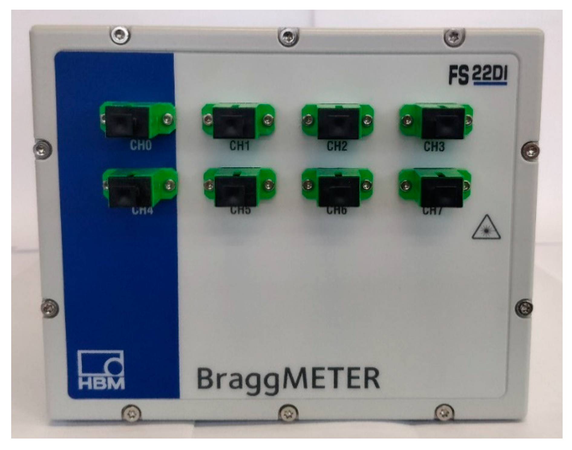
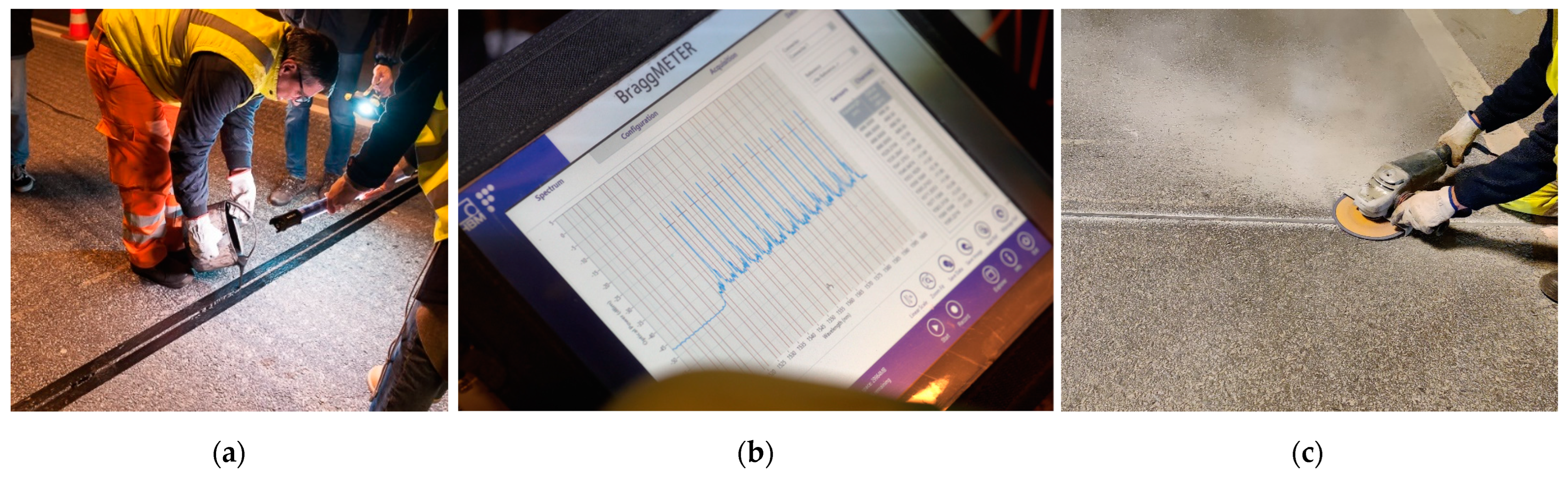
3.1. Data Acquisition System (Interrogator)

The optical interrogator is a piece of equipment essential for operating the monitoring system with FBG sensors and can perform static (e.g., temperature) or dynamic (e.g., traffic load) measurements. This optoelectronic device works as a measurement unit/data acquisition system, reading the signals reflected by the FBG sensors.
A single device can receive data from dozens of FBG sensors due to the multiplexing characteristic of the technology and the various reading channels of the device. This feature allows the same device to collect data on different parameters, even at different acquisition rates. A BraggMETER interrogator (Figure 1) was used in the present work, with a maximum acquisition rate of 1000 readings per second. Additionally, this type of FBG technology presents a very high resolution/repeatability (<1.5 pm) and stability/reproducibility (5 pm) [23].
The Catman data acquisition program is the native software used by this equipment. This tool is used to visualise and analyse the information collected by the interrogator from the various sensors. The analysis can be performed in real time or post-processing. The adaptability of the software to the needs of each situation is a critical factor for its use, as it is possible to customise it according to the objectives of each use through the creation of different graphs, tables, and other forms of visualisation. Nevertheless, other data processing and analytical tools can also be used for the same purpose [30].

3.2. Pavement Monitoring System Architecture

After defining the sensor technology to be used and identifying some of the main challenges that its installation would involve, the monitoring system’s architecture was defined, covering features such as:
  • The type of information to be collected (which determines the type of sensors to be used);
  • The location of the sensors;
  • The use of protection, coatings, or resins;
  • The application procedures;
  • The interrogator connection to the communication network infrastructure.
Given the strength and flexibility of fibreglass rods, this material was used to protect the optical sensors’ physical integrity. Thus, the rod (with a circular cross-section) was machined to create a notch where the fibre-optic cable containing the sensors would be inserted and then glued with a resin suitable for this purpose, as illustrated in Figure 2. A diameter of approximately 4 mm was chosen for the fibreglass rod. The fibre-optic cable had a diameter of approximately 125 μm.
The number of sensors each fibreglass rod would have, the respective spacing between the sensors, and the number of rods to be installed in the pavement section were defined according to the specific characteristics of the pavement of this project’s selected site. Thus, two types of rods were defined according to the number and spacing of sensors. The first type comprised fifteen strain sensors and one temperature sensor, and the second type included seven strain sensors and one temperature sensor. In order to monitor the performance of two traffic lanes and the measurement of the traffic speed, each lane was instrumented with two fibreglass rods (i.e., one of each type).
In order to increase the valuable information obtained from the monitoring system and optimise its cost, each traffic lane was instrumented with one of the rods with more sensors and another with fewer sensors. Each lane should have at least two rods to determine the speed of the passing vehicles. Furthermore, one of these rods should comprise many sensors to cover the lateral distance more efficiently and allow a better understanding of the transversal strain distribution resulting from the pavement response when subjected to vehicle loads.
The following criteria were taken into account to choose the spacing between the sensors:
  • Each traffic lane is about 3.35 m wide;
  • The width of a heavy vehicle is approximately 2.55 m;
  • The average width of one heavy vehicle tyre is about 30 cm.
In order to obtain a better characterisation of the loads and consequent strains registered in the pavement, through the analysis of the transversal strain basins, a higher density of FBG sensors was considered for the positions corresponding to the common pavement wheel path.
Figure 3 schematically shows the final architecture of each type of instrumented rod used in the pavement monitoring system.
As shown later, these fibreglass rods instrumented with FBG sensors were installed in a groove cut in the pavement. The width of the groove and the resin used to fill it were defined in previous phases of the project, both in the laboratory and in the intermediate physical model installed at the National Laboratory of Civil Engineering (LNEC) facilities. Thus, the groove in the pavement section would have a width of 1 cm, and the resin chosen to fill it was the QuiniResin Fix, which is a high-performance polymer adhesive used in various highway applications (filling of grooves, sealing of cracks, bonding of several elements) [28].

3.3. Site Selection for Pavement Monitoring System Installation

The site selected to implement the pavement monitoring system (Figure 4) is located in the country’s northeast on the IC5 highway, which belongs to the Portuguese national road network.
This site would have to meet several criteria given the stated objectives and characteristics of the monitoring system, among which the following can be highlighted:
  • Easy access and connection to an electrical power supply;
  • Access to an underground infrastructure to route the fibre-optic cables;
  • Presence of a roadside technical cabinet nearby to install the interrogator;
  • Access to a communication network in the technical cabinet to transfer the data collected in the interrogator to an external database.
An additional advantage of the selected site is being relatively close to an assistance and maintenance road administration centre, allowing easy and quick access to the equipment should any operation be necessary.
The location where the monitoring system was installed has a three-lane carriageway, two lanes in the uphill gradient direction and one in the downhill gradient direction. The monitoring system was installed in the two uphill lanes to compare the strains measured in a fast (left) and a slow (right) traffic lane, as shown in Figure 5.
Considering that heavy vehicles generally circulate in the slow lane, the monitoring system would be used to compare the effects of different loads and speeds on pavement performance.

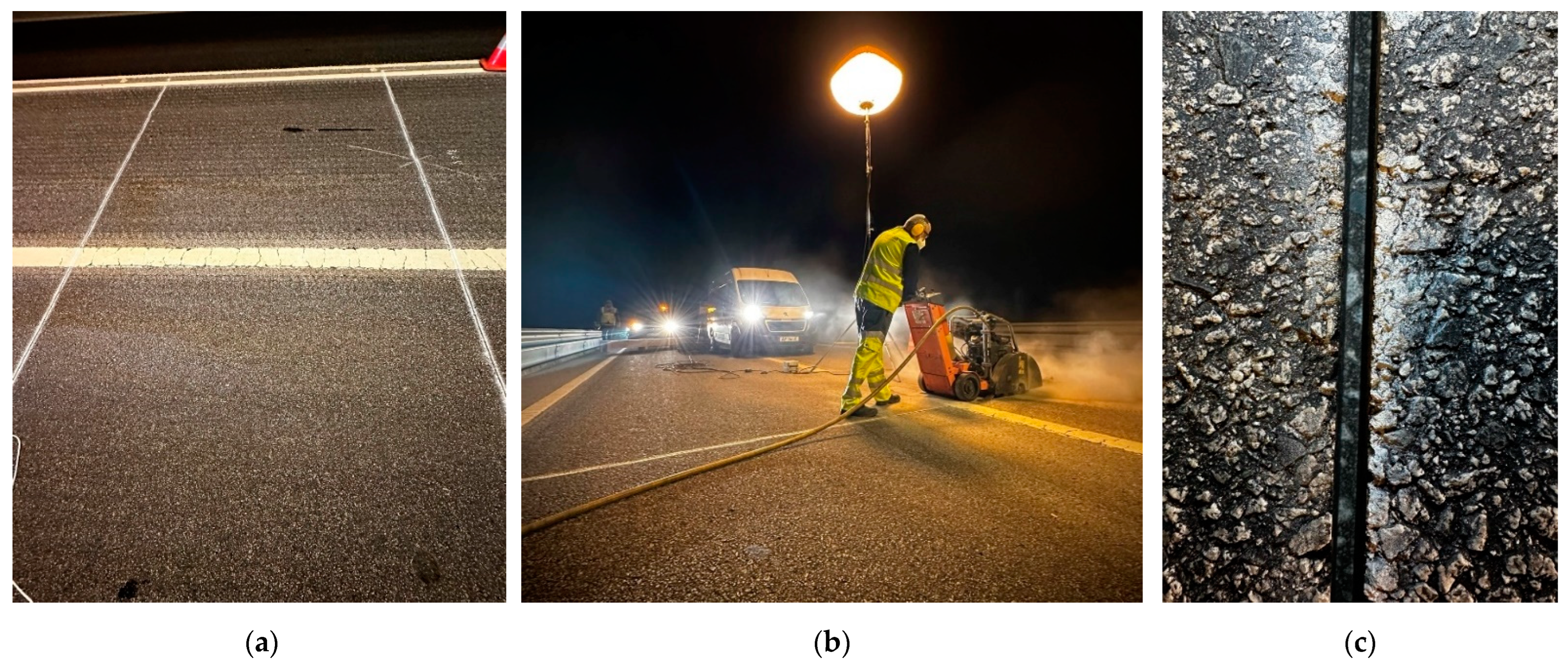
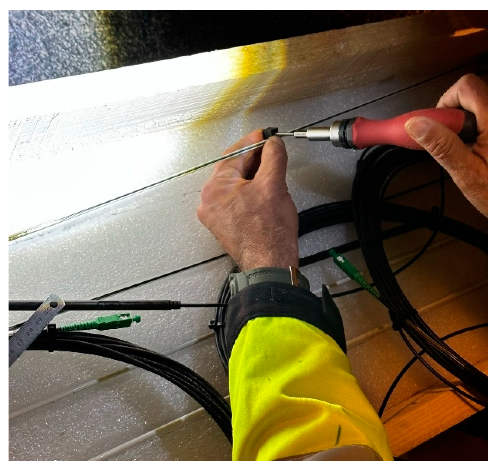
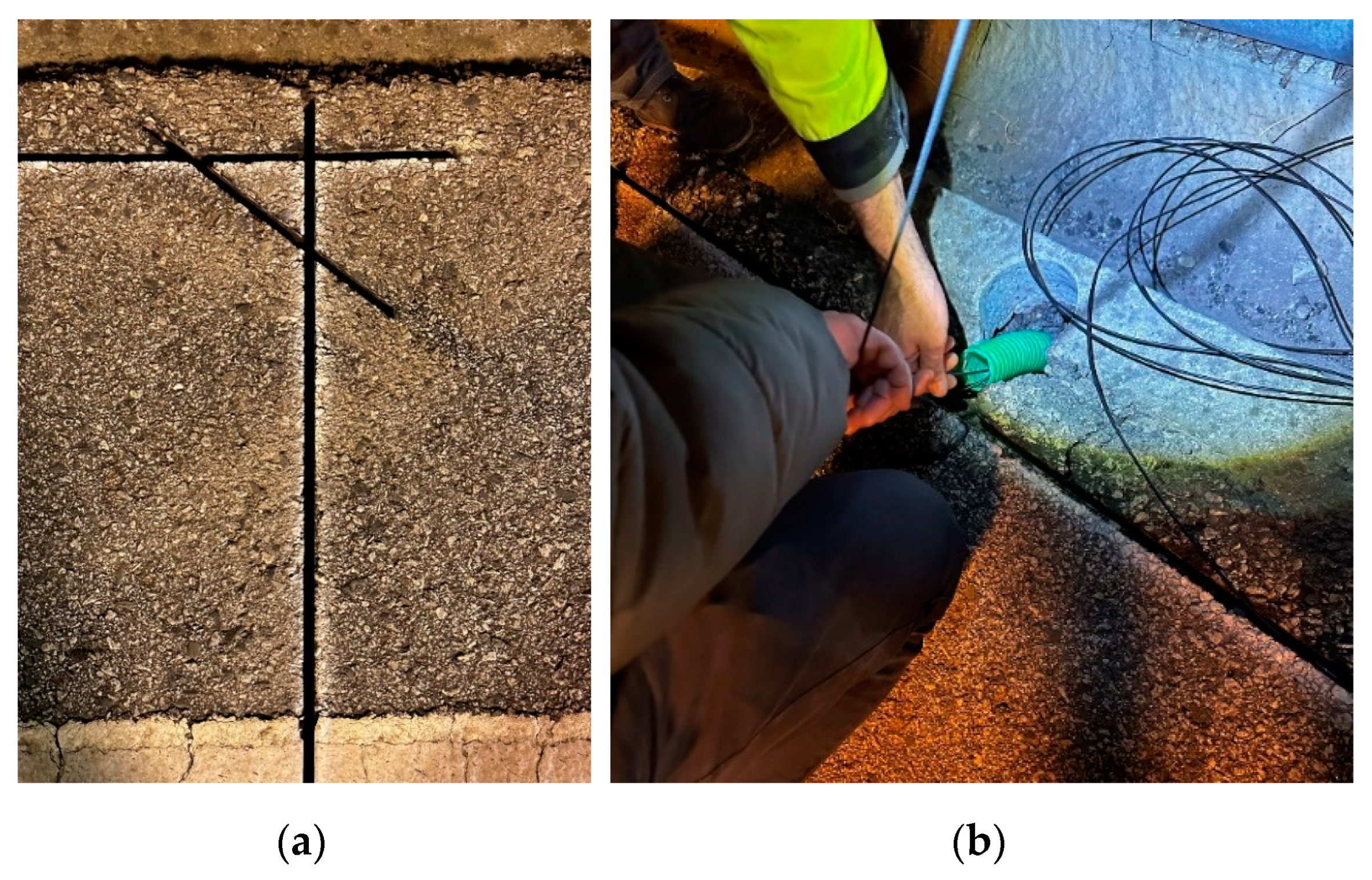
3.4. Pavement Monitoring System Installation

The research carried out in the laboratory at an early stage of this work was essential to identify the potential problems that could be faced in this application. Thus, on the one hand, the design of the monitoring system should ensure the mechanical strength necessary to withstand the vehicle loads and, on the other hand, the system should be able to assure an efficient transmission of strains/stresses between the pavement, the filling resin, and the instrumented rod. Therefore, the monitoring system was installed according to the recommendations from the laboratory study and the small trial performed at the national civil engineering laboratory. The details of the installation are given below.
First, two grooves were made in the pavement with a depth of approximately 14 cm and 3 m apart (Figure 6), where four instrumented rods of the monitoring system were later installed. Rods A1 and A2, with seven strain sensors, were installed in the first groove, while rods B1 and B2, with fifteen strain sensors, were installed in the second groove, as shown in Figure 5.
The groove depth was defined to install the sensors near the bottom of the asphalt layers where the maximum tensile strains causing fatigue cracking occur. The distance between the two grooves is essential to assess the traffic speed by knowing the elapsed time between the consecutive strain peaks measured in rod A and B sensors due to traffic. The selection of a smaller distance would have reduced the reliability of speed calculation, while higher distances could have caused some data loss due to vehicles changing lanes (e.g., during overtaking manoeuvres).
As mentioned previously, the width of the grooves was already set at 1 cm, as well as the type of resin that would be used to fill them after installing the instrumented rods. The cutting of the pavement grooves was performed without water to ensure the resin perfectly adhered to the groove and the instrumented rod. Furthermore, after the dry cutting, the groove was cleaned using an air blast to apply the resin on a dry surface free of dust and dirt, ensuring the best performance of the resin.
After cleaning the grooves, the four instrumented rods and their fibre-optic cables were installed. Considering that the grooves were cut across the entire width of both traffic lanes, two distinct rods were positioned in each groove (one on the fast traffic lane and the other on the slow traffic lane). Thus, it was necessary to overlap the fibre-optic cables of the rods on the fast (left-hand side) lane over the rods on the slow (right-hand side) lane and join the four cables on the right-hand side of the road.
In order to ensure that the fibreglass rod would not move during the resin application, several plastic fixing pieces were developed by the system supplier. These pieces were built to fit the groove width and were fixed to the rod (Figure 7) to prevent it from rotating or moving once laid, thus ensuring the sensors would be installed in the expected position.
As can be observed in Figure 8, the four cables were routed through auxiliary grooves made in the shoulder towards the corrugated pipe that connects to the technical cabinet where the interrogator was located.
After the instrumented fibreglass rods and cables had been positioned correctly in the grooves, the resin was prepared by mixing two components: a polymer compound and a hardener. Filling the grooves with resin (Figure 9a) was simple since this material has good workability and can be handled at ambient temperature. Special care was taken when overlapping fibreglass rods A2 and B2 with the cables from fibreglass rods A1 and B1, placing enough resin among them to avoid future interference in the strains to be measured on the slow (right-hand side) traffic lane.
The relatively low ambient temperature influenced the resin curing time, extending the time available for mixing, handling, and applying the resin. Therefore, filling the grooves with resin did not present any particular problems.
After filling the grooves with resin, the four cables were routed into the technical cabinet through a corrugated pipe and connected to the optical interrogator. The technical cabinet is linked to the assistance and maintenance road administration centre through an Ethernet connection, assuring the data transmission into a server for collection and subsequent analysis. Once the connection of the optical cables was finished, the first tests were carried out by the FBG sensors’ supplier (HBK company) with a portable interrogator (Figure 9b), which confirmed the excellent signal strength of the forty-four strain sensors and four temperature sensors.
The last step of the installation was the resin rectification (Figure 9c) to level the pavement surface where the two grooves were made before reopening both lanes to regular traffic. Naturally, the resin only reached the necessary hardening point for traffic reopening after a few hours due to the low ambient temperature, increasing the duration of the entire installation process. The monitoring system installation took about nine hours to complete.

3.5. Pavement Monitoring System Calibration

The data collection process began after the monitoring system based on FBG sensors was installed. After a few initial adjustments, the system continuously picked up the pavement’s strain data. Due to the high sampling rate (i.e., equal to or higher than 500 samples per second) required to record all the relevant information from dynamic loads applied on the pavement, a vast amount of data was generated that needed to be filtered, treated, and analysed.
Regarding the analysis, knowing that pavements are structures whose behaviour is influenced by various factors, a proper calibration procedure should be carried out to validate the information provided by the monitoring system and understand the performance of the pavement. This calibration procedure aims to analyse the behaviour of the pavement as a whole and, in particular, the most influential factors, such as the magnitude and position of the surface applied loads and the pavement temperature. Therefore, calibration tests were performed with a falling weight deflectometer (FWD) and based on heavy vehicles of known weights passing over the monitoring system.

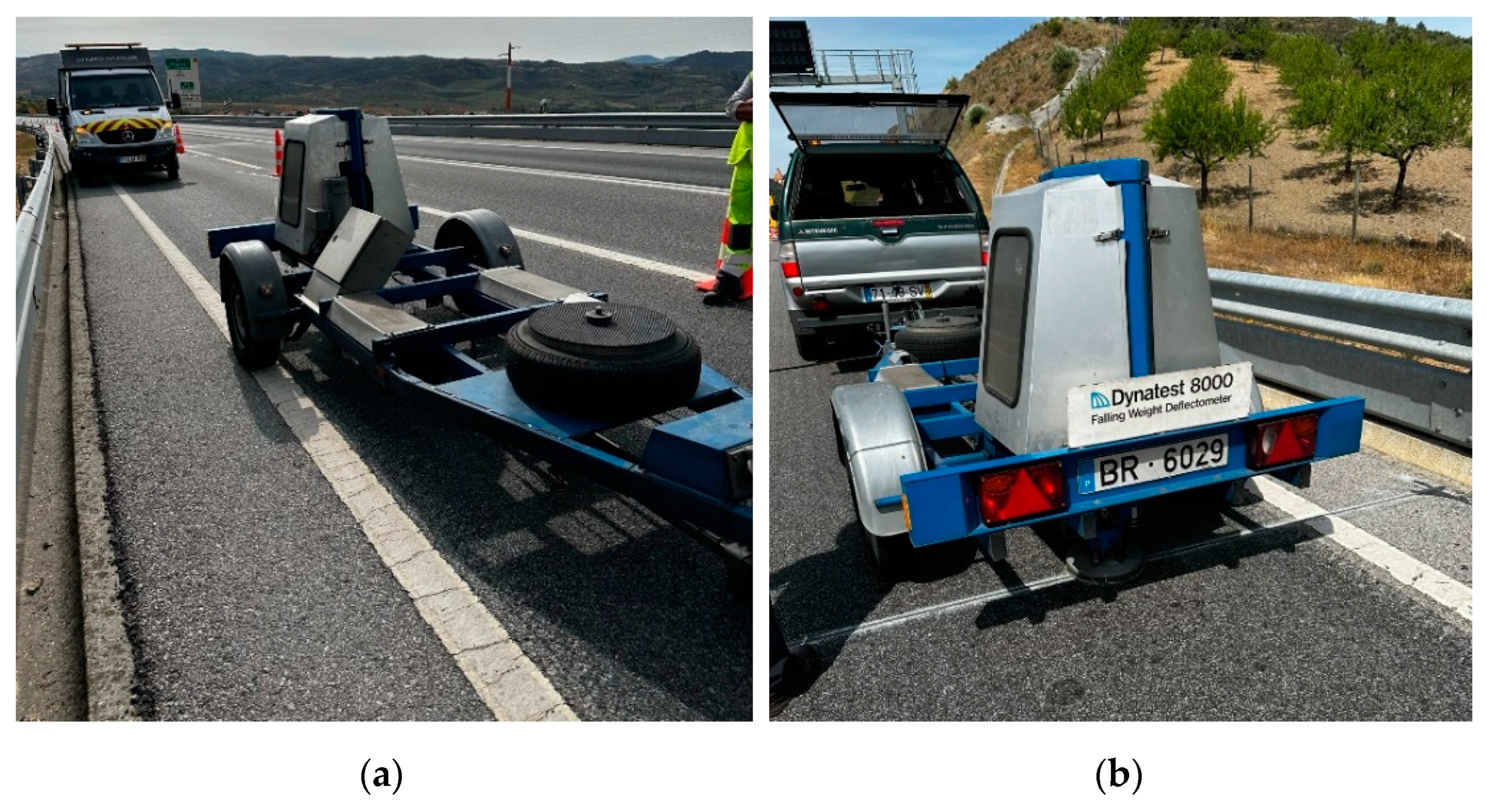
3.5.1. Calibration with Falling Weight Deflectometer Tests

The first calibration tests were performed using the falling weight deflectometer (FWD), as shown in Figure 10. The main objective of these tests was to analyse the behaviour of the pavement at different temperatures and for different load levels.
Five test campaigns were carried out throughout the day at different temperatures in this first type of calibration. Each test campaign included six positions per rod, twelve in total, where the equipment plate was laid (Figure 11). Four increasingly higher loads were applied in each position, according to the weight falling height.
The tests were performed on both instrumented rods (A2 and B2) installed on the slow (right-hand side) lane to allow the traffic to circulate in the other lane. With this procedure, it was possible to understand if the higher number of sensors in rod B2 could provide more reliable results.

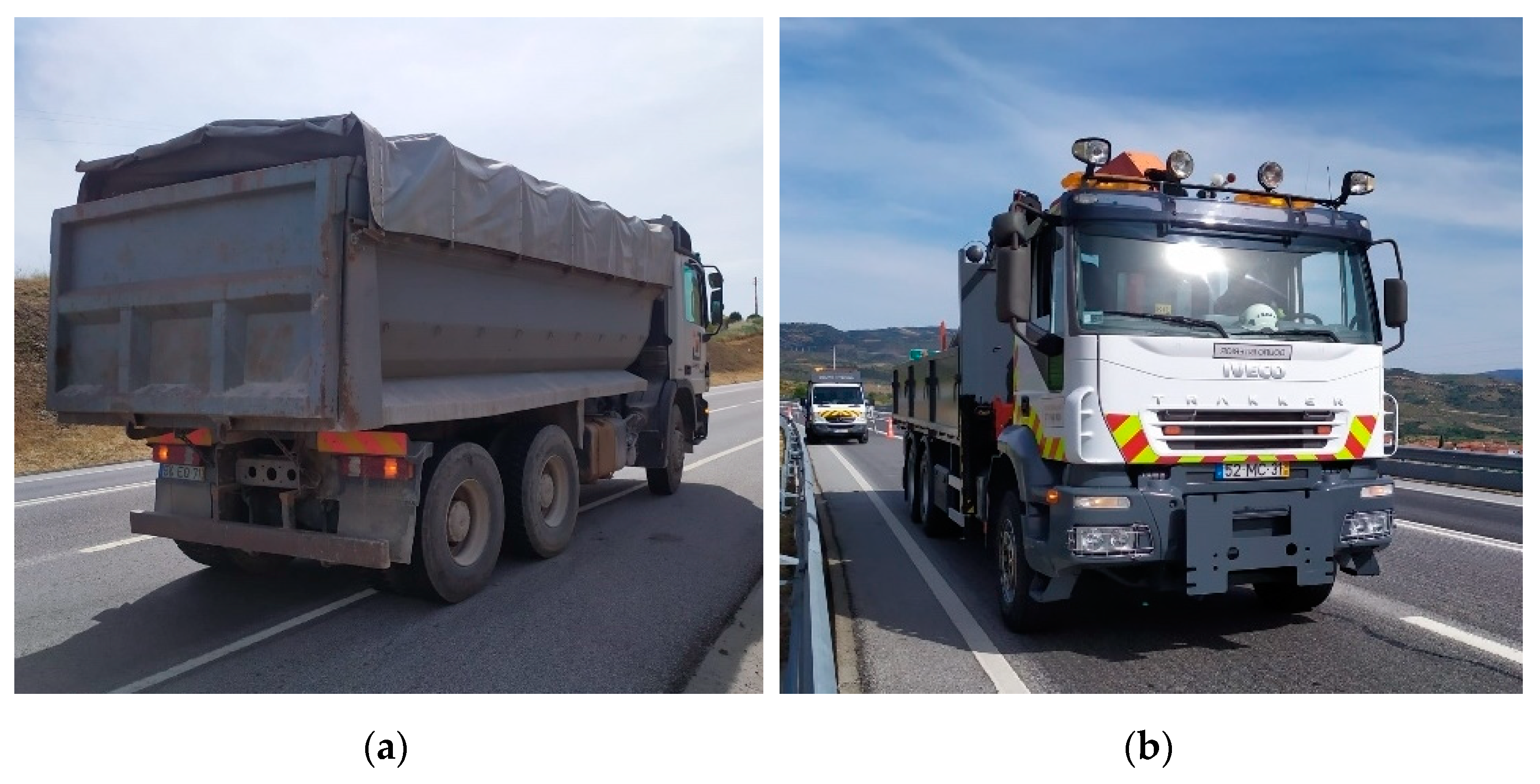
3.5.2. Calibration for Heavy Vehicles Passing with Known Loads

In addition to the tests performed with the FWD, the calibration process also aimed to study the effect of heavy vehicle loads on the pavement’s behaviour. This task used two trucks with known weights (Figure 12).
Thus, knowing the weather conditions observed during the calibration test, it is possible to establish a relationship between the strains measured on the pavement and the weight of each vehicle. Vehicles 1 and 2 had a total weight of 29.66 tons and 15.66 tons, respectively.

3.6. Analysis of the Results Obtained during the Monitoring System Calibration

The interpretation of the results obtained during the system calibration depended on the synchronisation of data obtained by different means (e.g., FWD results and strain measurements in the sensors) and the subsequent data analysis to be performed. The four instrumented rods were divided into four channels to facilitate data analysis.
The Catman software (catmanEasy version 5.6.1.12) was used to visualise the real-time strains in the FBG sensors and collect the on-site data, subsequently analysed using Matlab (version R2023a Update 3) and Microsoft Excel (for Microsoft 365 MSO version 2211 Build 16. 0. 15831. 20098) software.
The falling weight deflectometer test results and the corresponding FBG strains registered in the monitoring system were analysed to determine the amplitude of the peak strains corresponding to each load application. Temperature also plays a critical role in this analysis. The distance of each sensor to the FWD plate centre was estimated by knowing the position of the equipment in each load application, which was then used to obtain the transverse strain basins and understand the pavement behaviour.
The calibration tests performed with heavy vehicles were used to assess parameters such as the vehicle’s speed and obtain strain basins in both transverse and longitudinal directions due to the dynamic effect of the moving loads.
The pavement response under different types of axle loads is another variable that will be addressed in the results section by analysing the strain peaks caused by the passage of single- and double-wheeled axles.

4. Results and Discussion

4.1. Falling Weight Deflectometer Test Results

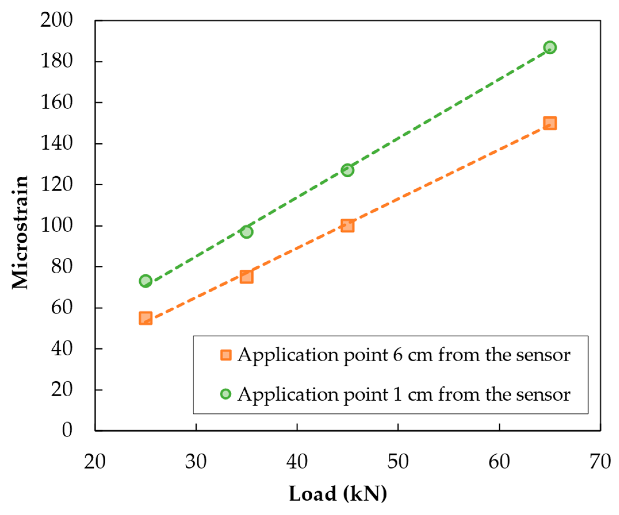
4.1.1. Sensor Sensitivity

The position of each sensor in the pavement was determined during the installation, considering the distance between the pavement marking and the beginning of the instrumented rod and the internal distance among the sensors specified in Figure 3. Thus, based on the position at which the FWD loading plate was located (Figure 11), it was possible to estimate the distance between the centre of the plate and the FBG sensors. Consequently, Figure 13 compares the maximum strain values measured when applying the 25, 35, 45, and 65 kN loads at horizontal distances of 1 cm and 6 cm from a specific sensor (measured from the centre of the FWD plate).
Increasing the distance between the load and the sensor by 5 cm causes a reduction in the maximum strain of between 20% and 25%. The results show that the pavement response, measured by the sensors’ horizontal strains, is very sensitive to the distance from which the load is applied. Thus, the number of sensors included in the instrumented rods (and the consequent internal distance) will be critical in detecting the accurate peak strain values resulting from each vehicle load application on the pavement.
Furthermore, it is possible to observe that a linear relationship exists between the strain and the load, which is discussed later in this manuscript.

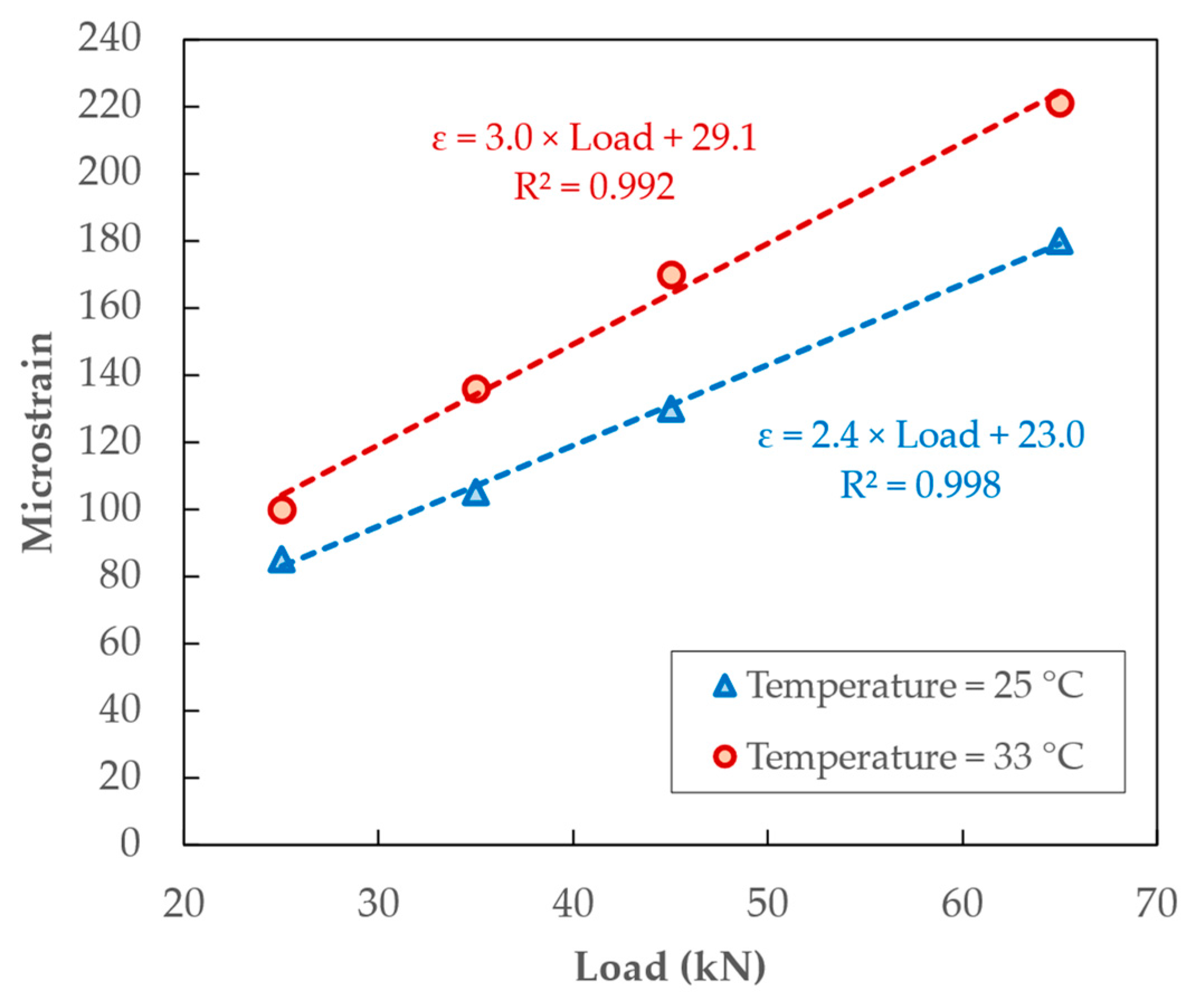
4.1.2. Temperature Influence

Several FWD tests were performed during a significant part of the day to evaluate the influence of ambient and pavement temperature on the strain level measured by the FBG sensors embedded in the pavement under different weather conditions. This information is essential for asphalt pavements since they exhibit viscoelastic behaviour and are susceptible to temperature and loading frequency.
Figure 14 presents the maximum strain values measured by the monitoring system in sensor 5 of rod A2 for FWD tests performed in position E (Figure 11) to exemplify the strain variation with temperature. The horizontal distance between sensor 5 of rod A2 and the FWD load application point E is approximately 2 cm. The lowest pavement temperature registered by the monitoring system during the FWD calibration tests was 25 °C, measured at 11:00 a.m., and the highest temperature registered during those tests was 33 °C at 4:30 p.m. Thus, Figure 14 compares the maximum strain values measured when applying the 25, 35, 45, and 65 kN loads at two testing temperatures (i.e., 25 °C and 33 °C) measured by the FBG temperature sensor of the monitoring system.
Pavements can accumulate large amounts of thermal energy from solar radiation, which may cause significant daily and annual temperature variations that influence pavement performance. This study measured a pavement temperature variation of 8 °C at a depth of about 13.5 cm from 11:00 a.m. to 4:30 p.m.
The load influence on the maximum strain values measured by the monitoring system was fitted through linear equations at both test temperatures. On average, for loads between 25 kN and 65 kN, the mentioned temperature rise of 8 °C caused an increase of about 20.3% in the horizontal tensile strains measured in the pavement. Therefore, FBG sensors are sensitive to pavement performance changes at different temperatures.

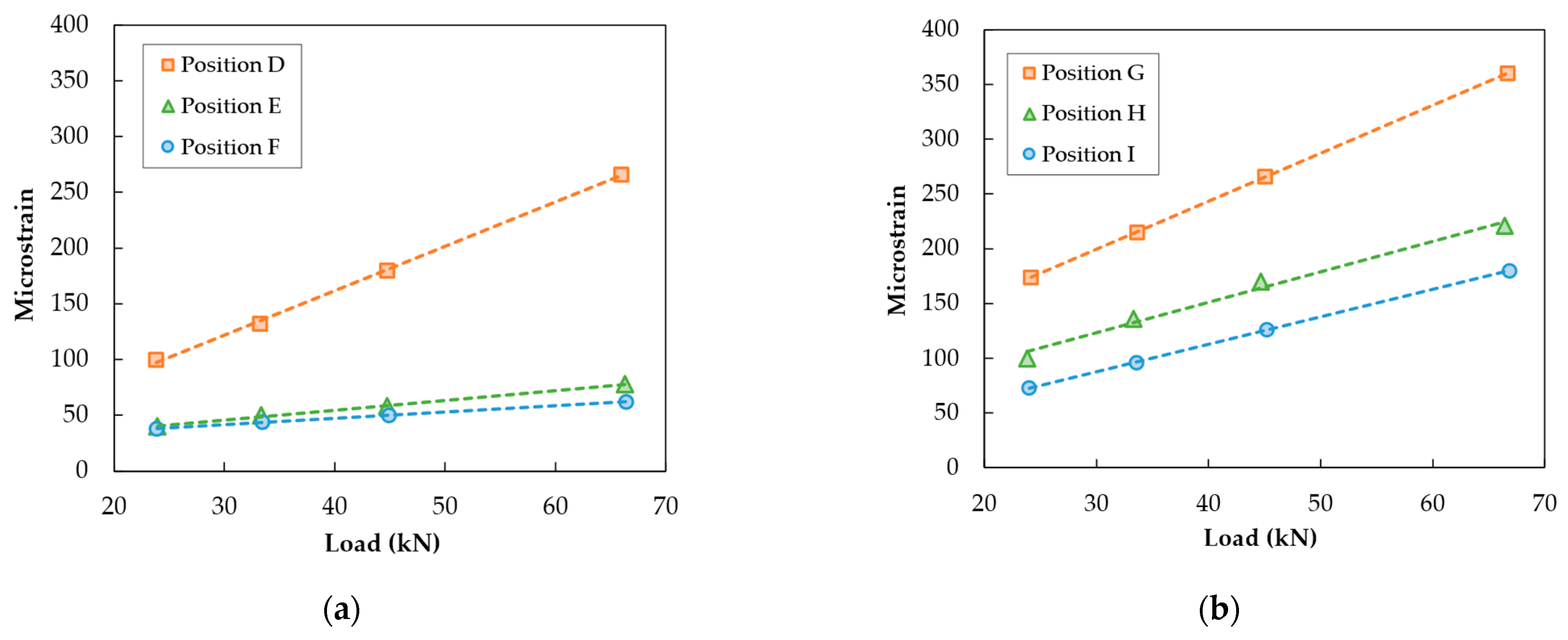
4.1.3. Relationship between Loads and Strains

All the loads (25, 35, 45, and 65 kN) applied in the twelve positions shown in Figure 11 were analysed for all the FWD test repetitions carried out throughout the day to study the evolution of the pavement strains with increasing loads.
Figure 15 shows the peak strain values measured by the monitoring system for six loading positions when the highest pavement temperature was recorded. Figure 15a concerns the loads applied on positions D, E, and F of rod A2, while Figure 15b concerns the loads applied on positions G, H, and I of rod B2.
As can be concluded from the results shown in Figure 15, there is an evident linear variation in the strains with the load applied in all situations. However, the distance from the centre of the loading plate to the closest sensors varies, influencing the evolution of the strain values obtained for the different loads. The load applied in position G is very close to the vertical alignment of sensor 2 on rod B2, while the distance of the closest sensor to the centres of the load in positions H (sensor 5) and I (sensor 7) is 3 cm and 4 cm, respectively. Many factors influence the strains recorded in pavements due to their complex behaviour, and sensors placed in diverse pavement locations may present different strain values under similar loading conditions. Nevertheless, a decrease in the strain value measured in the sensor is generally associated with a higher distance to the centre of the load, as can be seen in the three mentioned positions and as previously discussed.
Although it is possible to see a linear relationship between load and strain, positions E and F showed a marginal increase between the various loads applied. This result can be explained by the horizontal distance from the load application point to the closest sensor of rod A2. In position D, the load centre is vertically aligned with sensor 4; position E represents a distance of 15 cm between the centre of the plate and sensor 5; finally, position F represents a distance of 21 cm between the centre of the plate and sensor 6. Despite the slight variation in the strains measured for the last two positions, they always increase with the load applied on the pavement surface, which is satisfactory. The results highlight the importance of the distance between the sensor and the position where the load is applied if the load value is to be estimated.

4.1.4. Transverse Strain Basins

The loading effect of traffic on road pavement, also simulated by the FWD tests, causes changes in its stress and strain state response noted up to a certain distance from the load application position. Therefore, the multiple sensors of the monitoring system were used in this work to evaluate the transverse strain basins resulting from loads applied by the falling weight deflectometer in specific positions.
Initially, Figure 16a represents the strain variation over time measured in sensor 2 of fibreglass rod A2 for a 65 kN load applied with the FWD in position B (14 cm apart). Figure 16b shows a similar result registered in sensor 5 of fibreglass rod B2 for the same load applied in position H (2 cm apart).
The dynamic effect of the falling weight load on the pavement response is evident in these results because FBG sensors could register the strains caused by the several rebounds of the weight on the pavement. The maximum strain recorded in sensor 2 of rod A2 was 145 με, while the maximum strain measured in sensor 5 of rod B2 was 182 με. The smaller distance between the loading position H and sensor 5 justifies the increased strain values measured in that sensor. Thus, on average, the fibreglass rods with fifteen sensors (B1 and B2) are expected to measure higher peak strain values than those with seven sensors (A1 or A2) because the distance from a random traffic load position to the nearest sensor will be statistically lower when using more sensors in the monitoring system.
Subsequently, Figure 17 presents the maximum strain values measured in all the FBG sensors of each rod (A2 and B2) for the 65 kN load applied in positions B and H, respectively. The points represent the strain values registered in each sensor, and the line connecting these points can be described as the transverse strain basin.
In fibreglass rod A2 (in brown), with seven sensors, only sensor 2 (the second value from the right-hand side) recorded tensile (positive) strains because it was nearest to the load application point. The adjacent sensors (1 and 3) registered compression strains because they were 36 cm and 64 cm away from the load application point. These compression strains are expected to occur adjacent to the tyre loads in the bottom part of the asphalt layers, as described by Sudarsanan and Kim [31].
Regarding fibreglass rod B2 (in green), with more sensors, three sensors (4, 5, and 6) registered tensile (positive) strains. The difference that an increase in the number of sensors causes in the results, namely in the strain basin shape, is significant, improving the understanding of the actual pavement response to load applications. In this case, sensor 4 was 13 cm away, sensor 5 was 2 cm away, and sensor 6 was 17 cm away from the centre of the loading plate. The shorter distance between sensors 4, 5, and 6 of rod B2 also allowed a more precise definition of the strain peak than rod A2 (sensor 2), measuring a strain value 24% higher than rod A2.
The higher number of sensors included in rods B1 and B2 will be of great value in the comprehensive characterisation of the pavement performance over time. The more detailed strain basins also allow a better understanding of the compressive (negative) strains generated in the regions surrounding the loaded area of the pavement, which is not adequately characterised by the rods with fewer sensors due to the higher distances among the sensors. However, those rods with fewer sensors are essential to evaluate the traffic speed, as explained later in this manuscript, which affects the pavement response.

4.2. Results from the Dynamic Loading Effect of Heavy Vehicles

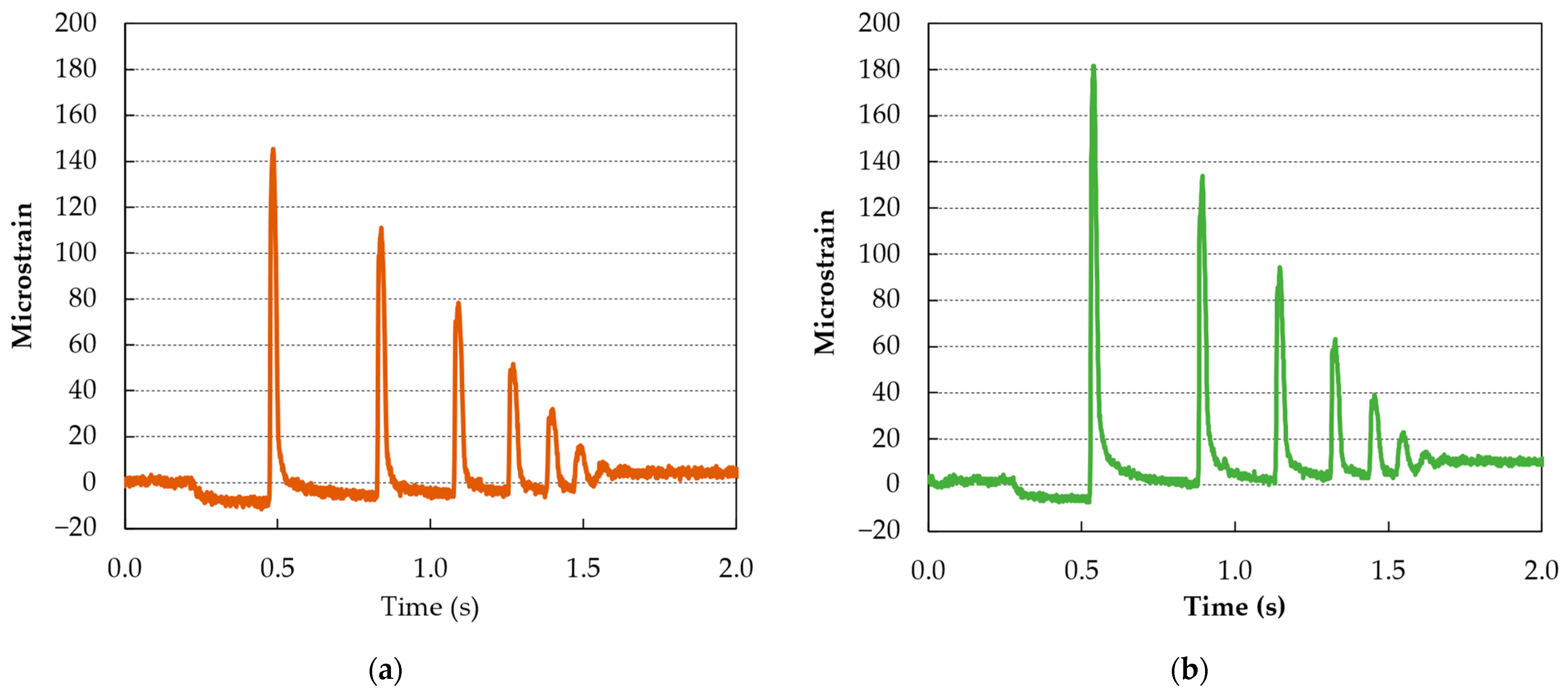
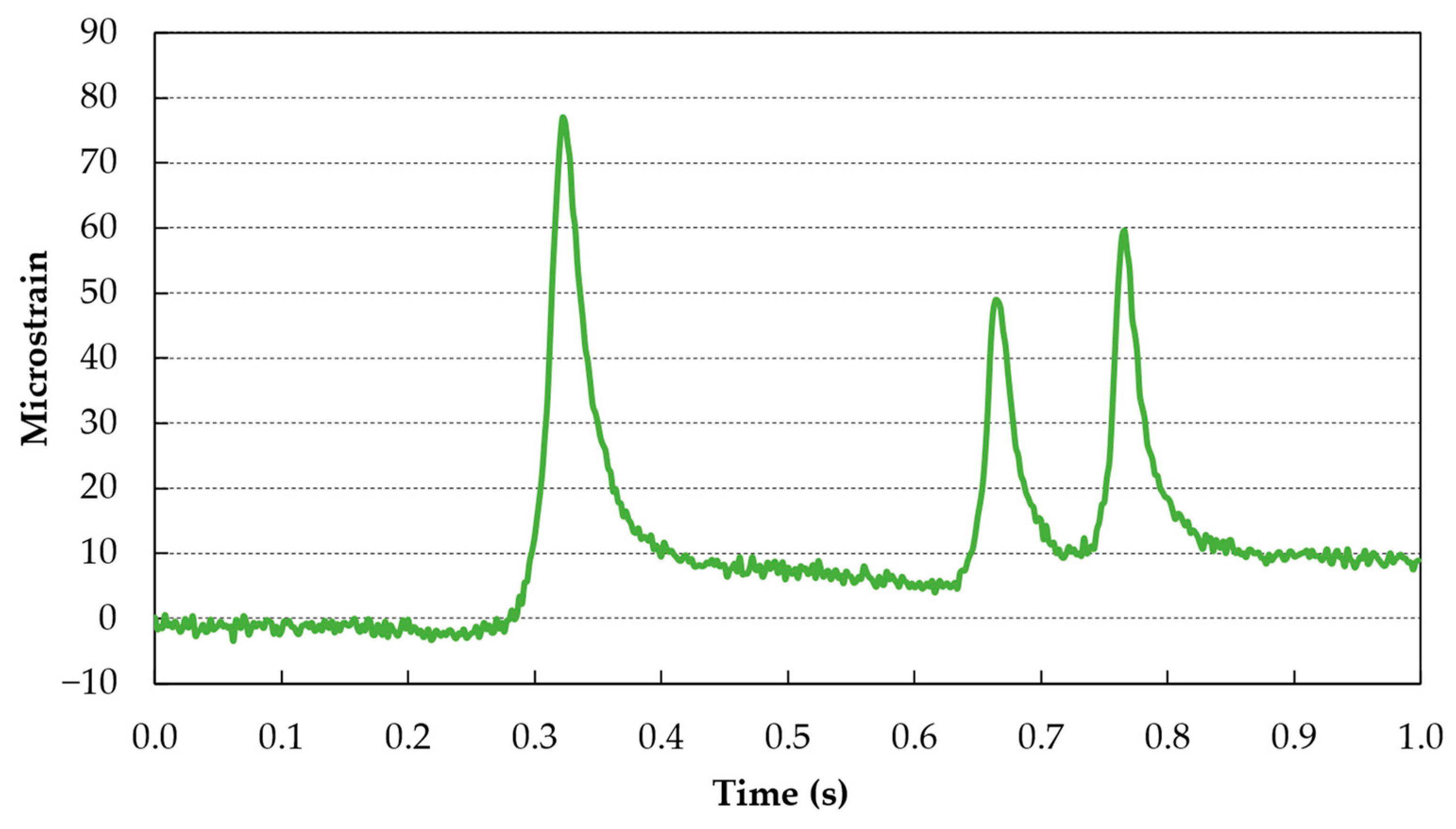
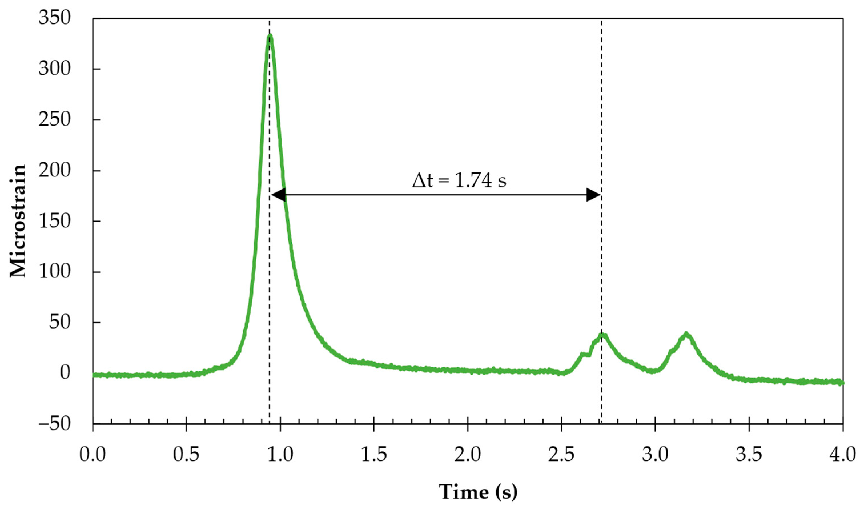
4.2.1. Strains Caused by Heavy Vehicles

Figure 18 shows the strains caused by the passage of Heavy Vehicle 1, registered in sensor 6 of rod B1. This vehicle has a total mass of 29.66 tons, distributed over three axles (a single-wheeled front axle and two double-wheeled rear axles).
As can be seen from the graph, the front axle caused more significant strain than the rear axles, which may be related to the higher load distribution enabled by the rear axles that are close to each other and both of which possess a double-wheeled configuration, thus assuring a larger contact area between the tyres and the pavement and a lower stress applied to the surface. Among the rear axles, the last axle also caused peak strains higher than the first one, which is explained by the viscoelastic behaviour of the asphalt pavement, where the time between loads of both axles is not enough to allow the pavement to fully recover from the deformation (strain) imposed by the first axle before the load of the second axle is applied.
The vehicle speed calculation (Figure 19) considers the distance between the two instrumented rods (3 m) and the time it takes for one axle to be recorded by rod A1 (first peak in the graph) and rod B1 (second peak), which in this case is 0.204 s. Thus, as demonstrated in Equation (5), the speed of this truck (Vehicle 1) was 52.9 km/h.
s = d t = 3   m 0.204   s = 14.7   m / s = 52.9   km / h
Figure 20 shows the strains caused by Heavy Vehicle 2 in one of its passages over the monitoring system and registered by sensor 3 of rod B2. These graphs can be used to estimate the distance between the vehicle’s axles after computing the vehicle speed.
Using the same method presented previously in Figure 19 for Vehicle 1, the average speed of Vehicle 2 was calculated to be approximately 9.8 km/h. At that speed, it took about 1.74 s for the first and second axles to cross the same instrumented rod. Therefore, these values make it possible to determine that the distance between the first and second axles of Vehicle 2 is 4.74 metres.
This vehicle did not carry any significant load, which may explain that, unlike Vehicle 1, there was no increase in the strains from the first to the second rear axle. Furthermore, the vehicle’s low speed (circulating in a protected area) allows the pavement to recover from the deformation caused by the passage of the previous axle. In addition, as in Vehicle 2, the rear axles are double, leading to better weight distribution and consequently, the peak strains measured when those axles pass over the system are significantly lower than those observed for the front axle.

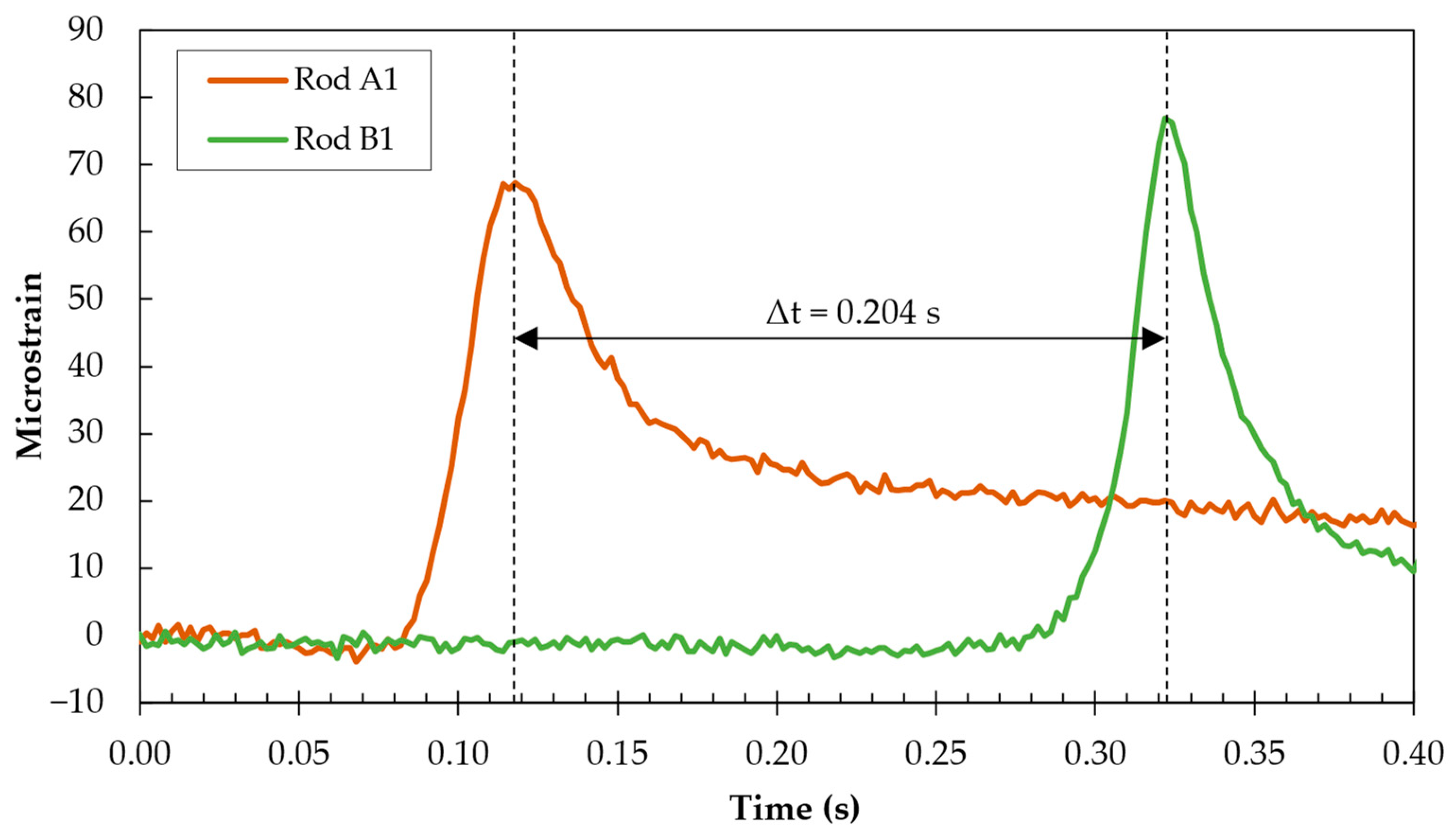
4.2.2. Influence of the Type of Axle on the Strain Lateral Distribution

Both heavy vehicles have three axles (one front and two rear axles), and in both situations, the two rear axles are double-wheeled, and the front axle is simple. Thus, this analysis was only performed for Vehicle 2. Although the actual weight of each axle was unknown, the total weight of this vehicle was 15.66 tons.
Figure 21 presents the maximum strains recorded by the monitoring system when the front single-wheeled axle and first rear double-wheeled axle of Vehicle 2, respectively, passed over the fifteen sensors of fibreglass rod B2.
As observed in these graphs, it is possible to identify the sensors most loaded by both wheels and determine the lateral distribution of the vehicle loads. In this case, sensors 2 and 3 of Figure 21a relate to the left wheel, and sensors 11 and 12 to the right wheel of the front axle. This single-wheeled axle produced positive strains in an area with a radius of approximately 15 cm (spacing between the two sensors).
The first rear axle of this heavy-duty vehicle is shown in Figure 21b. By comparison with Figure 21a, it is possible to understand the different pavement behaviour under these double-wheeled axle loads. This axle type causes four sensors to register positive strain values for each set of wheels, resulting in an approximately 60 cm diameter area of tensile strain under the wheels. The increased load distribution area justifies the significantly lower strain values registered for the rear axle.

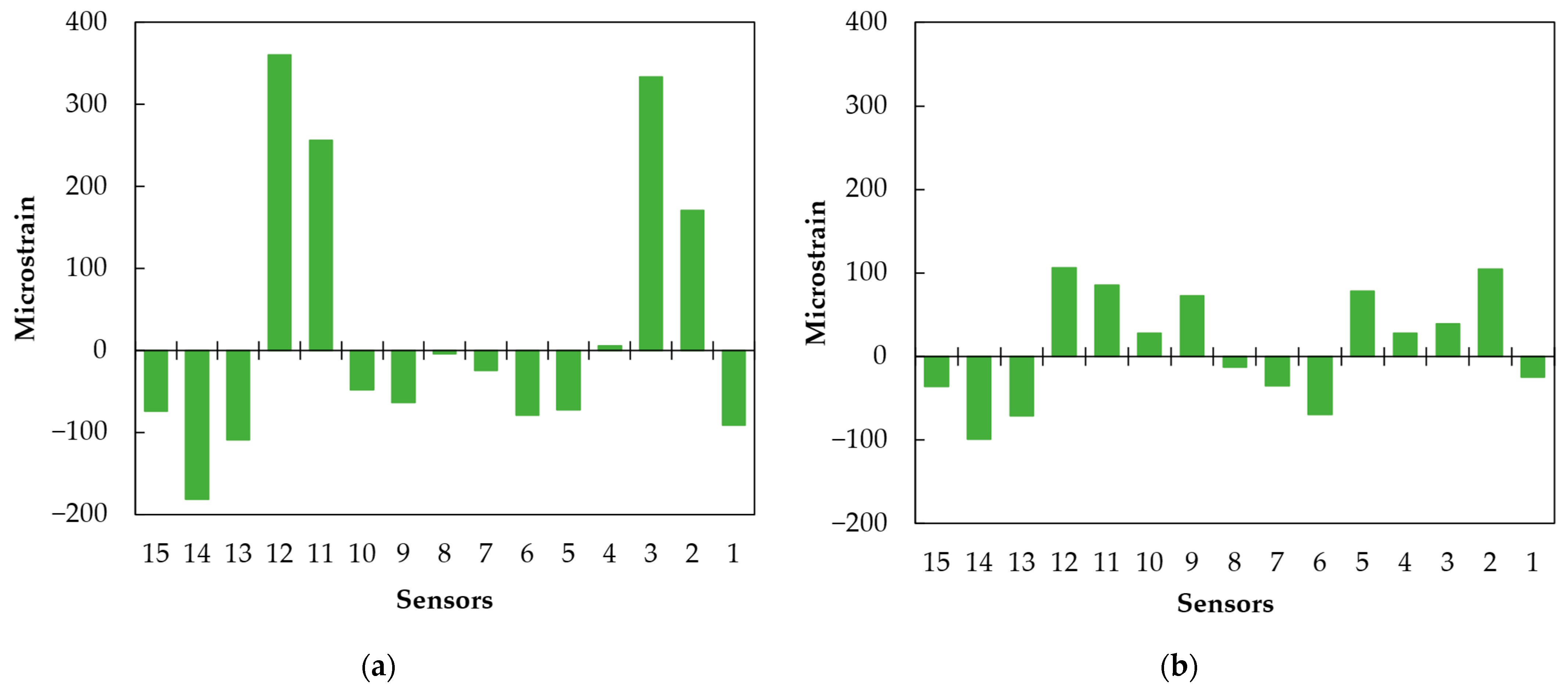
4.2.3. Transverse and Longitudinal Deformation Basins

An overview of the horizontal strains measured in the transverse direction caused by the three axles of Vehicles 1 and 2 is shown in Figure 22 and Figure 23.
The 3D graph allows a global visualisation of the information collected in all FBG sensors of each rod (B1 and B2), providing a more comprehensive perspective of the strains imposed in that pavement section over the period during which the vehicle passage was recorded. This type of analysis focuses more on evaluating the loading effect of the passing vehicle on the pavement response according to the observed weather conditions.
In this graph, it is possible to observe the compressive (negative) strains generated in the areas adjacent to those loaded by the vehicle wheels. On the other hand, comparing the deformation (strain level) before and after the front axle loads are applied, it is clear that the pavement deformation imposed by these loads has a delayed recovery, typical of asphalt materials, due to their viscoelastic nature.
Figure 23 shows the difference in the results obtained between axles with single and double wheels, with a considerably higher loaded area in the rear axles of the heavy vehicle. Despite circulating over the monitoring system with a much lower load than Vehicle 1, Vehicle 2 caused significantly higher strains in all axles. As previously demonstrated, its speed was much lower, influencing the results obtained by the monitoring system. Slower loading frequencies result in a lower stiffness modulus of the asphalt layers, which implies the development of higher strain levels within the pavement structure. Furthermore, Vehicle 2 circulated in the slow traffic lane, whose pavement may have a lower bearing capacity than the fast traffic lane (where the passage of Vehicle 1 was registered), as usually occurs due to the increased damage caused in the pavement by heavy and low-speed loads typically passing in the slow traffic lane.
This analysis with 3D graphs may be a valuable tool in studying pavement performance evolution over time. Furthermore, it can be used to analyse the effects of different axle and vehicle configurations on pavement behaviour, including the effect of pavement temperature and vehicle speed, and help improve the pavement performance models used to schedule pavement maintenance operations.

5. Conclusions

The process of installing a continuous pavement monitoring system based on FBG optical sensors presented here, along with a series of calibration tests performed in the following weeks, allowed some conclusions regarding its operation to be drawn:
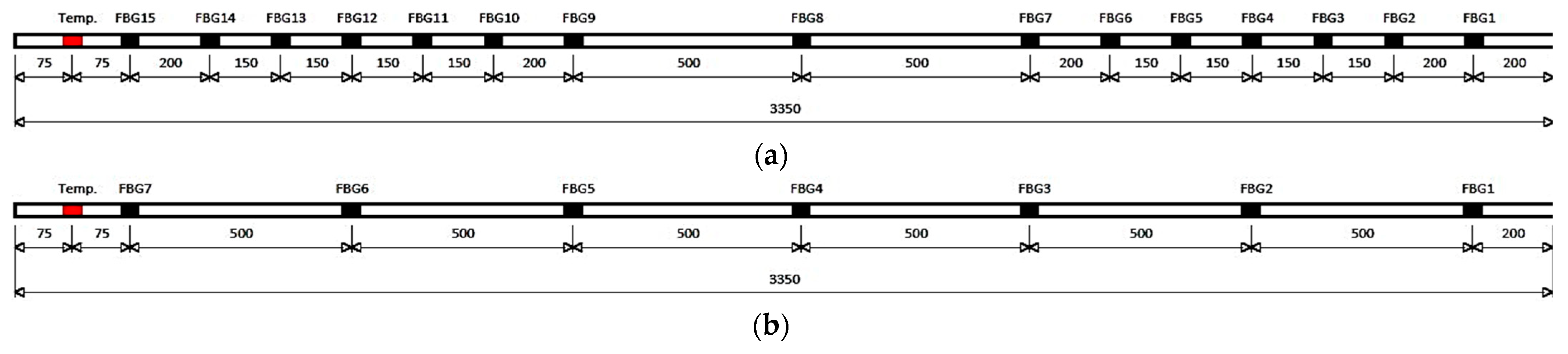
  • The type of sensors used in this work is very accurate; slight differences in the position of the load (in the order of 50 mm) may cause significant differences (20% to 25%) in the strains obtained for the same load, justifying the shorter distances (150 mm) between the sensors used in two of the instrumented rods, namely near the wheel tracks;
  • One of this technology’s critical issues is the temperature calibration of the sensors, as they are susceptible to temperature variations. However, a calibration factor can be applied to each sensor to correct the readings using the software (Catman) provided by the supplier of the sensors. Moreover, it was observed that a temperature rise of 8 °C increased the measured tensile strains by about 20%;
  • The FWD tests performed with different loads for calibration of the monitoring system showed that a linear relationship could be established between the applied load and the strains obtained, which will be used in the future to analyse the data gathered from this monitoring system, to estimate the loads applied to the pavement surface;
  • The effects of the type and number of axles of each vehicle on the response of the pavement at each load application were analysed in this work, using 3D representations of the strains over time; the fibreglass rods instrumented with 15 strain sensors were essential for the accurate representation of this information, yielding reliable knowledge of the pavement behaviour;
  • The rods instrumented with 15 strain sensors provide a more comprehensive analysis of the transverse variation in the strains in a pavement section, which can be associated with the temperature data measured by the specific sensors installed for that purpose to assess the evolution of the pavement performance over its lifecycle, generating valuable information to develop pavement performance models.
The main limitation of this study is the lack of universality among the calibration results due to restrictions in the time available to perform the tests, as these experiments demanded the road’s closure, which could only be possible during a short period. Thus, only four FWD loads could be applied to the pavement in each testing location, and the temperature variations only represent a small spectrum of the whole range values observed in this location in a day or a year.
Briefly, this monitoring sensor technology will be used as a monitoring technology to assess pavement performance by measuring variations in the pavement response to load application during the different seasons and throughout the pavement’s life. Nevertheless, at this stage of software development, using the collected traffic data to estimate the average load per vehicle is still not viable with this system.

Author Contributions

Conceptualisation, F.J.P.R., J.R.M.O., H.M.R.D.S., J.O.e.S., V.M. and J.A.; methodology, F.J.P.R., J.R.M.O., H.M.R.D.S., J.O.e.S., V.M. and J.A.; validation, J.R.M.O. and H.M.R.D.S.; formal analysis, V.M., J.R.M.O. and H.M.R.D.S.; investigation, F.J.P.R., J.R.M.O., H.M.R.D.S., J.O.e.S., V.M. and J.A.; writing—original draft preparation, F.J.P.R., J.R.M.O., H.M.R.D.S. and J.O.e.S.; writing—review and editing, F.J.P.R., H.M.R.D.S. and J.R.M.O.; supervision, J.R.M.O., H.M.R.D.S. and J.O.e.S. All authors have read and agreed to the published version of the manuscript.

Funding

This research was funded by PORTUGAL 2020 through the Operational Program for Competitiveness and Internationalization (POCI) and the European Regional Development Fund (ERDF) under the project “Rev@Construction—Digital Construction Revolution”, with reference POCI-01-0247-FEDER-046123, and by Fundação para a Ciência e a Tecnologia through the PhD grant number 2022.14400.BD. This work was also partly financed by FCT/MCTES through national funds (PIDDAC) under the R&D Unit Institute for Sustainability and Innovation in Structural Engineering (ISISE), reference UIDB/04029/2020, the Associate Laboratory Advanced Production and Intelligent Systems ARISE, reference LA/P/0112/2020, and the R&D Unit ALGORITMI, reference UIDB/00319/2020.

Institutional Review Board Statement

Not applicable.

Informed Consent Statement

Not applicable.

Data Availability Statement

Data sharing does not apply to this article.

Acknowledgments

The authors would like to acknowledge the staff from the authors’ organisations involved in this work, who contributed to achieving the objectives of this study.

Conflicts of Interest

The authors declare no conflict of interest. The funders had no role in the study’s design; in the collection, analyses, or interpretation of data; in the writing of the manuscript; or in the decision to publish the results.

References

  1. Chen, J.; Dan, H.; Ding, Y.; Gao, Y.; Guo, M.; Guo, S.; Han, B.; Hong, B.; Hou, Y.; Hu, C.; et al. New innovations in pavement materials and engineering: A review on pavement engineering research 2021. J. Traffic Transp. Eng. (Engl. Ed.) 2021, 8, 815–999. [Google Scholar] [CrossRef]
  2. Kara De Maeijer, P.; Voet, E.; Windels, J.; Van den Bergh, W.; Vuye, C.; Braspenninckx, J. Fiber Bragg grating monitoring system for heavy-duty pavements. In Proceedings of the 7th Euroasphalt & Eurobitume Congress, Virtual, 16–18 June 2021. [Google Scholar]
  3. Ai, C.; Rahman, A.; Xiao, C.; Yang, E.; Qiu, Y. Analysis of measured strain response of asphalt pavements and relevant prediction models. Int. J. Pavement Eng. 2017, 18, 1089–1097. [Google Scholar] [CrossRef]
  4. Hou, Y.; Li, Q.; Zhang, C.; Lu, G.; Ye, Z.; Chen, Y.; Wang, L.; Cao, D. The State-of-the-Art Review on Applications of Intrusive Sensing, Image Processing Techniques, and Machine Learning Methods in Pavement Monitoring and Analysis. Engineering 2021, 7, 845–856. [Google Scholar] [CrossRef]
  5. Braunfelds, J.; Senkans, U.; Skels, P.; Janeliukstis, R.; Salgals, T.; Redka, D.; Lyashuk, I.; Porins, J.; Spolitis, S.; Haritonovs, V.; et al. FBG-Based Sensing for Structural Health Monitoring of Road Infrastructure. J. Sens. 2021, 2021, 8850368. [Google Scholar] [CrossRef]
  6. Sebaaly, P.; Tabatabaee, N.; Kulakowski, B.; Scullion, T. Instrumentation for Flexible Pavements—Field Performance of Selected Sensors, Volume 1: Final Report; Pennsylvania Transportation Institut: University Park, PA, USA, 1992. [Google Scholar]
  7. Huff, R.; Berthelot, C.; Daku, B. Continuous primary dynamic pavement response system using piezoelectric axle sensors. Can. J. Civ. Eng. 2011, 32, 260–269. [Google Scholar] [CrossRef]
  8. Duong, N.S.; Blanc, J.; Hornych, P.; Bouveret, B.; Carroget, J.; Le Feuvre, Y. Continuous strain monitoring of an instrumented pavement section. Int. J. Pavement Eng. 2019, 20, 1435–1450. [Google Scholar] [CrossRef]
  9. Liu, H.; Ge, W.; Pan, Q.; Hu, R.; Lv, S.; Huang, T. Characteristics and analysis of dynamic strain response on typical asphalt pavement using Fiber Bragg Grating sensing technology. Constr. Build. Mater. 2021, 310, 125242. [Google Scholar] [CrossRef]
  10. Tan, Y.Q.; Wang, H.-P.; Sun, Z.-J.; Li, Y.-W.; Shi, X. Calibration method of FBG sensor based on asphalt pavement indoor small size test. In Proceedings of the 2011 International Conference on Transportation, Mechanical, and Electrical Engineering (TMEE), Changchun, China, 16–18 December 2011; pp. 1390–1394. [Google Scholar]
  11. Frank, M.H.; Jason, K.R.; Peter, D.F. A strain-isolated fibre Bragg grating sensor for temperature compensation of fibre Bragg grating strain sensors. Meas. Sci. Technol. 1998, 9, 1163. [Google Scholar] [CrossRef]
  12. Song, M.; Lee, S.B.; Choi, S.S.; Lee, B. Simultaneous Measurement of Temperature and Strain Using Two Fiber Bragg Gratings Embedded in a Glass Tube. Opt. Fiber Technol. 1997, 3, 194–196. [Google Scholar] [CrossRef]
  13. Patrick, H.J.; Williams, G.M.; Kersey, A.D.; Pedrazzani, J.R.; Vengsarkar, A.M. Hybrid fiber Bragg grating/long period fiber grating sensor for strain/temperature discrimination. IEEE Photonics Technol. Lett. 1996, 8, 1223–1225. [Google Scholar] [CrossRef]
  14. Jaehoon, J.; Hui, N.; Namkyoo, P.; Byoungho, L. Simultaneous measurement of strain and temperature using a single fiber Bragg grating written in an erbium:ytterbium-doped fiber. In Proceedings of Technical Digest. Summaries of Papers Presented at the Conference on Lasers and Electro-Optics. Postconference Edition. CLEO ’99. Conference on Lasers and Electro-Optics (IEEE Cat. No.99CH37013), 28 May 1999; IEEE: Piscataway, PA, USA, 1999; p. 386. [Google Scholar]
  15. Wang, H.-P.; Dai, J.-G.; Wang, X.-Z. Improved temperature compensation of fiber Bragg grating-based sensors applied to structures under different loading conditions. Opt. Fiber Technol. 2021, 63, 102506. [Google Scholar] [CrossRef]
  16. Leal-Junior, A.G.; Díaz, C.A.R.; Frizera, A.; Marques, C.; Ribeiro, M.R.N.; Pontes, M.J. Simultaneous measurement of pressure and temperature with a single FBG embedded in a polymer diaphragm. Opt. Laser Technol. 2019, 112, 77–84. [Google Scholar] [CrossRef]
  17. Han, D.; Liu, G.; Xi, Y.; Zhao, Y. Theoretical analysis on the measurement accuracy of embedded strain sensor in asphalt pavement dynamic response monitoring based on FEM. Struct. Control Health Monit. 2022, 29, e3140. [Google Scholar] [CrossRef]
  18. Liu, Z.; Gu, X.; Wu, C.; Ren, H.; Zhou, Z.; Tang, S. Studies on the validity of strain sensors for pavement monitoring: A case study for a fiber Bragg grating sensor and resistive sensor. Constr. Build. Mater. 2022, 321, 126085. [Google Scholar] [CrossRef]
  19. Rebelo, F.; Dabiri, A.; Silva, H.; Oliveira, J. Laboratory Investigation of Sensors Reliability to Allow Their Incorporation in a Real-Time Road Pavement Monitoring System. In Proceedings of the 3rd ISIC International Conference on Trends on Construction in the Post-Digital Era, Guimarães, Portugal, 26–29 September 2022; pp. 490–501. [Google Scholar]
  20. Barrias, A.; Casas, J.R.; Villalba, S. A Review of Distributed Optical Fiber Sensors for Civil Engineering Applications. Sensors 2016, 16, 748. [Google Scholar] [CrossRef]
  21. Majumder, M.; Gangopadhyay, T.K.; Chakraborty, A.K.; Dasgupta, K.; Bhattacharya, D.K. Fibre Bragg gratings in structural health monitoring—Present status and applications. Sens. Actuators A Phys. 2008, 147, 150–164. [Google Scholar] [CrossRef]
  22. Lei, Y.; Hu, X.; Wang, H.; You, Z.; Zhou, Y.; Yang, X. Effects of vehicle speeds on the hydrodynamic pressure of pavement surface: Measurement with a designed device. Measurement 2017, 98, 1–9. [Google Scholar] [CrossRef]
  23. Hottinger Bruel & Kjaer. NewLight Optical Fiber Sensors. Available online: https://www.hbm.com/en/4599/new-light-optical-fiber-sensors/?product_type_no=newLight (accessed on 23 June 2023).
  24. Zhou, Z.; Liu, W.; Huang, Y.; Wang, H.; Jianping, H.; Huang, M.; Jinping, O. Optical fiber Bragg grating sensor assembly for 3D strain monitoring and its case study in highway pavement. Mech. Syst. Signal Process. 2012, 28, 36–49. [Google Scholar] [CrossRef]
  25. Chen, J.; Liu, B.; Zhang, H. Review of fiber Bragg grating sensor technology. Front. Optoelectron. China 2011, 4, 204–212. [Google Scholar] [CrossRef]
  26. Kara De Maeijer, P.; Van den Bergh, W.; Vuye, C. Fiber Bragg Grating Sensors in Three Asphalt Pavement Layers. Infrastructures 2018, 3, 16. [Google Scholar] [CrossRef]
  27. Xiang, P.; Wang, H. Optical fibre-based sensors for distributed strain monitoring of asphalt pavements. Int. J. Pavement Eng. 2018, 19, 842–850. [Google Scholar] [CrossRef]
  28. Quinimar. QuiniResin Fix. Available online: https://quinimar.pt/pt/quiniresin.htm (accessed on 10 June 2023).
  29. Wang, J.; Han, Y.; Cao, Z.; Xu, X.; Zhang, J.; Xiao, F. Applications of optical fiber sensor in pavement Engineering: A review. Constr. Build. Mater. 2023, 400, 132713. [Google Scholar] [CrossRef]
  30. Hottinger Bruel & Kjaer. Catman Data Acquisition Software: Connect. Measure. Visualise. Analyse. Available online: https://www.hbm.com/en/2290/catman-data-acquisition-software/?product_type_no=DAQ%20Software (accessed on 15 June 2023).
  31. Sudarsanan, N.; Kim, Y.R. A critical review of the fatigue life prediction of asphalt mixtures and pavements. J. Traffic Transp. Eng. 2022, 9, 808–835. [Google Scholar] [CrossRef]
Figure 1. Optical interrogator used in the present work.
Infrastructures 08 00149 g001
Figure 2. Fibreglass rod and fibre-optic cable cross-section.
Infrastructures 08 00149 g002
Figure 3. Architecture of the monitoring system with the position of each FBG sensor (in mm): (a) rod B with fifteen strain FBG sensors and one temperature FBG sensor; (b) rod A with seven strain FBG sensors and one temperature FBG sensor.
Infrastructures 08 00149 g003
Figure 4. Location selected for the installation of the monitoring system.
Infrastructures 08 00149 g004
Figure 5. Schematic representation of the monitoring system location with the position of the instrumented fibreglass rods.
Infrastructures 08 00149 g005
Figure 6. Initial phases of the pavement monitoring system installation: (a) markings for the precise positioning of the system; (b) the process of cutting the grooves; (c) visual inspection of one of the grooves.
Infrastructures 08 00149 g006
Figure 7. Positioning of the fixing pieces in the instrumented rods.
Infrastructures 08 00149 g007
Figure 8. Installation details: (a) groove made on the road shoulder to protect the cables; (b) introduction of the cables on the corrugated pipe that connects to the technical cabinet.
Infrastructures 08 00149 g008
Figure 9. Final phases of pavement monitoring system installation: (a) filling of the grooves with resin; (b) FBG sensor signal strength confirmation; (c) rectification of the resin used in the grooves.
Infrastructures 08 00149 g009
Figure 10. Falling weight deflectometer: (a) view of the entire equipment; (b) carrying out a test.
Infrastructures 08 00149 g010
Figure 11. Scheme of each load application position in the FWD calibration tests (in mm), with letters A to L representing the load application points during the tests.
Infrastructures 08 00149 g011
Figure 12. Heavy vehicles used in the calibration tests: (a) Heavy Vehicle 1; (b) Heavy Vehicle 2.
Infrastructures 08 00149 g012
Figure 13. Influence of the distance from the load to the sensor on the measured strains.
Infrastructures 08 00149 g013
Figure 14. Influence of pavement testing temperature on the measured strains.
Infrastructures 08 00149 g014
Figure 15. Strain results obtained in the fifth FWD test campaign: (a) loads applied on positions D, E, and F; (b) loads applied on positions G, H, and I.
Infrastructures 08 00149 g015
Figure 16. Strain variation over time measured by the monitoring system for a 65 kN load applied by the FWD: (a) sensor 2 of fibreglass rod A2; (b) sensor 5 of fibreglass rod B2.
Infrastructures 08 00149 g016
Figure 17. Comparison between the transverse strain basins measured by fibreglass rods A2 and B2 (with seven and fifteen sensors, respectively) for a 65 kN load applied by the FWD.
Infrastructures 08 00149 g017
Figure 18. Strain record of the passage of Vehicle 1 over sensor 6 of rod B1.
Infrastructures 08 00149 g018
Figure 19. Overlapping of the strain signals registered by two sensors from rods A1 and B1 during the passage of Vehicle 1.
Infrastructures 08 00149 g019
Figure 20. Strain record of the passage of Vehicle 2 over sensor 3 of rod B2.
Infrastructures 08 00149 g020
Figure 21. Transverse variation in maximum strains recorded on rod B2 due to the dynamic loading effect of Vehicle 2: (a) single-wheeled front axle; (b) double-wheeled rear axle.
Infrastructures 08 00149 g021
Figure 22. Strain distribution over time in all sensors of rod B1 during Vehicle 1 monitoring.
Infrastructures 08 00149 g022
Figure 23. Strain distribution over time in all sensors of rod B2 during Vehicle 2 monitoring.
Infrastructures 08 00149 g023
Disclaimer/Publisher’s Note: The statements, opinions and data contained in all publications are solely those of the individual author(s) and contributor(s) and not of MDPI and/or the editor(s). MDPI and/or the editor(s) disclaim responsibility for any injury to people or property resulting from any ideas, methods, instructions or products referred to in the content.

