
Robot Crawler for Surveying Pipelines and Metal Structures of Complex Spatial Configuration


Abstract
:1. Introduction
- To analyze spatial configuration of the most common objects and create the informational album of typical obstacles;
- To review the world experience in surveying above-ground pipelines and metal structures at altitude;
- To run an analysis of existing kinematic patterns of movement on vertical metal planes and pipelines of different configurations using magnetic field force for grip;
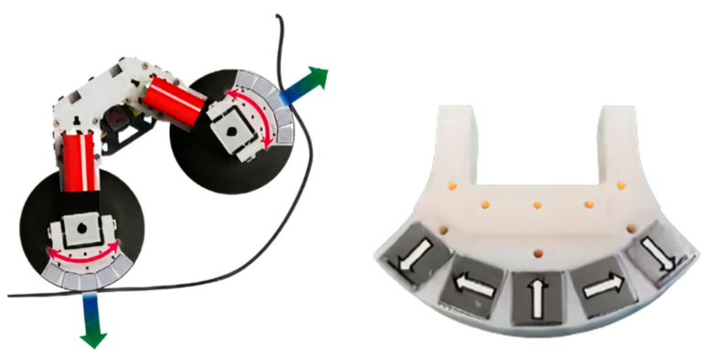
- To analyze existing magnetic wheel structures;
- To create a device capable of moving over high-situated above-ground gas pipelines and monitoring their technical condition;
- To test the device on a test rig comprising generic obstacles of typical gas pipeline;
- To make recommendations on the organization of work using the developed device.
2. Theoretical Study
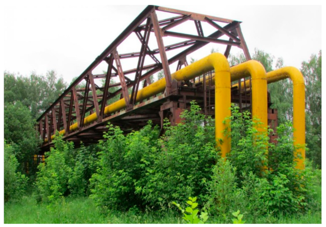
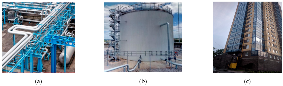
2.1. Analysis of Spatial Configurations of the Most Common Objects
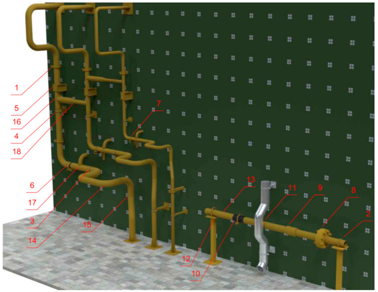
2.2. Development of an Experimental Test Rig
2.3. Review of the World Experience in Surveying Above-Ground Pipelines and Metal Structures of Complex Spatial Configuration
- Generally, drones have a low battery charge, therefore due to the presence of special inspection equipment the duration of the examination is about 15–20 min;
- As the battery capacity increases, the size of the drone and the number of screws grow, which negatively affects maneuverability;
- There is a high risk of accident while surveying narrow areas;
- It is not possible to inspect the complex pipe manifold due to advanced maneuvering.
- Limited on-board computer selection caused by weight restriction;
- High control complexity compared to land-based devices.
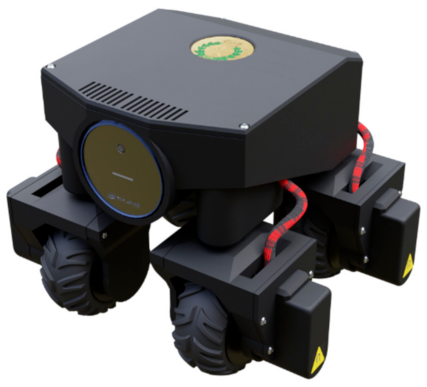
2.4. Design of Wireless Mobile Robot Crawler System for Pipe Inspection
- We have used the most suitable constructive materials that will ensure sufficient durability (Table 4);
- Maintainability is provided with the possibility of large-unit repair. In addition, the sensors are easily removable, this allows them to be «hot» replaced in the field. Individual elements (fasteners, gears) are made of unified standard sizes—this allows them to achieve good interchangeability;
- Overall metrics of reliability of the device are still difficult to assess, as there is no extensive field experience.
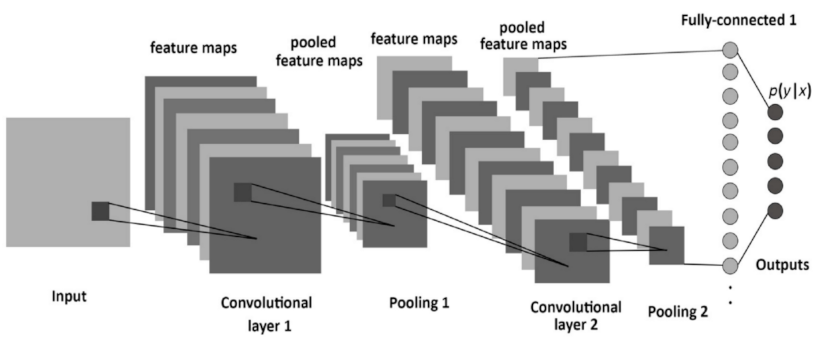
2.5. Neural Network Classification of Objects
- Axial displacement, change of the angle, rotations, other distortions;
- Fast staff turnover, the need for high data processing rate;
- A wide variety of different types of objects (elements of pipe manifold, supporting structures, defects, leaks);
- The use of high-resolution cameras results in a large amount of input data;
- Updating the database for the new survey.
- Decreased amount of learnable parameters and increased speed of learning in comparison with fully connected neural network [34];
- Ability to implement computations and network learning algorithms on graphic processors (GPU) [35];
- Displacement stability of input data [36];
- The use of convolutional kernels helps to avoid generalization of the displayed information. Scanning by parts allows to take into consideration a larger number of properties of the object, which improves the quality of recognition.
- Number of layers;
- Number of sites (neurons) in each layer;
- Type of activation function.
- Convolutional—performs convolution, which is characterized by the following parameters:
- Filters: number of output channels;
- Kernel size: convolutional kernel, is a local receptive field that specifies the width and height of the 2D convolution window;
- Padding: function that allows to create a zero-fill around the perimeter of the input image, so that the output has the same width and height;
- Activation: activation function;
- Input shape: dimension of the input signal.
- Pooling—this layer works in a similar way to the convolutional layer, but it does not have the convolutional kernel, but the pooling layer calculates the maximum or average values of the input data;
- Reshaping layers—change the dimension the input data;
- Dense—fully connected layer;
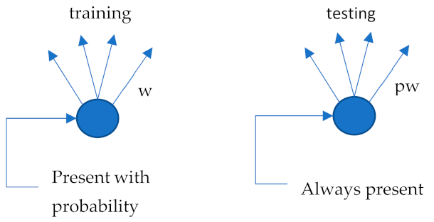
- Dropout—regularization technique that allows to avoid overfitting by keeping neurons in a state of activity (not zero) with a given probability.
- Fast in computation
- 1.
- Gradients do not disappear for ;
- 2.
- Provides fast convergence in practice;
- 3.
- Works if x < 0, which ensures continuous computing, as opposed to function ReLU ( [37].
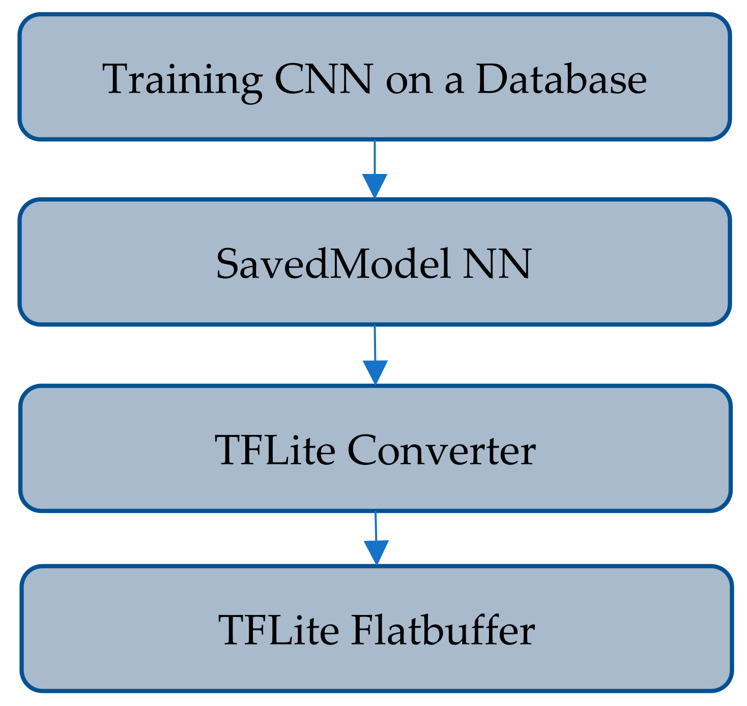
- Optimization for machine learning on the device, excluding 5 key constraints: delay (no return to server), confidentiality (no personal data leaving the device), connectivity (no Internet connection required), size (reduced model and binary size), and energy consumption (efficient output and lack of network connections, possibility to reduce the weight of the used computer in the robotic device) [43];
- Support for multiple platforms including Linux devices, microcontrollers, and microcomputers (if there is a need to overfit to a new data set, the process can be performed directly on a robotic device);
- High performance with hardware acceleration and model optimization.
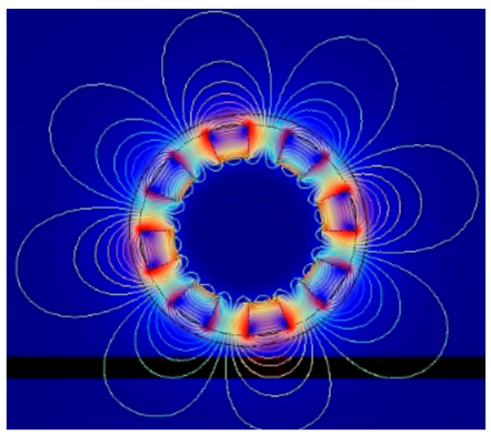
2.6. Modelling of Wheel Magnetic Fields
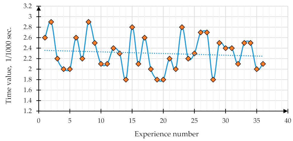
3. Experimental Apparatus and Procedure
Description of Experimental Device Survey
4. Results and Discussion
5. Conclusions
Author Contributions
Funding
Institutional Review Board Statement
Informed Consent Statement
Data Availability Statement
Acknowledgments
Conflicts of Interest
References
- Jose, J.; Devaraj, D.; Mathanagopal, R.M.; Ramanathan, K.C.; Tokhi, M.O.; Sattar, T.P. INVESTIGATIONS ON THE EFFECT OF WALL THICKNESS ON MAGNETIC ADHESION FOR WALL CLIMBING ROBOTS. Int. J. Robot. Autom. 2021, 36. [Google Scholar] [CrossRef]
- Trujillo, M.Á.; Martínez-de Dios, J.R.; Martín, C.; Viguria, A.; Ollero, A. Novel Aerial Manipulator for Accurate and Robust Industrial NDT Contact Inspection: A New Tool for the Oil and Gas Inspection Industry. Sensors 2019, 19, 1305. [Google Scholar] [CrossRef] [PubMed] [Green Version]
- Jimenez-Cano, A.E.; Braga, J.; Heredia, G.; Ollero, A. Aerial Manipulator for Structure Inspection by Contact from the Underside. In Proceedings of the 2015 IEEE/RSJ International Conference on Intelligent Robots and Systems (IROS), Hamburg, Germany, 28 September–2 October 2015; pp. 1879–1884. [Google Scholar]
- SAIR–Arabian Robotics Company. Available online: http://arabianbots.com/sair/ (accessed on 13 April 2022).
- Aкycтичecкиe Koнтpoльныe Cиcтeмы-Cкaнep-Дeφeктocкoп A2072 IntroScan. Available online: https://acsys.ru/skaner-defektoskop-a2072-introscan/ (accessed on 13 April 2022).
- Nguyen, S.; La, H. Development of a Steel Bridge Climbing Robot. In Proceedings of the 2019 IEEE/RSJ International Conference on Intelligent Robots and Systems (IROS), Macau, China, 3–8 November 2019. [Google Scholar] [CrossRef] [Green Version]
- Viktor BIKE–Inspection Robotics. Available online: https://inspection-robotics.com/bike/ (accessed on 13 April 2022).
- Wang, R.; Kawamura, Y. An Automated Sensing System for Steel Bridge Inspection Using GMR Sensor Array and Magnetic Wheels of Climbing Robot. J. Sens. 2016, 2016, 1–15. [Google Scholar] [CrossRef] [Green Version]
- Past Projects. Available online: https://www.isr.uc.pt/index.php/projects/past-projects?task=showprojects.show%28%29&idProject=13 (accessed on 13 April 2022).
- Burmeister, A.; Pezeshkian, N.; Talke, K.; Ostovari, S.; Everett, H.; Hart, A.; Gilbreath, G.; Nguyen, H. Design of a Multi-Segmented Magnetic Robot for Hull Inspection. In Proceedings of the ASNE Mega Rust 2014: Naval Corrosion Conference, San Diego, CA, USA, 24 June 2014. [Google Scholar]
- Trekker, D. DT340L Pipe Crawler Package. Available online: https://www.deeptrekker.com/shop/products/dt340l-pipe-crawler-package (accessed on 13 April 2022).
- Robot System: Magnet Crawler-Marine Inspection Robotic Assistant System. Available online: https://robotik.dfki-bremen.de/en/research/robot-systems/magnet-crawler/ (accessed on 13 April 2022).
- EMAT Thickness Measurement RobotRover Inspectioning Technology Co., Ltd. Available online: http://www.ritinspection.com/products/287.html (accessed on 13 April 2022).
- Tang, Y.; Song, H.; Yu, Y.; Zhang, J.; Hu, W.; Guo, X. Dynamic Simulation Analysis and Experiment of Large-Caliber Self-Propelled Pipeline Crawler Based on ADAMS. J. Phys. Conf. Ser. 2021, 2095, 012049. [Google Scholar] [CrossRef]
- Khan, M.; Chuthong, T.; Do, C.; Thor, M.; Billeschou, P.; Larsen, J.; Manoonpong, P. ICrawl: An Inchworm-Inspired Crawling Robot. IEEE Access 2020, 8, 1. [Google Scholar] [CrossRef]
- Magnetic Drive Wheel for Wall Climbing Robot-Faizeal. Available online: https://www.fzmag.com/magnetic-drive-wheel-for-wall-climbing-robot/ (accessed on 13 April 2022).
- Zhang, Y.; Dai, Z.; Xu, Y.; Qian, R. Design and Adsorption Force Optimization Analysis of TOFD-Based Weld Inspection Robot. J. Phys. Conf. Ser. 2019, 1303, 012022. [Google Scholar] [CrossRef]
- Mahmood, S.; Bakhy, S.; Tawfik, M. Magnetic–Type Climbing Wheeled Mobile Robot for Engineering Education. IOP Conf. Ser. Mater. Sci. Eng. 2020, 928, 022145. [Google Scholar] [CrossRef]
- Lawrence, K.H. Design of Permanent Multipole Magnets with Oriented Rare Earth Cobalt Materials. Nucl. Instrum. Methods 1980, 169, 1–10. [Google Scholar]
- Bjørk, R.; Bahl, C.; Smith, A.; Pryds, N. Optimization and Improvement of Halbach Cylinder Design. J. Appl. Phys. 2008, 104, 013910. [Google Scholar] [CrossRef] [Green Version]
- Zhang, M.; Zhang, X.; Li, M.; Cao, J.; Huang, Z. Optimization Design and Flexible Detection Method of a Surface Adaptation Wall-Climbing Robot with Multisensor Integration for Petrochemical Tanks. Sensors 2020, 20, 6651. [Google Scholar] [CrossRef] [PubMed]
- Eto, H.; Asada, H. Development of a Wheeled Wall-Climbing Robot with a Shape-Adaptive Magnetic Adhesion Mechanism. In Proceedings of the 2020 IEEE International Conference on Robotics and Automation (ICRA), Paris, France, 31 May–31 August 2020. [Google Scholar] [CrossRef]
- Intel® RealSenseTM LiDAR Camera L515. Available online: https://www.intelrealsense.com/lidar-camera-l515/ (accessed on 13 April 2022).
- Yang, P.; Bai, H.; Xue, X.; Xiao, K.; Zhao, X. Vibration Reliability Characterization and Damping Capability of Annular Periodic Metal Rubber in the Non-Molding Direction. Mech. Syst. Signal Process. 2019, 132, 622–639. [Google Scholar] [CrossRef]
- Shen, G.; Li, M.; Xue, X. Damping Energy Dissipation and Parameter Identification of the Bellows Structure Covered with Elastic-Porous Metal Rubber. Shock Vib. 2021, 2021, 1–12. [Google Scholar] [CrossRef]
- Xue, X.; Ruan, S.; Li, A.; Bai, H.; Xiao, K. Nonlinear Dynamic Modelling of Two-Point and Symmetrically Supported Pipeline Brackets with Elastic-Porous Metal Rubber Damper. Symmetry 2019, 11, 1479. [Google Scholar] [CrossRef] [Green Version]
- Mumtaz, M.; Mansoor, A.; Masood, H. A New Approach to Aircraft Surface Inspection Based on Directional Energies of Texture. In Proceedings of the 2010 20th International Conference on Pattern Recognition, Istanbul, Turkey, 23–26 August 2010; pp. 4404–4407. [Google Scholar]
- Jahanshahi, M.; Masri, S. Effect of Color Space, Color Channels, and Sub-Image Block Size on the Performance of Wavelet-Based Texture Analysis Algorithms: An Application to Corrosion Detection on Steel Structures. In Proceedings of the Computing in Civil Engineering (2013), Los Angeles, CA, USA, 24 June 2013; pp. 685–692. [Google Scholar]
- Ji, G.; Zhu, Y.; Zhang, Y. The Corroded Defect Rating System of Coating Material Based on Computer Vision. In Transactions on Edutainment VIII; Springer: Berlin/Heidelberg, Germany, 2012; Volume 7220, pp. 210–220. [Google Scholar]
- Siegel, M.; Gunatilake, P.; Podnar, G. Robotic Assistants for Aircraft Inspectors. Instrum. Meas. Mag. IEEE 1998, 1, 16–30. [Google Scholar] [CrossRef]
- Bahaa, B.; Zaidan, A.; Alanazi, H.; Rami, A. Towards Corrosion Detection System. Int. J. Comput. Sci. Issues 2010, 7. [Google Scholar]
- Ortiz, A.; Bonnin-Pascual, F.; Garcia-Fidalgo, E.; Company-Corcoles, J. Vision-Based Corrosion Detection Assisted by a Micro-Aerial Vehicle in a Vessel Inspection Application. Sensors 2016, 16, 2118. [Google Scholar] [CrossRef] [PubMed]
- Lin, T.-Y.; Dollár, P.; Girshick, R.B.; He, K.; Hariharan, B.; Belongie, S.J. Feature Pyramid Networks for Object Detection. In Proceedings of the IEEE Conference on Computer Vision and Pattern Recognition (CVPR), Honolulu, HI, USA, 21–26 July 2017. [Google Scholar] [CrossRef] [Green Version]
- Albawi, S.; Abed Mohammed, T.; ALZAWI, S. Understanding of a Convolutional Neural Network. In Proceedings of the 2017 International Conference on Engineering and Technology (ICET), Antalya, Turkey, 21–23 August 2017. [Google Scholar]
- Luo, Z.; Liu, H.; Wu, X. Artificial Neural Network Computation on Graphic Process Unit. In Proceedings of the 2005 IEEE International Joint Conference on Neural Networks, Montreal, QC, Canada, 31 July–4 August 2005; Volume 1, pp. 622–626. [Google Scholar]
- Sultana, F.; Sufian, A.; Dutta, P. Advancements in Image Classification Using Convolutional Neural Network|Request PDF. In Proceedings of the 2018 Fourth International Conference on Research in Computational Intelligence and Communication Networks (ICRCICN), Kolkata, India, 22–23 November 2018. [Google Scholar]
- Nwankpa, C.; Ijomah, W.; Gachagan, A.; Marshall, S. Activation Functions: Comparison of Trends in Practice and Research for Deep Learning. arXiv 2018, arXiv:1811.03378. [Google Scholar]
- Ghosh, A.; Sufian, A.; Sultana, F.; Chakrabarti, A.; De, D. Fundamental Concepts of Convolutional Neural Network. In Recent Trends and Advances in Artificial Intelligence and Internet of Things; Springer: Cham, Switzerland, 2020; pp. 519–567. ISBN 978-3-030-32643-2. [Google Scholar]
- Шaклa, Hишaнт-Maшиннoe Oбyчeниe & TensorFlow [Teкcт]: [16+]-Search RSL. Available online: https://search.rsl.ru/ru/record/01009872794? (accessed on 13 April 2022).
- Gafarov, F.; Galimyanov, A. Artificial Neural Networks and Their Applications, 1st ed.; Kazan University: Kazan, Russia, 2018; pp. 25–28. [Google Scholar]
- TeнзopΦлoy Лaйт|TensorFlow Lite. Available online: https://www.tensorflow.org/lite/guide?hl=ru (accessed on 13 April 2022).
- FlatBuffers: FlatBuffers. Available online: https://google.github.io/flatbuffers/ (accessed on 13 April 2022).
- Cпpaвoчник пo API TensorFlow Lite. Available online: https://www.tensorflow.org/lite/api_docs?hl=ru (accessed on 13 April 2022).


| Pipe Supports | ||
|---|---|---|
| Schematic Item | Visual Representation | Short Title |
| 1 |  | A variety of options for fixing pipelines to building walls and metal structures |
| 2 |  | |
| 3 |  | |
| 4 |  | |
| 5 |  | |
| 6 |  | |
| 7 |  | |
| Specific types of obstacles | ||
| Schematic item | Visual representation | Short title |
| 8 |  | Insulating flanged joint |
| 9 |  | Insulating monolithic sleeve |
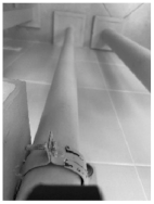
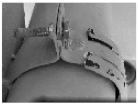
| 10 |  | Support with U-bolt clamp and rubber insert |
| 11 |  | Test site of bypass with rainwater pipes |
| 12 |  | Not sealed tightly on the saddle clamp |
| 13 |  | Faulty welded joint |
| Fittings | ||
| Schematic item | Visual representation | Short title |
| 14 |  | Bend 90° |
| 15 |  | Bend 45° |
| 16 |  | Straight T-junction |
| 17 |  | Transition T-junction |
| 18 |  | Concentric reducer |
| Parameter | Unit of Measure | Saudi Aramco [4] | INTROSCAN [5] | ARA Lab [6] | Waygate Technologies [7] | University of Tsukuba [8] | University of Coimbra [9] | SSC Pacific [10] | DEEP TREKKER [11] | DFKI [12] | RIT [13] |
|---|---|---|---|---|---|---|---|---|---|---|---|
| Dimensions: | |||||||||||
| −length −width −height | mm | 325 180 215 | 400 270 240 | 163 145 198 | 247 190 217 | 345 210 130 | 240 240 140 | No information | 710 406 228 | 380 280 150 | 380 130 120 |
| Weight | kg | 9.5 | 18 | 3 | 9.6 | 2.3 | 1.12 | No information | 16.6 | 0.67 | 6 |
| Maximum speed | mm/s | 140 | 83,3 | 200 | 50 | 320 | 140 | No information | 200 | 500 | No information |
| Gas detector | – | CH4, CO2, O2 | Absent | Absent | Absent | Absent | Absent | Absent | Absent | Absent | Absent |
| Type of sensor | – | Ultrasonic dry contact | Ultrasonic dry contact | Infrared sensor and eddy current sensor | Ultrasonic wet contact | Hall transducer | Absent | Absent | Absent | Absent | Ultrasonic dry contact |
| Camera | pcs | 1 | 1 | 2 | 2 | 0 | 0 | 1 | 1 | 1 | 2 |
| Operating temperature | °C | 0… +50 | −20… +60 | No information | No information | No information | No information | No information | 5… +40 | No information | 10… +50 |
| Obstacle negotiation | – | No | No | Partly | Partly | Partly | No | Yes | Partly | Partly | No |
| General view | – |  |  |  |  |  |  |  |  |  |  |
| LiDAR Intel RealSense L515 Parameters | |
|---|---|
| Type of tracking | Laser scanning |
| Operating range | 0.25–9 m |
| Depth camera resolution and FPS | 1024 × 768; 30 FPS |
| RGB camera resolution and FPS | 1920 × 1080; 30 FPS |
| Color depth camera resolution and FPS | 1920 × 1080; 30 FPS |
| Depth accuracy | 5 mm |
| Depth camera coverage | 70 × 55 degrees |
| RGB camera coverage | 70 × 43 degrees |
| Color depth camera coverage | 69 × 42 degrees |
| IMU sensor model | Bosch BMI085 |
| IMU sensor number of degrees of freedom | 6 |
| Speed of accelerometer data output | 100 Hz/200 Hz/400 Hz |
| Speed of gyroscope data output | 100 Hz/200 Hz/400 Hz |
| Operating temperature range of the environment | −20…+70 °C |
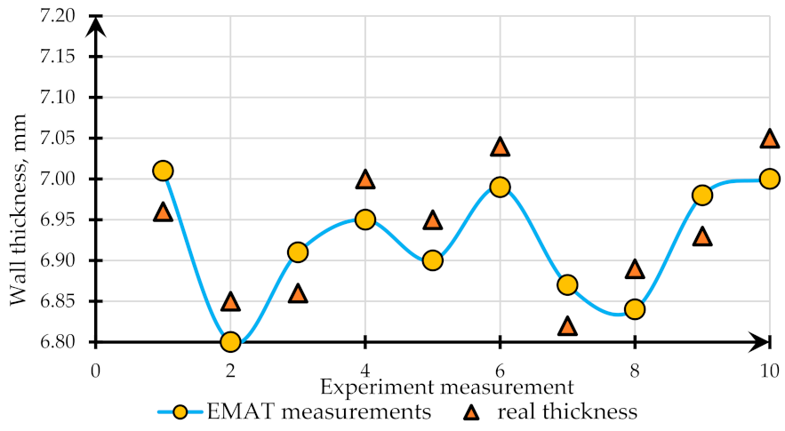
| EMAT parameters | |
| Range of thickness measured for steel | 2–80 mm |
| Thickness measurement uncertainty | 0.08 mm |
| Permissible gap between sensor and unit under test | up to 4 mm |
| Permissible misalignment of sensor relatively to surface normal | ±25 degrees |
| Minimum permissible radius of surface curvature | ≥10 mm |
| Device operating frequency | 4 MHz |
| Operating temperature range of the testing object surface | −20…+80 °C |
| Robot crawler parameters | |
| Width | 180 mm |
| Length | 180 mm |
| Height | 165 mm |
| Mass (without accumulator) | 1.8 kg |
| Kinematics | 4WD, fully rotatable |
| № | Constructive Part | Material | Durability |
|---|---|---|---|
| 1 | Spur gear | Nylon | 5 years |
| 2 | Body | ABS | up to 10 years |
| 3 | Wheel tire | Polyurethane | 5 years |
| 4 | Wheel shaft | Titanium | 30 years |
| CNN for Obstacle Identification | CNN for Detecting Complication Signatures | ||||
|---|---|---|---|---|---|
| Layer (Type) | Output Shape | Number of Parameters | Layer (Type) | Output Shape | Number of Parameters |
| Input | 250 × 250 × 1 | 0 | Input | 250 × 250 × 3 | 0 |
| Convolutional | 250 × 250 × 128 | 1280 | Convolutional | 250 × 250 × 16 | 448 |
| Convolutional | 250 × 250 × 128 | 147,584 | |||
| MaxPooling | 125 × 125 × 128 | 0 | Convolutional | 250 × 250 × 16 | 4640 |
| Dropout | 125 × 125 × 128 | 0 | |||
| Convolutional | 125 × 125 × 128 | 147,584 | MaxPooling | 125 × 125 × 32 | 0 |
| Convolutional | 125 × 125 × 128 | 147,584 | |||
| MaxPooling | 62 × 62 × 128 | 0 | Dropout | 125 × 125 × 32 | 0 |
| Dropout | 62 × 62 × 128 | 0 | |||
| Convolutional | 62 × 62 × 128 | 147,584 | Convolutional | 125 × 125 × 32 | 9248 |
| Convolutional | 62 × 62 × 128 | 147,584 | |||
| MaxPooling | 31 × 31 × 128 | 0 | Convolutional | 125 × 125 × 32 | 18,496 |
| Dropout | 31 × 31 × 128 | 0 | |||
| Convolutional | 31 × 31 × 128 | 147,584 | MaxPooling | 62 × 62 × 64 | 0 |
| Convolutional | 31 × 31 × 128 | 147,584 | |||
| MaxPooling | 15 × 15 × 128 | 0 | Dropout | 62 × 62 × 64 | 0 |
| Dropout | 15 × 15 × 128 | 0 | |||
| Flatten | 28,800 | 0 | Flatten | 246,016 | 0 |
| Dense | 128 | 3,686,528 | Dense | 256 | 6,2980,352 |
| Dropout | 128 | 0 | Dropout | 256 | 0 |
| Dense | 11 | 1419 | Dense | 2 | 514 |
| Total parameters: | 4,722,315 | Total parameters: | 63,013,698 | ||
| Model | PCE-FM200 |
|---|---|
| General view of device |  |
| Measurement range | 0…20 kg/0…200 N |
| Resolution | 0,05 kg/0,2 N |
| Accuracy | ±0.5% |
| Unit | gram/newton |
| Extreme overload | 50% (max. up to 150 kg) |
| Metering function | Measurement of compression and tensile forces |
| № | Image Id | Image Array | Processed Image Array | Object Id | Object Name | Object Array | Bbox xmin | Bbox ymin | Bbox ymax | Bbox xmax |
|---|---|---|---|---|---|---|---|---|---|---|
| 0 | 0.0 | [[202, 200, 200, 206, 205, 207, 204, 204, 200, …]] | [[202, 200, 200, 206, 205, 207, 204, 204, 200, …]] | 0.0 | Insulating flanged joint | [[[255, 255, 255, 255, 255, 255, 255, 255, 255, …]]] | 84.0 | 25.0 | 225.0 | 265.0 |
| 1 | 0.0 | [[202, 200, 200, 206, 205, 207, 204, 204, 200, …]] | [[223, 230, 229, 218, 222, 221, 214, 213, 212, …]] | 1.0 | Support with U-bolt clamp and rubber insert | [[[255, 255, 255, 255, 255, 255, 255, 255, 255, …]]] | 243.0 | 3.0 | 250.0 | 336.0 |
| 2 | 1.0 | [[208, 202, 202, 199, 199, 202, 199, 198, 200, …]] | [[208, 202, 202, 199, 199, 202, 199, 198, 200, …]] | 2.0 | Pipe clamp | [[[255, 255, 255, 255, 255, 255, 255, 255, 255, …]] | 215.0 | 97.0 | 227.0 | 313.0 |
| … | … | … | … | … | … | … | … | … | … | … |
| 936 | 846.0 | [[68, 70, 69, 68, 69, 68, 65, 63, 62, 62, 62, …]] | [[68, 70, 69, 68, 69, 68, 65, 63, 62, 62, 62, …]] | 936.0 | Bend 90° | [[[255, 255, 255, 255, 255, 255, 255, 255, 255, …]]] | 5.0 | 4.0 | 252.0 | 321.0 |
| Input Data | Initial Processing (Data Dimension Change) | Output Data After CNN Processing on Obstacle Element Detection and Classification | Isolated Data of Discovered Object |
|---|---|---|---|
 |  |  |  |
Publisher’s Note: MDPI stays neutral with regard to jurisdictional claims in published maps and institutional affiliations. |
© 2022 by the authors. Licensee MDPI, Basel, Switzerland. This article is an open access article distributed under the terms and conditions of the Creative Commons Attribution (CC BY) license (https://creativecommons.org/licenses/by/4.0/).
Share and Cite
Pshenin, V.; Liagova, A.; Razin, A.; Skorobogatov, A.; Komarovsky, M. Robot Crawler for Surveying Pipelines and Metal Structures of Complex Spatial Configuration. Infrastructures 2022, 7, 75. https://doi.org/10.3390/infrastructures7060075
Pshenin V, Liagova A, Razin A, Skorobogatov A, Komarovsky M. Robot Crawler for Surveying Pipelines and Metal Structures of Complex Spatial Configuration. Infrastructures. 2022; 7(6):75. https://doi.org/10.3390/infrastructures7060075
Chicago/Turabian StylePshenin, Vladimir, Anastasia Liagova, Alexander Razin, Alexander Skorobogatov, and Maxim Komarovsky. 2022. "Robot Crawler for Surveying Pipelines and Metal Structures of Complex Spatial Configuration" Infrastructures 7, no. 6: 75. https://doi.org/10.3390/infrastructures7060075
APA StylePshenin, V., Liagova, A., Razin, A., Skorobogatov, A., & Komarovsky, M. (2022). Robot Crawler for Surveying Pipelines and Metal Structures of Complex Spatial Configuration. Infrastructures, 7(6), 75. https://doi.org/10.3390/infrastructures7060075