Abstract
As more and more container terminals are becoming intelligent, different kinds of sensors are widely installed at different locations of the cranes and collect a large amount of data. In order to effectively utilize and manage these huge amounts of actual working data of different sensors and grasp the status of the terminal, this article proposes a data processing framework that integrates the crane load, energy consumption, crane trolley speed and crane gearbox vibration signals of the container terminal. Firstly, the load spectrum of the crane load is calculated by the non-parametric density estimation method in probabilistic statistics and the energy consumption curves are obtained. Secondly, the driving cycle of the crane trolley speed are constructed by drawing on the method in the transportation field. Finally, the vibration signals of the crane gearbox are used for anomaly detection by unsupervised methods; at the same time, clustering results can also be used as the basis for extracting typical vibration signals and removing redundant data.
1. Introduction
With the development of IoT (Internet of Things) and big data technologies, container terminals are evolving from the traditional operation mode that requires a lot of human involvement to intelligent and automated ports [1].
In recent years, many ports in China have completed the renovation and construction of automation one after another, such as the Haitian Terminal in Xiamen, the fully automated terminal in Qingdao, the automated Yangshan Deepwater Port, the Nansha Port in Guangzhou and so on. During this automation process, different kinds of sensors are widely installed on various parts of the cranes and they can collect digital signals in gigabytes every day.
Meanwhile, many areas of research in automated container terminals are still at a preliminary stage, especially the application and analysis of big data technology [2]. There are many studies on port scheduling optimization and crane operation optimization [3,4], but they usually implement the application after the information is collected from scratch, and there is little practice when the magnitude of the data reaches a high level. Therefore, how to help smart harbor managers to process and analyze these mass data collected from practical projects and apply the results to the actual project is an urgent problem at this stage. Moreover, many aspects of port operations can be improved with the help of data.
The health status of cranes in ports is one of the key indicators of great concern. The load spectrum is one of the important bases for predicting the equipment life, and how to estimate the load spectrum from the available data of the port is a problem that needs to be studied. Geng et al. [5] used the hybrid distribution probability model to construct the road load spectrum of the test site, and then estimated the parameters of the Pareto distribution using the maximum likelihood, and finally got the load spectrum of one and two dimensions. Luo et al. [6] established the load spectrum of a train axle by processing the load spectrum and fitting its mean value and the amplitude. Zhang et al. [7] proposed a facility maintenance strategy based on a randomized structural deterioration model for port infrastructures, and the results showed an improved level of understanding of the structural health of the port by managers.
The working cycle time of a crane is variable. The shorter the time of each working cycle, the greater the handling capacity of the crane and the higher the handling efficiency. This will directly affect the berth allocation of the terminal and ultimately affect the efficiency of the terminal [8]. In order to describe the driving state of a vehicle, it is usually necessary to obtain a series of velocity-time values to construct the driving cycle of the vehicle. For the crane, the object is the trolley on the crane. The method in the problem of the vehicle working cycle can be used for reference in the research of cranes, which requires multi-step preprocessing, eigenvalue calculation and data analysis [9]. Among them, data analysis methods usually use the k-means [10] method to analyze their eigenvalues and Markov chain [11,12] to construct a typical working cycle.
In order to guarantee the normal working of the mechanism, the key component of the mechanism, i.e., the gearbox, needs to be monitored in real time. The vibration signals of the gearbox can be obtained through the acceleration sensors installed at different locations of the gearbox. How to reflect the current state of the equipment through these signals is also a problem that needs to be studied. Wang et al. [13] used an improved feature selection technique in the condition monitoring of planetary gearboxes with an unsupervised clustering algorithm for fault diagnosis. The method is tested when there are cracks in the sun gear, the planet gear and the gear ring. The results show that the method is effective. Aiming at the nonlinearity of the gearbox vibration signal, Zhang et al. [14] used MFDFA to calculate the characteristic value of the gearbox as the application object of the improved k-means method; it achieved better results in the gearbox fault experiment.
In addition, energy and environmental issues have been hot topics recently. As a hub connecting the sea and land, the terminal consumes a lot of energy to transship bulk cargo, which will lead to high energy costs and accompanying high pollution and greenhouse gas emissions [15]. Port operators are also looking to reduce energy consumption by applying various strategies, such as energy-aware optimization of operations [16] and peak shaving [17]. These studies propose a variety of berth allocation and quay crane assignment strategies to reduce power consumption or reduce grid burden. Iris et al. [18] studied optimal operations plan, demand response and optimal power flow from the perspective of port microgrid. The results prove that the energy cost can be reduced under the action of the energy storage system and the demand response mechanism.
As can be seen, there are some new technologies that can be applied to the port to improve the intelligence. However, they do not solve the new problems brought about by the increase in the level of data in smart harbors. A smart harbor can collect very similar data in gigabytes every day. How does one process these data to obtain information from them? How does one delete similar data to reduce the storage space burden? In order to solve the challenges brought about by massive data and obtain valuable information at the same time, this article proposes a framework for the application of big data technology in ports. Under this framework, the load spectrum, energy consumption, typical working cycle for trolley and vibration signal clustering of the gearbox are obtained. The results will be used to help port operators gain insight into the port operations and equipment health and find typical data within a specified period, providing a basis for removing duplicate similar data.
2. Problem and Solution
Most of the cranes in container terminals are quay container cranes, as shown in Figure 1. These cranes are approximately 110 m long, 30 m wide and 70 m high, weighing up to 580 tons and capable of gripping containers of up to 60 tons. Manual inspection of such a large structure involves a lot of labor. Therefore, the monitoring of these large steel structures is of great importance.
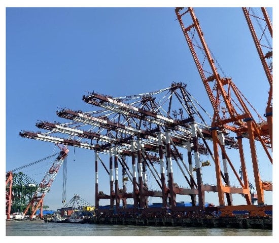
Figure 1.
Quay Container Cranes.
As mentioned above, the new smart port has achieved multi-channel monitoring of cranes, as shown in Figure 2. The main monitoring object of the container terminal is the ship-to-shore quay crane. Various sensors can monitor the crane lifting load, the crane trolley running speed/direction, the vibration signal of the key mechanism of gear box and so on.
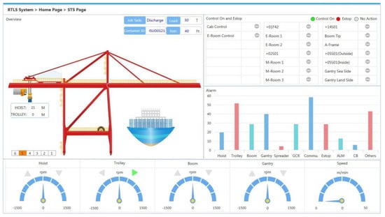
Figure 2.
Crane Monitoring Interface.
For port operators, the infrastructure for data monitoring is gradually improving, but there is still a big gap in how data are applied. In addition, the growing amount of monitoring data is also a problem that has to be faced.
For the crane lifting load, lifting position, trolley speed and vibration signal of the gearbox collected at the port, this article proposes a data mining framework, as shown in Figure 3. The specific methods are: firstly, the crane load spectrum is obtained by statistically estimating the crane lifting load through a non-parametric kernel density estimation algorithm and the power under different loads can also be calculated; secondly, by drawing on the typical driving cycle construction problem in the transportation field, the eigenvalues of the trolley speed on the crane are calculated, and the typical working cycle is obtained through the k-means algorithm; finally, for the vibration signal of the gearbox, its time-domain and frequency-domain eigenvalues are calculated, and the k-means algorithm is used for unsupervised fault diagnosis of the gearbox; its clustering center can also represent the vibration data over a period of time and be retained as typical data for a long time.
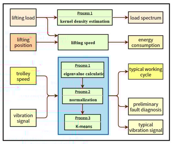
Figure 3.
Data Mining Framework.
3. Methods
3.1. Kernel Density Estimation of the Load Spectrum
In probability statistics, it is necessary to analyze the collected data to solve its underlying probability density. The method used is usually parametric method or non-parametric method. The parameter method needs to assume that the sample data conforms to a distribution law, and then solve the parameters in this distribution law [19]. The non-parametric method does not require the assumption of a specific form of the distribution function, and the probability density estimation results are determined by the data itself [20]. For the load spectrum of the crane, because the weight of the transported cargo is unknown and completely random, the spectrum may have multiple peaks and may change with time. This makes it infeasible to use a preset probability distribution for estimation, whereas kernel density estimation does not need to preset a probability distribution and can achieve better results. As a result, the non-parametric method of kernel density estimation is chosen to calculate the load spectrum of the crane lifting weight.
The kernel density (also called Parzen window) estimation algorithm, which is an extension of the idea of Gaussian mixture model, generates a set of probability density functions for all sample points to obtain an approximate target probability distribution. The one-dimensional kernel density can be calculated as follows:
where is the sample capacity, is the bandwidth and is the kernel function. The kernel function is a probability density function, which needs to satisfy the condition that the value is non-negative and the integration is one. The kernel function and bandwidth determine the accuracy and smoothness of the final estimated density. Commonly used kernel functions are square window function, trigonometric window function, Gaussian function, etc. In this article, Gaussian function is used as the kernel function.
3.2. Preprocessing of Trolley Speed Signals
The speed signal is obtained by a sensor mounted on the coupling between the gearbox and the motor of the trolley mechanism and is able to reflect the fluctuation of the trolley motor speed over a period of time. A simple analysis of the speed data shows that there are obvious skipping phenomena in the signal collected on site, and the signal jitter is strong, shown in Figure 4, which will create obstacles for the subsequent analysis and calculation. Therefore, the speed signal needs to be preprocessed.
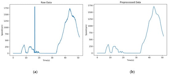
Figure 4.
Comparison before and after speed preprocessing: (a) Raw Data, and (b) Preprocessed Data.
First, by calculating the speed difference between adjacent moments, we can obtain the real-time angular acceleration of the crane motor shaft. Points with angular acceleration greater than a threshold are marked as abnormal. Secondly, by calculating the mean value of other normal data near the anomaly point, the corrected data can be obtained.
In addition, the signal usually still contains a certain amount of noise, and the Savitzky–Golay filter based on the least squares fitting theory can effectively reduce the influence of the mutation point [21]. For a time-series data point x(t), if there are M units of data before and after the moment , use these 2M + 1 units of data for fitting:
where N is the order of the polynomial and 2M + 1 is the window width.
The minimum mean square error of the fit is:
Letting the partial derivative of this error with respect to be zero, each value of can be calculated.
The data at the moment t0 can eventually be solved for as follows:
where can be obtained from the set of equations solved for .
The original rotational speed data and the data after outlier processing and data smoothing are shown in Figure 4.
3.3. The Characteristic Value of Trolley Speed
In order to characterize the driving cycle of the trolley and to analyze the characteristics quantitatively, it is necessary to calculate the characteristic parameters as its reference basis [22]. In this article, 13 characteristic values are selected to describe the trolley speed: average speed, average travel speed, average acceleration, average deceleration, idle time ratio, acceleration time ratio, deceleration time ratio, speed standard deviation, acceleration standard deviation, running time, maximum acceleration, minimum deceleration and maximum speed [12].
Because the speed data in this article is segmented time series, each time series is a crane operation process. There is no need for additional segmentation of the signal segments, and the feature values can be calculated directly. After the eigenvalues are calculated for all segments, the eigenvalues need to be normalized in order to prevent the difference influence ratio of the eigenvalues in the subsequent processing due to the difference of the order of magnitude. In this article, the normalization method of Z-Score is used to normalize the feature matrix by the following equation.
where is the mean of all sample data and is the standard deviation of all sample data.
The matrix of eigenvalues after normalization is shown in Table 1.

Table 1.
The eigenvalues matrix of trolley speed.
3.4. Vibration Signal Eigenvalue Calculation
In practice, the collected vibration signal is a segment of random discrete signal, and in order to reflect the vibration pattern of the segment, the statistical eigenvalues of the segment are used as the eigenvalues to characterize the signal [23]. The statistical eigenvalues of the vibration signal can be divided into two categories: time domain statistical eigenvalues and frequency domain statistical eigenvalues [24]. The calculation formula is shown in Table 2.
Table 2.
Time domain eigenvalue.
The time domain statistical characteristic values used in this article include mean, standard deviation, root mean square (RMS), peak indicator, pulse indicator, waveform indicator, kurtosis indicator, skewness indicator, margin indicator and root-mean-square amplitude. The standard deviation reflects the degree of fluctuation of the signal around the mean value; the root-mean-square value describes the energy of the vibration signal, which has a good stability and repeatability; the peak indicator and pulse indicator can be used to detect whether there is shock in the signal; the kurtosis indicator is sensitive to the shock characteristics of the signal, and when the value is too large, it indicates that there may be shock vibration in the machinery due to excessive clearance, the existence of the broken slide joint surface, etc.; the margin indicator can be used to detect the wear of mechanical equipment; the skewness indicator reflects the asymmetry of the vibration signal; the root-mean-square amplitude is not only a reflection of the mean value of the signal vibration but also of the fluctuation and dispersion of the signal.
Frequency domain statistical features include power spectrum center of gravity indicator, mean square spectrum, power spectrum variance, correlation factor, harmonic factor, origin moment of spectrum, etc. The power spectrum is a reflection of the variation of signal power with frequency in a unit frequency band, that is, the distribution of signal power in the frequency domain. Power is defined as the time-averaged component of the square of the amplitude, and this calculation can also be seen as the process of removing the phase information of the harmonic components in the frequency domain. The gravity center of power spectrum reflects the degree of change in energy center, which can better describe the changes in the frequency domain characteristics of the signal; the power spectrum variance reflects the degree of dispersion of the energy distribution; the power spectrum mean square frequency characterizes the location of the main band of the power spectrum; the correlation factor reflects the degree of correlation of the spectrum energy distribution; the harmonic factor reflects the distribution state and the spectral width of the spectrum; the origin moment of spectrum reflects the overall energy situation of the power spectrum. The calculation formula is shown in Table 3.
Table 3.
Frequency domain eigenvalue.
These time and frequency domain eigenvalues can better reflect the difference between mechanical equipment in fault and non-fault states, and the characteristic matrix is chosen as the object of machine learning. Again, these feature values need to be normalized to obtain better results.
3.5. Eigenvalue Dimensionality Reduction
For each vibration signal, a total of 16 eigenvalues can be calculated. Therefore, the dimension of the eigenvalue matrix will be n*16, where n is the number of vibration signal. For one signal, a 1*16 eigenvalue vector can be obtained. However, there may be information overlap among the feature values, in order to improve the efficiency of machine learning and reduce unnecessary computation; it is necessary to reduce the dimensionality of the feature values. In this article, principal component analysis (PCA) is used to reduce the dimensionality of the eigenvalue matrix. It performs orthogonal transformation on the values of related variables, thereby projecting them into the values of a series of linearly uncorrelated variables [25]. These uncorrelated variables are called principal components. These principal components will no longer have any physical meaning but represent deeper, uncorrelated intrinsic features of those former values.
Solving the covariance matrix of the normalized feature matrix, and then finding the eigenvalues of its covariance matrix, we can obtain the contribution rate of each component. The contribution rate indicates the ability of the principal components to represent the original data, and the larger the contribution rate is, the stronger the ability to comprehend the original variable data.
The contribution rate is defined as follows:
where λ is the eigenvalue of each component. Therefore, the number of components to be retained can be obtained after determining the value of CL, and the sum of contribution rates is generally required to be not less than 85%. In this article, the sum of contribution rate of vibration signal is 90.15% when 3 dimensions are retained after dimensionality reduction, which meets the requirement.
The vibration signal after normalization and dimensionality reduction is shown in Table 4.
Table 4.
Vibration eigenvalues after dimensionality reduction.
3.6. K-Means
The k-means algorithm [26] is a vectorized computational method that initially came from signal processing and is more commonly used as a clustering algorithm in many fields [27]. Because abnormal data and normal data have different eigenvalues, they will be distributed in different locations in the feature space, so the abnormal data can be separated by clustering algorithm. In addition, the distance in the feature space can reflect the similarity between data, so the center of each cluster can be used as the typical data representing the class. The k-means algorithm can specify the number of clusters, which will also facilitate the generation of a specified number of typical data. In this article, the method will be applied several times for the purpose of mining information from port data.
The essence of the k-means algorithm is to divide the sample points observed at one time into k clusters and to ensure that each sample point belongs to the cluster corresponding to its nearest cluster center.
The steps of k-means clustering are as follows:
In the first step, k clustering centers are selected, which are also called the mass center of the class. If the mass center is selected completely randomly, it may make the clustering process too computationally intensive and increase the number of unnecessary iterative steps. Therefore, it is necessary to increase the probability of selecting points that are far from the selected center of mass when selecting a new center of mass.
In the second step, for each sample point , the category to which it belongs is calculated with the following formula:
where is the sample, is the mass center of the class, is the new class to which the sample belongs and is the Euclidean distance between the two computations.
This step can be specifically divided into two steps: calculating the distance and finding new classes, and the main computational effort occurs in the distance calculation. To speed up the iterative clustering process, a large number of computational steps can be reduced by using the geometric properties of triangles through the Elkan algorithm.
In the third step, for each category, the position of its center of mass is recalculated according to the following equation.
Repeat the second and third steps until convergence or until the termination condition is reached.
The loss function is:
4. Results
4.1. Data set
In this article, an experiment based on real data was conducted, and the data are all collected from the actual working cycles of a container terminal in China, as shown in Figure 5 and Figure 6.
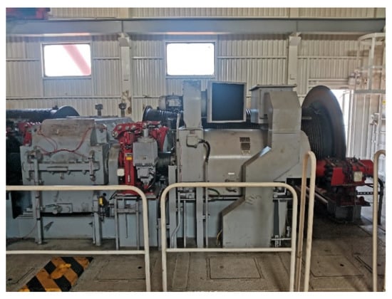
Figure 5.
The target mechanism to be monitored.
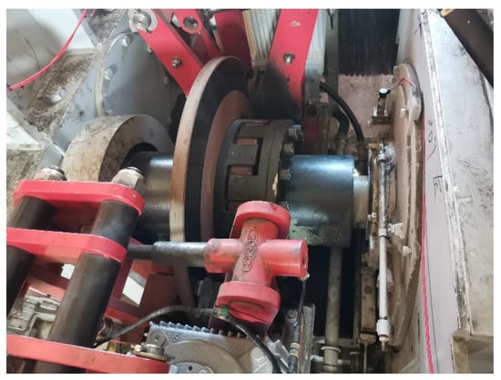
Figure 6.
The mounted sensor.
Each group of data records a complete working cycle of a crane, including hoisting mechanism lifting, trolley mechanism operation and hoisting mechanism lowering. The specific contents of each group of data include the signals of 16 vibration sensors, the signals of 2 speed sensors and the trolley position, lifting sling position and lifting weight obtained from the PLC (Programmable Logic Controller). These data are stored in csv format, and each group of data may contain multiple work cycles. In the preprocessing stage of the data, it is split into individual work cycles using the spreader unlock signal as a boundary. The sampling frequency of most signals is 1Hz, and the sampling frequency of gearbox vibration signal is 12,800 Hz.
4.2. Load Spectrum and Energy Consumption
The load data are initially discrete values, and the density estimation converts them into a curve, which can intuitively reflect the operation and capacity of the terminal over a period of time. The kernel density estimation method introduced in this article is used to estimate these load data, whose kernel function is a Gaussian kernel and bandwidth value is 1.2. The final density function obtained is shown in Figure 7.
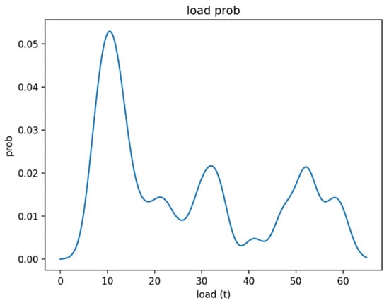
Figure 7.
Crane lifting load density function.
The load can be divided into three levels of light, medium and heavy, and the interval is [0, 15], [15, 40] and [40, 65]. With the obtained density function, we can calculate the probability of the crane lifting load in the range of 0 to 15 t as 66.10%; 15 to 40 t as 19.22%; 40 to 65 t as 14.45%; and the value of the 90% quantile as 50.2 t.
With this load classification, the energy consumption under different loads can be calculated separately. The main work of the crane is the lifting of the goods, that is, the up and down movement of the spreader. Through the derivation of the position value of the spreader, the speed of the spreader moving up and down can be obtained, and then multiplied by the load, the main energy consumption of the crane can be obtained.
Figure 8 shows the energy consumption for three load cases and the selected data are typical data obtained from subsequent experiments.
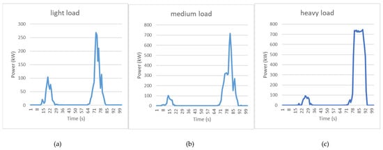
Figure 8.
Energy consumption under different loads: (a) light load, (b) medium load and (c) heavy load.
4.3. Typical Working Cycle of Trolley Speed
Due to the inevitable data drift and other phenomena in actual data, the speed data of the trolley needs to be preprocessed to correct for exception values and smooth the noise. Then, the feature value of the speed is calculated and standardized. Finally, the k-means algorithm is used with the number of clusters being set to one. The sample with the closest distance to the final cluster center is taken as the typical working cycle, shown in Figure 9, and the comparison between the typical working cycle eigenvalue and the average eigenvalue of all collected data is shown in Table 5.
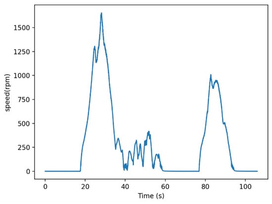
Figure 9.
Speed sequence diagram of typical working cycle.
Table 5.
Eigenvalue comparison of typical working cycle and the average values.
4.4. Clustering Analysis of Vibration Signals
First, in order to verify the effect of the unsupervised machine learning method proposed in this article in fault diagnosis, experiments are conducted with the publicly available data set from Case Western Reserve University.
This experiment selects the drive end data of a 14-inch bearing installed at a sampling frequency of 12 kHz. The bearing had an inner ring failure, a rolling element failure and a 6 o’clock outer ring failure at 1797 rpm.
Ten faulty samples were selected from each of the three groups of faulty data, in addition to 30 samples from each of the three corresponding groups of normal data to form a total data set of 90. When the final number of clusters is set to 4, the number of samples in each category is 60, 17, 12 and 1, as shown in Figure 10. Among them, 60 normal data are identified as one cluster, and the other clusters are faulty data, indicating that the method can achieve the separation of faulty data from normal data.
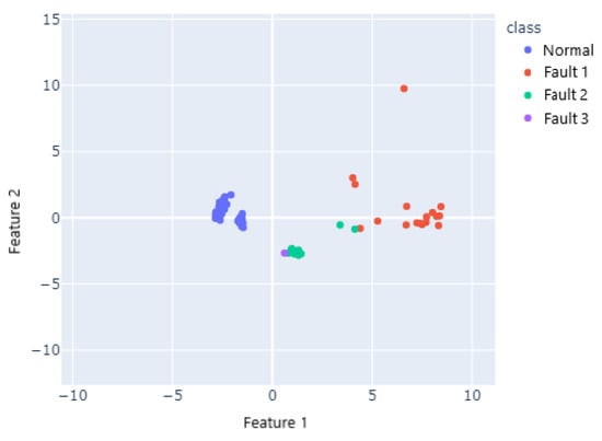
Figure 10.
Distribution of samples by cluster.
SSE (Sum of Squared errors) measures the similarity within each cluster and is often used as a quantitative evaluation of clustering algorithms. Because the k-means algorithm iterates quickly, and the results are greatly affected by the selection of the initial point, the k-means algorithm is generally executed multiple times to select the optimal result. Table 6 shows the variation of SSE in executing the k-means algorithm four times.
Table 6.
The variation of SSE.
Secondly, the data collected from the actual port machine will then be the object of the next experiment.
The data set contains a total of 16 vibration data points from sensors located in the gearbox, and this article uses the signals collected by the sensors on the output shaft of the crane hoist mechanism. Firstly, the time domain and frequency domain eigenvalues of the vibration signals were calculated; then, normalized and k-means clustering was performed. By setting different numbers of clusters and analyzing the clustering results, it was found that even when the number of clusters was greater than 1, the number of sample points in each category is still evenly distributed, which proved that the data set did not contain fault data. This conclusion is also consistent with the composition of the data set.
By setting different numbers of clusters, as shown in Figure 11, we can obtain multiple sets of data. The sample closest to the center can be treated as the typical vibration data that can represent this data set. Therefore, the typical data under different loads can be obtained by first grouping the data according to three load levels and then clustering them separately.
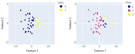
Figure 11.
The cluster result when the number of clusters is 2 and 3, respectively.
5. Discussion of the Results
The main purpose of this article is to address the difficulty in obtaining valuable information from the vast amount of information and excessive data storage pressure as ports become intelligent.
First, the load spectrum was obtained from the raw data by kernel density estimation. The load spectrum can be used as the basic condition for calculating the structural life. It can also intuitively show the cargo transportation situation for a period of time to the port operator, understand the proportion of different weights of cargo and provide a factual basis for formulating the follow-up development direction. In addition, the energy consumption under different loads is calculated. Based on the energy consumption curve, the smart port can dynamically adjust the working status of each crane to avoid the superposition of energy consumption peaks, thereby reducing energy bills and green gas emissions.
Secondly, the typical working cycle of the trolley is obtained from the massive data. As important as the problem of typical working cycle in the automotive field is, the acquisition of the working cycle of the trolley can guide the next development and selection. In addition, the working cycle of the trolley directly reflects the working efficiency of each crane. Comparing the typical working cycle of different cranes can help the port to further optimize the efficiency and provide a basis for berth allocation and crane operation optimization.
Finally, experiments with cluster analysis of gearbox vibration signals on a public data set have verified its validity, and the analysis results on real data are identical to the actual situation. As an effective anomaly detection method, cluster analysis of gearboxes can greatly reduce the frequency of manual inspections and further accelerate the intelligence of the port. In addition, by setting different filtering conditions and different number of clusters, multiple clustering results can be obtained, and then the centers of the different clusters can be stored separately as typical data. The rest of the data can be deleted, which not only completes the process of data analysis and extraction and ensures the integrity of typical historical data but also effectively reduces the pressure on the port to store several gigabytes of data per day.
6. Conclusions
This article proposes a framework and method for data mining using different sensor signals in smart harbors, which solves the problem of using, retaining and deleting massive amounts of data in smart ports. The load spectrum, energy consumption curve and typical working cycle of the trolley obtained in this article can help the port in its decision making and optimization from different aspects. The cluster analysis of gearbox vibration signals in this article can become a common method for port anomaly detection, and it can also filter out typical data to delete the remaining redundant data and reduce the pressure of data storage.
This article does not go into more depth in the area of scheduling and planning management in ports but mainly provides the basis for the next step of research. Future research can be done in areas such as berth allocation and crane operation optimization. In terms of health status detection, the main need of the port lies in abnormality detection, and further research can focus on fault diagnosis to achieve the discovery of abnormalities while locating faults.
Author Contributions
Conceptualization, Y.L., S.L. and Q.Z.; methodology, S.L.; software, S.L.; validation, Y.L., S.L. and Q.Z.; formal analysis, S.L.; investigation, Y.S.; resources, Y.L. and B.X.; data curation, S.L.; writing—original draft preparation, S.L.; writing—review and editing, Q.Z.; visualization, S.L.; supervision, Q.Z.; project administration, Y.L. and B.X.; funding acquisition, Y.L. and B.X. All authors have read and agreed to the published version of the manuscript.
Funding
The APC was funded by Guangzhou Port Group Co., Ltd.
Data Availability Statement
The data presented in this study are available on request from the corresponding author. The data are not publicly available due to commercial privacy issues.
Conflicts of Interest
The authors declare no conflict of interest.
References
- Muñuzuri, J.; Onieva, L.; Cortés, P.; Gaudix, J. Using IoT data and applications to improve port-based intermodal supply chains. Comput. Ind. Eng. 2020, 139, 105668. [Google Scholar] [CrossRef]
- Fruth, M.; Teuteberg, F.; Liu, S. Digitization in maritime logistics-What is there and what is missing? Cogent Bus. Manag. 2017, 4, 1411066. [Google Scholar] [CrossRef]
- Hu, S.; Fang, Y.; Bai, Y. Automation and optimization in crane lift planning: A critical review. Adv. Eng. Inform. 2021, 49, 101346. [Google Scholar] [CrossRef]
- Rodrigues, F.; Agra, A. Berth allocation and quay crane assignment/scheduling problem under uncertainty: A survey. Eur. J. Oper. Res. 2022, 202, 615–627. [Google Scholar] [CrossRef]
- Geng, S.; Liu, X.; Yang, X.; Meng, Z.; Wang, X.; Wang, Y. Load spectrum for automotive wheels hub based on mixed probability distribution model. Proc. Inst. Mech. Eng. Part D J. Automob. Eng. 2019, 233, 3707–3720. [Google Scholar] [CrossRef]
- Luo, J.; Wang, S.; Liu, X.; Geng, S. Fatigue life prediction of train wheel shaft based on load spectrum characteristics. Adv. Mech. Eng. 2021, 13, 2072368303. [Google Scholar] [CrossRef]
- Zhang, Y.; Kim, C.W.; Tee, K.F.; Lam, J.S.L. Optimal sustainable life cycle maintenance strategies for port infrastructures. J. Clean. Prod. 2017, 142, 1693–1709. [Google Scholar] [CrossRef]
- He, J.; Wang, Y.; Tan, C.; Yu, H. Modeling berth allocation and quay crane assignment considering QC driver cost and operating efficiency. Adv. Eng. Inform. 2021, 47, 101252. [Google Scholar] [CrossRef]
- Anida, I.N.; Salisa, A.R. Driving cycle development for Kuala Terengganu city using k-means method. Int. J. Electr. Comput. Eng. 2019, 9, 1780–1787. [Google Scholar] [CrossRef]
- Desineedi, R.M.; Mahesh, S.; Ramadurai, G. Developing driving cycles using k-means clustering and determining their optimal duration. Transp. Res. Procedia 2020, 48, 2083–2095. [Google Scholar] [CrossRef]
- Bishop, J.D.K.; Axon, C.J.; Mcculloch, M.D. A robust, data-driven methodology for real-world driving cycle development. Transp. Res. Part D Transp. Environ. 2012, 17, 389–397. [Google Scholar] [CrossRef]
- Brady, J.; O’Mahony, M. Development of a driving cycle to evaluate the energy economy of electric vehicles in urban areas. Appl. Energy 2016, 177, 165–178. [Google Scholar] [CrossRef]
- Wang, L.; Shao, Y. Crack Fault Classification for Planetary Gearbox Based on Feature Selection Technique and K-means Clustering Method. Chin. J. Mech. Eng. 2018, 31, 4. [Google Scholar] [CrossRef] [Green Version]
- Zhang, X.; Zhao, J.; Li, H.; Ni, X.; Sun, F. Gearbox Fault Diagnosis Based on Multifractal Detrended Fluctuation Analysis and Improved K Means Clustering. In Proceedings of the 2018 Prognostics and System Health Management Conference (PHM-Chongqing), Chongqing, China, 26–28 October 2018; pp. 527–531. [Google Scholar]
- Iris, Ç.; Lam, J.S.L. A review of energy efficiency in ports: Operational strategies, technologies and energy management systems. Renew. Sustain. Energy Rev. 2019, 112, 170–182. [Google Scholar] [CrossRef]
- He, J. Berth allocation and quay crane assignment in a container terminal for the trade-off between time-saving and energy-saving. Adv. Eng. Inform. 2016, 30, 390–405. [Google Scholar] [CrossRef]
- Geerlings, H.; Heij, R.; van Duin, R. Opportunities for peak shaving the energy demand of ship-to-shore quay cranes at container terminals. J. Shipp. Trade 2018, 3, 1–20. [Google Scholar] [CrossRef]
- Iris, Ç.; Lam, J.S.L. Optimal energy management and operations planning in seaports with smart grid while harnessing renewable energy under uncertainty. Omega 2021, 103, 102445. [Google Scholar] [CrossRef]
- Finite Mixture Models. Encyclopedia of Autism Spectrum Disorders; Volkmar, F.R., Ed.; Springer: New York, NY, USA, 2013; p. 1296. [Google Scholar]
- Chen, D.Y.; Sun, S.G.; Li, Q. A New Dynamic Stress Spectrum Distribution Estimation Method of High-speed Train. J. Mech. Eng. 2017, 53, 109–114. [Google Scholar] [CrossRef]
- Quan, Q.; Cai, K. Time-domain analysis of the Savitzky–Golay filters. Digit. Signal Process. 2012, 22, 238–245. [Google Scholar] [CrossRef]
- Shahidinejad, S.; Bibeau, E.; Filizadeh, S. Statistical Development of a Duty Cycle for Plug-in Vehicles in a North American Urban Setting Using Fleet In-formation. IEEE Trans. Veh. Technol. 2010, 59, 3710–3719. [Google Scholar] [CrossRef] [Green Version]
- Chang, J.; Li, T.; Li, P. The selection of time domain characteristic parameters of rotating machinery fault diagnosis. In Proceedings of the 2010 International Conference on Logistics Systems and Intelligent Management (ICLSIM), Harbin, China, 9–10 January 2010; pp. 619–623. [Google Scholar]
- Xue, X.; Zhou, J. A hybrid fault diagnosis approach based on mixed-domain state features for rotating machinery. ISA Trans. 2017, 66, 284–295. [Google Scholar] [CrossRef] [PubMed]
- Guo, W.; Zhao, H.; Gao, X.; Kong, L.; Li, Y. An efficient representative for object recognition in structural health monitoring. Int. J. Adv. Manuf. Technol. 2018, 94, 3239–3250. [Google Scholar] [CrossRef]
- Astakhova, N.N.; Demidova, L.A.; Nikulchev, E.V. Forecasting method for grouped time series with the use of k-means algorithm. Appl. Math. Sci. 2015, 9, 4813–4830. [Google Scholar] [CrossRef] [Green Version]
- Yiakopoulos, C.T.; Gryllias, K.C.; Antoniadis, I.A. Rolling element bearing fault detection in industrial environments based on a K-means clustering ap-proach. Expert Syst. Appl. 2011, 38, 2888–2911. [Google Scholar] [CrossRef]
Publisher’s Note: MDPI stays neutral with regard to jurisdictional claims in published maps and institutional affiliations. |
© 2022 by the authors. Licensee MDPI, Basel, Switzerland. This article is an open access article distributed under the terms and conditions of the Creative Commons Attribution (CC BY) license (https://creativecommons.org/licenses/by/4.0/).