A Bayesian Pipe Failure Prediction for Optimizing Pipe Renewal Time in Water Distribution Networks

Abstract

The sustainable management of the water supply system requires methodologies to monitor, repair, or replace the aging infrastructure, but more importantly, it must be able to assess the condition of the networks and predict their behavior over time. Among other infrastructure systems, the water distribution network is one of the essential civil infrastructure systems; therefore, the effective maintenance and renewal of the infrastructure’s physical assets are essential. This article aims to determine pipe failure prediction to optimize pipe renewal time. This research methodology investigates the most appropriate parameters for predicting pipe failure in the optimization. In particular, the non-homogeneous Poisson process (NHPP) with the Markov chain Monte Carlo (MCMC) approach is presented for Bayesian inference, while maximum likelihood (ML) is applied for frequentist inference as a comparison method. It is concluded that the two estimations are relatively appropriate for predicting failures, but MCMC estimation is closer to the total observed data. Based on life-cycle cost (LCC) analysis, the MCMC estimation generates flatter LCC curves and lower LCC values than the ML estimation, which affects the decision making of optimum pipe renewal in water distribution networks.

1. Introduction

The water distribution network (WDN) is one of the essential public infrastructure systems. It requires frequent inspection, occasional maintenance, and swift repairs throughout its service life to maintain its performance levels [1]. Therefore, it is essential to maintain effective maintenance and repair plans and to refresh the system’s physical assets, particularly in regions where widespread failure is possible. A complicated WDN is susceptible to failure and may result in the collapse of the pipeline, the failure of neighboring utilities such as underground electrical lines, the disruption of traffic and local economic activity, and even fatalities. Environmental variables, the age of the assets, and component deterioration may cause system failures. These faults can occur at any time, anywhere, and have a variety of threatening consequences for other infrastructure systems, such as transportation networks and building foundations [2].

The sensitivity of WDNs to failure is the driving force behind the deployment of asset management, which aims to achieve an optimal price and service level for customers. The most expensive component of the WDN is the pipeline utility. Pipe failure is affected by the fundamental properties of the utility, such as pipe material, diameter, length, age, and previous failure history. Establishing a correlation between the failure rate and these variables is essential for assessing network status and preventing catastrophic failure. In the WDN, decision makers must implement infrastructure asset management to ensure that infrastructure performance achieves service level, risk management, and cost management in the context of the asset life-cycle at the most cost-effective level. If asset management is a crucial component of any pipeline utility, then accurate information on the service life of the pipes is a crucial aspect of asset management. Understanding the current condition and remaining lifetime of a network gives numerous benefits, including optimizing hydraulic operation and maintenance techniques, reducing network expenses and costs, and identifying the optimal level of service [3].

Throughout its lifetime, the WDN may be subjected to unanticipated loading or lining conditions, which might cause pipe damage. The expected incidence of pipe failure for older water systems employing pipe materials such as asbestos–cement, cast iron, and ductile iron can be approximated by analyzing the considerable data associated with long previous failure records. On the other hand, for relatively new pipe materials, such as polyvinyl chloride (PVC), it is hard to make accurate predictions based on limited historical data [4]. Failure frequency tends to be biased when parameter estimation is not carried out properly, leading to selection bias for pipe feasibility. As the sample size increases, the uncertainty becomes smaller, while the bias remains constant [5]. This highlights the significance of applying an appropriate method to estimate the parameter values when evaluating brief failure data series. This article aims to determine pipe failure prediction to optimize pipe renewal time in the WDN. This research methodology investigates the most appropriate parameters for predicting pipe failure for optimization. In particular, the non-homogeneous Poisson process (NHPP) with Bayesian inference is used to predict pipe failure rates. In the following explanation, Bayesian inference is compared with frequentist inference. The Markov chain Monte Carlo (MCMC) approach is presented for Bayesian inference, while maximum likelihood (ML) is used for frequentist inference. We investigate how failure prediction can provide a cost-effective pipe renewal strategy and determine the most economical renewal lifetime. The model calculates the most cost-effective life-cycle costs based on the present value of renewal costs, repair costs, and predicted failure.

2. Literature Review

Pipe failure prediction is required for the development of preventative techniques in infrastructure management. Shamir and Howard’s [6] article on establishing the optimal pipe renewal time is a crucial source for determining the appropriate renewal interval. It comprised a deterministic model for optimizing the economic effectiveness of repair versus renovation times. Since then, deterministic, statistical, and machine learning methods have been applied in the research of pipe performance and resulting lifetime. Lauer [7] presented an excellent general strategy for network maintenance with insight into failure prediction. Rostum [8] offered a thorough statistical study of the pipe failure process based on the NHPP model. Kleiner et al. [9] proposed economies of scale into a model of pipe renewal, while Fuchs-Hanusch et al. [10] modified the pipe life-cycle equation by integrating leak detection costs that increase with pipe age. Scholten et al. [11] developed a failure model using the exponential–Weibull distribution. It was also used in multi-criteria decision analysis to rank various long-term rehabilitation alternatives. Amaitik et al. [12] supported using neural networks for failure prediction and pipe renovation, whereas Kabir [13] utilized a Bayesian framework to accomplish the same goal. Motiee et al. [14] examined four alternative regression models, Di Nardo et al. [15] applied fractal theory to evaluate the robustness of pipe failures, and Kutylowska [16] predicted pipe failure rates with support vector machines. Specifically, research on the Weibull proportional hazard model (WPHM) can be found in the works of Le Gat and Eisenbeis [17].

Giraldo-Gonzales and Martinez [6] exposed several statistical models, such as Poisson regression, linear regression, and EPR, to predict the number of pipe group failures. Due to their explicit polynomial expressions, which offer a decent correlation between covariates and dependent variables, these models are recommended. Linear regression is an extension of regression analysis that includes covariates as explanatory variables in the prediction equation. In the linear regression model, whether the value of the covariate increases or decreases, the value of the dependent variable changes at a constant rate. Consequently, the fundamental disadvantage of statistical models is their dependence on the availability of comprehensive data. Probabilistic statistical models need the development of a time-dependent failure rate function, in which the time until the next failure varies based on the conditions of the previous failure. Based on previous research, this can be achieved by performing the time-dependent Poisson model and the Markov process in conjunction with the Bayesian principle. Atique and Attoh-Okine [18] constructed a pipe failure model using Bayesian inference and the Copula parameter to describe bivariate distribution by sampling the distribution, including the dependent variable. Lin and Yuan [19] created an NHPP model and presented a two-scale process with two-time variables applying Markov chain Monte Carlo (MCMC).

The importance of asset management in urban water utilities continues due to their technological, economic, and environmental ramifications being substantial and numerous. Specifically, providing accurate estimates for the service life of pipes is a crucial component of the asset management problem. In Mailhot et al.’s [20] model, another optimization-based rehabilitation planning technique with a cost-conscious focus is considered as an indicator of the pipe’s structural integrity to calculate the best renewal criterion. Hong et al. [21] proposed an analytical approach for the optimal pipe renewal based on the annual cost as a proportion of the overall cost by lowering the total expected cost over a set service life. A mathematical model developed by Luong and Nagarur [22] can assist in determining whether to repair or replace the pipe and how to deploy maintenance expenditures most effectively. The optimization formulation’s objective function is the total system availability over the long term. Grigg [23] offered a risk-based approach to pipe renewal to avoid utilizing a suboptimal budget. Lansey et al. [24], Kim and Mays [25], and Shin et al. [8] established more cost-minimization-focused models. Other optimization models integrate system cost and reliability as competing objectives. Dandy and Engelhardt [26] developed a trade-off curve for reliability and cost for the effective pipe renewal option.

Notably, several researchers have implemented life-cycle cost (LCC) analysis in WDN. This powerful notion highlights the analytical tools that assist decision makers in making the most cost-effective choices among the options provided to them at various life-cycle stages and, therefore, with varying costs. Shamir and Howard [27] constructed an exponential relationship between a pipe failure rate and its age to calculate the pipe renewal interval that minimizes total repair and renewal costs. Lee et al. [28] classified every network object to give an inventory-based technique for the LCC analysis of a WDN. This methodology was created to assist decision makers in determining when and which WDN components require repair.

Marzouk and Osama [29] developed a method to assist decision makers in WDN management with their short-term and long-term plans. Four objective functions were considered: the risk index, the infrastructure condition, the level of asset service, and the LCC. The failure probability was simulated using a fuzzy Monte Carlo simulation. The research discovered that economic variables influenced asset failure results significantly, whereas pipe size influenced the overall failure consequence index. Jayaram and Srinivasan [28] suggested an innovative multi-objective approach for lowering LCC and improving network performance. Roshani and Filion [30] created the OptiNET model to reduce renewal time and pipe diameter while reducing LCC. Capital and operating expenses were evaluated as the goal function for determining the optimal renewal age. According to Frangopol and Soliman [31], LCC analysis could significantly reduce long-term expenditures while improving the resilience and sustainability of the infrastructure. Based on the LCC assessment, Ghobadi et al. [32] present a new pipe renewal scheduling strategy to smooth the investment time series for a large-scale WDN.

3. Materials and Methods

3.1. Study Area and Data Sources

This article proposes the Malang City Water Network, East Java Province, Indonesia, as a case study. As the second biggest urban water supply in East Java Province, the network serves an area of 110 km². The coverage of the number of customers currently reaches 98% of the population of the city, approximately 680,000 citizens, and consists of 171,000 customer junctions. The quantity of the water supply is 1525 L per second. The various types of pipes in the study area consist of galvanized iron (GI), asbestos–cement (AC), polyvinyl chloride (PVC), and high-density polyethylene (HDPE), with the attributes listed in the

Table 1. Water distribution pipe material in the study area.

Pipe Material	Length (km)	Year of Installation
AC	25.42	1986
GI	5.04	1990
PVC	1241.87	2002
HDPE	1047.71	2012

.

The main distribution network consists of PVC pipes, while AC and GI pipes are gradually being replaced with HDPE. The pipe failure database was created in 2012 as a recommendation from the cooperation program between the Malang City Public Water Works Company and AusAID for urban water development. The Malang City Public Water Works Company conducts reliability evaluations every 20 years on each type of pipe material based on the availability of sufficient pipe failure data. At this point, decision makers need a reliability analysis for PVC pipe materials that have reached the age of 20 years, which have reached 30% of the planned age for network operations. In this regard, the article’s scope is limited to analyzing PVC distribution network pipes. Although the PVC pipes were installed in 2002, the data availability begins in 2012 and concludes in 2021.

Table 2. Annual pipe failures of PVC pipes.

Period	Number of Pipe Failures	Average Diameter (mm)
2012	567	82.30
2013	569	87.88
2014	372	92.96
2015	459	82.04
2016	680	93.47
2017	380	107.70
2018	471	96.77
2019	595	105.92
2020	621	102.62
2021	688	92.71

shows annual pipe failures of PVC pipes in the study area.

3.2. Counting Process

The counting process can be used to determine the sequence of events or an uncertain process of events. A random variable, N(t), is the number of failure occurrences in the time interval (0, t). The process {N(t), t ≥ 0} is a stochastic process or is specifically referred to as a counting process, if [33]:

• N(t) ≥ 0.
• N(t) is an integer value.
• If s < t, then N(s) ≤ N(t).
• For s < t, [N(t)−N(s)] is the number of previous events in the interval (s, t).

Based on the characteristics, a system can be divided into a repairable and a non-repairable system. In the repairable system, the failed component can be repaired with several repair processes and it is unnecessary to replace the entire system. In the non-repairable system, the failed component must be replaced with a new component because the failed component cannot be repaired. In the WDN, pipe networks can be described as repairable components. In a repairable system, after the minimal repair is conducted, the failed system will function in the same condition as it was at the time of the last failure. The minimal repair assumes that the repair time is very short; only a small proportion of the system elements will be replaced in the repair process [34].

3.3. Poisson Process

When analyzing a repairable system, it is important to focus on the characteristics of the system’s pattern of successive failures. If the system demonstrates a trend (i.e., a tendency for failures to occur more frequently or less frequently), it is evident that non-stationary approaches must be employed. The non-homogeneous Poisson process (NHPP) is the most frequently used model to describe a trend in repairable systems [34].

If a component fails with an intensity function (λ), N is the number of events that arise from a failure in a time interval (0, t), and the number of failures that follow a Poisson distribution can be written as [35]:

$$\mathrm{p}\left(\mathrm{x}\right)=\mathrm{P}\left(\mathrm{N}=\mathrm{n}\right)=\frac{{\mathrm{e}}^{-\mathsf{\lambda }}{\mathsf{\lambda }}^{\mathrm{n}}}{\mathrm{n}!};\mathrm{n}=0,1,2,\dots$$

(1)

NHPP is a Poisson process with various intensity functions. In the WDN, NHPP is a simple model that can be applied to systems with decreasing or increasing failure rates. The failure events depend on a specific time interval, where the observation results in discrete data and between events are mutually independent. The intensity function of the Poisson regression is as follows [6]:

$$\mathsf{\lambda }=\exp ({\mathsf{\beta }}_0+{\mathsf{\beta }}_1{\mathrm{x}}_1+\cdots +{\mathsf{\beta }}_{\mathrm{i}}{\mathrm{x}}_{\mathrm{i}})$$

(2)

where β_i denotes the pipe failure parameter to be estimated and x_i represents the pipe failure variable.

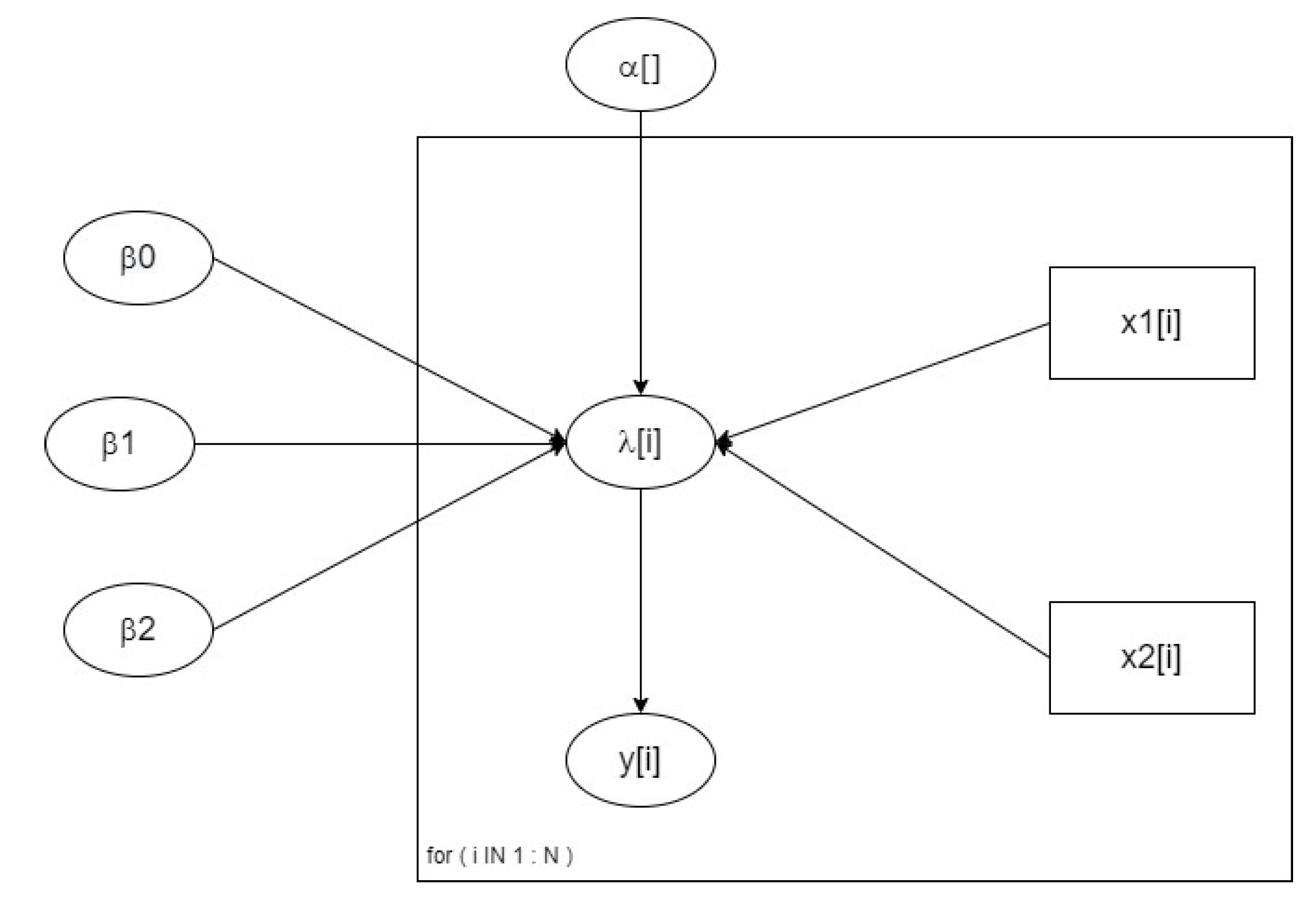
3.4. Bayesian Inference

Conceptually, the Bayesian method is based on the Bayes theorem, where the posterior distribution that is used to construct the likelihood function is a combination of prior distribution and observation data. The posterior distribution of $p\left(\lambda |x\right)$ can be determined using Bayes’ theorem to become [36]:

$$\mathrm{p}\left(\mathsf{\lambda }|\mathrm{x}\right)=\frac{\mathrm{p}\left(\mathrm{x}|\mathsf{\lambda }\right)\mathrm{p}\left(\mathsf{\lambda }\right)}{\mathrm{p}\left(\mathrm{x}\right)}$$

(3)

where $p\left(x|\lambda \right)$ is the likelihood function of the data containing the sample data information and can be written. Meanwhile,$p\left(\lambda \right)$ is the prior distribution function of the parameters and $p\left(x\right)$ is a constant density function.

The likelihood function is a representation of the data condition, while the determination of the prior distribution is more to the researcher’s subjectivity based on specific considerations. The specification of the prior distribution in Bayesian inference is also important, because the prior distribution will affect the inference of the posterior distribution. Determining the prior distribution is the key to inference analysis with Bayes and is the most important step in describing inference [36]. After the prior distribution is specified, the process to obtain the posterior distribution of the likelihood function and the prior distribution uses an analytical process or numerical integral, which is complicated to solve. In the Bayesian method, it can be solved using Markov chain Monte Carlo (MCMC). Through the MCMC method, it is possible to generate a sample from any posterior density function $p\left(\lambda |x\right)$ and then use the sample to calculate the expected value of the posterior [37].

The important thing in using MCMC is that if the simulation algorithm is implemented correctly, the Markov chain will converge to the particular distribution. The implementation of the MCMC method for Bayesian inference requires an appropriate sampling algorithm to obtain a sample from a distribution. Some of the algorithms developed for numerical processing in this MCMC method include the Gibbs sampling algorithm [37].

3.5. Maximum Likelihood Estimation

This article compares the Bayesian methodology with the frequentist inference, maximum likelihood (ML). L(θ;t) denotes the likelihood function when covariates are present. Consider the probability function to measure the likelihood that produced the observed T values. There is information provided for m independent observations with equal intensity function λ(t). Individual data i is monitored across the interval (ai, bi), and ni events are recorded at the intervals t_ij, where j = 1, 2, …, n_i and i = 1, 2, …, m. The likelihood function for all m processes is given by [38]:

$$\mathrm{L}\left(\mathsf{\theta };\mathrm{t}\right)=\prod _{\mathrm{i}=1}^{\mathrm{m}}[\prod _{\mathrm{j}=1}^{{\mathrm{n}}_{\mathrm{i}}}[\mathsf{\lambda }\left({\mathrm{t}}_{\mathrm{ij}}\right)]{\mathrm{e}}^{-{\int }_{{\mathrm{a}}_{\mathrm{i}}}^{{\mathrm{b}}_{\mathrm{i}}}\mathsf{\lambda }\left(\mathrm{u}\right)\mathrm{du}}]$$

(4)

The maximum likelihood estimation for pipe failures in the n events of failure, on the t time of failure, is expressed in the following equation [35]:

$$\mathsf{\lambda }=\frac{\mathrm{tn}}{{\mathrm{n}}^{-1/\mathsf{\beta }}}$$

(5)

which is:

$$\mathsf{\beta }=\frac{{\mathrm{n}}_1}{{\sum }_{\mathrm{i}=1}^{\mathrm{n}1}\ln \frac{\mathrm{tn}}{{\mathrm{y}}_{\mathrm{i},1}}}$$

(6)

The likelihood equations must be uniquely derived for a given distribution and estimation issue. Frequently, the mathematics is not simple, especially if confidence intervals for the parameters are required. Typically, the numerical estimation is not trivial. It is better to rely on high-quality statistical tools to produce maximum likelihood estimates, with a few exceptions where simple maximum likelihood formulas exist. Fortunately, the prevalence of high-quality maximum likelihood software is growing. For small samples, maximum likelihood estimates might be significantly biased, and it is possible that the optimality properties might not apply to small samples [39].

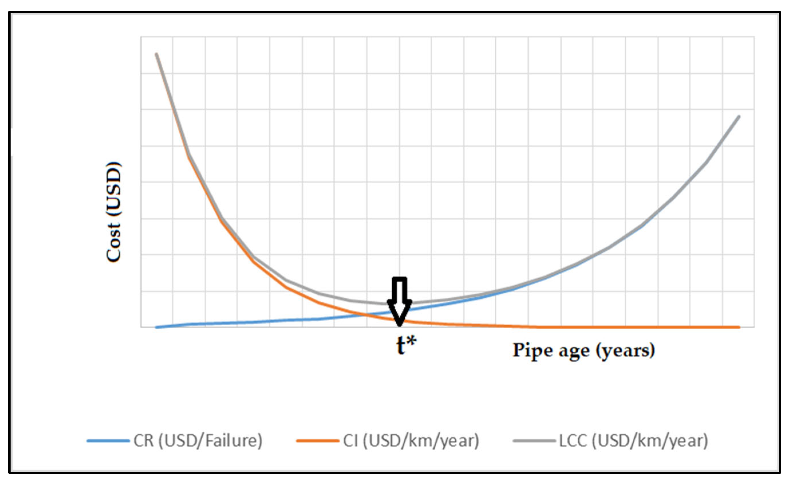
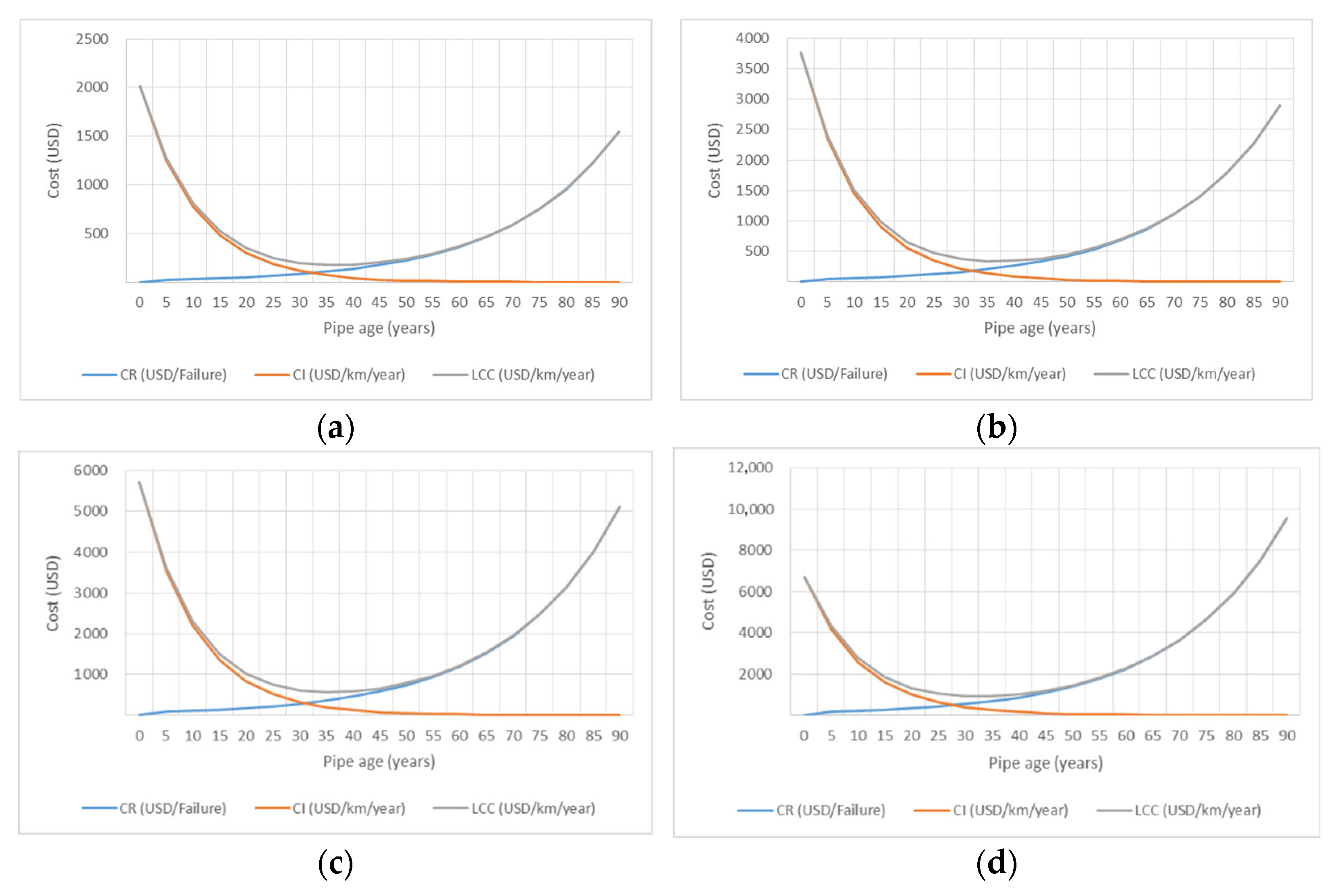
3.6. Life-Cycle Cost (LCC)

Life-cycle cost (LCC) is one of the most important factors to consider when determining the most cost-effective system solution. This article applies LCC evaluation to find the optimum time to replace the pipe. The LCC of a pipe network is the total of all costs incurred throughout its lifetime. Calculating the costs of procurement, operation, replacement, and disposal determines the LCC for each pipe attribute. This article uses the formula to calculate the LCC [32]:

$$\mathrm{LCC}=\mathrm{CI}+\mathrm{CR}$$

(7)

where D represents the pipe diameter (mm), CI represents the initial cost (USD/km/year), CR represents the running cost (USD/failure), and t is the pipe renewal interval (year). In this article, the CI only includes the procurement cost and the CR only includes the repair cost. The CI is expressed as follows [32]:

$$\mathrm{CI}=\frac{\mathrm{CP}}{\mathrm{t}}$$

(8)

where CP denotes the cost of pipe procurement (USD/km). Repair cost multiplied by the average failure rate throughout the renewal interval yields the CR and is expressed as follows [32]:

$$\mathrm{CR}=\frac{{\sum }_1^{\mathrm{t}}\mathrm{Fr}}{\mathrm{t}}\mathrm{Cr}$$

(9)

where Cr is the pipe repair cost (USD/failure) and Fr is pipe failure rate (failure/km/year), which is determined from the failure analysis.

Determining the LCC for each pipe feature enables the most cost-effective prediction of pipe age. Figure 1 shows an illustration of the LCC curve, presented with the pipe age, where operating costs increase while initial costs decrease. The lifetime with the lowest total cost is the most cost-effective. The lowest LCC for a particular pipe is referred to as the optimum LCC. The LCC curve provides the advantage of anticipating the ideal economic renewal time (t*) and displays the variation in total costs around this point. As shown in Figure 1, the renewal period should be adjusted within a time interval centered on the ideal point (t*) of the annual investment time series [32].

4. Results and Discussion

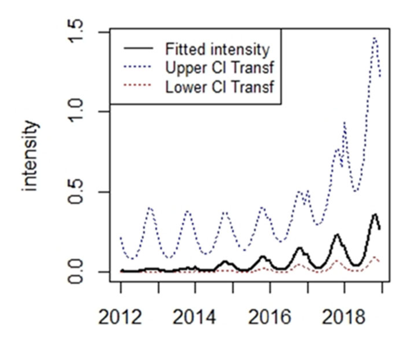
4.1. Pipe Failure Intensity

The analysis of pipe deterioration in the WDN, which is assumed to be a repairable system, focuses on observing the characteristics of failure patterns that occur successively. In this article, the modeling of pipe deterioration uses NHPP as a non-stationary approach. The counting process is applied to analyze the number of failures in an interval of failure time. Using an alpha level of 5%, the chi-squared test for homogeneity yields a chi-square value of 162.03 and a p-value of 2.2 × 10⁻¹⁶. Based on the examination results, it can be determined that the failure intensity is an inhomogeneous Poisson process with monthly failure intensity is shown in Figure 2.

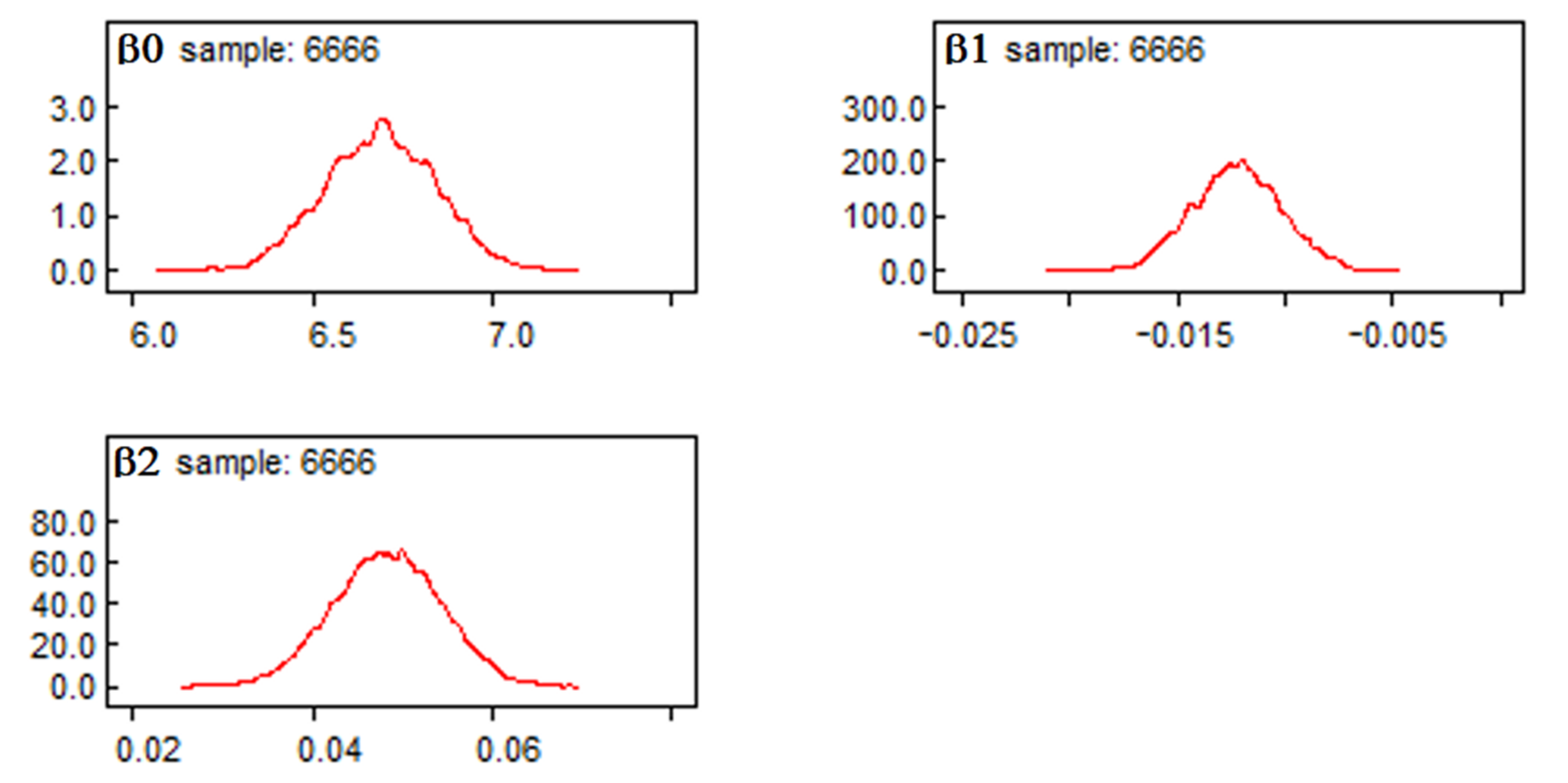
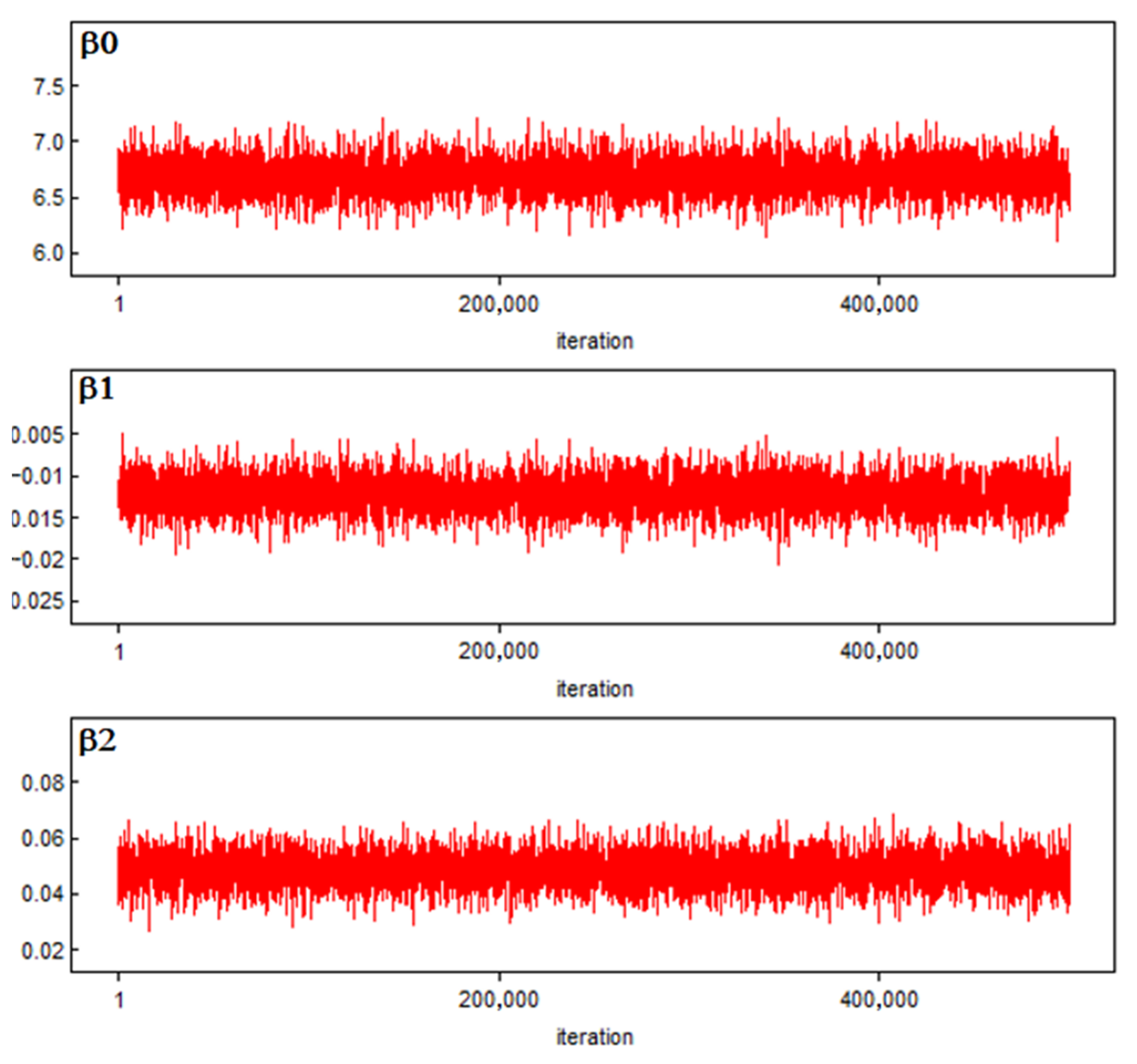
4.2. Parameter Estimation of Bayesian Inference

In Bayesian inference, a directed acyclic graph (DAG) can graphically represent the relationship between the data and the prior distribution of parameters. The DAG in Figure 3 depicts the relationship between the data, model parameters, and parameter values. In the graph, a single line represents a stochastic relationship. The box-shaped node represents constant parameters or data, whereas the elliptical node represents stochastically changing parameters or logical structural linkages. This article proposes pseudo prior in determining the prior distribution parameter to ensure that the parameter estimation process iterates rapidly and complies with the Markov chain. The posterior distribution determines model parameters using the MCMC method and Gibbs sampling algorithm. The results must be irreducible, aperiodic, and recurrent, as evidenced by the autocorrelation plot, the history plot, and the kernel density plot, respectively.

The model is examined by enumerating the significant contributions of each predictor variable according to whether the zero value falls within the credible interval of its posterior distribution. The form of the λ equation developed from Equation (2) with predictor variables is as follows:

$$\mathsf{\lambda }=\exp \left({\mathsf{\beta }}_0+{\mathsf{\beta }}_1\mathrm{D}+{\mathsf{\beta }}_2\mathrm{A}\right)$$

(10)

where D represents the variable of pipe diameter (in mm) and A represents the variable of pipe age (in years).

Table 3. MCMC parameter estimation result.

Parameter	Mean	Standard Deviation	2.5%	Median	97.5%
β0	6.69	0.1561	6.387	6.691	6.99
β1	−0.001222	0.002068	−0.01617	−0.01221	−0.008135
β2	0.04833	0.006018	0.03645	0.04839	0.05966

shows the MCMC estimation results for each parameter β0, β1, and β2.

All predictor variables are used simultaneously to model, resulting in the Bayesian model equation:

$$\lambda =exp\left(6.69-0.01222D+0.04833A\right)$$

(11)

The findings revealed a positive association between pipe failure rate and pipe age, as well as a negative relationship between pipe failure rate and pipe diameter.

In Figure 4, the autocorrelation plot shows that the correlation between the generated sample values is in the posterior distribution area.

Figure 5 depicts the estimated kernel density functions. The solid lines in the DAG depict these functions, respectively. Furthermore, the parameter estimate generated from this replication is calculated using the arithmetic mean in the density functions. The kernel density plot in Figure 5 shows that the posterior density for the model parameters gives a bell shape, following the distribution pattern of the model parameters. It is an indication that the Markov chain is convergent and consistent with the results of previous research [40].

Figure 6 depicts the results of the history plot on the MCMC simulation process. According to the figure, the history plot is stationary and random. It signifies that all of the generated samples fall within a specific domain interval. It is dense and contains all conceivable parameter values. The history plot is judged to be irreducible. This graphically depicts the chains’ rapid convergence and, as a result, verifies the MCMC technique’s usefulness. Iriawan and Yasmirullah [40] proposed that it is self-evident that using the MCMC approach will increase the parameter estimation accuracy and provide the empirical standard error that will be utilized to evaluate variability.

4.3. Parameter Estimation of Frequentist Inference

This article proposes the frequentist inference, maximum likelihood (ML), to be compared with MCMC.

Table 4. ML parameter estimation result.

Parameter	Estimate	Standard Error (SE)
β0	6.88818	0.1557
β1	−0.01489	0.0021
β2	0.051891	0.0059

shows the ML estimation results for each parameter β0, β1, and β2 with standard error (SE).

By substituting the estimated parameters into Equation (10), the intensity function of ML is as follows:

$$\mathsf{\lambda }=\exp \left(6.88818-0.01489\mathrm{D}+0.051891\mathrm{A}\right)$$

(12)

If we compare the two equations generated from MCMC and ML, it can be seen that although the parameters have different values, they tend to have the same relationship with the pipe failures. The relationship between pipe diameter and pipe failure is negative, while the age of the pipe has a positive relationship. This result is consistent with previous pipe failure analysis findings by several researchers [41,42].

According to the two equations generated by MCMC and ML, the diameter of the pipe correlates negatively with the number of failures, which is consistent with earlier studies [4,11,30]. The methods used by Giraldo-Gonzales et al. [8] revealed a negative association between diameter and rate of failure. The latter is because the deterioration process of pipes varies depending on the material. Construction methods, corrosion processes, and climatic variables can all have an impact on the link between pipe age, diameter, and failure rate. Many other elements, such as water pressure, rainfall near the pipe, and soil type, might influence the occurrence of pipe faults [3]. Pipes with a smaller diameter typically fail at a higher rate than bigger ones. The increased failure rate of small-diameter pipes is mostly due to the pipe’s reduced resistance to soil movement and corrosion as a result of reduced wall thickness.

Pipe deterioration due to age is a well-known phenomenon. Older pipelines fail at a higher rate. The failure rate is projected to rise in the months following installation, then fall for several years before rising with the pipe age [43]. Due to the production phase, on-site placement and operating practices, and external circumstances, the relationship between the age of a pipe and its failure rate is unknown. However, this could be explained by the fact that some pipes are older than when the first pipe failures were recorded [44]. Other authors have noted that the models only consider quantitative factors as the cause of this result. Changes in material quality and material strength may lead to age-dependent differences in pipe performance; however, these variables are not evaluated [6]. Other researchers [45,46,47] discovered variations in the fitted values of the variables between materials. The observed failure occurrences were influenced by the specified parameters and the age of the pipe. It is important to realize that as the pipeline ages, the failure rate will increase, and the model structure may need to be modified. It is relevant to Xu et al.’s [48] notation that no reliable model is applicable to every case.

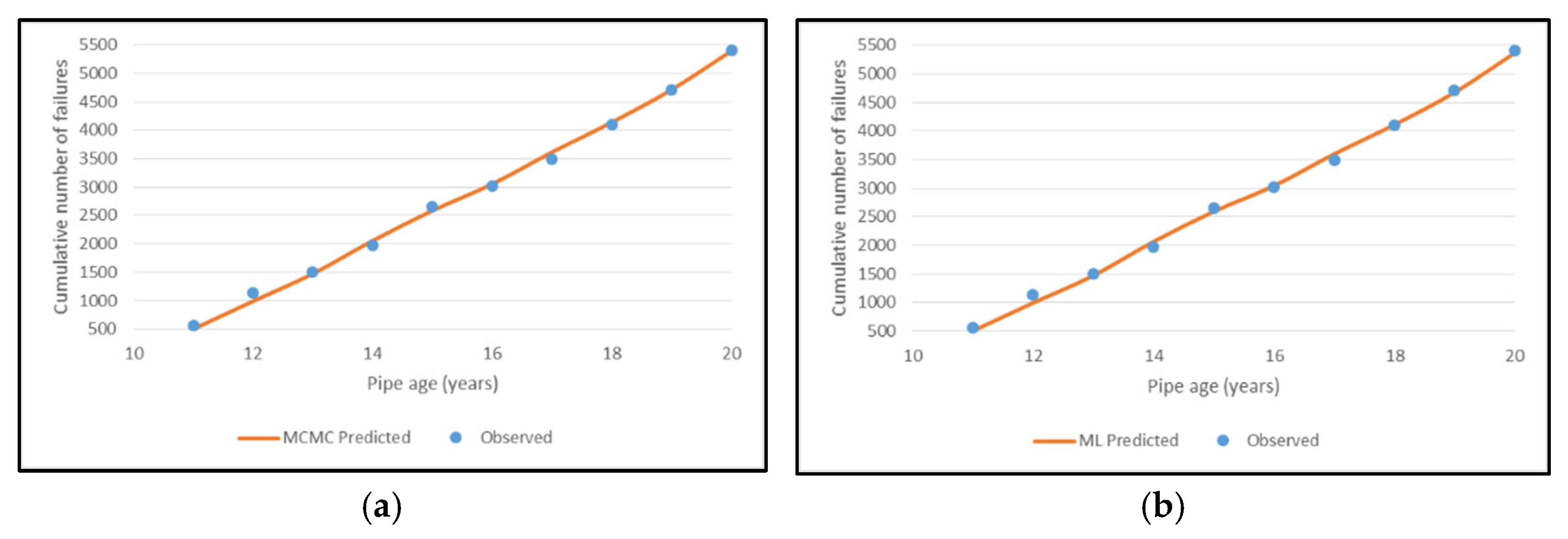
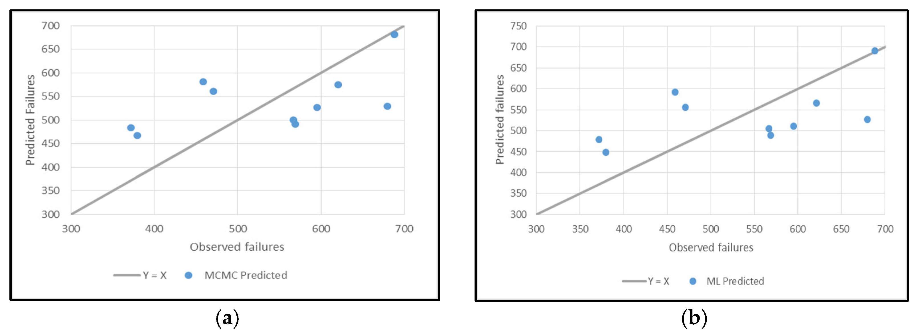
4.4. Pipe Failure Analysis

In the next step, we perform a pipeline failure analysis based on the pipe failure model.

Table 5. Annual number of pipe failures.

Period	Observed	MCMC Predicted	ML Predicted
2012	567	501	505
2013	569	491	490
2014	372	484	478
2015	459	581	593
2016	680	530	527
2017	380	467	449
2018	471	561	556
2019	595	526	511
2020	621	575	566
2021	688	681	690
Total	5402	5396	5365

shows the predicted annual pipe failure values compared to the observed values. From the analysis results, the model shows a lower number of failures in the early years, a larger number of failures in the middle years, and a lower number of failures in the later years. The model tends to have a middle rating of the peak number of failures indicated by the observation data. On the other hand, we discover that the number of failures between the MCMC and ML estimation is not significantly different, despite the fact that MCMC estimation is closer to the observed data.

We use a graph depicting the number of expected failures and observed failures for each year to evaluate the model’s accuracy. Figure 7 and Figure 8 illustrate the pipe failure plot over time. The total numbers of predicted and observed failures are comparable, and it is exciting to observe the model’s performance in the event of failure. In this evaluation, cumulative and annual charts are practical visual assessment techniques. Annual plots can be utilized to compare model outcomes to actual failures visually. This plot can also depict the inter-failure time trend of the networks [49].

The following step compares the observed and predicted failures by scattering the predicted failures to the failure pair plot. An appropriate model is one in which the Y=X line is shown around the scattered predicted failures. From Figure 9, it can be seen that both models produce predictive values that are not much different from the observed values, which can be seen from the distribution of the predicted values around the Y=X line.

Another method for validating pipe failure prediction is to run tests on each quartile of the pipe failures. The predictive data for a period are validated using observational data from the same quartile in this test. If a model is applied to a pipeline life phase, it should be able to identify the pipeline with the highest failure quartile. If the predicted pipe has the highest likelihood of failure and the observational data demonstrate the same thing, the model should be judged valid for the pipe’s service life [49]. The quartile results are displayed in the following table.

Table 6. Quartile of the pipe failures with MCMC estimation.

Failure Quartile	Observed	Predicted	Margin (%)
1st Quartile	1191	1441	−20.93
2nd Quartile	1059	1030	2.68
3rd Quartile	1799	1665	7.43
4th Quartile	1353	1260	6.87
Total	5402	5396	0.10

and 7 demonstrate that the both models are relatively appropriate at predicting failure in each quartile. There is a tendency for the predicted failures to be consistent with the observed failures. Table 6 and

Table 7. Quartile of the pipe failures with ML estimation.

Failure Quartile	Observed	Predicted	Margin (%)
1st Quartile	1191	1414	−18.71
2nd Quartile	1059	1027	2.97
3rd Quartile	1799	1648	8.40
4th Quartile	1353	1276	5.67
Total	5402	5365	0.68

show that most of the failures occurred in the first quartile, with fewest occurring in the second.

It is critical to highlight that the failure rate examines the group of pipes rather than the history of pipe failure for each pipe [6]. The group of pipes in the first quartile has the highest priority for renewal. From previous research, prediction models developed with unbalanced data sets will have a greater tendency to anticipate the number of errors, which can reduce the prediction accuracy. The solution to this problem is to extend the length of the data series by accumulating errors over a longer period of time [50]. The water utility manager must monitor and take appropriate precautions, for example, maintenance or renewal after inspection. When there is no information about variables other than pipe features, the described method for predicting pipe failure is reasonably applicable. Selecting the proper group size depending on the data attributes is recommended [51].

The prediction validation, according to Ramirez et al. [7], should be conducted by examining and projecting the previous data and then comparing the earlier years of the projection with the more recent failure data. Scheidegger et al. [52] showed that there is no preferred model structure. The following points should be considered when selecting the most appropriate failure model: the appropriate probability function should be selected based on the data properties, the model estimate must correlate with the original inquiry, and the failure model assumptions must be consistent with operator experience [53].

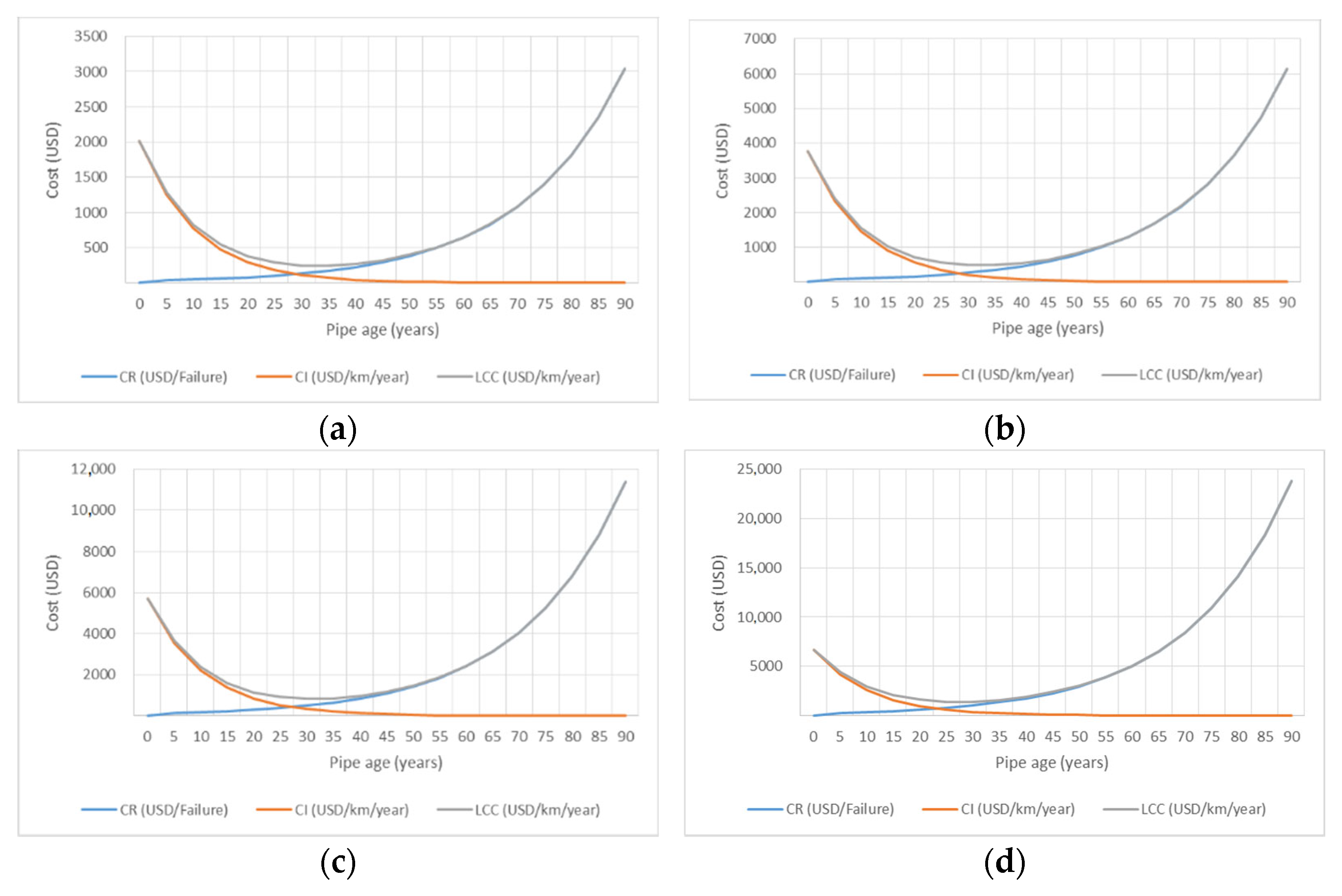
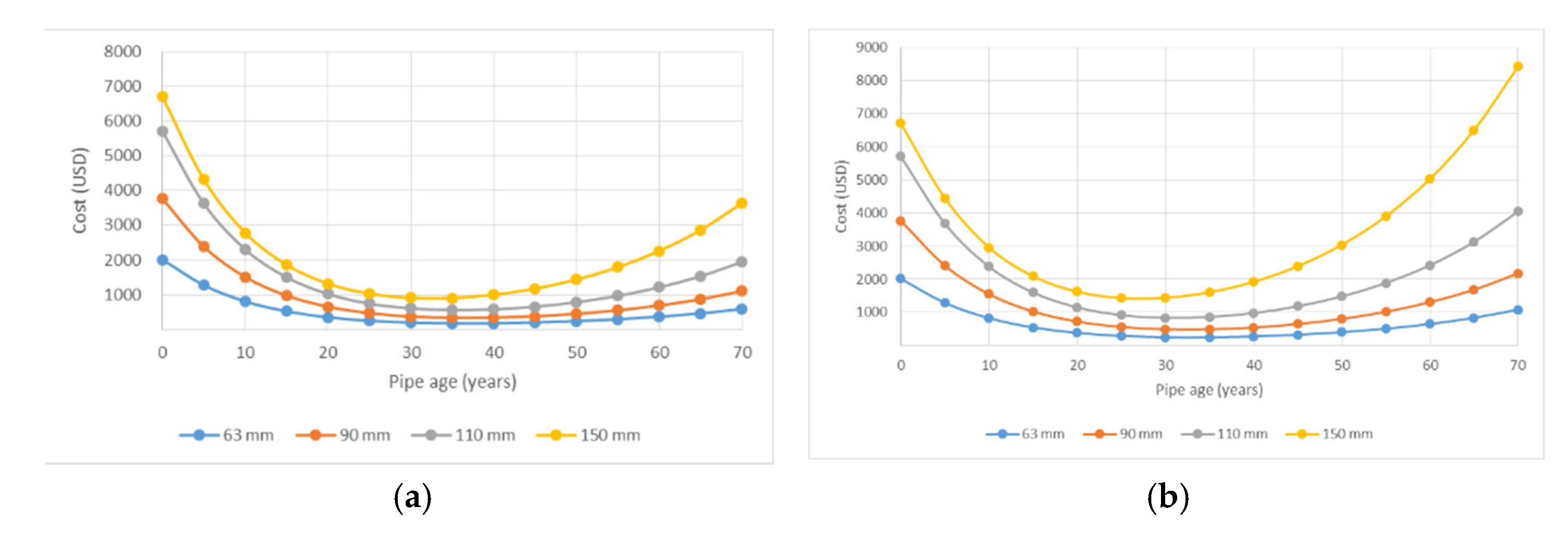
4.5. Life-Cycle Cost (LCC) Analysis

The LCC analysis can support the WDN authority to decide an efficient and cost-effective relocation strategy [25]. Figure 10 shows the LCC analysis from the MCMC estimation. Although the initial cost (CI) is different for each diameter, the trend decreases and flattens as the pipe age approaches 50 years. At the age of the pipe above 30 years, the running cost (CR) takes over the total cost, depending on the pipe failure rate from the pipe failure analysis results. The higher the pipe failure rate, the more the point of intersection of the CI and CR curves will shift to the left. This condition is similar to the optimal value of the LCC, where the higher the failure rate, the more the optimal point will shift to a shorter age. Based on the lowest LCC curve value for each diameter, the optimal pipe renewal time is obtained at the age of 35 years.

Figure 11 depicts the LCC analysis from the ML estimation and shows that the lowest LCC value is in the lifetime range of 25 to 35 years. At diameters of 63 mm and 90 mm, the lowest LCC is at the age of 35 years. When the pipe diameter is 110 mm, the lowest LCC is at the age of 30 years, and this increases for the pipe diameter of 150 mm, where the lowest LCC is in the age range of 25 years. As the diameter increases, the optimum lifetime decreases. The LCC analysis shows a different trend from the MCMC parameter estimation results. However, the ML estimation results for pipe diameters of 63 mm and 90 mm show the optimum pipe age values, which are relatively identical to the MCMC estimation results. If we look at the value of LCC in the same pipe age period, the ML estimation results show a higher value, and this difference becomes more significant as the time variable increases, even though the analysis in both models is conducted with the same value of cost components. The difference, in this case, is the pipe failure rate from the estimation results. Overall, the ML estimation produces higher LCC values and a shorter optimum pipe lifetime than the MCMC estimation.

If the total cost curve flattens around the optimal age, the decision makers do not need to schedule renewal exactly at that age (t*). If the LCC curve is uneven and fluctuating on both sides of the optimal age, repositioning should be conducted as near as possible to the optimal age. If the LCC curve is uneven and deviates significantly from the optimal point, renewal should be undertaken as near as is feasible to the optimal age. Modifying the renewal interval will affect the overall system life. Figure 12 depicts LCC curves, with each representing a different pipe diameter. With MCMC estimation, the smaller the pipe diameter, the flatter the LCC curve tends to be. Optimal pipe renewal decisions regarding pipes with a diameter of 63 mm, 90 mm, and 110 mm can be more relaxed compared to pipes with a diameter of 150 mm. Overall, the LCC curves of MCMC estimation is flatter than ML estimation at the same diameter. The ML estimation does not give the decision makers much choice in modifying the renewal interval. Figure 12 demonstrates that the LCC curves of ML estimation is more “pessimistic” than the MCMC estimation. This is represented by the uneven value of the costs around point t* on the LCC curves, as decision makers replace the pipe in a shorter time to prevent the possibility of more significant losses.

In the LCC analysis, there is a clear trade-off between two constraints: increasing the limitation on the renewal time may reduce the budget limit, and setting a time restriction for renewal impacts on the ability to adhere to budgetary constraints. It is important to determine how different budgets and time constraints will impact the target functions. The combination of the highest budget constraint and the lowest renewal limit leads to the lowest-cost scheduling plan with the lowest LCC [32].

Regarding diameter, Figure 12 shows that the pipe failure rate increases as the diameter of the pipe increases, although the diameter has a negative effect on the number of failures, referring to the model equations produced by the two estimation methods. However, Asnaashari et al. [54] and Harvey et al. [55] discovered that pipe diameter is less important than other factors, such as failure history and year of construction. In this case, the equations generated by both estimation methods are more positively affected by the age of the pipe. However, at the initial age of the pipe, the diameter still has a large influence, and then at a later age, the effect of diameter is less significant in terms of the number of failures. This affects the optimum pipe renewal time. In conditions where the diameter parameter has a more significant effect or is at least the same as the age parameter, it will give a longer renewal time for a larger diameter. In the LCC curves of the MCMC estimation, the tendency for longer renewal times for larger diameters is relatively invisible, and the renewal time is the same for all diameters. Different results are shown by the LCC curves of the ML estimation, where the LCC curves tend to be more uneven, and the renewal time for 110 mm and 150 mm is shorter than for 63 mm and 90 mm.

5. Conclusions

This article aims to determine pipe failure prediction to optimize WDN renewal. This research methodology investigates the most appropriate parameters for predicting pipe failure for optimization. The non-homogeneous Poisson process (NHPP) with Bayesian inference is used to predict pipe failure numbers. In the following explanation, Bayesian inference is compared with frequentist inference. The Markov chain Monte Carlo (MCMC) approach is presented for Bayesian inference, while maximum likelihood (ML) is used for frequentist inference. We investigate how failure prediction can provide a cost-effective pipe renewal strategy and determine the most economical renewal lifetime. The model calculates the most cost-effective life-cycle costs based on the NPV value of renewal costs, repair costs, and predicted failure.

The counting process is applied to analyze the number of failures in an interval of failure time. Based on the homogeneity examination, it can be determined that the failure intensity is inhomogeneous. From the two equations generated from the MCMC and ML estimation, it can be seen that although the parameters have different values, they tend to have the same relationship with the pipe failures. Pipe diameter and pipe failure have a negative relationship, whereas pipe age has a positive relationship. This result is consistent with earlier pipe failure analysis findings by several researchers. The failure prediction model tends to have a middle rating of the peak number of failures indicated by the observation data. On the other hand, we discover that the number of failures between the MCMC and ML estimation is not significantly different, despite the fact that MCMC has a higher total number of failures, which is closer to the observed data. The total number of predicted and observed failures are comparable, and it is exciting to observe the model’s performance in the event of failure. There are some apparent errors among the observed values and those predicted by MCMC and ML. Related to this, the MCMC predictions are better than the ML predictions because it MCMC has a lower mean squared error (MSE) value.

This article also proposes visual assessment techniques for evaluating the model concerning the resulting errors. In this evaluation, cumulative and annual charts are practical visual assessment techniques that can be used to compare model outcomes to actual failures visually. From pair plot validation, both models produce predictive values that are not much different from the observed values, which can be seen from the distribution of the predicted values around the Y=X line. The table demonstrates that the model is relatively appropriate at predicting failure in each quartile. There is a tendency for the predicted failures to be consistent with the observed failures. The pair plot shows that most of the failures occurred in the first quartile, and fewer occurred in the second. It is critical to highlight that the failure rate examines the group of pipes rather than the history of pipe failure for each pipe. The group of pipes in the first quartile has the highest priority for renewal. From the previous research, prediction models developed with unbalanced data sets will have a greater tendency to anticipate the number of errors, which can reduce the prediction accuracy. The solution to this problem is to extend the length of the data series by accumulating errors over a longer period of time. Based on the analysis, the recommended model is appropriate for predicting failure with serial data from ten years. Pipe failure predictions should be more accurate in situations with more than ten years of data.

The LCC analysis of the MCMC estimation has shown some points; although the initial cost (CI) is different for each diameter, the trend decreases and flattens as the pipe age approaches 50 years. At the age of the pipe above 30 years, the running cost (CR) takes over the total cost, depending on the pipe failure rate from the pipe failure analysis results. The higher the pipe failure rate, the more the point of intersection of the CI and CR curves will shift to the left. This condition is similar to the optimal value of LCC, where the higher the failure rate, the more the optimal point will shift to a shorter age. Based on the lowest LCC curve value for each diameter, the optimal pipe renewal time is obtained at the age of 35 years. The LCC analysis of the ML estimation shows that the lowest LCC value is in the pipe age range of 25 to 35 years. At diameters of 63 mm and 90 mm, the lowest LCC is at the age of 35 years. When the pipe diameter is 110 mm, the lowest LCC is at the age of 30 years, and it increases at the pipe diameter of 150 mm, where the lowest LCC is in the age range of 25 years. As the diameter increases, the age of the pipe decreases. The LCC analysis shows a different trend to the MCMC parameter estimation results. However, the ML estimation results for pipe diameters of 63 mm and 90 mm show the optimum pipe lifetime are relatively identical to the MCMC estimation results. If we look at the value of the LCC in the same pipe age period, the ML estimation results show a higher value, and this difference will be more significant as the time variable increases, even though the analysis in both models is conducted with the same value of cost components. The difference, in this case, is the pipe failure rate from the estimation results. The MCMC estimation results generally produce a lower LCC and a slightly longer optimum pipe life than the ML estimation. This will affect the decision making regarding pipe renewal in WDNs.

References

1. Mazumder, R.K.; Salman, A.M.; Li, Y.; Yu, X. Performance Evaluation of Water Distribution Systems and Asset Management. J. Infrastruct. Syst. 2018, 24, 03118001. [Google Scholar] [CrossRef]
2. Shuang, Q.; Liu, Y.; Liu, J.; Chen, Q. Serviceability Assessment for Cascading Failures in Water Distribution Network under Seismic Scenario. Math. Probl. Eng. 2016, 2016, 1431457. [Google Scholar] [CrossRef] [Green Version]
3. Pathirana, A.; den Heijer, F.; Sayers, P.B. Water Infrastructure Asset Management Is Evolving. Infrastructures 2021, 6, 90. [Google Scholar] [CrossRef]
4. Dawood, T.; Elwakil, E.; Mayol Novoa, H.; Fernando Gárate Delgado, J. Pressure data-driven model for failure prediction of PVC pipelines. Eng. Fail. Anal. 2020, 116, 104769. [Google Scholar] [CrossRef]
5. Barton, N.A.; Hallett, S.H.; Jude, S.R.; Tran, T.H. An evolution of statistical pipe failure models for drinking water networks: A targeted review. Water Supply 2022, 22, 3784–3813. [Google Scholar] [CrossRef]
6. Giraldo-González, M.M.; Rodríguez, J.P. Comparison of Statistical and Machine Learning Models for Pipe Failure Modeling in Water Distribution Networks. Water 2020, 12, 1153. [Google Scholar] [CrossRef] [Green Version]
7. Ramirez, R.; Torres, D.; López-Jimenez, P.A.; Cobacho, R. A Front-Line and Cost-Effective Model for the Assessment of Service Life of Network Pipes. Water 2020, 12, 667. [Google Scholar] [CrossRef] [Green Version]
8. Shin, H.; Kobayashi, K.; Koo, J.; Do, M. Estimating burst probability of water pipelines with competing hazard model. J. Hydroinform. 2016, 18, 126–135. [Google Scholar] [CrossRef] [Green Version]
9. Kleiner, Y.; Nafi, A.; Rajani, B. Planning renewal of water mains while considering deterioration, economies of scale and adjacent infrastructure. Water Supply 2010, 10, 897–906. [Google Scholar] [CrossRef]
10. Fuchs-Hanusch, D.; Kornberger, B.; Friedl, F.; Scheucher, R.; Kainz, H. Whole of life cost calculations for water supply pipes. Water Asset Manag. Int. 2012, 8, 19–24. [Google Scholar]
11. Scholten, L.; Scheidegger, A.; Reichert, P.; Mauer, M.; Lienert, J. Strategic rehabilitation planning of piped water networks using multi-criteria decision analysis. Water Res. 2014, 49, 124–143. [Google Scholar] [CrossRef]
12. Amaitik, N.M.; Amaitik, S.M. Prediction of pipe failures in water mains using artificial neural network models. In Proceedings of the 11th International Arab Conference of information Technology (ACIT’2010), University of Garyounis, Benghazi, Libya, 14–15 December 2010; pp. 1–8. [Google Scholar]
13. Kabir, G. Planning Repair and Replacement Program for Water Mains: A Bayesian Framework. Ph.D. Thesis, University of British Columbia, Vancouver, BC, Canada, 2016. [Google Scholar]
14. Motiee, H.; Ghasemnejad, S. Prediction of pipe failure rate in Tehran water distribution networks by applying regression models. Water Supply 2019, 19, 695–702. [Google Scholar] [CrossRef] [Green Version]
15. Di Nardo, A.; Di Natale, M.; Giudiciann, C.; Greco, R.; Santonastaso, G.F. Complex network and fractal theory for the assessment of water distribution network resilience to pipe failures. Water Supply 2018, 18, 767–777. [Google Scholar] [CrossRef]
16. Kutyłowska, M. Forecasting failure rate of water pipes. Water Supply 2019, 19, 264–273. [Google Scholar] [CrossRef] [Green Version]
17. Le Gat, Y. Extending the Yule process to model recurrent pipe failures in water supply networks. Urban Water J. 2014, 11, 617–630. [Google Scholar] [CrossRef]
18. Atique, F.; Attoh-Okine, N. Copula parameter estimation using Bayesian inference for pipe data analysis. Can. J. Civ. Eng. 2018, 45, 61–70. [Google Scholar] [CrossRef] [Green Version]
19. Lin, P.; Yuan, X.-X. A two-time-scale point process model of water main breaks for infrastructure asset management. Water Res. 2019, 150, 296–309. [Google Scholar] [CrossRef]
20. Mailhot, A.; Poulin, A.; Villeneuve, J.-P. Optimal replacement of water pipes. Water Resour. Res. 2003, 39, 1136. [Google Scholar] [CrossRef] [Green Version]
21. Hong, H.P.; Allouche, E.N.; Trivedi, M. Optimal Scheduling of Replacement and Rehabilitation of Water Distribution Systems. J. Infrastruct. Syst. 2006, 12, 184–191. [Google Scholar] [CrossRef]
22. Luong, H.T.; Nagarur, N.N. Optimal Maintenance Policy and Fund Allocation in Water Distribution Networks. J. Water Resour. Plan. Manag. 2005, 131, 299–306. [Google Scholar] [CrossRef]
23. Grigg, N.S. Water Main Breaks: Risk Assessment and Investment Strategies. J. Pipeline Syst. Eng. Pract. 2013, 4, 4013001. [Google Scholar] [CrossRef]
24. Lansey, K.E.; Basnet, C.; Mays, L.W.; Woodburn, J. Optimal Maintenance Scheduling for Water Distribution Systems. Civ. Eng. Syst. 1992, 9, 211–226. [Google Scholar] [CrossRef]
25. Kim, J.H.; Mays, L.W. Optimal Rehabilitation Model for Water-Distribution Systems. J. Water Resour. Plan. Manag. 1994, 120, 674–692. [Google Scholar] [CrossRef]
26. Dandy, G.C.; Engelhardt, M.O. Multi-Objective Trade-Offs between Cost and Reliability in the Replacement of Water Mains. J. Water Resour. Plan. Manag. 2006, 132, 79–88. [Google Scholar] [CrossRef]
27. Shamir, U.; Howard, C.D.D. An Analytic Approach to Scheduling Pipe Replacement. J. Am. Water Work. Assoc. 1979, 71, 248–258. [Google Scholar] [CrossRef]
28. Lee, L.S.; Estrada, H.; Baumert, M. Time-Dependent Reliability Analysis of FRP Rehabilitated Pipes. J. Compos. Constr. 2010, 14, 272–279. [Google Scholar] [CrossRef]
29. Marzouk, M.; Ahmed, O. Fuzzy-based methodology for integrated infrastructure asset management. Int. J. Comput. Intell. Syst. 2017, 10, 745–759. [Google Scholar] [CrossRef] [Green Version]
30. Roshani, E.; Filion, Y. WDS leakage management through pressure control and pipes rehabilitation using an optimization approach. Procedia Eng. 2014, 89, 21–28. [Google Scholar] [CrossRef] [Green Version]
31. Frangopol, D.M.; Soliman, M. Life-cycle of structural systems: Recent achievements and future directions. Struct. Infrastruct. Eng. 2016, 12, 1–20. [Google Scholar] [CrossRef]
32. Ghobadi, F.; Jeong, G.; Kang, D. Water Pipe Replacement Scheduling Based on Life Cycle Cost Assessment and Optimization Algorithm. Water 2021, 13, 605. [Google Scholar] [CrossRef]
33. Cocco, D.; Giona, M. Generalized Counting Processes in a Stochastic Environment. Mathematics 2021, 9, 2573. [Google Scholar] [CrossRef]
34. Zhou, X.; Tian, H.; Deng, F.; Dong, L.; Li, J. The Failure Intensity Estimation of Repairable Systems in Dynamic Working Conditions Considering Past Effects. Appl. Sci. 2022, 12, 3434. [Google Scholar] [CrossRef]
35. Steven, E.; Rigdon, A.P.B. Statistical Methods for the Reliability of Repairable Systems, 1st ed.; John Wiley & Sons: New York, NY, USA, 2000; pp. 8–10. [Google Scholar]
36. Rabarijoely, S. A Bayesian Approach in the Evaluation of Unit Weight of Mineral and Organic Soils Based on Dilatometer Tests (DMT). Appl. Sci. 2019, 9, 3779. [Google Scholar] [CrossRef] [Green Version]
37. Raveendran, N.; Sofronov, G. A Markov Chain Monte Carlo Algorithm for Spatial Segmentation. Information 2021, 12, 58. [Google Scholar] [CrossRef]
38. Tanaka, K.; Xiao, W.; Yu, J. Maximum Likelihood Estimation for the Fractional Vasicek Model. Econometrics 2020, 8, 32. [Google Scholar] [CrossRef]
39. Danielsson, J. Financial Risk Forecasting: The Theory and Practice of Forecasting Market Risk with Implementation in R and Matlab, 1st ed.; John Wiley & Sons: Chicester, UK, 2011. [Google Scholar]
40. Iriawan, N.; Yasmirullah, S.D.P. An Economic Growth Model Using Hierarchical Bayesian Method. In Bayesian Networks: Advances and Novel Applications; McNair, D., Ed.; IntechOpen: London, UK, 2019; pp. 5–20. [Google Scholar]
41. Park, S.; Jun, H.; Agbenowosi, N.; Kim, B.J.; Lim, K. The Proportional Hazards Modeling of Water Main Failure Data Incorporating the Time-dependent Effects of Covariates. Water Resour. Manag. 2010, 25, 1–19. [Google Scholar] [CrossRef]
42. Alegre, H.; do Ceu Almeida, M. Strategic Asset Management of Water Supply and Wastewater Infrastructures, 1st ed.; IWA Publishing: London, UK, 2009; pp. 59–83. [Google Scholar]
43. Barton, N.A.; Farewell, T.S.; Hallett, S.H.; Acland, T.F. Improving pipe failure predictions: Factors affecting pipe failure in drinking water networks. Water Res. 2019, 164, 114926. [Google Scholar] [CrossRef]
44. Francisque, A.; Tesfamariam, S.; Kabir, G.; Haider, H.; Reeder, A.; Sadiq, R. Water mains renewal planning framework for small to medium sized water utilities: A life cycle cost analysis approach. Urban Water J. 2016, 14, 493–501. [Google Scholar] [CrossRef]
45. Robles-Velasco, A.; Cortés, P.; Muñuzuri, J.; Onieva, L. Prediction of pipe failures in water supply networks using logistic regression and support vector classification. Reliab. Eng. Syst. Saf. 2020, 196, 106754. [Google Scholar] [CrossRef]
46. Snider, B.; McBean, E.A. Improving Urban Water Security through Pipe-Break Prediction Models: Machine Learning or Survival Analysis. J. Environ. Eng. 2020, 146, 4019129. [Google Scholar] [CrossRef]
47. Snider, B.; McBean, E.A. Watermain breaks and data: The intricate relationship between data availability and accuracy of predictions. Urban Water J. 2020, 17, 163–176. [Google Scholar] [CrossRef]
48. Xu, Q.; Chen, Q.; Li, W. Application of genetic programming to modeling pipe failures in water distribution systems. J. Hydroinform. 2010, 13, 419–428. [Google Scholar] [CrossRef] [Green Version]
49. Røstum, J. Statistical Modelling of Pipe Failures in Water Networks. Ph.D. Thesis, Norwegian University of Science and Technology, Trondheim, Norway, 2000. [Google Scholar]
50. Ji, J.; Robert, D.J.; Zhang, C.; Zhang, D.; Kodikara, J. Probabilistic physical modelling of corroded cast iron pipes for lifetime prediction. Struct. Saf. 2017, 64, 62–75. [Google Scholar] [CrossRef] [Green Version]
51. Winkler, D.; Haltmeier, M.; Kleidorfer, M.; Rauch, W.; Tscheikner-Gratl, F. Pipe failure modelling for water distribution networks using boosted decision trees. Struct. Infrastruct. Eng. 2018, 14, 1402–1411. [Google Scholar] [CrossRef] [Green Version]
52. Scheidegger, A.; Leitão, J.P.; Scholten, L. Statistical failure models for water distribution pipes—A review from a unified perspective. Water Res. 2015, 83, 237–247. [Google Scholar] [CrossRef]
53. Gorenstein, A.; Kalech, M.; Hanusch, D.F.; Hassid, S. Pipe Fault Prediction for Water Transmission Mains. Water 2020, 12, 2861. [Google Scholar] [CrossRef]
54. Asnaashari, A.; McBean, E.A.; Gharabaghi, B.; Tutt, D. Forecasting watermain failure using artificial neural network modelling. Can. Water Resour. J. 2013, 38, 24–33. [Google Scholar] [CrossRef] [Green Version]
55. Harvey, R.; McBean, E.A.; Gharabaghi, B. Predicting the Timing of Water Main Failure Using Artificial Neural Networks. J. Water Resour. Plan. Manag. 2014, 140, 425–434. [Google Scholar] [CrossRef]
Figure 1. Illustration of LCC curve for obtaining the optimum pipe renewal time.
Infrastructures 07 00136 g001
Figure 2. Monthly failure intensity in the study area.
Infrastructures 07 00136 g002
Figure 3. Directed acyclic graph (DAG).
Infrastructures 07 00136 g003
Figure 4. Autocorrelation plot of MCMC estimation.
Infrastructures 07 00136 g004
Figure 5. Density plot of MCMC estimation.
Infrastructures 07 00136 g005
Figure 6. History plot of MCMC estimation.
Infrastructures 07 00136 g006
Figure 7. Annual plot of pipe failures. (a) MCMC estimation; (b) ML estimation.
Infrastructures 07 00136 g007
Figure 8. Cumulative plot of pipe failures. (a) MCMC estimation; (b) ML estimation.
Infrastructures 07 00136 g008
Figure 9. Pair plot of observed and predicted failures. (a) MCMC estimation; (b) ML estimation.
Infrastructures 07 00136 g009
Figure 10. LCC curves of MCMC estimation. (a) PVC 63 mm; (b) PVC 90 mm; (c) PVC 110 mm; (d) PVC 150 mm.
Infrastructures 07 00136 g010
Figure 11. LCC curves of ML estimation. (a) PVC 63 mm; (b) PVC 90 mm; (c) PVC 110 mm; (d) PVC 150 mm.
Infrastructures 07 00136 g011
Figure 12. LCC curves of various diameters. (a) MCMC estimation; (b) ML estimation.
Infrastructures 07 00136 g012