Deep Learning and YOLOv3 Systems for Automatic Traffic Data Measurement by Moving Car Observer Technique

Abstract

Macroscopic traffic flow variables estimation is of fundamental interest in the planning, designing and controlling of highway facilities. This article presents a novel automatic traffic data acquirement method, called MOM-DL, based on the moving observer method (MOM), deep learning and YOLOv3 algorithm. The proposed method is able to automatically detect vehicles in a traffic stream and estimate the traffic variables flow q, space mean speed vs. and vehicle density k for highways in stationary and homogeneous traffic conditions. The first application of the MOM-DL technique concerns a segment of an Italian highway. In the experiments, a survey vehicle equipped with a camera has been used. Using deep learning and YOLOv3 the vehicles detection and the counting processes have been carried out for the analyzed highway segment. The traffic flow variables have been calculated by the Wardrop relationships. The first results demonstrate that the MOM and MOM-DL methods are in good agreement with each other despite some errors arising with MOM-DL during the vehicle detection step due to a variety of reasons. However, the values of macroscopic traffic variables estimated by means of the Drakes’ traffic flow model together with the proposed method (MOM-DL) are very close to those obtained by the traditional one (MOM), being the maximum percentage variation less than 3%.

1. Introduction

Macroscopic traffic flow variables estimation is very important in the planning, designing and controlling processes of highway and road networks. In addition, Intelligent Transportation Systems (ITS) require that the observation and the control of traffic demand and flow rate be performed in real-time with more accuracy and reliability than in the past [1].

Traffic data can be collected via several methods and technologies, including the “fixed spot measurement” (i.e., inductive-loops, pneumatic tubes, detectors video cameras, etc.) and the “probe vehicle data” systems (i.e., floating car data FCD) both widely used (

Table 1. Methods and technologies for traffic flow variables measure.

Method	Technologies	Measured Traffic Variables
fixed spot measurement	▪ hand tally ▪ pneumatic tubes ▪ inductive loop ▪ microwave, radar ▪ photocell ▪ ultrasonic ▪ video camera	▪ volume ▪ flow rate ▪ time headway ▪ instantaneous speed ▪ (density is calculated)
Measurement over a short road section (less than about 10 m)	▪ pneumatic tubes ▪ paired detectors: inductive loops, microwave beams ▪ video camera	▪ volume ▪ speed ▪ time headway ▪ occupancy ▪ (density is calculated)
Measurement over a road section (at least 0.5 km)	▪ aerial photography ▪ cameras installed on tall buildings or poles	▪ density ▪ speed ▪ travel time
Moving car observer method (MOM)	▪ floating vehicle with human observers (hand tally)	▪ travel time ▪ speed ▪ flow rate ▪ density
Moving car observer method with Deep learning (MOM-DL)	▪ floating vehicle equipped with a video camera	▪ travel time ▪ speed ▪ flow rate ▪ density

). In fixed spot measurement methods, for the vehicle detection and counting processes can be applied several algorithms based on Deep Learning [2,3,4,5].

An Alternative method employed to detect the flow rate values on a certain highway section is the “moving car observer method” (MOM), also called “moving car observer” (MCO) established by Wardrop and Charlesworth [6]. In this technique, several runs of a test vehicle (observer or survey vehicle) are carried out traveling the test vehicle with and against the one-way traffic stream of interest.

In the traditional MOM, the fundamental traffic information (i.e., the quantity of light and heavy vehicles and the journey times) are generally recorded by three human observers at least that are inside the survey vehicle.

This article proposes a novel real-time automated MOM in which the vehicle classification and the counting processes are obtained by Computer Vision and deep learning approaches.

Contrarily from the traditional MOM, the proposed one, denoted with the term MOM-DL (Moving car observer with Deep Learning method) does not necessitate human observers, thus reducing measurement expenditures while growing speed of the vehicles counting, and the safety of road users.

Table 1 summarizes the main methods, including the proposed MOM-DL technique, and the required technologies for measuring the traffic flow variables.

MOM-DL method is able to estimate the macroscopic traffic flow variables in each section of a single road infrastructure or in several sections of a road network with remarkable benefits with respect to the traditional Moving car observer method. The proposed automatic traffic data acquirement method has been verified, calibrated and validated by experiments conducted in a two-lane undivided highway.

Counting processes are investigated via a survey vehicle equipped with a calibrated camera. Traffic video recordings, with a resolution of 1280 × 720 pixels, have been analyzed using a workstation with Intel(R) Core(TM) i7-4510 CPU @ 2.00 Hz 2.60 GHz—Memory RAM 32 GB, Windows 10 Home. Experiment outcomes, achieved by means of the suggested technique (MOM-DL), are in good accordance with the data deducted by the conventional moving observer method (MOM).

The outline of the paper is as follows. Section 2 explains the related work of object detection and recognition systems based on the deep learning approach and YOLO v3 algorithm. Section 3 briefly explains the “moving car observer method” (MOM) and the proposed technique MOM-DL. The experiments are presented in Section 4, and results and discussions are presented in Section 5. Finally, conclusions are proposed in Section 6.

2. Deep Learning and YOLOv3 Algorithm

2.1. General Considerations

In recent times, artificial intelligence and deep learning (DL) have shown several potential applications in many real-life areas including target detection [7]. In deep learning, a computer model learns to perform classification tasks using different types of information such as texts, sounds or images. The models implemented in deep learning are formed using a large number of tagged data and neural network architectures that contain various layers [8]. The word “deep” refers to the number of hidden layers in the neural network.

In computer vision (CV) applications, the most important DL architectures are artificial neural networks (ANNs), convolutional networks (CNNs) and generative adversarial networks (GANs) [9]. In computer vision, image classification problems are the most basic applications for CNNs. Object detection systems like YOLO (You Only Look Once), SSD (single-shot detector) and Faster R-CNN, not only classify images but also can locate and detect each object in images that contain multiple objects [9].

In 2016, Redmon and his team proposed the YOLO convolutional neural network model that can complete end-to-end training [10]. In the same year, an advanced version of YOLO, YOLOv2, was developed, which can maintain high detection accuracy at a high speed and has a high advantage in real-time image processing [11,12].

With the popularization of artificial intelligence technology, unmanned vehicles and automatic robots are more and more widely used. In the future, emerging technologies based on artificial intelligence technology such as automated vehicles AVs and connected automated vehicles CAVs will be part of transportation systems.

AVs and CAVs need to perform operations based on the infrastructure and environmental scenario they are facing, including stopping at intersections and pass walk areas, performing acceleration, deceleration and turning maneuvers, etc. Consequently, the development and application of traffic scene, vehicle and vulnerable user classification has become a very significant research topic in intelligent driving systems, which has a far-reaching influence on transportation ad highway engineering.

In recent years, object detection algorithms have made great advances. In this field, the most widely used algorithms can be classified as follows [13]:

(a)

R-CNN system algorithm in which the Heuristic method or convolutional neural network are applied to produce alternative regions first, and then classification and regression are used on the alternative regions;

(b)

end-to-end algorithms (i.e., You Look Only Once “Yolo” and Single-Shot Detector “SSD”), that only use a convolutional neural network to directly predict the category and location of different objects [12].

YOLO e SSDs are one-stage detectors and conduct target classification and localization at the same time. One of the most important innovations of YOLOv2, based on a 31-layer neural network, is the concept of the anchor box obtained by k-means, instead of the traditional bounding box. Anchor box increases the probability of an object being identified from 81% to 88% [13].

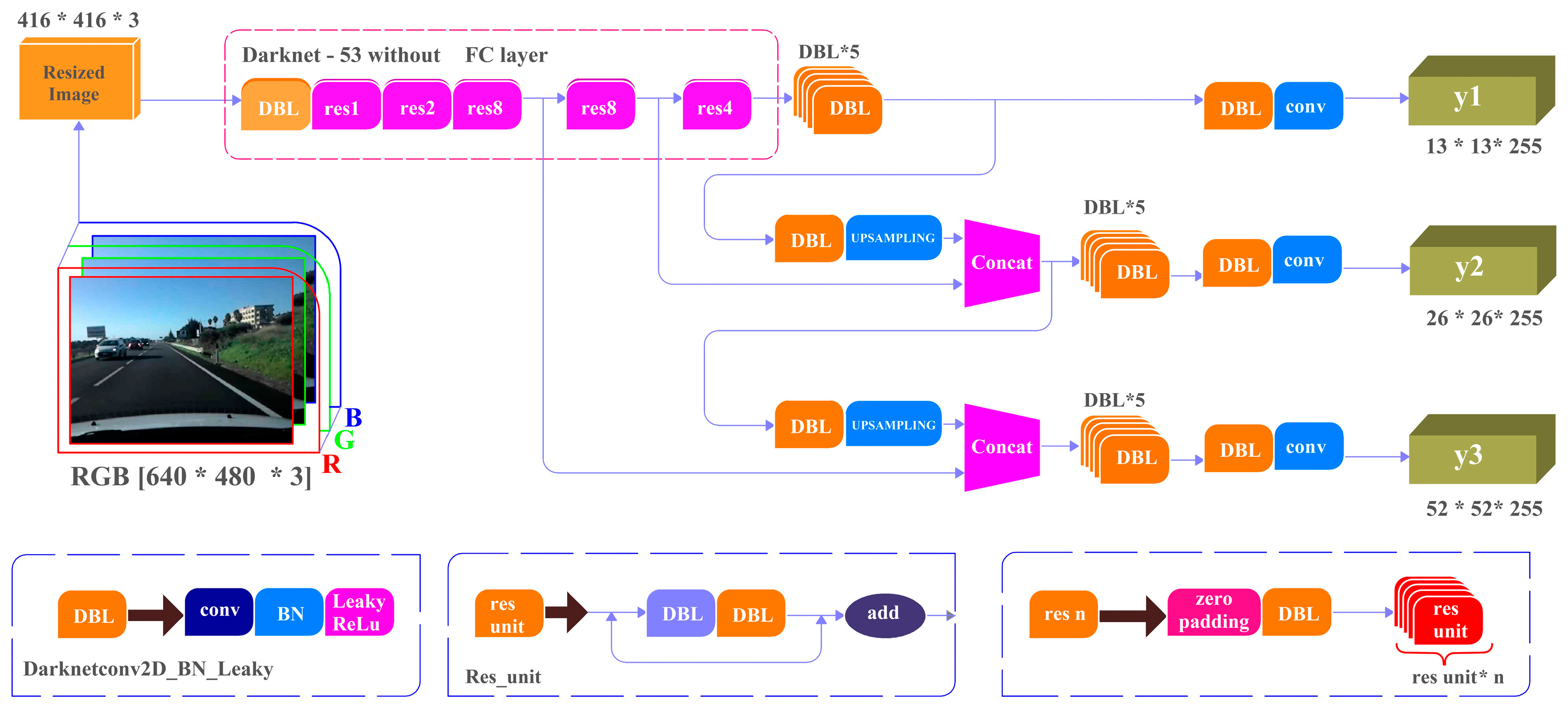
YOLOv3 is the latest version of YOLO and does not require a region proposal network (RPN) and directly performs regression to detect targets in the image [14]. In brief, YOLOv3 includes 53 convolutional layers and 23 residual layers as shown in Figure 1. YOLOv3 has shown significant advancement in real-time object detection, especially in the detection of smaller objects. Consequently, YOLOv3 is used for our vehicles detection system.

As explained in [14], 1 × 1, 3 × 3/2 and 3 × 3 convolution kernels of three sizes are applied in the convolutional layers to sequentially extract image features, ensuring the model has remarkable classification and detection performances. The remaining layers guarantee the convergence of the detection model [14].

In order to detect several areas of the same object at the same time, YOLOv3 fuses three feature maps of different scales (52 × 52, 26 × 26 and 13 × 13) by three time down sampling.

In this research, YOLOv3 is adopted because the YOLO family (i.e., YOLOv1, YOLOv2, YOLOv3) is a series of end-to-end deep learning models planned and designed for fast real-time object detection [9] and the quick vehicles detection is essential for the proposed MOM-DL technique.

Figure 1. YOLOv3 Network structure (adapted from [15]).

Figure 1. YOLOv3 Network structure (adapted from [15]).

2.2. YOLO V3 Algorithm

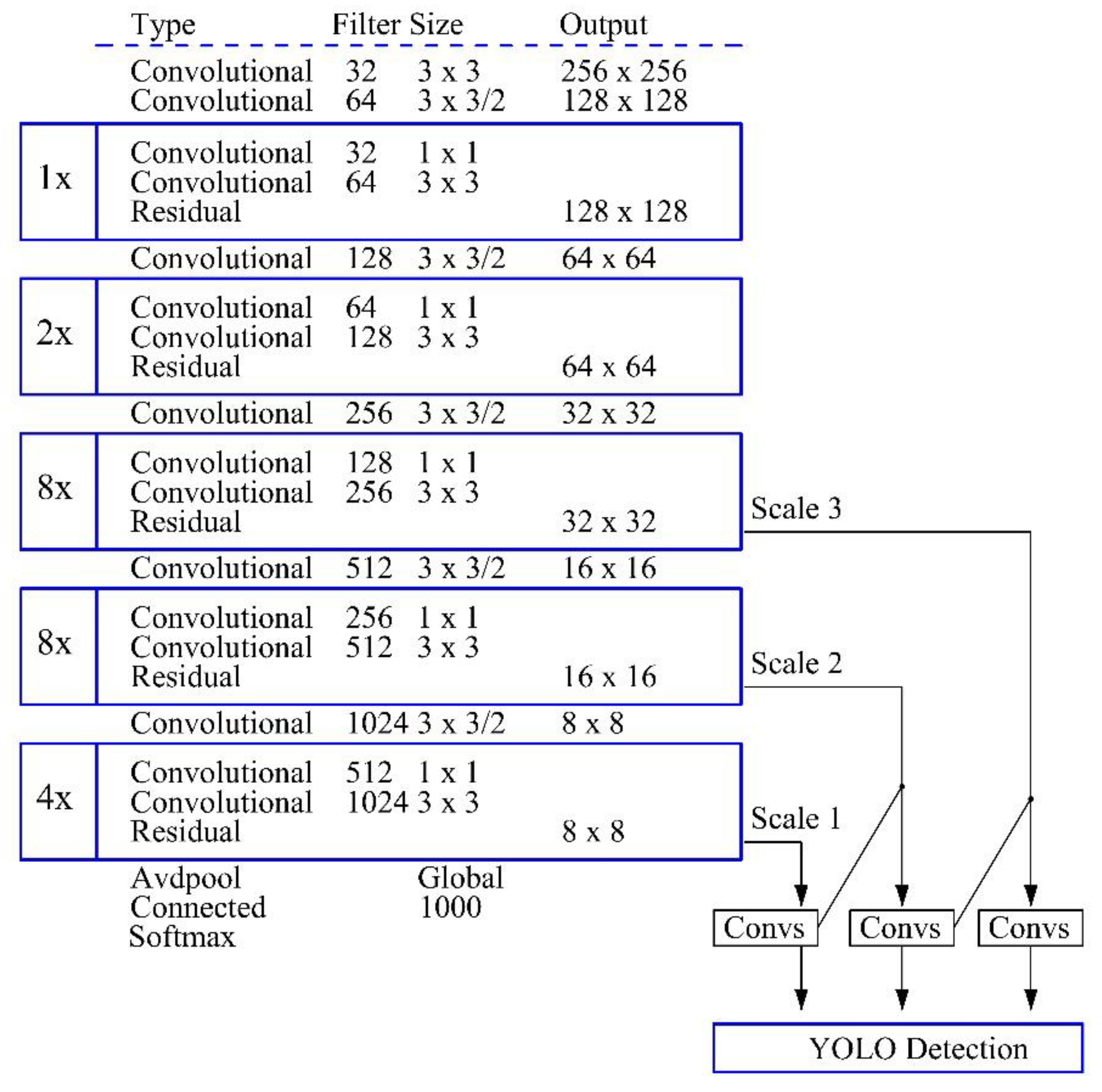
The network structure of YOLOv3 model uses the Darknet-53 network model that includes 5 residual modules and 53 convolutional layers (Figure 2).

As well explained in [16] the Darknet-53 network can “performed 5 down-sampling of the image, each of which has a sampling step size of 2 and a maximum step size of 32. Then the image is subjected to 32-fold down-sampling, 16-fold down-sampling, and 8-fold down-sampling processing to obtain 3 target detections with scale differences, Then the image is subjected to 32-fold down-sampling, 16-fold down-sampling, and 8-fold down-sampling processing to obtain 3 target detections with scale differences, the feature maps are respectively 13 × 13, 26 × 26, 52 × 52; The first feature map is suitable for detecting large targets, the second feature map tends to detect medium targets, and the last one is mostly used for small targets. Finally, the output feature map is sampled and feature fusion is performed, and finally the detection task of the target is completed”.

Figure 2. Darknet-53 structure diagram in YOLOv3 (adapted from [17]).

Figure 2. Darknet-53 structure diagram in YOLOv3 (adapted from [17]).

During the training process, the analyzed image is subdivided into S × S grids by the YOLOv3 model and each grid forecasts if the center of the object falls into its inner or not. In the first case, the grid predicts B detection bounding boxes and the Conf(Object) (i.e., the confidence of each box). In the second case, the candidate box confidence for the nonexistence of a target is imposed to zero. The previous conceptual and logical phases can be formalized with Equations (1)–(3) [9,18]:

$$\mathrm{C}\mathrm{o}\mathrm{n}\mathrm{f}(\mathrm{O}\mathrm{b}\mathrm{j}\mathrm{e}\mathrm{c}\mathrm{t})=\mathrm{Pr}(\mathrm{O}\mathrm{b}\mathrm{j}\mathrm{e}\mathrm{c}\mathrm{t})\times \mathrm{I}\mathrm{O}{\mathrm{U}}_{\mathrm{p}\mathrm{r}\mathrm{e}\mathrm{d}}^{\mathrm{t}\mathrm{r}\mathrm{u}\mathrm{t}\mathrm{h}}$$

(1)

$$\mathrm{Pr}(\mathrm{O}\mathrm{b}\mathrm{j}\mathrm{e}\mathrm{c}\mathrm{t})=\{\begin{array}{l}0 \mathrm{n}\mathrm{o} \mathrm{t}\arg \mathrm{e}\mathrm{t} \mathrm{i}\mathrm{n} \mathrm{t}\mathrm{h}\mathrm{e} \mathrm{c}\mathrm{e}\mathrm{l}\mathrm{l}\\ 1 \mathrm{t}\mathrm{h}\mathrm{e}\mathrm{r}\mathrm{e} \mathrm{a}\mathrm{r}\mathrm{e} \mathrm{t}\arg \mathrm{e}\mathrm{t}\mathrm{s} \mathrm{i}\mathrm{n} \mathrm{t}\mathrm{h}\mathrm{e} \mathrm{c}\mathrm{e}\mathrm{l}\mathrm{l}\end{array}$$

(2)

$$\mathrm{I}\mathrm{o}{\mathrm{U}}_{\mathrm{p}\mathrm{r}\mathrm{e}\mathrm{d}}^{\mathrm{t}\mathrm{r}\mathrm{u}\mathrm{t}\mathrm{h}}=\frac{{\mathrm{B}}_{\mathrm{g}\mathrm{r}\mathrm{o}\mathrm{u}\mathrm{n}\mathrm{d}\mathrm{t}\mathrm{r}\mathrm{u}\mathrm{t}\mathrm{h}}\cap {\mathrm{B}}_{\mathrm{p}\mathrm{r}\mathrm{e}\mathrm{d}\mathrm{i}\mathrm{c}\mathrm{t}\mathrm{e}\mathrm{d}}}{{\mathrm{B}}_{\mathrm{g}\mathrm{r}\mathrm{o}\mathrm{u}\mathrm{n}\mathrm{d}\mathrm{t}\mathrm{r}\mathrm{u}\mathrm{t}\mathrm{h}}\cup {\mathrm{B}}_{\mathrm{p}\mathrm{r}\mathrm{e}\mathrm{d}\mathrm{i}\mathrm{c}\mathrm{t}\mathrm{e}\mathrm{d}}}$$

(3)

where Conf(Object) is the confidence of the candidate box corresponding to the cell and $\mathrm{Io}{\mathrm{U}}_{\mathrm{pred}}^{\mathrm{truth}}$ is the intersection over union (ratio of the intersection area of the prediction box to the actual frame and the area of the union).

The $\mathrm{Io}{\mathrm{U}}_{\mathrm{pred}}^{\mathrm{truth}}$ measure evaluates the overlap between two bounding boxes: the ground truth bounding box (B_{ground truth}), that is, the hand-labeled bounding box created during the labeling process and the predicted bounding box (B_predicted) from the considered and proposed model. Each detected bounding box comprises the following parameters:

-

(x, y): position of the center of the detection bounding box relative to its parent grid;

-

(w, h) height and width of the detection bounding box;

-

Pr(Class_i|Object) probability of C categories: is the probability that the center of the i-th object falls into the grid.

Lastly, a tensor of the S × S (B × 5 + C) dimension is calculated.

2.3. Loss Calculation

YOLO predicts multiple bounding boxes per grid cell. To compute the loss for the true positive, it is required that one of them is responsible for the object. Therefore, we selected the one with the highest IoU (intersection over union) with the ground truth.

For calculation of loss, in YOLO, the sum-squared error between the predictions and the ground truth is used. The loss function comprises the classification loss, the localization loss (errors between the predicted boundary box and the ground truth) and the confidence loss (the objectness of the box) [19] as follows:

-

Classification loss: if an object is detected, the classification loss at each cell is the squared error of the class conditional probabilities for each class [19]:

$${\displaystyle \sum _{\mathrm{i}=0}^{{\mathrm{S}}^2}{\mathrm{I}}_{\mathrm{i}\mathrm{j}}^{\mathrm{o}\mathrm{b}\mathrm{j}}{({\mathrm{p}}_{\mathrm{i}}(\mathrm{c})-{\widehat{\mathrm{p}}}_{\mathrm{i}}(\mathrm{c}))}^2}$$

(4)

where:

${\mathrm{I}}_{\mathrm{i}\mathrm{j}}^{\mathrm{o}\mathrm{b}\mathrm{j}}$ = 1 if an object appears in the cell I, otherwise is 0;

${\widehat{\mathrm{p}}}_{\mathrm{i}}(\mathrm{c})$ the conditional class probability for class c in cell i.

-

Localization loss: evaluates the errors in the predicted boundary box locations and sizes. It is only counted the box responsible for detecting the object [19].

$${\mathsf{\lambda }}_{\mathrm{c}\mathrm{o}\mathrm{o}\mathrm{r}\mathrm{d}}{\displaystyle \sum _{\mathrm{i}=0}^{{\mathrm{S}}^2}{\displaystyle \sum _{\mathrm{j}=\mathrm{o}}^{\mathrm{B}}{\mathrm{I}}_{\mathrm{i}\mathrm{j}}^{\mathrm{o}\mathrm{b}\mathrm{j}}}}[{(\mathrm{x}-{\widehat{\mathrm{x}}}_{\mathrm{i}})}^2+{(\mathrm{y}-{\widehat{\mathrm{y}}}_{\mathrm{i}})}^2]+{\mathsf{\lambda }}_{\mathrm{c}\mathrm{o}\mathrm{o}\mathrm{r}\mathrm{d}}{\displaystyle \sum _{\mathrm{i}=0}^{{\mathrm{S}}^2}{\displaystyle \sum _{\mathrm{j}=\mathrm{o}}^{\mathrm{B}}{\mathrm{I}}_{\mathrm{i}\mathrm{j}}^{\mathrm{o}\mathrm{b}\mathrm{j}}}}{[{(\sqrt{{\mathsf{\varpi }}_{\mathrm{i}}}-\sqrt{{\widehat{\mathsf{\varpi }}}_{\mathrm{i}}})}^2+\sqrt{{\mathrm{h}}_{\mathrm{i}}}-\sqrt{{\widehat{\mathrm{h}}}_{\mathrm{i}}})}^2]$$

(5)

where:

${\mathrm{I}}_{\mathrm{i}\mathrm{j}}^{\mathrm{o}\mathrm{b}\mathrm{j}}$ = 1 if in the jth boundary box in cell i is responsible for detecting the object, otherwise 0;

${\mathsf{\lambda }}_{\mathrm{c}\mathrm{o}\mathrm{o}\mathrm{r}\mathrm{d}}$ increase the weight for the loss in the boundary box coordinates.

Confidence loss: if an object is detected in the box, the confidence loss (measuring the objectness of the box) is [19]

$${\displaystyle \sum _{\mathrm{i}=0}^{{\mathrm{S}}^2}{\displaystyle \sum _{\mathrm{j}=\mathrm{o}}^{\mathrm{B}}{\mathrm{I}}_{\mathrm{i}\mathrm{j}}^{\mathrm{o}\mathrm{b}\mathrm{j}}}}{(\mathrm{C}-{\widehat{\mathrm{C}}}_{\mathrm{i}})}^2$$

(6)

where:

${\widehat{\mathrm{C}}}_{\mathrm{i}}$ stands for the box confidence score of the box j, in the cell I;

${\mathrm{I}}_{\mathrm{i}\mathrm{j}}^{\mathrm{o}\mathrm{b}\mathrm{j}}$ = 1 if the jth boundary box in the cell i is responsible for detecting the object, otherwise 0.

If an object is not detected in the box, the confidence loss is [19]

$${\mathsf{\lambda }}_{\mathrm{n}\mathrm{o}\mathrm{o}\mathrm{b}\mathrm{j}}{\displaystyle \sum _{\mathrm{i}=0}^{{\mathrm{S}}^2}{\displaystyle \sum _{\mathrm{j}=\mathrm{o}}^{\mathrm{B}}{\mathrm{I}}_{\mathrm{i}\mathrm{j}}^{\mathrm{n}\mathrm{o}\mathrm{o}\mathrm{b}\mathrm{j}}}}{(\mathrm{C}-{\widehat{\mathrm{C}}}_{\mathrm{i}})}^2$$

(7)

where

${\mathsf{\lambda }}_{\mathrm{n}\mathrm{o}\mathrm{o}\mathrm{b}\mathrm{j}}$ is the complement of ${\mathrm{I}}_{\mathrm{i}\mathrm{j}}^{\mathrm{o}\mathrm{b}\mathrm{j}}$;

${\widehat{\mathrm{C}}}_{\mathrm{i}}$ is the box confidence score of the box j in the cell i;

${\mathsf{\lambda }}_{\mathrm{n}\mathrm{o}\mathrm{o}\mathrm{b}\mathrm{j}}$ weights down the loss when detecting background.

The final loss adds localization, confidence and classification losses together [19], as follows:

$$\begin{array}{l}{\mathsf{\lambda }}_{\mathrm{c}\mathrm{o}\mathrm{o}\mathrm{r}\mathrm{d}}{\displaystyle \sum _{\mathrm{i}=0}^{{\mathrm{S}}^2}{\displaystyle \sum _{\mathrm{j}=\mathrm{o}}^{\mathrm{B}}{\mathrm{I}}_{\mathrm{i}\mathrm{j}}^{\mathrm{o}\mathrm{b}\mathrm{j}}}}[{(\mathrm{x}-{\widehat{\mathrm{x}}}_{\mathrm{i}})}^2+{(\mathrm{y}-{\widehat{\mathrm{y}}}_{\mathrm{i}})}^2]+{\mathsf{\lambda }}_{\mathrm{c}\mathrm{o}\mathrm{o}\mathrm{r}\mathrm{d}}{\displaystyle \sum _{\mathrm{i}=0}^{{\mathrm{S}}^2}{\displaystyle \sum _{\mathrm{j}=\mathrm{o}}^{\mathrm{B}}{\mathrm{I}}_{\mathrm{i}\mathrm{j}}^{\mathrm{o}\mathrm{b}\mathrm{j}}}}{[{(\sqrt{{\mathsf{\varpi }}_{\mathrm{i}}}-\sqrt{{\widehat{\mathsf{\varpi }}}_{\mathrm{i}}})}^2+\sqrt{{\mathrm{h}}_{\mathrm{i}}}-\sqrt{{\widehat{\mathrm{h}}}_{\mathrm{i}}})}^2]+\\ {\displaystyle \sum _{\mathrm{i}=0}^{{\mathrm{S}}^2}{\displaystyle \sum _{\mathrm{j}=\mathrm{o}}^{\mathrm{B}}{\mathrm{I}}_{\mathrm{i}\mathrm{j}}^{\mathrm{o}\mathrm{b}\mathrm{j}}}}{(\mathrm{C}-{\widehat{\mathrm{C}}}_{\mathrm{i}})}^2+{\mathsf{\lambda }}_{\mathrm{n}\mathrm{o}\mathrm{o}\mathrm{b}\mathrm{j}}{\displaystyle \sum _{\mathrm{i}=0}^{{\mathrm{S}}^2}{\displaystyle \sum _{\mathrm{j}=\mathrm{o}}^{\mathrm{B}}{\mathrm{I}}_{\mathrm{i}\mathrm{j}}^{\mathrm{n}\mathrm{o}\mathrm{o}\mathrm{b}\mathrm{j}}}}[{(\mathrm{C}-{\widehat{\mathrm{C}}}_{\mathrm{i}})}^2+{\displaystyle \sum _{\mathrm{i}=0}^{{\mathrm{S}}^2}{\mathrm{I}}_{\mathrm{i}\mathrm{j}}^{\mathrm{o}\mathrm{b}\mathrm{j}}{({\mathrm{p}}_{\mathrm{i}}(\mathrm{c})-{\widehat{\mathrm{p}}}_{\mathrm{i}}(\mathrm{c}))}^2}\end{array}$$

(8)

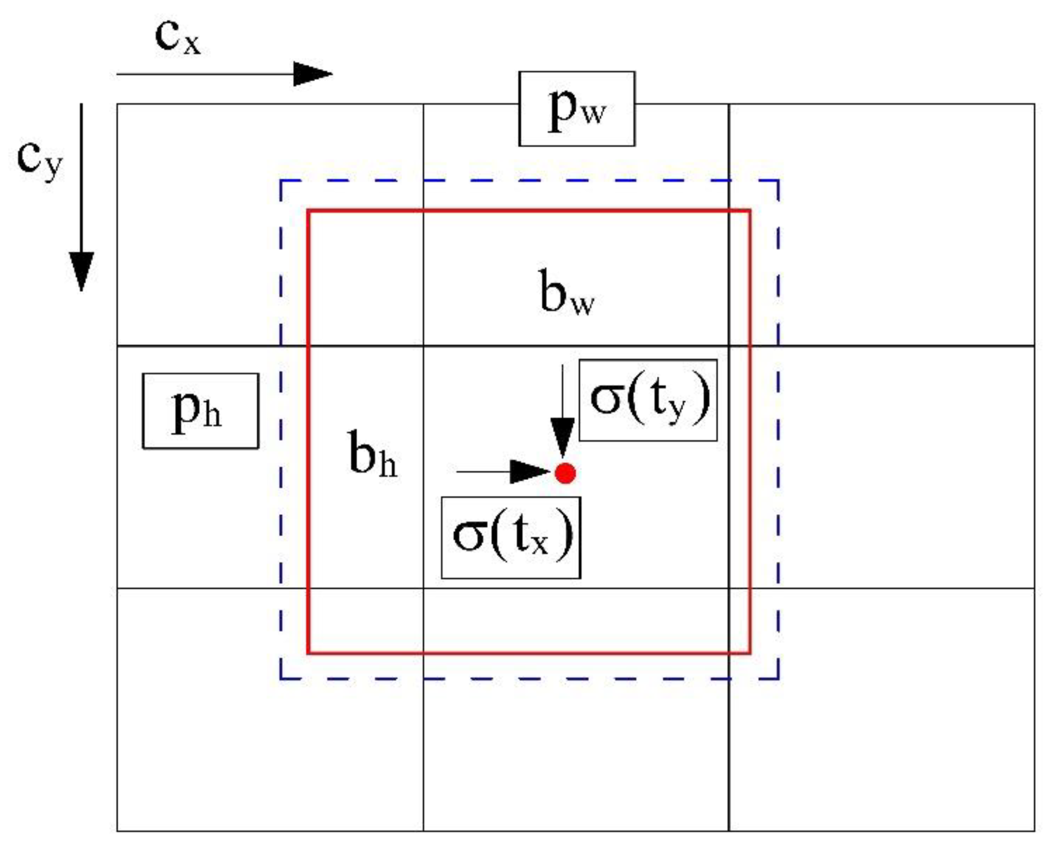
In YOLO v3, the method of predicting the bounding box (cfr. Figure 3) is given by Equation (9):

$$\{\begin{array}{l}{\mathrm{b}}_{\mathrm{x}}=\mathsf{\sigma }({\mathrm{t}}_{\mathrm{x}})+{\mathrm{c}}_{\mathrm{x}}\\ {\mathrm{b}}_{\mathrm{y}}=\mathsf{\sigma }({\mathrm{t}}_{\mathrm{y}})+{\mathrm{c}}_{\mathrm{y}}\\ {\mathrm{b}}_{\mathrm{w}}={\mathrm{p}}_{\mathrm{w}}{\mathrm{e}}^{{}_{{\mathrm{t}}_{\mathrm{w}}}}\\ {\mathrm{b}}_{\mathrm{h}}={\mathrm{p}}_{\mathrm{h}}{\mathrm{e}}^{{}_{{\mathrm{t}}_{\mathrm{h}}}}\end{array}$$

(9)

where t_x, t_y, t_w and t_h are the predicted outputs of the model, which represent the relative position coordinates of the center of the bounding box and the relative width and height of the bounding box. c_x and c_y represent the net, and p_w and p_h are the width and height of the predicted front bounding box. Finally b_x, b_y, b_w and b_h are the true coordinates of the center of the bounding box and the true width and height of the bounding box obtained after prediction.

The performance of a certain object detector can be measured mainly by the following metrics [20]:

-

Average mean precision (mAP) that is the integral over the precision p(o):

$$\mathrm{m}\mathrm{A}\mathrm{P}={\displaystyle \underset{0}{\overset{1}{\int }}\mathrm{p}(\mathrm{o})\mathrm{d}\mathrm{o}}$$

(10)

where p(o) is the precision of the object detection.

-

Frame per second (FPS) to measure detection speed (number of images processed every second);

-

Precision-recall curve (PR curve) in which Precision and Recall are calculated as follows:

$$\mathrm{R}\mathrm{e}\mathrm{c}\mathrm{a}\mathrm{l}\mathrm{l}=\frac{\mathrm{T}\mathrm{P}}{\mathrm{T}\mathrm{P}+\mathrm{F}\mathrm{N}}$$

(11)

$$\mathrm{Pr}\mathrm{e}\mathrm{c}\mathrm{i}\mathrm{s}\mathrm{i}\mathrm{o}\mathrm{n}=\frac{\mathrm{T}\mathrm{P}}{\mathrm{T}\mathrm{P}+\mathrm{F}\mathrm{P}}$$

(12)

-

Accuracy:

$$\mathrm{A}\mathrm{c}\mathrm{c}\mathrm{u}\mathrm{r}\mathrm{a}\mathrm{c}\mathrm{y}=\frac{\mathrm{T}\mathrm{P}+\mathrm{T}\mathrm{N}}{\mathrm{T}\mathrm{P}+\mathrm{T}\mathrm{N}+\mathrm{F}\mathrm{P}+\mathrm{F}\mathrm{N}}$$

(13)

The symbols TP, FN and FP stand for True Positive, False Negative and False Positive respectively.

-

Another parameter frequently used is the F1-score that is the harmonic mean of the precision and recall values:

$$\mathrm{F}1=\frac{2}{\frac{1}{\mathrm{p}\mathrm{r}\mathrm{e}\mathrm{c}\mathrm{i}\mathrm{s}\mathrm{i}\mathrm{o}\mathrm{n}}+\frac{1}{\mathrm{r}\mathrm{e}\mathrm{c}\mathrm{a}\mathrm{l}\mathrm{l}}}=\frac{2\mathrm{T}\mathrm{P}}{2\mathrm{T}\mathrm{P}+\mathrm{F}\mathrm{P}+\mathrm{F}\mathrm{N}}$$

(14)

F1-score can assume values in the range [0, 1]: if F1-score = 1 it results a perfect classifier. With reference to the semantic segmentation of images, F1-score indicates the proximity between the traced contour and the segmented contour.

3. Automatic Traffic Data Measurement Using Moving Observer Method

The moving observer method (MOM) was developed by Wardrop and Charlesworth [6] for macroscopic traffic variables measurements. Both the space mean speed vs. flow rate q measurements are obtained simultaneously through this method. This method requires a survey vehicle that travels in both directions on the analyzed highway. This procedure needs numerous runs of a survey vehicle done traveling in the same direction and against the traffic stream of interest. For each run (i.e., experiment) the human observers in the survey vehicle measure several traffic parameters, including the number of opposing vehicles met, the number of vehicles that the test vehicle overtook, the number of vehicles overtaking the test vehicle, the test vehicle mean speed, the length and the travel time of the run [6,21].

Equations (15)–(17) are used to calculate both the space mean speed and traffic flow for one direction of travel. In addition, vehicle density k can be estimated with Equation (18).

$$\mathrm{q}=\frac{\mathrm{x}+\mathrm{y}}{({\mathrm{t}}_{\mathrm{a}}+{\mathrm{t}}_{\mathrm{w}})}$$

(15)

$${\mathrm{t}}_{\mathrm{s}}={\mathrm{t}}_{\mathrm{w}}-\frac{\mathrm{y}}{\mathrm{q}}$$

(16)

$${\mathrm{v}}_{\mathrm{s}}=\frac{\mathrm{L}}{{\mathrm{t}}_{\mathrm{s}}}$$

(17)

$$\mathrm{k}=\frac{\mathrm{q}}{{\mathrm{v}}_{\mathrm{s}}}$$

(18)

where:

-

q is the estimated traffic flow on the lane in the direction of interest;

-

v_s is the space mean speed in the direction of interest;

-

k is the vehicle density in the direction of interest;

-

x denotes the number of vehicles traveling in the direction of interest that are met by the survey vehicle while traveling in the opposite direction;

-

y is the net number of vehicles that overtake the survey vehicle while traveling in the direction of interest (overtake test car—overtaken by test car);

-

t_a is the travel time taken for the trip against the stream;

-

t_s indicates the estimate of mean travel time in the direction of interest;

-

t_w is the travel time of the test vehicle with the stream;

-

L is the length of the highway segment under analysis and corresponds to the distance traveled by the survey vehicle.

According to [6], traffic flow values estimated by MOM may result in a small degree of bias. Counting processes are not affected by small deviations in the speeds of the test of the observed vehicles. Furthermore, no significant differences were found between macroscopic traffic flow variables values estimated by MOM and fixed spot measurement. Nevertheless, systematic errors may occur if the test vehicle speed v_w and the space mean speed vs. of the traffic streams have very similar values [6]. In the case of one-way roads, the observer vehicle is required to travel along the segment of interest at least with two speed values [22,23,24]. In accordance with [25], in order to guarantee reliable results with the use of MOM the choice of survey highway segment should stick with the following basic conditions:

-

Homogeneity: homogeneous in geometric characteristics (horizontal and vertical alignment, lanes and shoulders width, etc.) throughout the whole segment of length L;

-

Intersections: there is no at-grade intersection within the highway segment or within at least 250 m of its endpoints;

-

Speed limits: no sub-segment contained within it, or within 250 m of its endpoints, any speed restriction respect to the legal speed limit;

-

Roadworks: there are no roadworks;

-

Length: the segment length should be in the range of 1–5 km.

The suggested method MOM-DL, based on Computer Vision and Deep learning, is able to automatically detect, track and count along the analyzed highway segment the vehicles identified with “x” and “y” previously defined and classify them into different categories (motorbikes, light vehicles, heavy vehicles, etc.). The process is subdivided into subsequent steps: Vehicle Detection, Vehicle Classification and Recognition, Labeling, Tracking, Counting process.

In the counting process, first, the traffic variables x and y, t_a and t_w are evaluated and, lastly, the flow (q), the space mean speed (v_s) and density (k) are obtained using Equations (15)–(18). It is worth underlining that in a given video frame sequence the bounding box perimeter and surface of each detected vehicle change continuously over the time instants. The growth over time of the bounding box perimeter and area represents a reduction in the space headways between the observed vehicle (i.e., leader vehicle) and the survey vehicle (i.e., follower vehicle). Obviously, after an overtaking maneuver, the bounding box of the observed vehicle disappears in the video frame sequence. Then it is possible to count the number “y” of vehicles that overtake the survey vehicle when it travels the highway in the same direction of the traffic stream that should be examined. Correspondingly, the number “x” of vehicles met by the test vehicle traveling the highway segment in the opposite direction to the traffic stream of interest may be automatically measured.

These counting processes were implemented in Matlab R2020b using YOLOv3 and were applied in a case study (cfr. Section 4). The first results demonstrate that the MOM-DL is very accurate though various false positives (FP) and false negatives (FN) can be found in the detection step. This is because the test vehicle, and in turn the video camera, is subject to vibrations [26] caused by road pavement surface irregularities (including holes, bumps, and uneven pavement edge), lighting reflections and adverse environmental conditions (rain, fog darkness, etc.).

4. Experiments

The proposed method was applied to a segment of the Italian two-lane single carriageway SS640 highway. The analyzed highway segment of length L (L = 1.1 km), is characterized by uninterrupted flow conditions. Furthermore, this segment satisfies the basic conditions explained in the previous Section 3 concerning the homogeneity, intersections, speed limits, roadworks and length. The endpoints of the segment are denoted by sections A and B (Figure 7).

In accordance with the moving observer method, the survey vehicle was driven several times in the same direction and in the opposite direction with respect to the traffic stream that was to be measured (flow q). The survey vehicle speed was prefixed in the range 60 ± 5 km/h depending on the traffic condition. In the year 2021, 35 round trips for each direction were performed in the analyzed highway segment.

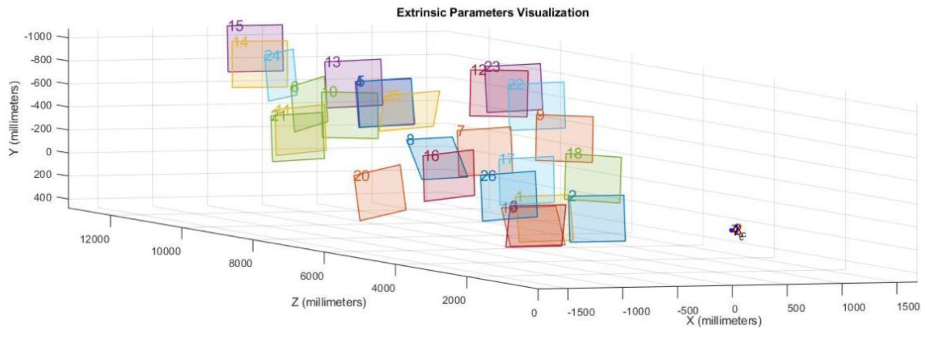
The videos of the traffic streams were recorded by a survey vehicle equipped with a calibrated camera (Figure 4). The first research phase was the camera calibration. Camera calibration aims at establishing two sets of parameters: intrinsic and extrinsic. The intrinsic parameters correct lens distortions while the extrinsic ones determine the spatial offset of the camera. The Zhang algorithm [27] determines the extrinsic parameters of the system. For the calibration processes, 64 different images were considered using a set of different photos as shown, for example, in Figure 5. Figure 6 shows the extrinsic parameter visualization obtained by the calibration processes. The calibrated model was then validated by several tests concerning the comparison between estimated and measured distances of the prefixed objects with respect to the camera lens. A similar technical approach can be applied in several fields of highway and transportation engineering [28,29].

By using Equations (15)–(18), for each run, the following parameters were estimated with the method MOM-DL:

-

The number y of vehicles that overtake the survey vehicle when it travels in the direction from A to B (see Figure 7 and Figure 12);

-

The number x of vehicles traveling in the direction of interest that are met by the survey vehicle while traveling in the opposite direction, from B to A (see Figure 7 and Figure 13);

-

The travel times t_a and t_w spent for crossing the segment in the two directions (from A to B and from B to A).

Figure 7. Analyzed segment of the highway SS 640.

Figure 7. Analyzed segment of the highway SS 640.

Training of the Neural Networks: Main Results

As explained in the previous Section 2.2 the Darknet-53 is a framework to train neural networks. Darknet-53 is open-source and is written in C and CUDA and serves as the basis for YOLOv3 [18].

Darknet-53 structure is summarized in Figure 2 [10,17]. In general, in Darknet-53, the weights of the custom detector are saved for every 100 until 1000 iterations, and it continues to be saved for every 10,000 iterations until it reaches the maximum batches [17]. A pre-existing vehicle dataset, consisting of 652 images published by [30,31,32] was used in this study. The pre-trained network can classify images into numerous object categories, such as cars, heavy vehicles, motorbikes, pedestrians, animals, etc. Also, an additional set of front images of private and public vehicles was added to the pre-existing vehicles dataset. The pre-existing vehicles dataset (including light and heavy vehicles, motorbikes, pedestrians and other users) in Darknet-53 was split into 70% for training and 30% for testing the neural networks.

As a result, the network learned feature-rich representations for a wide range of vehicle images. During the training process phase, data augmentation techniques (cropping, padding, flipping, etc.) were used in order to prepare the large neural networks. Then, a bounding box labeling tool [33] was applied to manually detect and recognize vehicles for the object to be detected [17]. Regarding the processing time of the training phase, consider, for example, the following parameters: 8 Epoch (1 Epoch = 25 iterations), learning rate = 0.001, L2 regularization factor = 0.0005, penalty threshold = 0.5, the result is a Time Elapsed = 00:40:20 h. The outcomes of this phase and the class label consist of four points of the position coordinate. The label was converted into YOLO format and the tool changed the values to a format that the training algorithm YOLOv3 can employ.

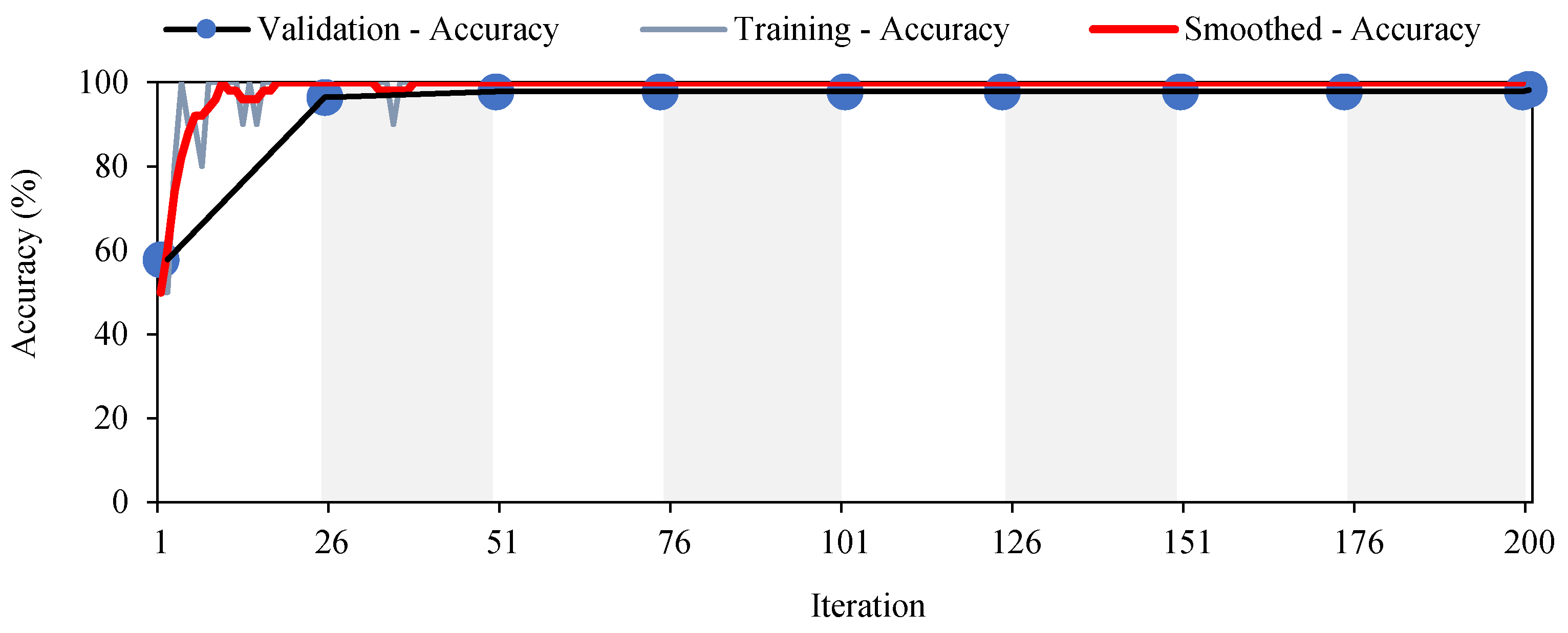
Figure 8 and Figure 9 show the training process consisting of 200 iterations. The Accuracy (Equation (13) and Figure 8), the Loss (Equation (8) and Figure 9) and the Precision (Equation (12) and Figure 10) values demonstrate that the proposed training model is able to detect the vehicles with high accuracy.

5. Results and Discussions

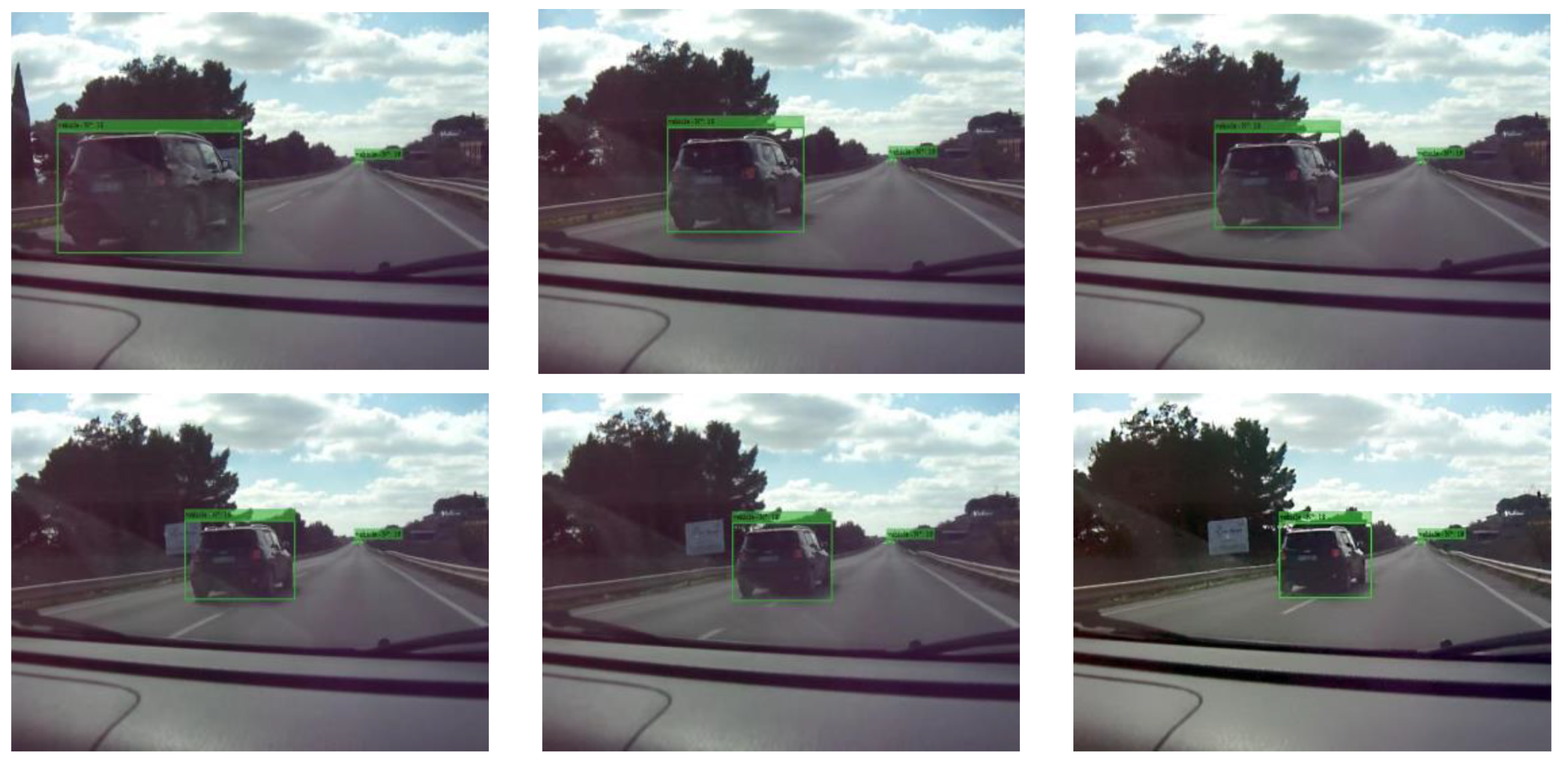
In computer vision, the tracking phase allows the detection of the same object (i.e., vehicle) in all its locations that may be identified in the consecutive frames of the recorded video. The phases employing the tracking algorithm are exemplified in Figure 11. During each test, in the sequence of video frames both the perimeter and surface of the bounding box relating to each vehicle changes over time. Therefore, the increase over time of this surface denotes the space headway decrease between the observed vehicle and the survey vehicle. Moreover, after an overtaking maneuver, the bounding box of the overtaken vehicle disappears [20,34]. Consequently, the traffic variable “y” (i.e., vehicles which overtaking the survey vehicle when it traveling the segment A-B, Figure 12) can be measured. Correspondingly, the number “x” of vehicles met by the survey vehicle while it was traveling in the opposite direction (i.e., against the traffic stream of flow q) was automatically measured, Figure 13. Then, for each of the thirty-five runs performed in the experiments, the macroscopic traffic variables (q; v_s; k) were automatically obtained by Equations (15)–(18).

Different vehicle types were detected [35] and homogenized to passenger car unit (pcu) by means of the HCM 2016 coefficients (flows were then expressed in pcu/h).

In order to estimate capacity, free-flow speed and other fundamental traffic variables, first the main traffic flow models v = v(k) were considered. Among these models, the bell-shaped curve model proposed by Drake, Schofer and May [36,37,38] (in short, the “May model” or “Drake model”) was adopted because it proved to be the best in interpreting the available experimental data. May’s equation, after logarithmic transformations, is as follows:

$$\ln (\mathrm{v})=\ln ({\mathrm{v}}_{\mathrm{f}})-\frac{{\mathrm{k}}^2}{2\cdot {\mathrm{k}}_{\mathrm{c}}{}^2}$$

(19)

or

V₁ = a + bD₁

(20)

in which V₁ = ln(v); a = ln (v_f); b = 1/(2 k_c²); D₁ = k². Where v_f denotes the free-flow speed and k_c the critical density, that is, the vehicle density associated with the capacity. By means of the fundamental flow relation q = k·v, it results in the following equations:

$$\mathrm{q}=\mathrm{v}\cdot \sqrt{\frac{\ln \frac{{\mathrm{v}}_{\mathrm{f}}}{\mathrm{v}}}{\frac{0.5}{{\mathrm{k}}_{\mathrm{c}}^{}{}^2}}}$$

(21)

$$\mathrm{q}={\mathrm{v}}_{\mathrm{f}}\cdot \mathrm{k}\cdot {\mathrm{e}}^{-\frac{1}{2}{\left(\frac{\mathrm{k}}{\mathrm{k}\mathrm{c}}\right)}^2}$$

(22)

which allow the two additional flow relations to be traced: vs. = vs. (q) and q = q(k). Finally, the flow models were calibrated. By observing Equations (21) and (22), it can be realized that the two parameters needed to be assessed are the free-flow speed v_f and the critical density k_c.

On the basis of scatter plots (k; ln(v_s)) the model calibration parameters v_f and k_c were deducted as shown in Figure 14 for both traffic data acquirement methods (i.e., MOM and MOM-DL). For instance, in the case of MOM-DL method, the Figure 14b shows the speed –density scatter points (k; ln(v_s)). In this case, it results: v_f = exp(a) = exp(4.2745) = 71.84 km/h; ${\mathrm{k}}_{\mathrm{c}}=\sqrt{\frac{1}{-2\cdot \mathrm{b}}}=\sqrt{\frac{1}{-2\cdot (-0.0006)}}$ = 28.87 pcu/km/lane. Therefore, the calibrated relation q = q(k) is: $\mathrm{q}=71.84\cdot \mathrm{k}\cdot {\mathrm{e}}^{-\frac{1}{2}{\left(\frac{\mathrm{k}}{28.87}\right)}^2}$.

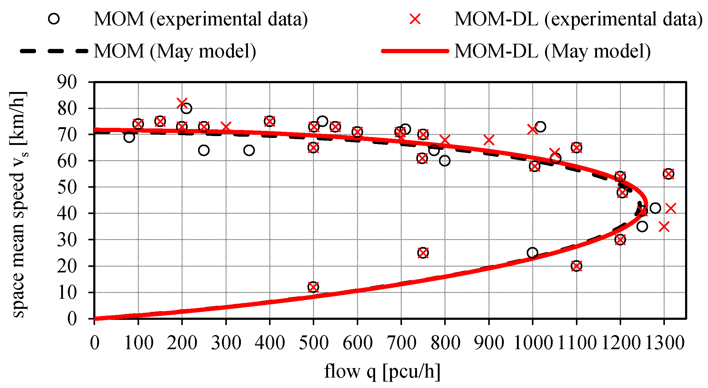
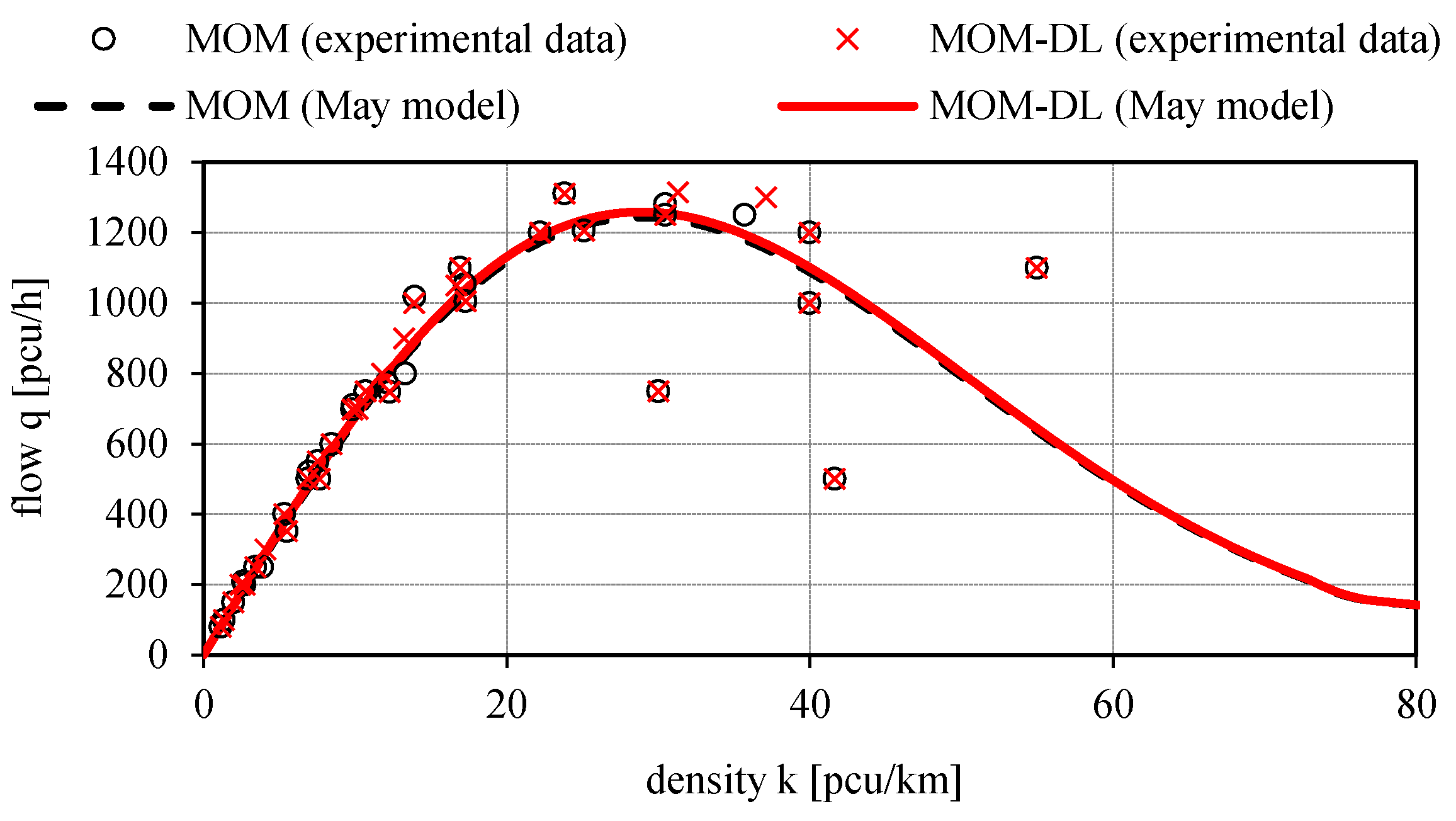
Figure 15, Figure 16 and Figure 17 illustrate the calibrated May’s traffic relationships v_s = v_s(q), v_s = v_s(k), q = q(k) with the overlapping of the values of the experimental traffic variables measured by the proposed automated counting method based on deep learning (MOM-DL) in comparison with those measured by the conventional one (MOM). The two methods are in good agreement with each other but with the MOM-DL method, as stated above, some false positives (FP) and false negatives (FN) can be found in the detection step because of camera vibrations or adverse environmental conditions. In any case, it can be noted that the values of the traffic variables estimated with the proposed method (MOM-DL) are close to those of the traditional one (MOM). As a matter of fact, with respect to MOM, the MOM-DL technique can lead to lower values of some traffic flow variables such as the free-flow speed v_f, the capacity c, the critical speed v_c, and the critical density k_c, though the maximum percentage variation is relatively modest (2.3%, as shown in

Table 2. Comparison among the values of the traffic flow variables obtained with MOM-DL and MOM methods.

Method	Free-Flow Speed vf [km/h]	Lane Capacity c [pcu/h]	Critical Speed vc [km/h]	Critical Density kc [pcu/km]
MOM	71.06	1244.15	43.00	28.87
MOM-DL	71.84	1257.80	44.00	28.87
Δ [%]	1.1	1.1	2.3	0.0

).

6. Conclusions

The evaluation of traffic flow variables is a key element in highway planning and design phases, as well as in traffic control strategies of existing infrastructures. Traffic data can be collected by numerous techniques, including the fixed spot measurement and the “probe vehicle data” systems. In addition, the moving observer method (MOM) developed by Wardrop can be used as a traffic data acquirement method. As is well known, artificial intelligence (AI) and deep learning (DL) are commonly used in numerous applications of real-life areas including vehicle detection and recognition.

This article presents a novel automatic traffic data acquirement system founded on MOM, deep learning and the YOLOv3 algorithm for the estimation of macroscopic traffic variables. The proposed method, called MOM-DL, allows the measurement of the flow rate (q), the space mean speed (v_s) and the density (k) in case of stationary and homogeneous traffic flow conditions. Being an automated method, MOM-DL does not necessitate human observers with consequent significant advantages in terms of user safety improvements and costs reductions. MOM-DL was subjected to strong verification, calibration and validation by means of real-world traffic datasets. Experiments have been conducted along a segment of an Italian highway (SS640) having a length of 1.1 km and uninterrupted flow conditions.

In accordance with the moving observer method, the survey vehicle has been driven numerous times in the same direction and in the opposite direction with respect to the traffic stream of flow q that must be measured. The test vehicle speed has been fixed in the range 60 ± 5 km/h depending on the traffic state condition. For each of the 35 trips, the vehicles belonging to the flow of interest have been recorded by means of a calibrated video camera installed in the survey vehicle.

The accuracy, loss and precision values obtained during the neural network training process prove that the proposed training model detects vehicles with high accuracy. The traffic flow variables have been calculated using the Wardrop relationships q = q(x, y, t_a, t_w), vs. = v_s(x, y, t_a, t_w), k = k (x, y, t_a, t_w). Then, the empirical traffic data, in terms of pairs (q; v_s), (k; v_s), (k; q) were employed for the comparison between MOM-DL and MOM. The results of the research demonstrate that the two methods are in good agreement with each other, although some false positives and false negatives may be found in the detection step mainly due to camera vibrations.

The proposed method is marked by a reliable and rapid analytical approach as well as by high accuracy in the measurements of traffic variables. In fact, the research shows that the values of the macroscopic traffic variables estimated by means of the May traffic flow model together with the proposed method (MOM-DL technique) are very close to those obtained by the traditional one (MOM technique), with the maximum percentage variation being less than 3%.