Article

BAT Algorithm-Based ANN to Predict the Compressive Strength of Concrete—A Comparative Study

by
Nasrin Aalimahmoody
1,
Chiara Bedon
2,*,
Nasim Hasanzadeh-Inanlou
3,
Amir Hasanzade-Inallu
4 and
Mehdi Nikoo
5
1
Department of Electrical Engineering, Yazd Branch, Islamic Azad University, 89158-13135 Yazd, Iran
2
Department of Engineering and Architecture, University of Trieste, 34127 Trieste, Italy
3
Department of Industrial and Mechanical Engineering, Qazvin Branch, Islamic Azad University, 34185-1416 Qazvin, Iran
4
Department of Earthquake Engineering, Science and Research Branch, Islamic Azad University, 15847-43311 Tehran, Iran
5
Young Researchers and Elite Club, Ahvaz Branch, Islamic Azad University, 61349-37333 Ahvaz, Iran
*
Author to whom correspondence should be addressed.
Infrastructures 2021, 6(6), 80; https://doi.org/10.3390/infrastructures6060080
Submission received: 1 May 2021 / Revised: 21 May 2021 / Accepted: 23 May 2021 / Published: 26 May 2021
(This article belongs to the Special Issue Sustainability of Building Materials and Structures)

Abstract

:
The number of effective factors and their nonlinear behaviour—mainly the nonlinear effect of the factors on concrete properties—has led researchers to employ complex models such as artificial neural networks (ANNs). The compressive strength is certainly a prominent characteristic for design and analysis of concrete structures. In this paper, 1030 concrete samples from literature are considered to model accurately and efficiently the compressive strength. To this aim, a Feed-Forward (FF) neural network is employed to model the compressive strength based on eight different factors. More in detail, the parameters of the ANN are learned using the bat algorithm (BAT). The resulting optimized model is thus validated by comparative analyses towards ANNs optimized with a genetic algorithm (GA) and Teaching-Learning-Based-Optimization (TLBO), as well as a multi-linear regression model, and four compressive strength models proposed in literature. The results indicate that the BAT-optimized ANN is more accurate in estimating the compressive strength of concrete.

1. Introduction

Civil engineers have always been interested in estimating the properties of concrete as a composite material by utilizing analytical models, as well as investigating the effect of each component of the mix design on its properties. The first step in all rehabilitation projects is to obtain information about the current conditions of the structure and its analysis. In this regard, using field experiments to perform this evaluation is very important. In these projects, destructive experiments are used to achieve more accurate results, which involve high costs and structure destruction [1]. The application of artificial neural networks and evolutionary optimization algorithms to determine concrete’s compressive strength has received a lot of attention in recent years [2].
Many studies on the use of artificial neural networks (ANNs) to assess the compressive strength of concrete (f’c) have been conducted in recent decades. Artificial neural network models have proved to be superior for the determination of concrete compressive strength in Alto Sulcis Thermal Power Station in Italy [3], in-place concrete strength estimation to facilitate concrete form removal and scheduling for construction [4], prediction of compressive strength of concrete subject to lasting sulfate attack [5], determination of low-, medium-, and high-strength concrete strength [6], accurate assessment of compressive strength of large-volume fly ash concrete [7], approximating compressive strength of concrete based on weight and ultrasonic pulse velocity [8], compressive strength prediction of high performance concrete [9], and compressive strength estimation of concrete containing various amounts of furnace slag and fly ash [10].
Artificial neural networks are also utilized in modelling high-strength concrete specimens due to the non-linearity of the parameters. Yeh [11,12] predicted high-performance concrete compressive strength using ANNs by performing a series of tests. Artificial neural networks have been more accurate than models based on regression analysis. Öztaş et al. [13] determined the compressive strength of high-strength concrete using ANNs and 187 samples for modelling. The parameters of cover, the water to binder ratio, water content, fine aggregate ratio, fly ash content, air-entraining agent, superplasticizer, and silica fume replacement were employed as input parameters. The results confirmed that an ANN could forecast the compressive strength of high-strength concretes satisfactorily.
Numerous articles have then been published on the use of optimization algorithms with ANNs. In [14], an ANN combined with the metaheuristic Krill Herd algorithm was used to provide satisfactory results in terms of estimation of the mechanical properties of alkali-activated mortar mixes (AAMs). Behnood et al. [15] estimated the compressive strength of silica fume concrete using an ANN as an optimization problem. To find a simple ANN model with acceptable error, they proposed a new multi-objective optimization method called the Multi-Objective Grey Wolves Optimization (MOGWO) method. Sensitivity analysis was also performed to evaluate the final ANN model’s ability to predict silica fume concrete compressive strength by changing the strength variables. Nazari et al. [16] determined the compressive strength of concrete using titanium dioxide (TiO2) nanoparticles. A genetic algorithm (GA) was used to adjust the weights of the network. The results showed that optimization increases the accuracy of the model. Bui et al. [17] considered the combination of ANNs with firefly algorithms to predict the compressive and tensile strength of high-performance concrete. The results indicate the high performance and accuracy of the proposed model. Sadowski et al. [18] used the colonial competition algorithm to determine the compressive strength of concrete. Their study considered the feasibility of using the algorithm to learn ANN parameters and compared the proposed model with the GA-based ANN. The results confirmed that the ANN combined with the colonial competition algorithm resulted in the least prediction error. Duan et al. [19] used the colonial competition algorithm to determine the compressive strength of recycled aggregate concrete. Zhou et al. [20] utilized ANNs and adaptive neuro-fuzzy inference systems to estimate the compressive strength of hollow concrete block masonry prisms. The analysis was based on 102 data points and showed that the proposed models have excellent prediction with negligible error rates. Armaghani et al. [21] developed neuro-fuzzy systems to predict concrete compressive strength.
The current study concentrates on boosting the accuracy of an ANN model by applying the BAT optimization algorithm. To this aim, the dataset has been collected from UCI (University California Irvine) machine learning repository which includes 1030 experimental results collected from peer-reviewed articles. Section 2 delivers the essential background on ANNs and the BAT algorithm. The experimental model establishment and training are described in Section 3. Section 4 presents detailed results and assesses the efficiency of the model based on comparative analyses.

2. Background

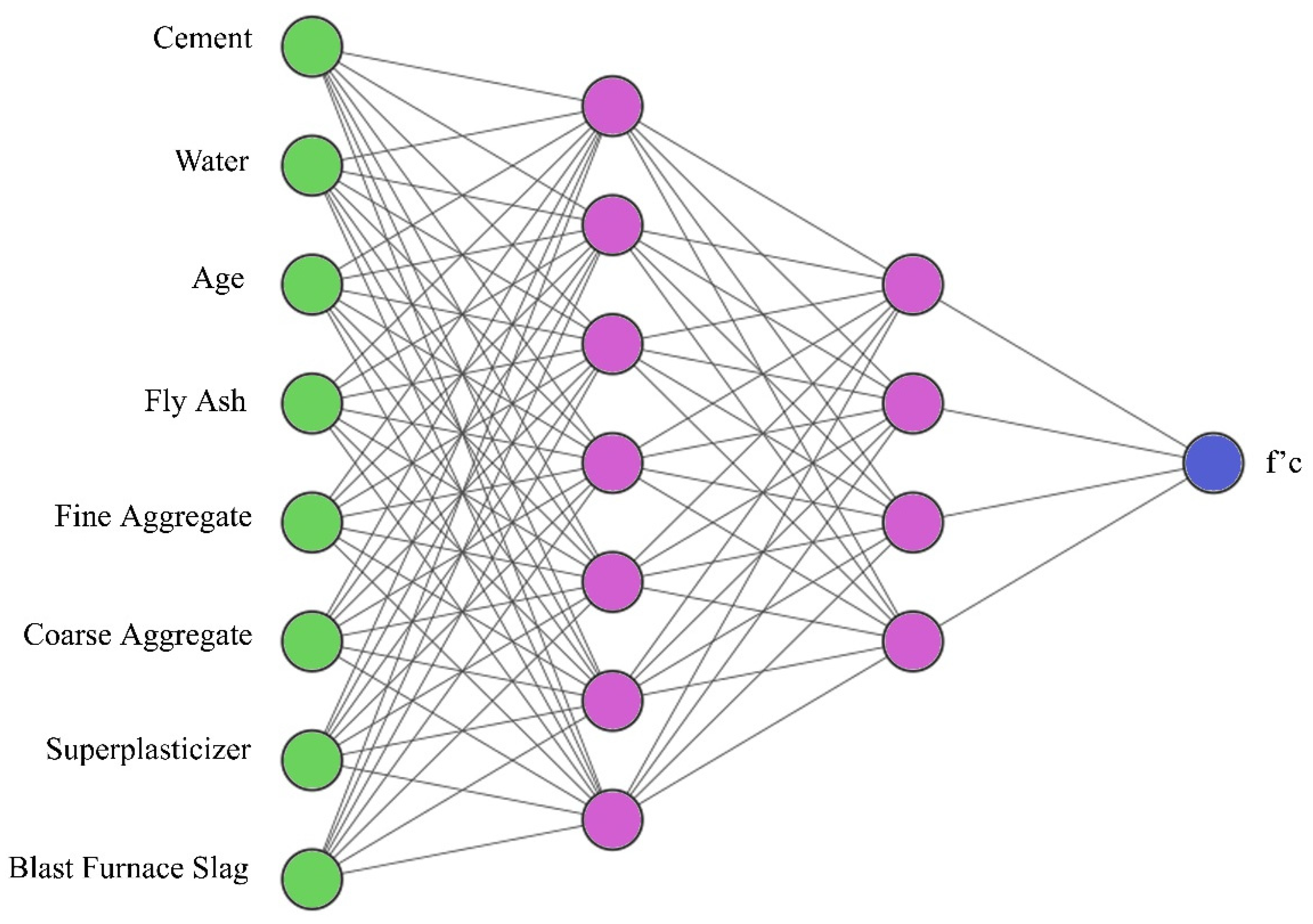
2.1. Artificial Neural Networks

Artificial neural networks, a form of data processing systems, are algorithms that simulate biological neurons’ function. ANNs improve their performance by learning from data in the training step [22,23]. The main assumptions of an artificial neural network model are as follows [24,25]:
  • Data are handled in specific entities called nodes.
  • Links relay signals between nodes.
  • The weight assigned to each link indicates the strength of that link.
  • Nodes calculate their outputs by applying activation functions to input data.
The Feed-Forward network is an ANN model in which the connections of its constituent units do not form a cycle. This network is different from a recurrent neural network, given that data move only in one direction, the direction of which is forward. Data initially starts from input nodes and passes through hidden layers to the output nodes [26]. Figure 1 shows an example of a feed-forward network. Typically, data in ANN are split into three distinct subgroups [23]:
  • Training: this subgroup of data is used to train the ANN, and learning occurs through examples, similar to the human brain. The training sessions are repeated until the acceptable precision of the model is achieved.
  • Validation: this subset determines the extent of training of the model and estimates model features such as classification errors, mean error for numerical predictions, etc.
  • Testing: This subgroup can confirm the performance of the training subset developed in the ANN model.

2.2. BAT Algorithm

By utilizing their sophisticated echolocation facilities, bats can avoid obstacles and detect prey. Utilizing the time interval between a pulse emission and its echo, they develop a three-dimensional depiction of their surrounding [27]. Inspired by this behaviour of bats, Yang [28] developed the BAT algorithm. In the algorithm idealization it is assumed that:
  • bats use echolocation, and they can discern between prey and surroundings;
  • at any given location xi, they fly randomly with velocity vi and contingent upon the location of prey they adjust their rate of pulse emission;
  • the loudness of the emitted pulse ranges from A0 to a minimum value of Amin.
Firstly, the BAT algorithm initializes a random population of bats, and then updates their frequencies using Equation (1) [29]:
f i = f m i n + ( f m a x f m i n ) β
where fi is the i-th bat frequency, fmin is the min frequency, fmax is the max frequency, and β is a random quantity between 0 and 1. The location and velocity of bats are revised according to:
V i t + 1 = V i t + ( x i t x * ) f i
x i t + 1 = x i t + V i t + 1
where V i t is the i-th bat velocity at recurrence t, xit is the i-th bat position at recurrence t, and x * is the global best position. Then, the procedure shifts some bats to a vicinity of the top global location as:
x n e w = x o l d + ε A t
where A denotes loudness and ε is a random quantity between 0 and 1. The criterion for accepting the new position of each bat is a cost value less than the previous iteration. The algorithm then revises the pulse rate and loudness using Equations (5) and (6):
A i t + 1 = α A i t
r i t + 1 = r i 0 ( 1 exp ( γ t ) )
where α is a constant typically selected between zero and one, r0i is the initial pulse rate and γ is a constant.
This algorithm can be utilized to train an ANN. In the present application, the weights and biases of the network are considered as the position vector of a bat, and therefore each bat represents a vector of weights of an artificial neural network. The cost function is the prediction error of the network. The final solution of the bat algorithm results in a trained network [29].

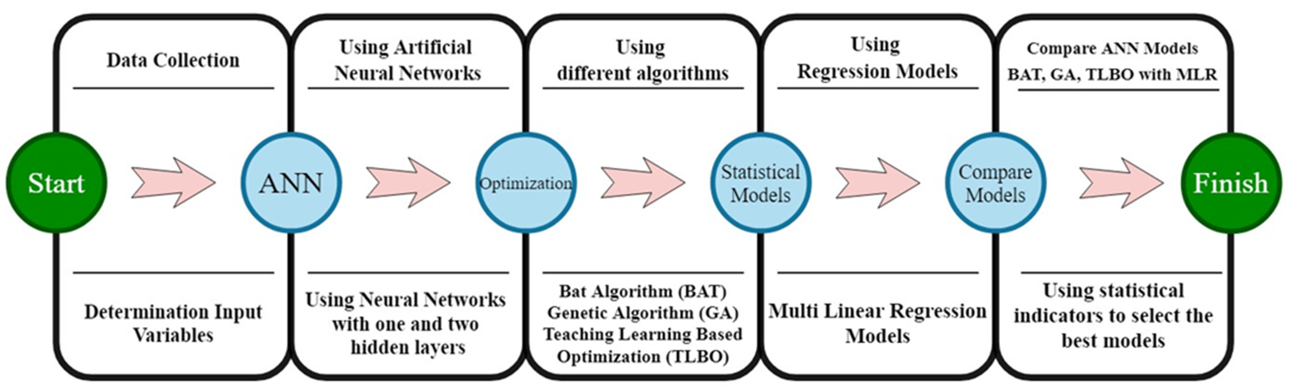
3. Methods and Materials
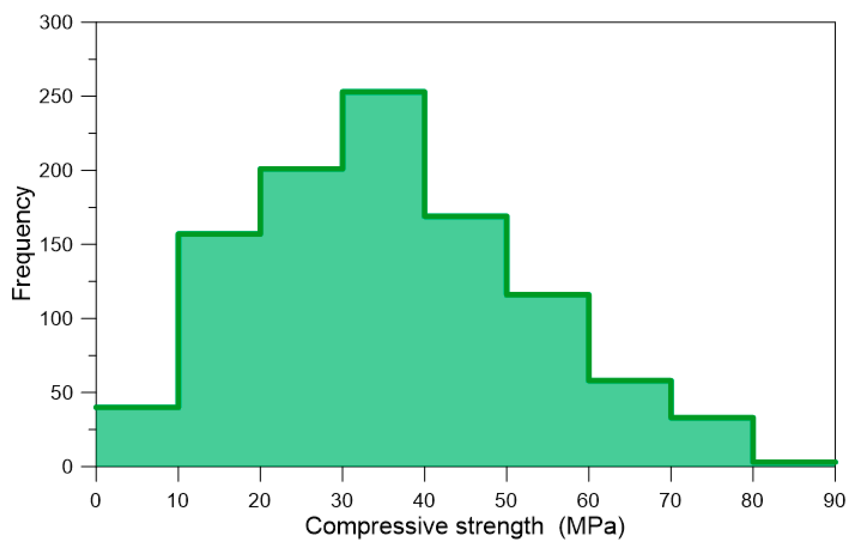
3.1. Dataset

The dataset utilized in this study was used to follow the schematic procedural steps proposed in Figure 2. More precisely, according to [12], it consists of 1030 concrete compressive strength test results from various sources. The influencing parameters on the concrete compressive strength are cement, blast furnace slag, fly ash, water, superplasticizer, coarse aggregate, and fine aggregate age. Table 1 gives the descriptive statistics of samples from [12]. The selected target value is the 28-day compressive strength of concrete.
Following Figure 3, where the histogram for the 28-day compressive strength for concrete specimens is proposed, it can be observed that 780 samples have compressive strength values ranging from 10 to 50 MPa.
If the ANN input variables have different ranges, the training process can suffer from adverse impacts, such as the optimization divergence of algorithm and increased training time [30]. Using Equation (7), each variable was hence normalized into the range from −1 to 1, that is [31]:
Y n = 2 ( Y Y m i n ) Y m a x Y m i x 1
where Y is the original value of the variable, Yn is the normalized value, Ymax is the max, and Ymin is its min value. Table 1 shows the minimum and maximum values and the target values of concrete compressive strength used for each of the eight input parameters. It is worth noting that the ANN will undergo training using the normalized data. Therefore, it is essential to feed the network with normalized variables when using the ANN to predict new values and un-normalize the data (i.e., transferring them into their original range, the network outputs).

3.2. Performance Measures

Statistical measures are employed to determine the model accuracy. Using the statistical index helps choose the best model with the least error and select the model with the most generalizability.
The statistical measures employed in evaluating the accuracy of different topologies are Mean Error (ME), Mean Absolute Error (MAE), Mean Squared Error (MSE), and Root Mean Squared Error (RMSE) [32]:
M E = 1 n i = 1 n ( P i O i )
M A E = 1 n i = 1 n | P i O i |
M S E = 1 n i = 1 n ( P i O i ) 2
R M S E = [ 1 n i = 1 n ( P i O i ) 2 ] 1 2
where P i and O i represent predicted and observational data, and n represents the number of cases.

3.3. Experimental Model Generation Utilizing ANNs and BAT Algorithm

Eight input factors, influencing the concrete compressive strength, are used in the suggested model. Thus, trained artificial neural networks have eight nodes in the input layer and one node in the output layer (Figure 2). Networks with one or two hidden layers have been used for modelling. A network can have a very high performance in the training phase but may not show the same accuracy in the testing phase. Hence, it is better to randomly bifurcate the data and with a suitable ratio for each stage [33]. To this end, the data were randomly split into two groups to reduce overfitting effects. For training, 70% of data (721 samples) were used and the remaining 30% (309 pieces) were used to test network performance. For an artificial neural network model, the number of hidden layers and the total number of nodes in the hidden layers depends on the problem [34]. Accordingly, trial-and-error was used to obtain the ideal topology (i.e., the topology that best represents the data). A common formula for the total number of nodes in an ANN is given in Equation (12) [35]:
N H 2 N I + 1
where N H   is the number of neurons in the hidden layer and N I   is the number of inputs to the network. Since there are eight factors, the equation indicates that the number of hidden layer nodes must be less than 17. Thus, different architectures have a maximum of two hidden layers and a maximum of 17 trained neurons. In mode one, the network hidden layer has a maximum of 17 neurons in the hidden layer. In mode two, the hidden layer has one to nine neurons. A total of 89 different architectures were selected for training. The topologies used are given in Table 2.
The tanh function was picked as the transfer function of the nodes in the hidden layer in all the ANNs. Meanwhile, the identity relation was selected as the transfer function of the nodes in the output layer. The bat algorithm was then used to refine the parameters of the artificial neural network to result in the least predictive error. The bat algorithm and ANNs were developed using MATLAB [36]. The hyperparameters of the bat algorithm used for training the 89 ANN topologies are given in Table 3.

4. Results

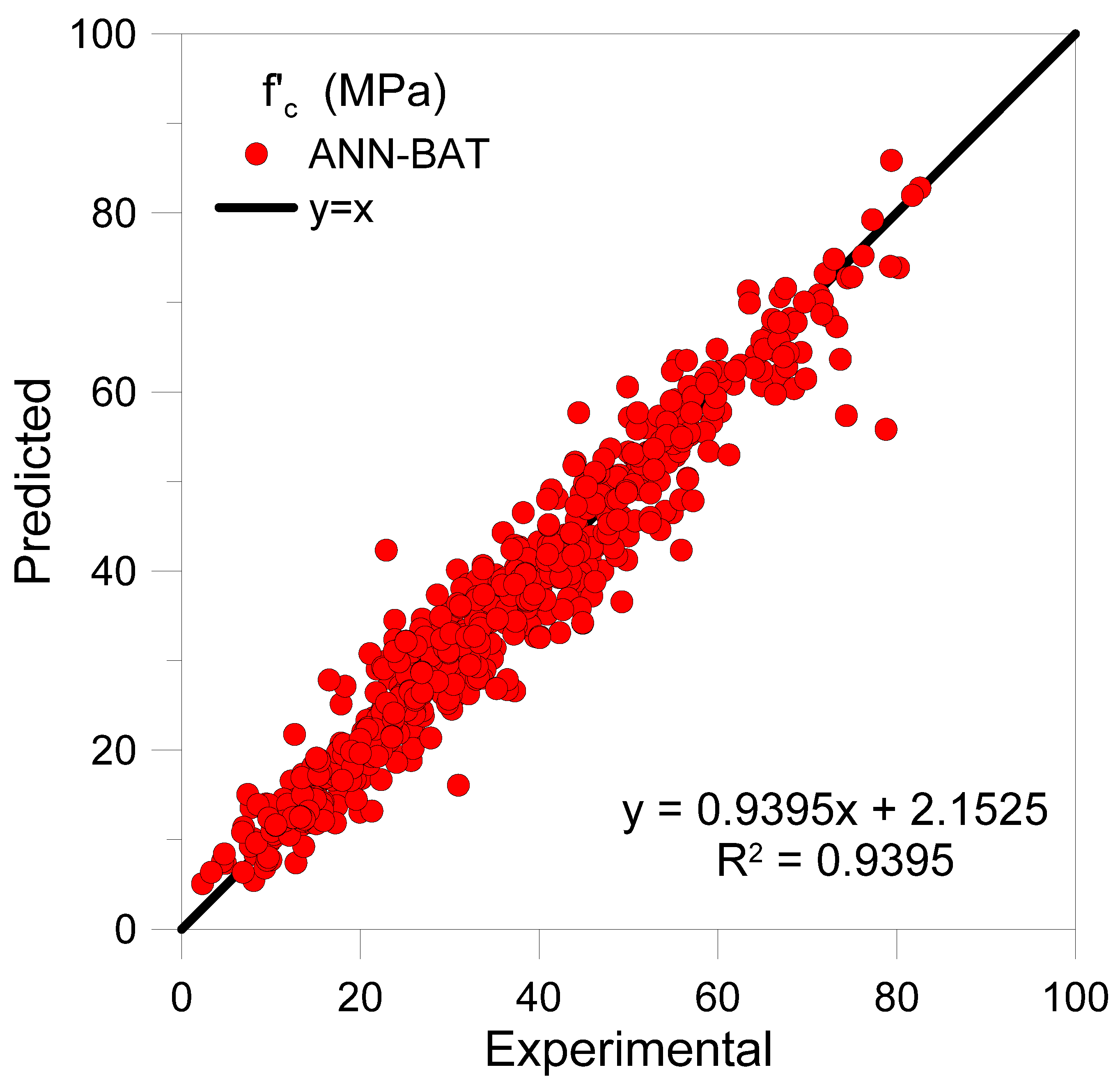
4.1. Experimental Model Assessment

The number of used models was set to 89. In addition, one-layer and two-layer artificial neural networks were used. The bat optimization algorithm is used to refine the weights of the network. The transfer function for all networks is the tanh function. Among the models trained to determine concrete compressive strength, four models were selected as the best models based on parameters presented in Section 3.2. The error metrics of these models in the training phase are given in Table 4. The test results of the models are given in Table 5.
According to Table 4 and Table 5, the ANN-BAT-2L (7-4) network has the lowest MSE, ME, MAE, and RMSE indices. For this network, the R 2 value in the training and testing phases is equal to 0.9395 and 0.9134, respectively, supporting the model’s high precision. The test phase values in MSE, ME, MAE, and RMSE indices are equal to 27.624, −0.664, 3.847 and 5.256, respectively, indicating high modelling precision in forecasting the concrete’s compressive strength. Error metrics for samples are given based on the original range of variables.
To visualize the accuracy of ANN-BAT-2L (7-4), the experimental model predicted values versus their values from the experiment are shown in Figure 4 and Figure 5 for the train and test data, respectively. The predictions of the network are near the identity function values, which suggests that the network is highly accurate.

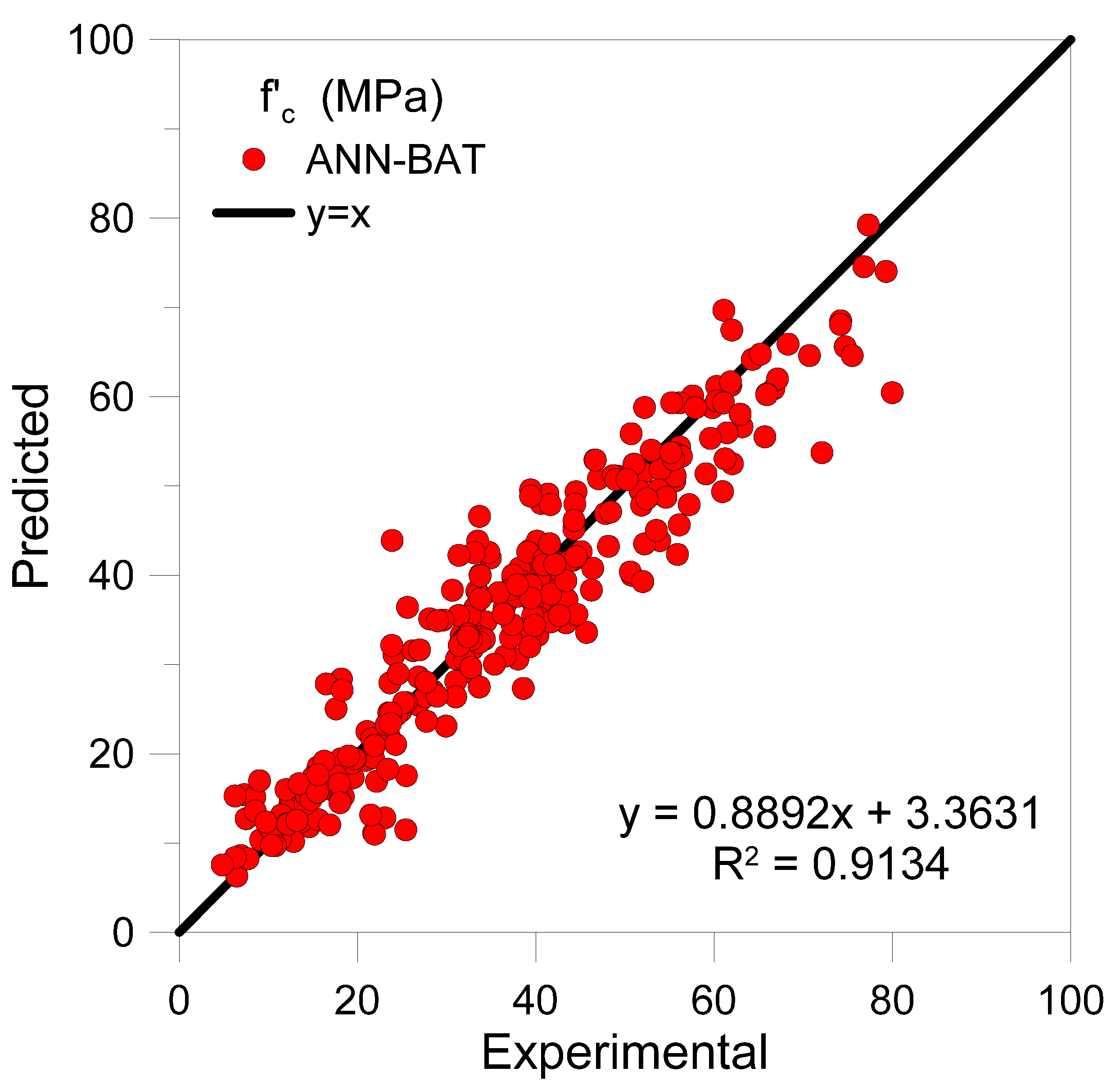
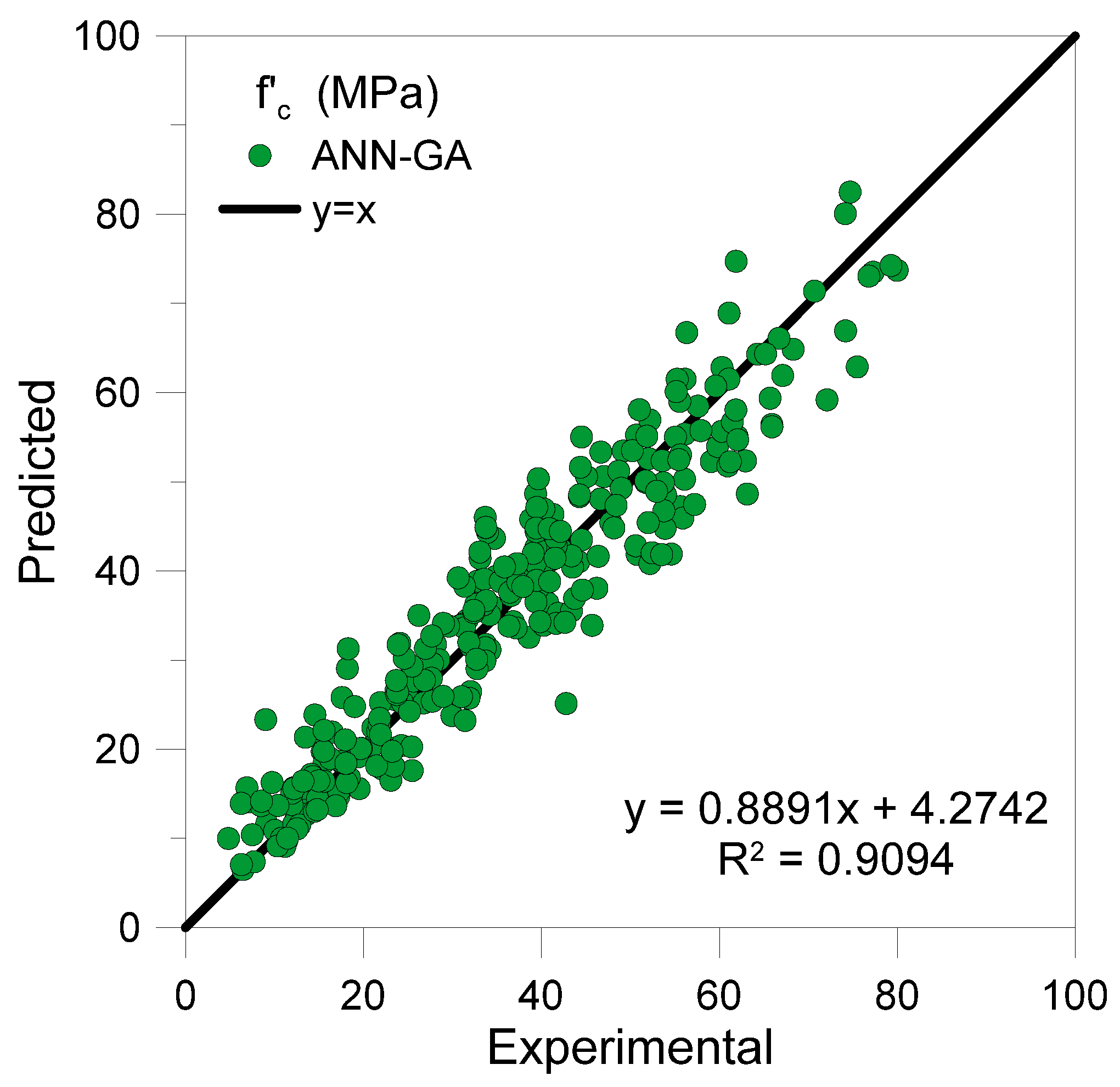
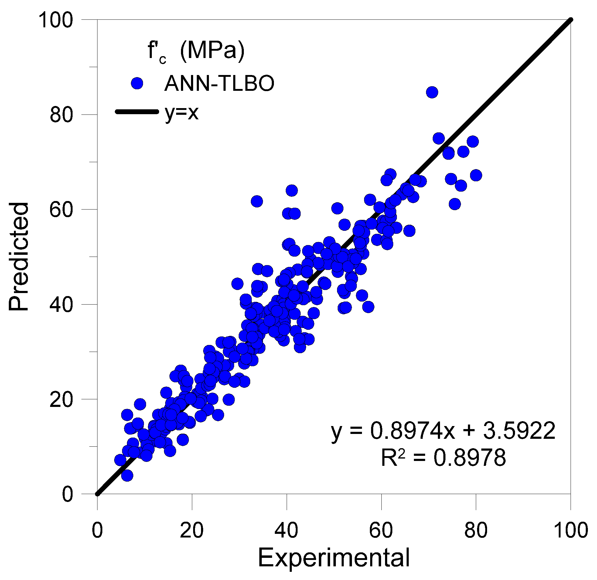
4.2. Comparison with Other Methods

To assess the accuracy of the model trained using bat optimization, three models have also been trained using other methods. Two models are ANNs trained with the genetic algorithm (GA) and Teaching-Learning-Based-Optimization (TLBO). The third is an MLR model.
The genetic algorithm is an optimization technique based on genetics and natural selection theories. It commences by generating a population of individuals and evolves them under specific selection, cross-over, and mutation rules to minimize the cost function. In this paper, individuals were the parameters of the ANN, and the final solution was the trained network.
Inspired by the teaching-learning process, the TLBO algorithm generates a population of students and designates the one with least cost to be the teacher. The remaining students then learn from the teacher, i.e., move toward the teacher’s position in solution space. In the next phase, students learn by interacting with each other, i.e., a given student (solution) interacts randomly with another student and if the second student has more knowledge (has lower cost), the first student moves towards the second [37]. In the present study, the parameters of ANN were designated as students, and the final iteration of the TLBO algorithm resulted in a trained ANN.

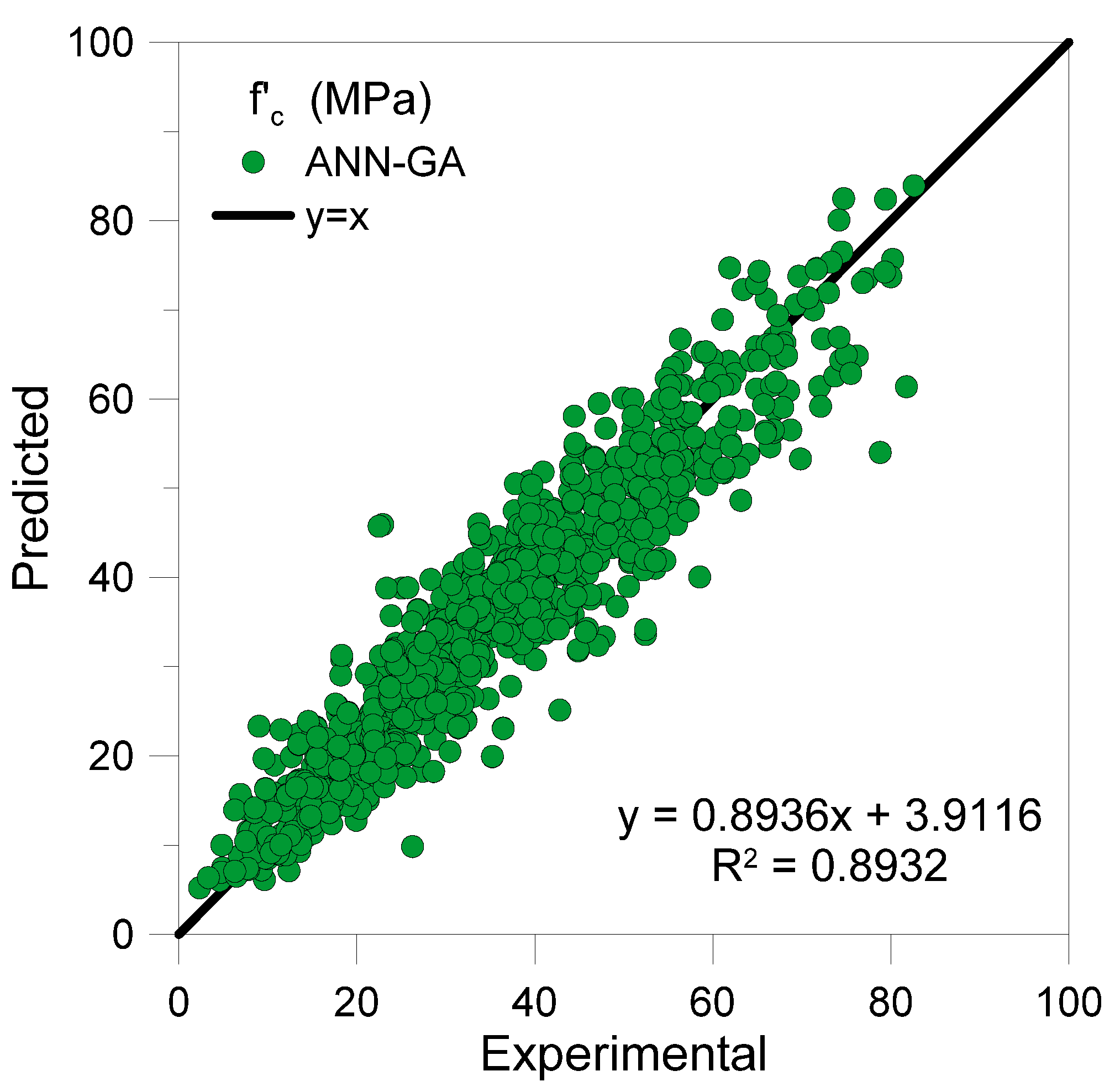
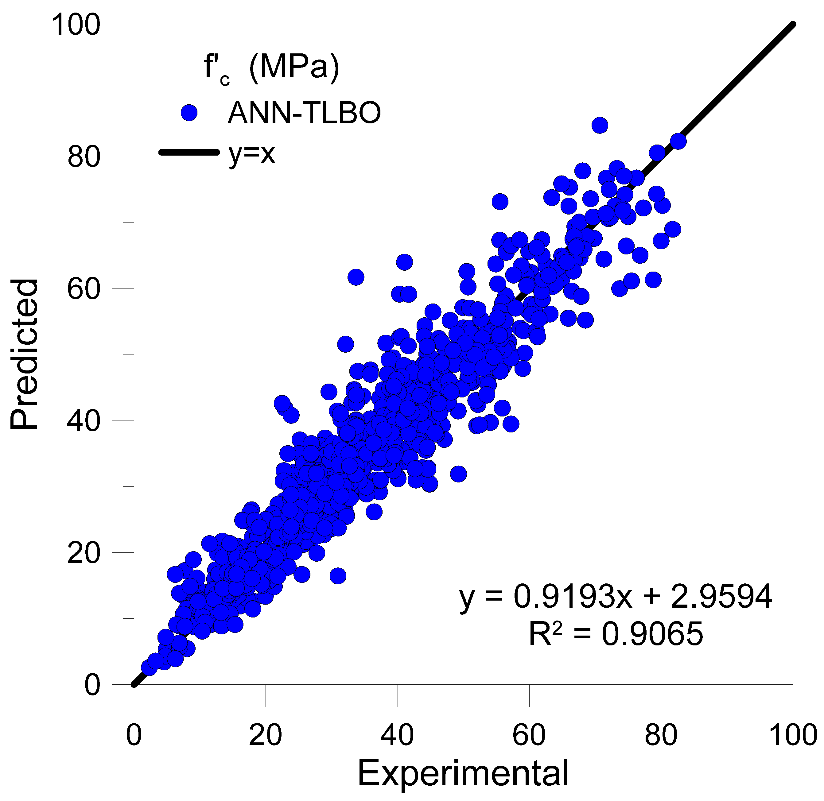
4.2.1. Genetic Algorithm and Teaching-Learning-Based-Optimization Models

The 89 topologies presented in Table 2 were used to train ANNs using the GA and TLBO to find the best ANN topology. The hyperparameters of these two algorithms are listed in Table 6.
The hyperparameters of these models were set by trial-and-error. Their values are provided in Table 7. These two networks that are optimized using GA and TLBO algorithms have a much higher prediction error compared to bat-trained neural networks. To visualize the performance of GA and TLBO, the predicted values of the experimental model versus their values from the experiments are shown in Figure 6 and Figure 7 for test data.

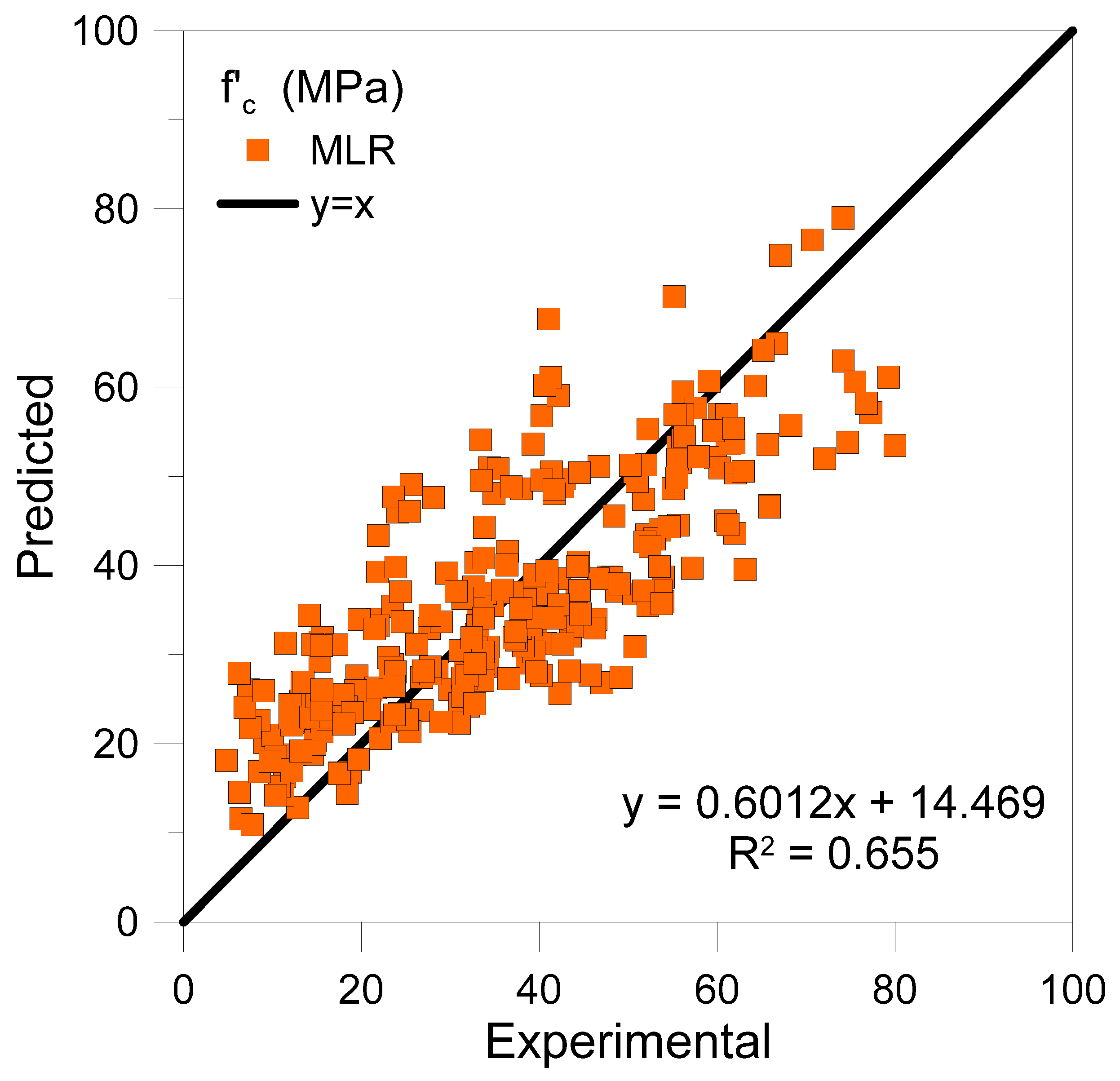
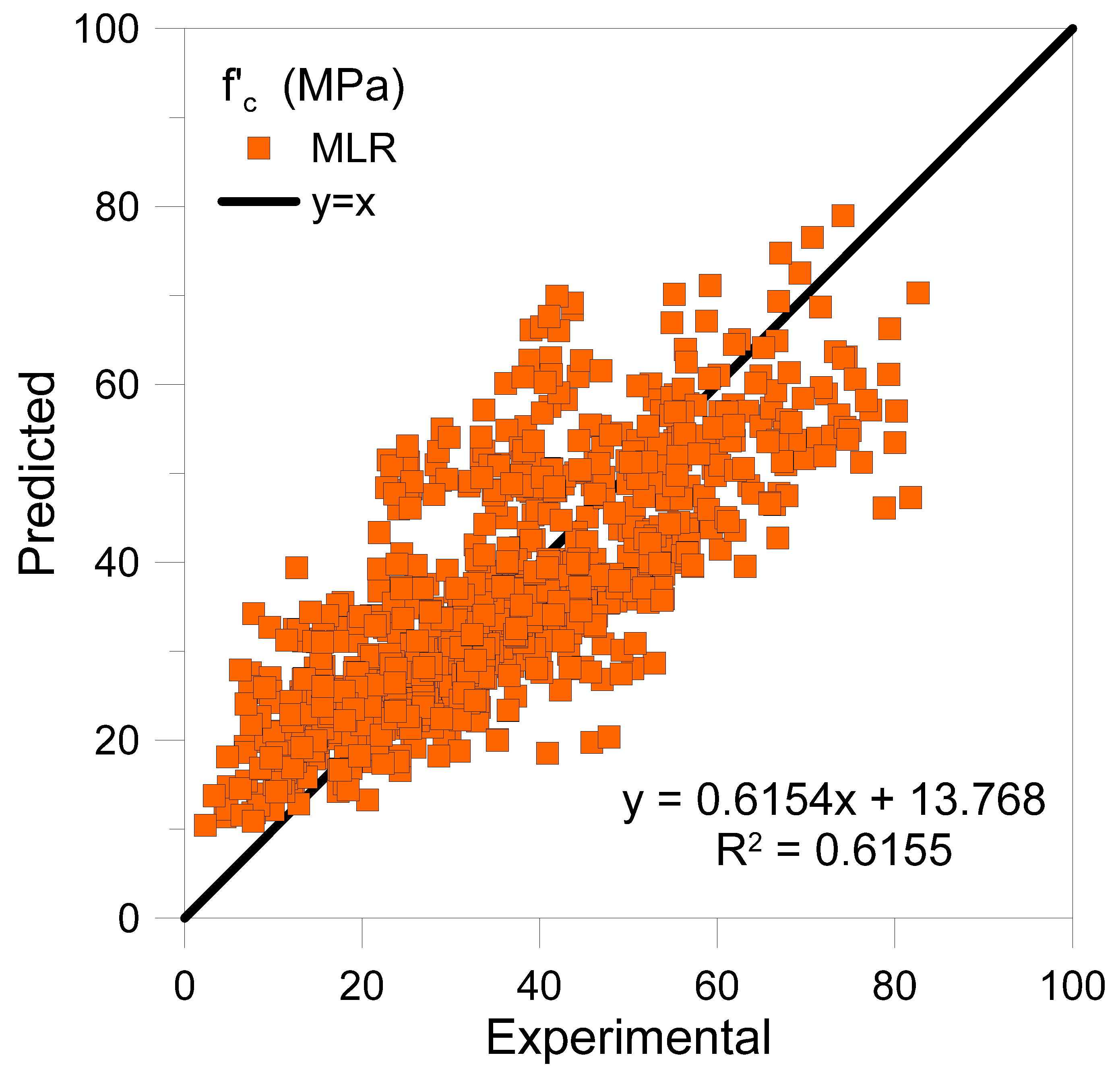
4.2.2. Multi Linear Regression Model

As suggested by Nikoo et al. [38], an MLR model was developed using the Minitab software as an easy-to-use classical model [39]. According to the model, each factor influence can be estimated by examining the regression coefficient values [40,41,42]. The resulting regression equation is as follows:
f c = 23.2 + ( 0.11979 × C ) + ( 0.1038 × BFS ) + ( 0.0879 × FA ) ( 0.1503 × W ) + ( 0.2907 × S ) + ( 0.01803 × C A ) + ( 0.0202 × F A g ) + ( 0.11423 × A )
In Equation (13), the parameters are:
C: CementW: Water
BFS: Blast Furnace SlagS: Superplasticizer
FA: Fly AshCA: Coarse Aggregate
Fag: Fine Aggregatef’c: compressive strength
A: Age
The statistical metrics of the MLR model are given in Table 8, and Figure 8 depicts the results obtained for observed versus predicted test data.

4.2.3. Comparison on All Data

The ANN-BAT-2L (7-4) is compared with the GA- and TLBO-based ANNs to validate its accuracy on all data. The MLR model is also employed as a statistical model for comparison. The results are given in Table 9.
Table 9 highlights that the ANN-TLBO model performs better than the ANN-GA model, and the MLR model has the weakest results. However, the ANN-BAT model offers the highest accuracy in determining the compressive strength of concrete of all models. The comparison between observed and predicted compressive strength of all models are shown in Figure 9, Figure 10, Figure 11 and Figure 12.

4.2.4. Comparative Analysis with Models Proposed in Literature

The developed experimental model is compared to four proposed models in literature using the same sample data. The comparison is over all data and is not divided into training and testing groups. The description of models used is given in Table 10, and the error metrics of various models are given in Table 11. As it can be seen from Table 11, the ANN-BAT-2L (7-4) model outperforms the other four models proposed in literature.

4.3. Predictive Model and ANN Weights

The best model presented in this study is ANN-BAT-2L (7-4). To calculate the output of this model manually, the matrices of network parameters are needed. The network input must be scaled using Equation (7) into −1 to 1 range, and the predicted value must then be unscaled into its original range. The input is an 8 × 1 vector called a 1 , where the eight parameters are cement, blast furnace slag, fly ash, water, superplasticizer, coarse aggregate, and fine aggregate age respectively. The following equations can be utilized to produce the ANN-BAT-2L (7-4) model predictions:
a 2 = tan h ( ϑ 1 T × a 1 + b 1 )
a 3 = tan h ( ϑ 2 T × a 2 + b 2 )
f c p r e d i c t ( n o r m a l i z e d ) = tan h ( ϑ 3 T × a 3 + b 3 )
f c p r e d i c t = f c p r e d i c t ( n o r m a l i z e d ) + 1 2 × ( f m a x f m i n ) + f m i n
where a j and ϑ j matrices represent the outputs and weights of layer j respectively and b j vector represents its biases. tanh is the hyperbolic tangent function, and T superscript represents transpose operator. fpredict is the predicted value of compressive strength, and fmax and fmin are the min and max compressive strengths of data given in Table 1. Table 12 provides the weights and biases of the neural network.

5. Conclusions

The use of accurate models plays a vital role in the design and analysis of civil engineering structural members and systems. In this regard, the present study focused on the prediction of the compressive strength of concrete based on efficient and accurate ANNs. The learning of the ANN parameters was done using the bat optimization algorithm by using 1030 experimental results published literature. Several ANN models were in fact trained (89 in total) using the bat algorithm. The top performing model was then compared with networks trained using GA and TLBO algorithms, MLR model, and four proposed compressive strength models published in literature. The main results can be summarized as follows:
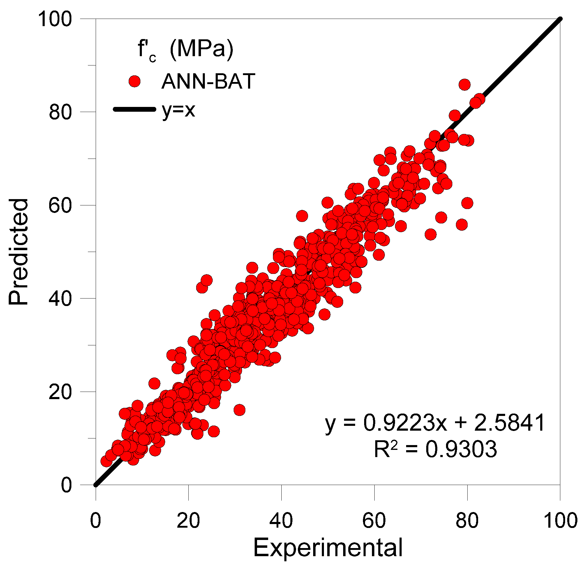
  • The top-performing bat-based ANN model, ANN-BAT-2L (7-4), yielded a mean squared error of 27.624 on testing data.
  • Due to its simplicity, a classical MLR model was presented for predicting compressive strength; however, it is less accurate than the proposed ANN-BAT model.
  • The top-performing bat algorithm-based ANN was compared with ANNs trained using GA and TLBO algorithms. The top models based on these algorithms were ANN-GA-2L (3-5) and ANN-TLBO 2L (5-6); however, they were less accurate than the ANN-BAT-2L (7-4) model. The next best performing ANN was the TLBO-based, followed by GA-based, and the MLR model.
  • The top-performing bat algorithm-based ANN was compared with four predictive models proposed in literature for compressive strength of concrete. The bat-based ANN outperformed all four.
  • The network parameters, i.e., weights and biased of the ANN-BAT-2L (7-4) model were provided in tabular format for manual calculation of network prediction. Thus, for desired and new concrete samples, the compressive strength can be estimated by providing the presented formulas with sample inputs.

Author Contributions

This research paper results from a joint collaboration of all the involved authors. All authors contributed to the paper drafting. All authors have read and agreed to the published version of the manuscript.

Funding

This research study did not receive financial funding.

Institutional Review Board Statement

Not applicable.

Informed Consent Statement

Not applicable.

Data Availability Statement

Data will be shared upon request.

Acknowledgments

MDPI is acknowledged because of the waived APCs for the corresponding author.

Conflicts of Interest

The authors declare no conflict of interest.

References

  1. Nikoo, M.; Torabian Moghadam, F.; Sadowski, Ł. Prediction of concrete compressive strength by evolutionary artificial neural networks. Adv. Mater. Sci. Eng. 2015, 2015, 1–9. [Google Scholar] [CrossRef]
  2. Asteris, P.G.; Mokos, V.G. Concrete compressive strength using artificial neural networks. Neural Comput. Appl. 2020. [Google Scholar] [CrossRef]
  3. Lai, S.; Serra, M. Concrete strength prediction by means of neural network. Constr. Build. Mater. 1997, 11, 93–98. [Google Scholar] [CrossRef]
  4. Lee, S.-C. Prediction of concrete strength using artificial neural networks. Eng. Struct. 2003, 25, 849–857. [Google Scholar] [CrossRef]
  5. Diab, A.M.; Elyamany, H.E.; Abd Elmoaty, A.E.M.; Shalan, A.H. Prediction of concrete compressive strength due to long term sulfate attack using neural network. Alex. Eng. J. 2014, 53, 627–642. [Google Scholar] [CrossRef] [Green Version]
  6. Khashman, A.; Akpinar, P. Non-Destructive Prediction of Concrete Compressive Strength Using Neural Networks. In Proceedings of the Procedia Computer Science, Zurich, Switzerland, 12–14 June 2017; Volume 108, pp. 2358–2362. [Google Scholar]
  7. Rajeshwari, R.; Mandal, S. Prediction of Compressive Strength of High-Volume Fly Ash Concrete Using Artificial Neural Network. In Sustainable Construction and Building Materials; Springer: Singapore, 2019; pp. 471–483. ISBN 978-981-13-3316-3. [Google Scholar]
  8. Kewalramani, M.A.; Gupta, R. Concrete compressive strength prediction using ultrasonic pulse velocity through artificial neural networks. Autom. Constr. 2006, 15, 374–379. [Google Scholar] [CrossRef]
  9. Słoński, M. A comparison of model selection methods for compressive strength prediction of high-performance concrete using neural networks. Comput. Struct. 2010, 88, 1248–1253. [Google Scholar] [CrossRef]
  10. Atici, U. Prediction of the strength of mineral admixture concrete using multivariable regression analysis and an artificial neural network. Expert Syst. Appl. 2011, 38, 9609–9618. [Google Scholar] [CrossRef]
  11. Yeh, I.C. Modeling Concrete Strength with Augment-Neuron Networks. J. Mater. Civ. Eng. 1998, 10, 263–268. [Google Scholar] [CrossRef]
  12. Yeh, I.C. Modeling of strength of high-performance concrete using artificial neural networks. Cem. Concr. Res. 1998, 28, 1797–1808. [Google Scholar] [CrossRef]
  13. Öztaş, A.; Pala, M.; Özbay, E.; Kanca, E.; Çagˇlar, N.; Bhatti, M.A. Predicting the compressive strength and slump of high strength concrete using neural network. Constr. Build. Mater. 2006, 20, 769–775. [Google Scholar] [CrossRef]
  14. Faridmehr, I.; Bedon, C.; Huseien, G.F.; Nikoo, M.; Baghban, M.H. Assessment of Mechanical Properties and Structural Morphology of Alkali-Activated Mortars with Industrial Waste Materials. Sustainability 2021, 13, 2062. [Google Scholar] [CrossRef]
  15. Behnood, A.; Golafshani, E.M. Predicting the compressive strength of silica fume concrete using hybrid artificial neural network with multi-objective grey wolves. J. Clean. Prod. 2018, 10, 1859–1867. [Google Scholar] [CrossRef]
  16. Nazari, A.; Riahi, S. Prediction split tensile strength and water permeability of high strength concrete containing TiO2 nanoparticles by artificial neural network and genetic programming. Compos. Part B Eng. 2011, 42, 473–488. [Google Scholar] [CrossRef]
  17. Bui, D.K.; Nguyen, T.; Chou, J.S.; Nguyen-Xuan, H.; Ngo, T.D. A modified firefly algorithm-artificial neural network expert system for predicting compressive and tensile strength of high-performance concrete. Constr. Build. Mater. 2018, 180, 320–333. [Google Scholar] [CrossRef]
  18. Sadowski, L.; Nikoo, M.; Nikoo, M. Concrete compressive strength prediction using the imperialist competitive algorithm. Comput. Concr. 2018, 22, 355–363. [Google Scholar] [CrossRef]
  19. Duan, J.; Asteris, P.G.; Nguyen, H.; Bui, X.-N.; Moayedi, H. A novel artificial intelligence technique to predict compressive strength of recycled aggregate concrete using ICA-XGBoost model. Eng. Comput. 2020, 1–18. [Google Scholar] [CrossRef]
  20. Zhou, Q.; Wang, F.; Zhu, F. Estimation of compressive strength of hollow concrete masonry prisms using artificial neural networks and adaptive neuro-fuzzy inference systems. Constr. Build. Mater. 2016, 125, 417–426. [Google Scholar] [CrossRef]
  21. Armaghani, D.J.; Asteris, P.G. A comparative study of ANN and ANFIS models for the prediction of cement-based mortar materials compressive strength. Neural Comput. Appl. 2021, 33, 4501–4532. [Google Scholar] [CrossRef]
  22. Hoła, J.; Schabowicz, K. Application of artificial neural networks to determine concrete compressive strength based on non-destructive tests. J. Civ. Eng. Manag. 2005, 11, 23–32. [Google Scholar] [CrossRef]
  23. Khademi, F.; Akbari, M.; Jamal, S.M.; Nikoo, M. Multiple linear regression, artificial neural network, and fuzzy logic prediction of 28 days compressive strength of concrete. Front. Struct. Civ. Eng. 2017, 11, 90–99. [Google Scholar] [CrossRef]
  24. Fan, M.; Zhang, Z.; Wang, C. Chapter 7—Optimization Method for Load Frequency Feed Forward Control; Academic Press: New York, NY, USA, 2019; pp. 221–282. ISBN 978-0-12-813231-9. [Google Scholar]
  25. Fan, M.; Zhang, Z.; Wang, C. Optimization Method for Load Frequency Feed Forward Control. In Mathematical Models and Algorithms for Power System Optimization; Elsevier: Amsterdam, The Netherlands, 2019. [Google Scholar]
  26. Ellis, G. Feed-Forward. In Control System Design Guide; Ellis, G., Ed.; Academic Press: Burlington, NJ, USA, 2004; pp. 151–169. ISBN 978-0-12-237461-6. [Google Scholar]
  27. Jun, L.; Liheng, L.; Xianyi, W. A double-subpopulation variant of the bat algorithm. Appl. Math. Comput. 2015, 263, 361–377. [Google Scholar] [CrossRef]
  28. Yang, X.S. Nature-Inspired Optimization Algorithms; Elsevier: Amsterdam, The Netherlands, 2014; ISBN 9780124167438. [Google Scholar]
  29. Dehghani, H.; Bogdanovic, D. Copper price estimation using bat algorithm. Resour. Policy 2018, 55, 55–61. [Google Scholar] [CrossRef]
  30. Haykin, S. Neural Networks and Learning Machines; Pearson: London, UK, 2008; Volume 3, ISBN 9780131471399. [Google Scholar]
  31. Hasanzade-Inallu, A.; Zarfam, P.; Nikoo, M. Modified imperialist competitive algorithm-based neural network to determine shear strength of concrete beams reinforced with FRP. J. Cent. South Univ. 2019, 26, 3156–3174. [Google Scholar] [CrossRef]
  32. Li, J.; Heap, A.D. A Review of Spatial Interpolation Methods for Environmental Scientists; Australian Government: Canberra, Australia, 2008; ISBN 9781921498305. [Google Scholar]
  33. Géron, A. Hands-on Machine Learning with Scikit-Learn and TensorFlow: Concepts, Tools, and Techniques to Build Intelligent Systems; O’Reilly Media, Inc.: Sebastopol, CA, USA, 2017. [Google Scholar]
  34. Plevris, V.; Asteris, P.G. Modeling of masonry failure surface under biaxial compressive stress using Neural Networks. Constr. Build. Mater. 2014, 55, 447–461. [Google Scholar] [CrossRef]
  35. Bowden, G.J.; Dandy, G.C.; Maier, H.R. Input determination for neural network models in water resources applications. Part 1—background and methodology. J. Hydrol. 2005, 301, 75–92. [Google Scholar] [CrossRef]
  36. MATLAB; The MathWorks: Natick, MA, USA, 2018.
  37. Rao, R.V.; Savsani, V.J.; Vakharia, D.P. Teaching-learning-based optimization: A novel method for constrained mechanical design optimization problems. CAD Comput. Aided Des. 2011, 43, 303–315. [Google Scholar] [CrossRef]
  38. Nikoo, M.; Sadowski, L.; Khademi, F.; Nikoo, M. Determination of Damage in Reinforced Concrete Frames with Shear Walls Using Self-Organizing Feature Map. Appl. Comput. Intell. Soft Comput. 2017, 2017, 1–10. [Google Scholar] [CrossRef]
  39. Delozier, M.R.; Orlich, S. Discovering influential cases in linear regression with MINITAB: Peeking into multidimensions with a MINITAB macro. Stat. Methodol. 2005, 2, 71–81. [Google Scholar] [CrossRef]
  40. Panesar, D.K.; Aqel, M.; Rhead, D.; Schell, H. Effect of cement type and limestone particle size on the durability of steam cured self-consolidating concrete. Cem. Concr. Compos. 2017, 80, 157–159. [Google Scholar] [CrossRef]
  41. Gevrey, M.; Dimopoulos, I.; Lek, S. Review and comparison of methods to study the contribution of variables in artificial neural network models. Ecol. Model. 2003, 160, 249–264. [Google Scholar] [CrossRef]
  42. Hasanzade-Inallu, A. Grey Wolf Optimizer-Based ANN to Predict Compressive Strength of AFRP-Confined Concrete Cylinders. Soil Struct. Interact. 2018, 3, 23–32. [Google Scholar]
  43. Gandomi, A.H.; Alavi, A.H.; Shadmehri, D.M.; Sahab, M.G. An empirical model for shear capacity of RC deep beams using genetic-simulated annealing. Arch. Civ. Mech. Eng. 2013, 13, 354–369. [Google Scholar] [CrossRef]
  44. Chou, J.-S.; Pham, A.-D. Enhanced artificial intelligence for ensemble approach to predicting high performance concrete compressive strength. Constr. Build. Mater. 2013, 49, 554–563. [Google Scholar] [CrossRef]
  45. Chou, J.S.; Chong, W.K.; Bui, D.K. Nature-Inspired Metaheuristic Regression System: Programming and Implementation for Civil Engineering Applications. J. Comput. Civ. Eng. 2016, 30, 4016007. [Google Scholar] [CrossRef]
Figure 1. Architecture of the optimum ANN developed in the present study. This architecture includes eight input nodes, seven nodes in the first hidden layer, four nodes in the second hidden layer, and one node (f’c) in the output layer.
Infrastructures 06 00080 g001
Figure 2. Outline of the research study.
Infrastructures 06 00080 g002
Figure 3. Distribution of concrete compressive strength fc for the selected experimental data.
Infrastructures 06 00080 g003
Figure 4. Predicted versus experimental compressive strength f’c for ANN-BAT-2L (7-4) model using training data.
Infrastructures 06 00080 g004
Figure 5. Predicted versus experimental compressive strength f’c for ANN-BAT-2L (7-4) model using testing data.
Infrastructures 06 00080 g005
Figure 6. Predicted versus experimental compressive strength f’c for ANN-GA (3-5) model using testing data.
Infrastructures 06 00080 g006
Figure 7. Predicted versus experimental compressive strength f’c for ANN-TLBO (5-6) model using testing data.
Infrastructures 06 00080 g007
Figure 8. Predicted versus experimental compressive strength f’c for MLR model using testing data.
Infrastructures 06 00080 g008
Figure 9. Predicted versus experimental compressive strength f’c, based for the ANN-GA model using all data.
Infrastructures 06 00080 g009
Figure 10. Predicted versus experimental compressive strength f’c, based for the ANN-BAT model using all data.
Infrastructures 06 00080 g010
Figure 11. Predicted versus experimental compressive strength f’c, based for the ANN-TLBO model using all data.
Infrastructures 06 00080 g011
Figure 12. Predicted versus experimental compressive strength f’c, based for the MLR model using all data.
Infrastructures 06 00080 g012
Table 1. Descriptive statistics of samples.
Statistical IndexUnitMinMinAverageStandard DeviationModeMedian
CementKg/m3540102281.17104.51425272.9
Blast Furnace SlagKg/m3359.4073.9086.28022
Fly AshKg/m3200.1054.1964.0000
WaterKg/m3247121.75181.5721.36192185
SuperplasticizerKg/m332.206.205.9706.35
Coarse AggregateKg/m31145801972.9277.75932968
Fine AggregateKg/m3992.6594773.5880.18594779.51
Ageday365145.6663.172828
Concrete compressive strengthMPa82.602.3335.8216.7133.4034.44
Table 2. Trained ANN topologies.
NumTopologyNumTopology...NumTopologyNumTopology
11-192-1...659-1731
21-2102-2...669-2742
31-3112-3...679-3753
41-4122-4...689-4764
...........................
71-7152-7...719-78816
81-8162-8...729-88917
Note: n1-n2 format for topologies denotes n1 neurons in the first hidden layer, and n2 neurons in the second hidden layer.
Table 3. Hyperparameters of the bat algorithm.
HyperparameterValueHyperparameterValue
Population Total100Max Generations200
Loudness0.9Pulse Rate0.5
Min Freq.0Max Freq.2
Alpha0.99Gamma0.01
Table 4. Error metrics of top four networks on training data.
NumNetwork
Designation
Training
MSEMEMAERMSE
1ANN-BAT-1L (4)28.4710.0003.9895.336
2ANN-BAT-2L (3-2)28.5430.0004.0185.343
3ANN-BAT-2L (8-5)10.9280.0002.4483.306
4ANN-BAT-2L (7-4)16.0010.0002.8954.000
Note: ANN-BAT-(m)L (n1-n2) format denotes m hidden layers, n1 neurons in the first hidden layer and n2 neurons in second hidden layer.
Table 5. Error metrics of top four networks on testing data.
NumNetwork
Designation
Testing
MSEMEMAERMSE
1ANN-BAT-1L (4)37.146−0.1474.6746.095
2ANN-BAT-2L (3-2)37.4960.1484.7396.123
3ANN-BAT-2L (8-5)40.130−0.5463.8286.335
4ANN-BAT-2L (7-4)27.624−0.6643.8475.256
Note: ANN-BAT-(m)L (n1-n2) format denotes m hidden layers, n1 neurons in the first hidden layer and n2 neurons in second hidden layer.
Table 6. GA and TLBO hyperparameters.
NameParameterValueParameterValue
Genetic AlgorithmMax generations100Crossover (%)50
Recombination (%)15Crossover methodsingle point
Lower Bound−1Selection Mode1
Upper Bound+1Population Size150
Teaching Learning Base OptimizationLower Bound−1Max Interaction50
Upper Bound+1Population Size150
The TLBO algorithm-trained ANN with 5-6 topologies and the GA-trained ANN with the 3-5 topologies have the highest performance, as shown by the statistical indices in Table 7.
Table 7. Error metrics of GA and TLBO on training and testing data.
TopologyTrainTest
MEMAEMSERMSEMEMAEMSERMSE
ANN-GA-2L (3-5)0.044.1330.355.510.254.1728.445.33
ANN-TLBO-2L (5-6)0.163.5923.684.87−0.144.0231.875.65
Note: ANN-(A)-(m)L (n1-n2) format denotes algorithm A, m hidden layers, n1 neurons in the first hidden layer and n2 neurons in second hidden layer.
Table 8. MLR model error metrics for training and testing data.
TopologyTrainingTesting
MEMAEMSERMSEMEMAEMSERMSE
MLR0.008.08106.4910.32−0.028.52108.9110.44
Table 9. Statistics of ANN-BAT, ANN-GA, ANN-TLBO and MLR models.
TypeNetwork DesignationMEMAEMSERMSE
All DataANN-BAT-2L(7-4)−0.1993.18119.4884.414
ANN-GA-2L(3-5)0.104.1429.775.46
ANN-TLBO-2L(5-6)0.073.7226.135.11
MLR−0.018.22107.2110.35
Table 10. Description of models proposed in literature.
AuthorModelReference
A.H. Gandomi et al.Genetic-Simulated Annealing[43]
J.-S. Chou et al.Support Vector Machines[44]
Jui-Sheng et al.Least Squares Support Vector Machines[45]
D.-K. Bui et al.Firefly Algorithm combined Artificial Neural Network[17]
Table 11. Error metrics of models proposed in literature, and bat-based ANN (ordered by R2).
ModelR2MAE
Present (ANN-BAT-2L (7-4))0.933.18
D.-K. Bui et al. (2018)0.903.41
J.-S. Chou et al. (2013)0.884.24
Jui-Sheng et al. (2016)0.885.62
A.H. Gandomi et al. (2013)0.815.48
Table 12. Weight and bias values of the ANN-BAT-2L (7-4) model.
ϑ 1 b 1
−0.8061−0.2178−0.2297−0.4198−0.5889−0.3034−0.2999−0.1035−0.8156
0.2371−0.6965−0.11321.34101.51700.37820.02380.18070.6200
−6.3017−2.6506−2.49312.52632.0438−0.8616−4.4602−1.1676−1.1071
0.0226−0.0670−0.11910.05050.03420.0304−0.07813.62084.6903
−6.9203−18.4075−3.0575−27.3813−10.0966−11.8482−7.9640−1.1299−16.3967
31.2215−7.9121−19.6231−0.055114.0536−15.0847−12.6117−2.1349−4.3244
0.6362−3.26114.4076−5.99584.4666−4.3309−1.5010−8.07831.1720
ϑ 2 b 2
−1.6512−0.74340.30500.13810.1699−0.1258−0.1164 −2.0524
6.62962.6327−1.730713.1062−0.6463−0.05061.1651−9.5413
33.042823.34623.0604−21.0571−1.85400.2323−19.2491−12.8245
1.01290.6331−0.66319.3516−0.73770.47730.3696−8.0055
ϑ 3 b 3
12.86580.46400.24890.4572 11.7091
Publisher’s Note: MDPI stays neutral with regard to jurisdictional claims in published maps and institutional affiliations.

