Deep Reinforcement Learning Model to Mitigate Congestion in Real-Time Traffic Light Networks

Abstract

Urban traffic congestion has a significant detrimental impact on the environment, public health and the economy, with at a high cost to society worldwide. Moreover, it is not possible to continually modify urban road infrastructure in order to mitigate increasing traffic demand. Therefore, it is important to develop traffic control models that can handle high-volume traffic data and synchronize traffic lights in an urban network in real time, without interfering with other initiatives. Within this context, this study proposes a model, based on deep reinforcement learning, for synchronizing the traffic signals of an urban traffic network composed of two intersections. The calibration of this model, including training of its neural network, was performed using real traffic data collected at the approach to each intersection. The results achieved through simulations were very promising, yielding significant improvements in indicators measured in relation to the pre-existing conditions in the network. The model was able to deal with a broad spectrum of traffic flows and, in peak demand periods, reduced delays and queue lengths by more than 28% and 42%, respectively.

1. Introduction

Vehicular congestion is a growing global problem in urban areas and is one of the major challenges that must be addressed by transportation systems to mitigate deteriorating traffic conditions. Environmentally, traffic congestion increases noise and air pollution. With respect to public health, it is linked to excessive fatigue and mental illness, as well as to cardiovascular, respiratory, and nervous system problems. In economic terms, congestion increases transport times, fuel consumption and operating costs, adversely affecting the distribution and sale of goods, leading to consumer price increases [1,2,3,4].

In Brazil, traffic congestion occurs daily in major metropolitan regions, impacting traffic distribution, trip frequency, driver behavior, safety, land use, and more broadly, the economy, leading to significant losses for society [5]. In 2012, the cost attributable solely to traffic jams in the city of São Paulo totaled USD 20.5 billion [6]. Moreover, the traffic congestion has reduced the productivity in the United States and worldwide [7,8].

Therefore, because urban infrastructure improvement projects take time and are often not feasible, it is important to develop strategic technologies to improve the efficiency of existing infrastructure, minimizing congestion and its consequences as much as possible [2,9,10]. A traffic control model with these attributes is a technology that meets these objectives.

In general, the previous literature addresses traffic congestion under the economic bias, proposing strategies to price congestion and charge the road network. The decisions of the drivers are then related to this charging policy taking into account the travel mode, the departure time, and the chosen route. These previous works deal with congestion pricing strategies based on rationally constrained user equilibrium bound route choices employing a heuristic algorithm to find the congestion price to minimize the network travel time. Thus, the drivers do not necessarily choose a shorter or cheaper route if travel time is not significantly reduced [11].

Other previous studies have also applied congestion pricing strategies implementing optimization models to consider the drivers income on their decisions to the trip generation, the transport modes, and the chosen routes in the networks. The models aim to design more efficient traffic jam pricing and tradable credit schemes to reduce traffic congestion among different income and geographic groups [4]. It is suggested that these road network charging strategies can be effective tools to manage the traffic flow demand based on market rules, influencing once more the drivers’ decisions. The concept of multi-period tradable credit schemes has also been used affecting the drivers’ choices. The developed idea regards the consumption or sale of credits in current or future periods of time, increasing or alleviating the flow of traffic in the network. Finally, this tradable strategy would be useful to mitigate credit price volatility allowing the central transit authority to develop credit prices schemes where the users protect themselves of potential monetary losses [12].

The synchronization of traffic lights to reduce traffic congestion has also been applied since the 1980s [13]. The researchers when synchronizing the traffic lights have sought to develop the associated traffic lights theory adapting urban traffic control to real-world needs. Urban traffic control models that have then emerged have been widely implemented in different places including in Europe, the United States, and Brazil. Among the most applied models are DYPIC, SCOOTS, SCATS, ITACA, OPAC, PRO-DYN, UTOPIA, ALLONS-D, RHODES, ACS, and TUC, but it must be said that all of them depend on a traffic model, and most of them are based in dynamic programming [14,15,16,17,18,19,20].

The costs of implementing these adaptive control models can vary from USD 6000 to USD 60,000 per intersection, which, despite their importance, these high costs can restrict their use in many cities. Additionally, their operation can result in significant variations in the number of stops, vehicle delays, and travel times. In particular, the SCOOTS model can reduce from 17% to 32% the number of stops. Moreover, the SCATS model can reduce up to 19% or increase by 3% the vehicle delays, while OPAC can reduce or increase travel time by 26% or 10%, respectively [19]. Once analyzing the described results by the SCOOTS, SCATS, and OPAC models, many researchers working on the development of these technologies have proposed several optimization models for traffic lights planning. These proposed optimization models include fuzzy logic, genetic algorithms, dynamic programming, and neural networks and, lately, the new models have also dealt with Artificial Intelligence (AI) and Deep Reinforcement learning techniques (Deep Q-learning). These new policies and tools have lately been discussed when talking about the smart cities systems.

The smart city concept is becoming the future trend of the urban development where it includes the topics of smart homes, smart transport, green city, smart roads, smart urban management, and smart tourism among others. Smart city is related to the Internet of Things (IoT), the Internet of Everything (IoE), and Information Communication Technology (ICT) collecting and evaluating a lot of data in real time. Smart cities can then revolutionize the management of metropolitan transport and infrastructure operations, mitigating existing traffic problems [4,21,22].

The development of smart cities can really increase the efficiency of the transport infrastructure and its operation dealing with current traffic conditions through intelligent and efficient traffic management tools [4]. Particularly, the Intelligent Traffic Management System (TMS) is one of these important tools to be applied to reduce traffic congestion and to better control the traffic signals (TSC) [3,22]. After all, despite the drivers’ behavior changing because of any applied TMS, traffic management must be skilled to respond to the new scenarios due to these drivers’ changes.

The Intelligent Traffic Management System uses the digital devices available in the smart road environment (SRE) and in autonomous vehicles. The TMS will collect the vehicles data, transmitting them to the traffic monitoring system where, after analyzing the driver behavior, it can better synchronize the traffic lights network in real time [22].

In this context, this paper proposes a new urban traffic control model based on the application of deep reinforcement learning developed from the algorithm proposed by [23]. The algorithm used as a reference performs the optimization of the signal timing for only one intersection based on traffic flow of between 100 and 2000 vehicles/hour randomly generated according to a Poisson distribution. The researchers adopted queue length as the traffic state variable, minimizing queue length as the reward variable for traffic light action.

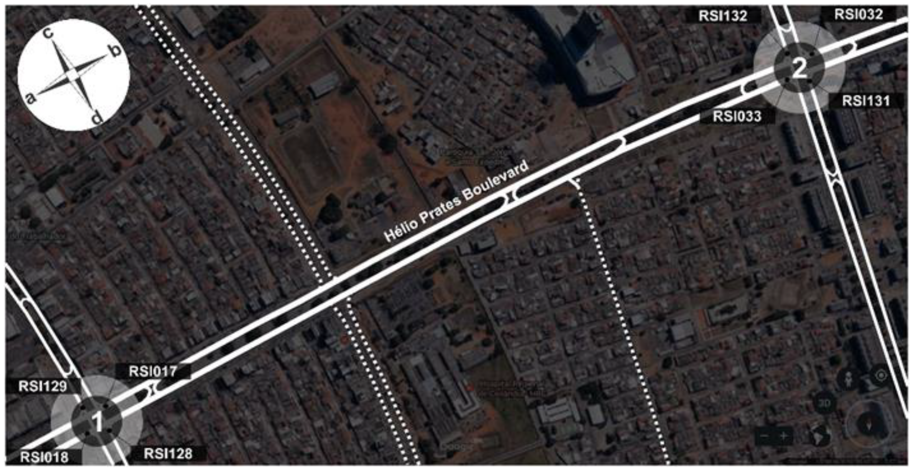
The problem addressed by our study is approached by means of a traffic network located between two Administrative Regions of the Federal District, composed of two intersections. Each intersection is located in a different administrative region and connects one of the two collector roads to an arterial road—Hélio Prates Boulevard. Traffic jams occur on this road, daily, especially in the morning when users are commuting to work. Each collector road is a dual carriageway with two lanes in opposing directions. The arterial road is also a dual carriageway, but it has three traffic lanes in each direction. Accordingly, the selected traffic network has two intersections connecting ten traffic lanes with eight sensor data collection sections.

A solution to the problem must ensure that the arterial road, which connects the two intersections, delivers the greatest possible traffic flow throughput without hindering the performance of the collector roads at each intersection. Thus, the main objective of this research is to maximize the number of vehicles crossing the intersections, optimizing the signal timing between them using the Deep Reinforcement Learning technique. This technique has a flexible structure that can be modified to adapt to changes in the traffic network.

In this context, this paper proposes an approach based on deep reinforcement learning to synchronize the traffic signal plans of two networked intersections from flow data collected by inductive loop detectors to improve the performance of the traffic network as a whole. These sensors are extremely common in existing traffic controls around the world [24] and also in Brazilian cities, especially in the metropolitan regions of most medium and large cities in the country.

The main contribution of this work is the development and implementation of a model capable of controlling urban traffic according to the decisions effectively taken by the drivers. These decisions are taken in real time and in a centralized way, instead of controlling isolated intersections, through the development of a reward that integrates the network intersections. Furthermore, the proposed approach does not depend on a traffic model, and it is not limited to just one type of data collection device. The presented approach is then able to operate adequately and timely just with the collected count of vehicles per unit of time that is the traffic flow.

The paper is divided into five sections. The Section 1 presents the problem and objectives of the paper. The Section 2 presents a review of the state of the art for the main themes addressed in the study. The Section 3 describes the research methodology and the various stages of the proposed model. The Section 4 analyzes the results obtained, and finally, the Section 5 presents the conclusions.

2. The State of the Art

This study relies on the collection of an enormous amount of data and a tool capable of handling this volume of data to produce information and make consistent and timely decisions for real-time urban traffic control. Therefore, it is important to address the technology of inductive loop detectors with its technical characteristics and the relevance of its wide application around the world. In the same context, it is important to highlight the importance of the artificial intelligence techniques studied in order to propose better solutions to the complex problems that determine the synchronization of traffic signal timing plans. Therefore, the next two items in this section will address the use of data provided by inductive loop detectors and traffic control with synchronization of signal timing through the use of artificial intelligence tools

2.1. Using Data Provided by Inductive Loop Detectors

Any traffic response control system depends on its ability to detect traffic to control local intersections by synchronizing traffic signal timing plans throughout the system [25]. Analysis and understanding of transportation-related issues are therefore often restricted to a domain that depends on a data source.

Various algorithms have been developed based on different methods of traffic density detection, including infrared sensors, GPS systems, video cameras, and others. There are many technologies available to detect traffic, but inductive loop detectors remain arguably the best method, and the simplest as well, to collect vehicular flow data [26]. Therefore, data collected by inductive loops are widely used to synchronize traffic signal timing plans in the urban environment [23,24].

Inductive loop detectors are an alternative to data survey technologies and have traditionally been used to collect basic traffic data, including volume and speed. These detectors are used as a simple and consistent source of data because they accurately reflect the actual traffic network environment at any specific time. Furthermore, aggregating the data from inductive loop detectors at any time interval is simple, making time-dependent measurements extremely flexible [1,27].

The configuration of inductive loop detectors consists of one or more insulated wire loops wound in a shallow slot sawed into the sidewalk (Figure 1). Basically, it operates by means of an electric current induced in the loop by the passage of the vehicle. This detector can take on various configurations of size and shape depending on the area of interest, the types of vehicles to be detected, and the purpose of data collection, such as queue detection, vehicle counting, or speed measurements [1,25]. Figure 1 depicts the arrangement of inductive loop detectors installed over the crosswalk located at one of the intersections in the area studied.

2.2. Traffic Control with Synchronized Traffic Timing Using Artificial Intelligence Tools

Urban traffic control systems, as an essential part of dynamic traffic management, aim to reduce congestion, mitigate environmental impacts, and at the same time increase traffic safety and the efficiency of the road network. State-of-the-art urban traffic control systems use traffic models to estimate, predict, and optimize traffic flow based on real-time measurements [2,3,24].

Synchronizing traffic signal timing is one of the fastest and most cost-effective ways to reduce intersection congestion and optimize traffic flow on urban roads. This requires a plan that can adapt to demand fluctuations, with many parameters of signal timing affecting intersection performance [2]. In this regard, several studies have been conducted to improve the intelligence of traffic control systems for intersections. However, complicated traffic light optimization problems cannot be solved using conventional methods, and therefore, traffic light synchronization has recently employed artificial intelligence (AI) techniques including fuzzy logic, reinforcement learning (Q-learning), and deep reinforcement learning (Deep Q-learning) [3].

Fuzzy logic has been used to optimize traffic signal timing. Compared to fixed-time controllers, it is an adaptive method where the dynamic environment is analyzed, and predefined models are adapted to the demands of that environment continuously. However, the system requires a lot of processing power to perform all the necessary tasks, and eventually, this degrades its performance to some extent.

Consequently, researchers started experimenting with other techniques such as reinforcement learning and then deep reinforcement learning based on Q-learning and Deep Q-learning algorithms, respectively, to perform traffic flow management. Unlike fuzzy logic, Q-learning does not use predefined models, thus making it more suitable for real-time traffic management problems [3]. The reinforcement learning approach implicitly models the dynamics of complex systems, learning the control actions and resulting changes in traffic flow. Meanwhile, it searches for the optimal traffic signal plan for the learned input and output pairs [23].

Some studies have used Q-learning to achieve optimization of traffic signal timing and, consequently, congestion reduction by minimizing traffic control parameters such as stop delay, queue length, and waiting time per vehicle. Although they adapt to real-time demand, these models cannot change the signal sequence between different traffic lights. A later Q-learning model, combining the clustering technique with the waiting time queue length parameters, was able to vary the order of traffic lights according to traffic flow [3].

Recently, a study conducted by [3] sought an adaptive solution for a complex dynamic traffic system, proposing a solution for traffic signal control in light of the emergence of smart cities and the development of the Internet of Things by employing a Q-learning algorithm and maximizing the number of vehicles. Despite the proposal of a flexible structure, easily applicable in several N-way intersections according to the authors, this proposal was applied in only one intersection.

However, it is necessary to consider the size of the traffic network, and reinforcement learning has a major difficulty in optimizing traffic signal timing, in that the complexity of a traffic signal plan grows exponentially with the number of traffic flow states and control actions considered [23].

Therefore, a new method was proposed to simultaneously solve the modeling and optimization problems of complex systems by combining two important tools: reinforcement learning and deep learning. This resulted in Deep Q-learning, which better adheres to the problem conditions in that deep learning complements reinforcement learning by using multiple layers of artificial neural networks to learn the implied maximum discounted future reward when a certain action in a given state is executed [23,28,29].

Deep Q-learning learns the Q-function by means of a deep neural network (DNN). Then, the value-function-based agent selects the optimal control action, making it capable of handling high-dimensional inputs for multiple states beyond Q-learning [3]. Then, it simultaneously learns the dynamics of the traffic system and the optimal control plan, implicitly modeling the control actions and the change of system states. As a result, it outperforms conventional approaches in optimizing traffic signal timing [23,29].

Some studies have demonstrated the feasibility and effectiveness of deep reinforcement learning in traffic signal synchronization plans. Numerical tests show that deep networks are the most convenient and powerful means to approximate the maximum discounted future reward [23]. Again, combinations between traffic control parameters such as queue lengths and total cumulative delays at an intersection were used as reward variables [3,23,28].

There is an extensive literature review that develops the deep reinforcement learning approaches applied to traffic signal control, describing their architectures and respective attributes: methods, rewards, actions, and states, in line with the main models that have already been implemented [29]. This study is considered to be of extreme importance for the reader interested in deepening their knowledge on this topic.

3. Research Methodology

The research methodology for this study aimed to develop an intelligent model for traffic signal synchronization that adapts to the actual demand conditions triggered by the traffic flow present at the approaches to the intersections of a road network. Once the data set was collected, it was applied to calibrate the model and validated it. Afterwards, applying the Vissim microsimulation software, the obtained results for the measured parameters when applying not only the actual traffic plan but also the intelligent one were then compared. The following steps describe how the work was implemented:

• Input System Data Set.
  The input data set consists of the number of vehicles per lane, their speed, and the time of the day for all considered sensors. The data set was also analyzed to avoid any inconsistencies (for instance, missing data due to the failure of any sensor).
• Modelling the Artificial Neural Network (ANN).
  The ANN was implemented and calibrated applying the Deep Q-Learning method. The intelligent traffic light plan was obtained. The resulted intelligent traffic light plan will be used in step 4 to obtain the values of the evaluated parameters (average and total delay, average speed, total travel time, total vehicles in the network, queue length, and maximum queue length).
• Model Validation and Actual Simulation.
  The model was validated applying the Vissim microsimulation software. When applying the Vissim, the geometry of the network was given besides the actual traffic light plan and the collected data set (step 1). Once the implemented model was validated, the intelligent traffic light plan was used in the Vissim. In case the implemented model is not validated, one has to return to step 2.
• Implementing the Intelligent Traffic Light Plan in the Vissim.
  The intelligent traffic light plan determined in step 2 is implemented in the Vissim software. The results obtained for the parameters are stored (average and total delay, average speed, total travel time, total vehicles in the network, queue length, and maximum queue length).
• Comparison of the Results.
  The results validated in step 3 (the actual traffic light plan) and the ones obtained in step 4 (the intelligent traffic light plan given by the Deep Q-Learning method) are compared to determine the performance of the developed model.

The flowchart for the applied Deep Q-Learning method implemented in this research is given in Figure 2. In particular, the research methodology consisted of five work stages that are described next.

3.1. Data Survey

Figure 3 highlights the actual traffic network used in this study, showing the location of the eight inductive loop detectors installed at the approaches to intersections 1 and 2, as well as the reference axes used to orient and indicate the directions of traffic flow at and between intersections.

The traffic flow data used in the research are actual data collected with inductive loop detectors installed in all directions on the approaches to each intersection, i.e., on the four approaches to each of the two intersections in the network. It should be noted that the design of the intersections allows only right turns, and that the basic signal plan for controlling the current traffic on the street is a pre-existing plan that was developed by the local traffic authority using the progressive or synchronized system method, known as Green Wave.

3.2. Preliminary Analysis of the Data Collected

The data collected was grouped by detector that recorded the date, time, lane, instantaneous speed, and speed limit of each vehicle crossing the intersection. Each of these detectors produced an average of 520,000 records per month for 31 months between December 2014 and June 2017, for a total of 128,960,000 lines of distinct records pertaining to passing vehicles. A preliminary analysis of these data was performed in order to evaluate the behavior and consistency of the flow records in relation to the intended goal.

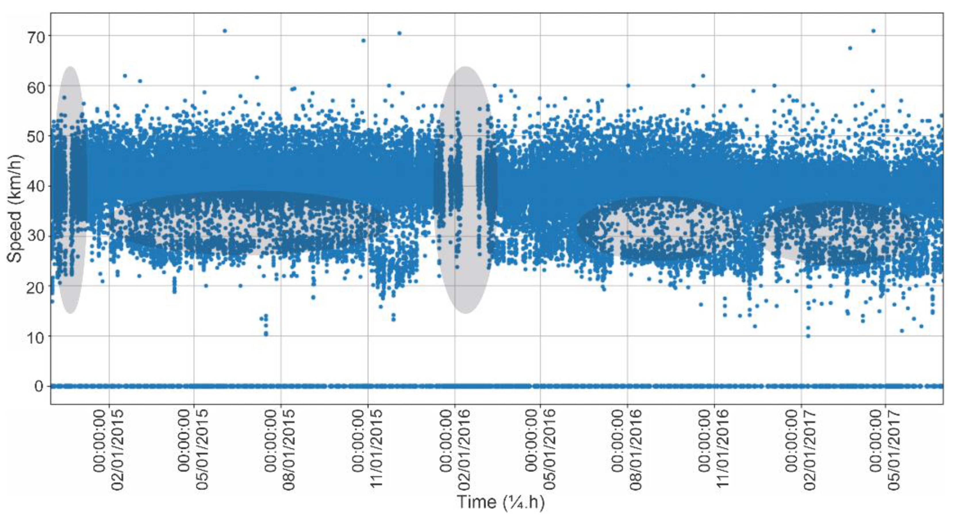
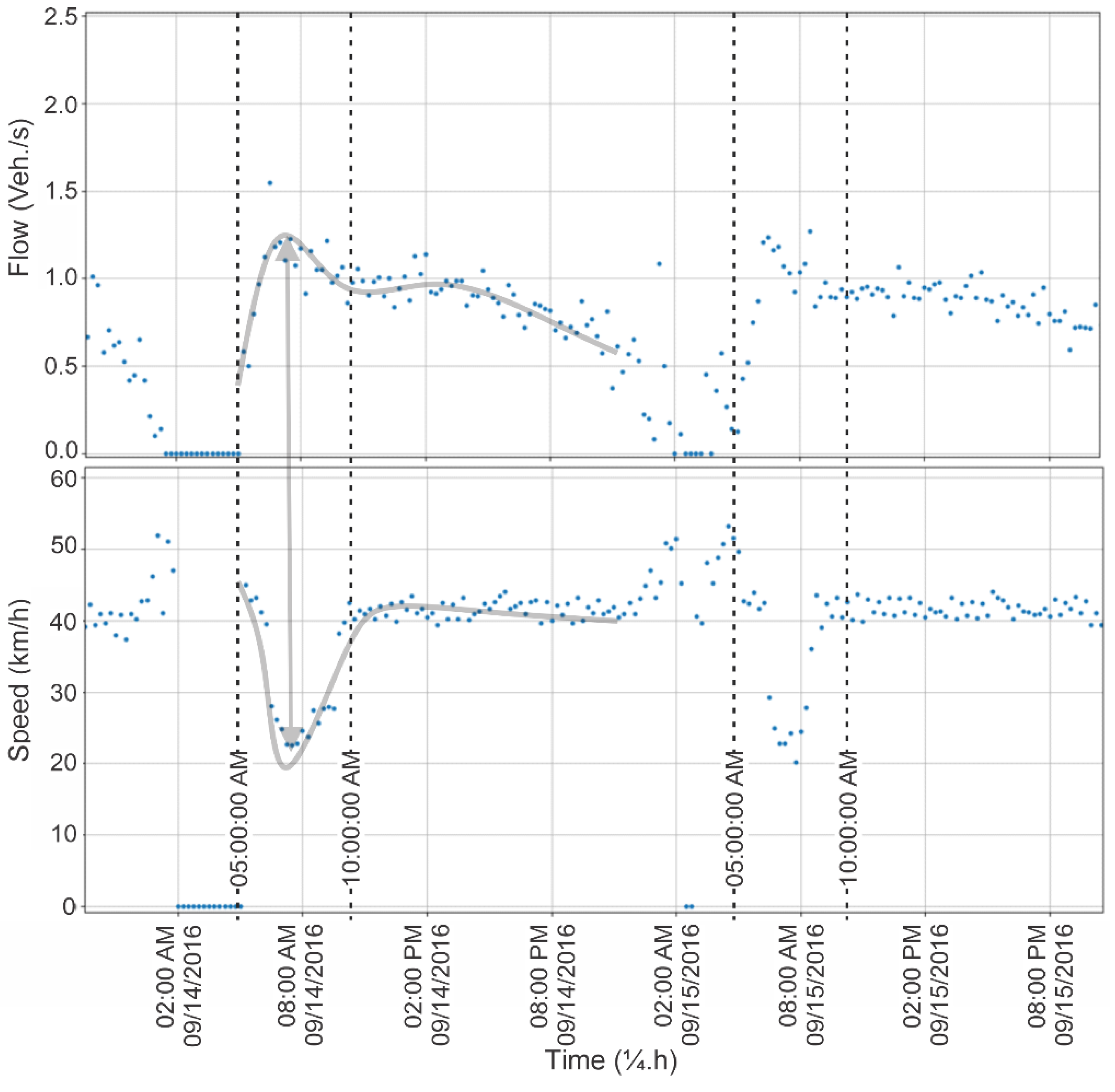
Thus, taking the RSI033 detector as an example, discontinuities in data collection can be observed, characterized by the interruption of the time series and irregularities in the velocity spectrum, as indicated by gaps between successive records on the same day. In the graph shown in Figure 4, both interruptions and irregularities can be identified over the 31 months of observations.

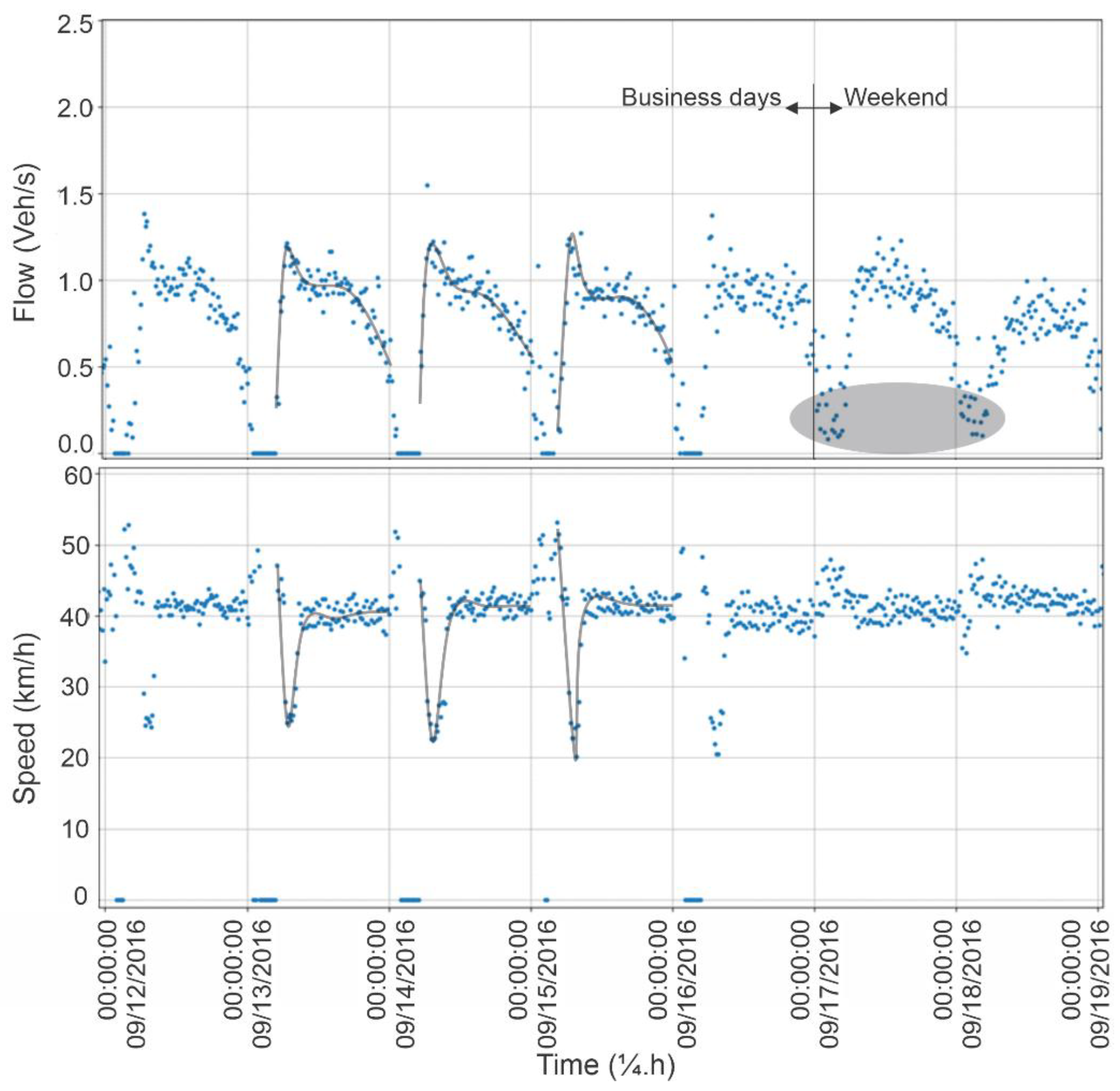
The preliminary analysis was performed in 15 min intervals. In this analysis, the traffic flow behavior varied during the week, between normal working days and rest days, typically weekends and holidays. This difference can be seen in both Figure 5 and Figure 6, in which the graphs of vehicle speeds and traffic flows were superimposed according to two different time scales: one weekly and one daily, respectively.

On Saturdays and Sundays, traffic flow appears before 05:00. It is less intense and grows more evenly distributed during the morning period, without major variations or congestion throughout the day. Consequently, low speeds do not occur on these days, as they do from Monday to Friday, when the pattern of behavior and the relationship between traffic flow and vehicle speed changes substantially.

Under the effect of the proximity of the weekend, traffic behavior on Monday and Friday is different from that on Tuesday, Wednesday, and Thursday. Traffic flow still starts before 05:00, probably because drivers are still returning from Sunday entertainment or leaving early to avoid congestion on the way to work in order to enjoy some after-hours fun on Friday. However, an inversely proportional relationship arises between traffic flow and vehicle speeds between 05:00 and 10:00, which does not happen on weekends. In this interval, traffic flow starts to increase, and proportionally, vehicle speeds start to decrease.

This inversely proportional behavior between traffic flow and vehicle speeds continues on Tuesday, Wednesday, and Thursday, but no flow occurs before 05:00. Flow increases; speeds decrease, and as this relationship intensifies over time, the flow and speed reach their maximum and minimum peaks, respectively. These peaks are inverse but coincident in time and occur before 08:00. On these sampled days, traffic flow reached practically 1.25 vehicles per second in all three lanes, i.e., 1500 vehicles per hour per lane while vehicle speeds were close to 20 km/h, indicating that congestion possibly occurred on the approach to the RSI033 detector.

Therefore, based on this preliminary analysis, the time intervals between 06:00 a.m. and 08:00 a.m. on Tuesday, Wednesday, and Thursday mornings exhibited continuous traffic flow gradients from lowest to the highest, going through saturation flow on the main road and then entering a free and stable regime. Therefore, the data recorded between 06:00 a.m. and 08:00 a.m. on business days in May and June of the year 2016 were selected to develop the present study.

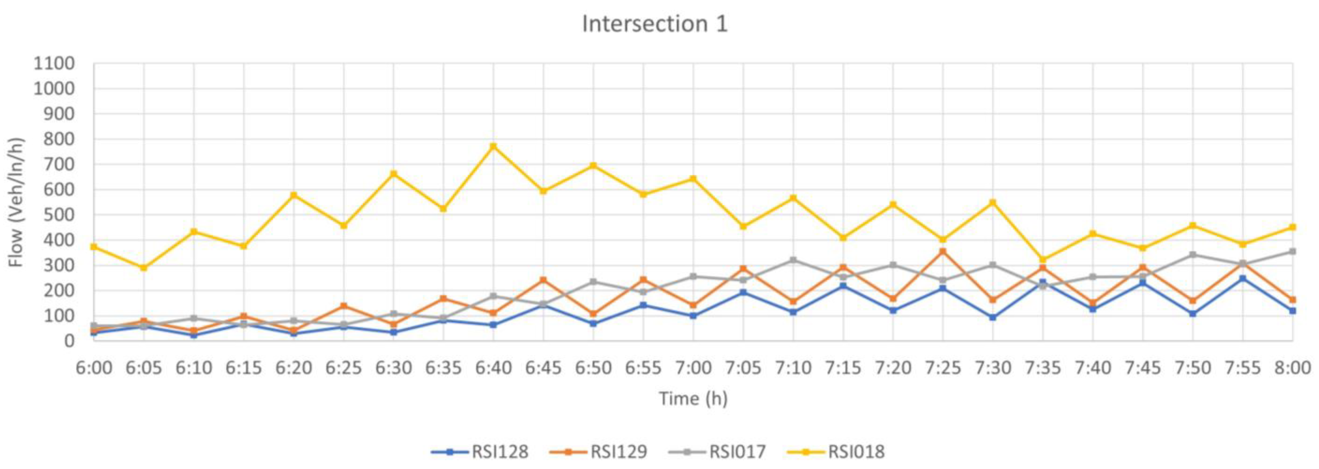
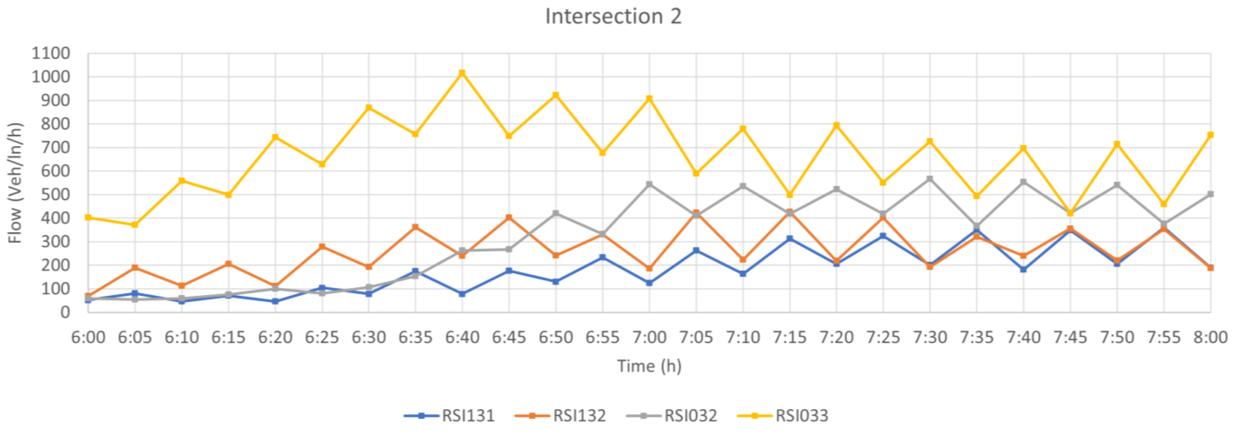
The graphs in Figure 7 and Figure 8 present the average traffic flow behaviors measured in 5 min intervals for the four approaches at each of the intersections during the 06:00 a.m. and 08:00 a.m. period on business days in May and June 2016. In this analysis, the average flow at the approaches of the two intersections show an upward trend for this time interval. In particular, the flow behavior lines based on the RSI018 and RSI033 detector measurements, respectively at intersections 1 and 2, show considerably higher traffic flow values than those at the other approaches. Moreover, the flow grows in the direction from intersection 1 to intersection 2 and reaches peak values at 06:40 a.m.

3.3. Modeling

To meet the objective of this research, the proposed model was developed based on the premise that each direction of an intersection is an element. Consequently, each intersection is composed of two elements. Then, since a traffic light can only be open or closed, the green signal time of one direction is the same for the opposite direction in the same element, and the green time of one element was taken as the red time of the other element of the same intersection.

Flow was calculated at each intersection element according to the number of vehicles passing in each lane per traffic direction and time unit within the green signal interval. To evaluate the extent of the traffic flow, it was assumed that as long as there was traffic flow in one direction, the traffic light was open at that element, and if there was no flow there, the flow in the other direction was tested in the same time interval. When confirmed, the flow was counted, and it was then deduced that the signal was closed at the previous element. The resulting test times were validated against the data reported by the local traffic authority.

Accordingly, once it was confirmed that the traffic light was green, the number of vehicles was counted within the evaluated interval. Then, the flow was calculated by the ratio between the number of vehicles and the time difference between the first and the last vehicle in the interval. The minimum phase verification time was set as equal to a minimum green time of 30 s although the developed algorithm allows any variation of this verification time. After this analysis and verification process, each calculated traffic flow was recorded.

Despite the possibilities of assuming other more typical states of a network, such as queue length, vehicle speed, and green or red-light time or a combination of them, an alternative state to characterize the traffic network, i.e., vehicle flow, was chosen to optimize the model.

3.4. Neural Network Selection

It must be added once more that the developed model in this work is based on the Deep Reinforcement Learning algorithm [23]. Complementarily, the work by [30] provides a good description of Deep Reinforcement Learning. Therefore, only the main structures applied to the implemented Deep Reinforcement Learning algorithm are next described, avoiding replicating what was already presented by [29].

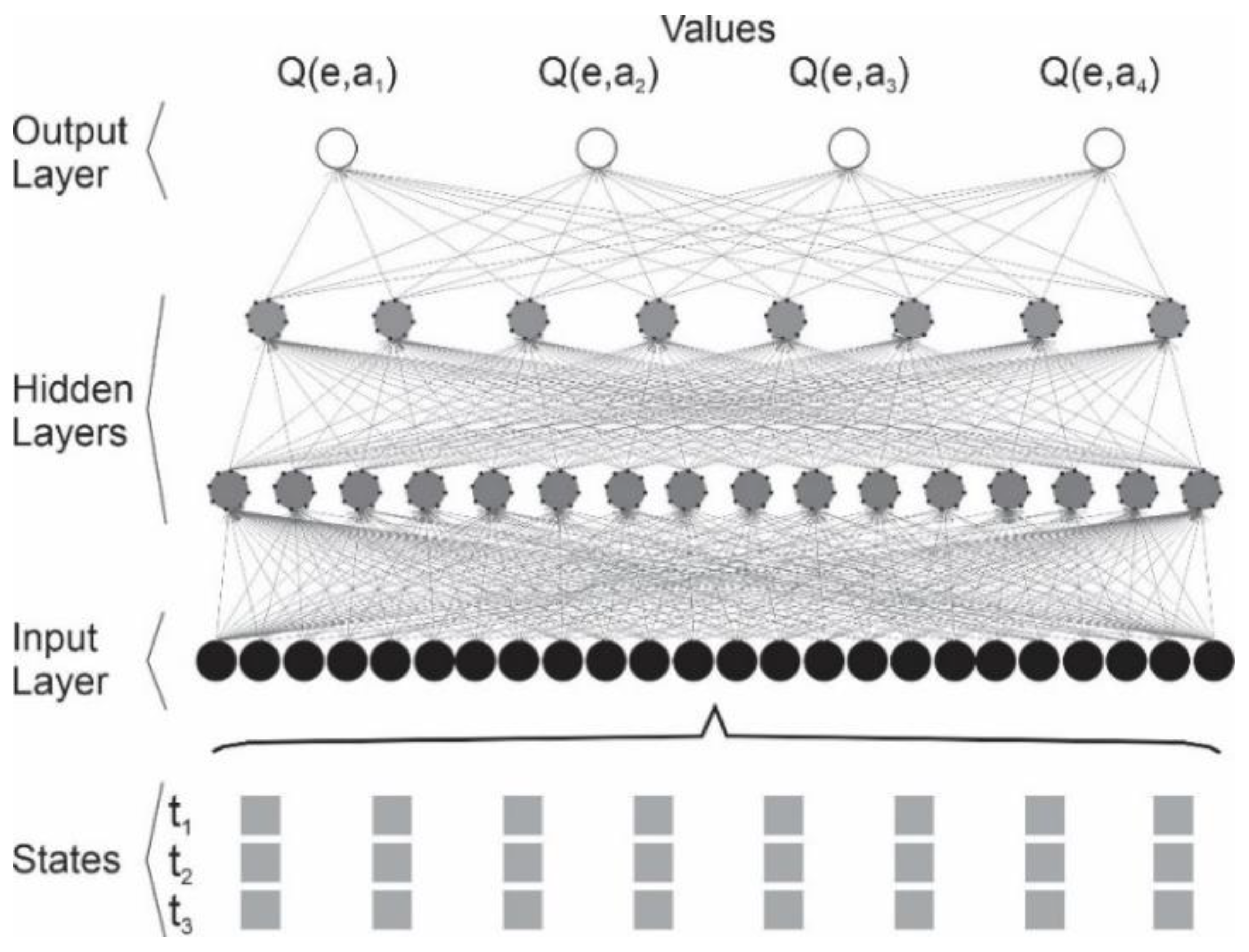
For the proposed model, a neural network with four layers was employed, including an input layer, two hidden layers, and an output layer. Since the model integrates two intersections with four-way flow measurements, and the three most recent measurements were taken as a sample to train the network, there were 24 neurons in the input layer. Then, the second and third layers, activated by a sigmoid function, were structured with 16 and 8 neurons, respectively. Then, since each intersection has one element for each direction, the output layer was designed with four neurons, one neuron for each element. Figure 9 presents the architecture of the neural network employed in the study model.

Next, the reward for the traffic signal actions was defined by two distinct portions, one local and one interlocal. While the local reward portion maximizes traffic flow in all directions of each intersection, the interlocal reward maximizes traffic flow only in the direction between the two intersections. Equation (1) details this total reward (r_t), where n is the intersection ID, and i is the travel lane of the roadway.

$$r_t={\displaystyle \sum }_{i,n}^{\begin{array}{c}i=1,2,3\\ n=1, 2\end{array}}\left\{\stackrel{local}{\overbrace{max\left[f_{i_n}^{\left(a\to b\right)};f_{i_n}^{\left(b\to a\right)}\right]+max\left[f_{i_n}^{\left(c\to d\right)};f_{i_n}^{\left(d\to c\right)}\right]}}+\stackrel{interlocal}{\overbrace{max\left[f_{i_1}^{\left(b\to a\right)};f_{i_2}^{\left(a\to b\right)}\right]}}\right\}$$

(1)

3.5. Evaluating the Results

The adapted traffic signal timing plans that resulted from the application of this deep reinforcement learning-based model were used to simulate traffic flow control during several working days in the interval from 06:00 a.m. to 08:00 a.m. Similar simulations were performed with the pre-existing traffic signal timing plan with the same collected traffic flows. Both simulations were performed using the VISSIM traffic microsimulation software program [31].

The performance of the proposed methodology was evaluated by comparing the results of the two simulations. Several performance parameters were measured and compared, especially those concerning delay, speed, and queue length.

4. Results and Discussion

The methodology produced intelligent traffic signal plans aimed at adapting to the actual demand conditions triggered by the traffic flow present at the approaches to the network intersections. As an example,

Table 1. Extract of the optimized traffic signal timing plan for each intersection in the network.

Route:	Arterial
Intersection:	1	2	1	2	1	2
Time	14 June 2016		15 June 2016		16 June 2016
06:35:19	True	False	True	False	False	True
06:35:29	True	False	False	True	False	True
06:35:39	False	True	False	True	False	True
06:35:49	False	True	False	True	True	True
06:35:59	False	True	True	True	True	True
06:36:09	True	False	True	True	True	True
06:36:19	True	False	True	True	False	True
06:36:29	True	False	False	True	False	True
06:36:39	False	True	False	True	False	True
06:36:49	False	True	False	True	True	False
06:36:59	False	True	True	True	True	False
06:37:09	True	True	True	True	True	False
06:37:19	True	True	True	True	True	False
06:37:29	True	True	True	True	True	False
06:37:39	True	True	True	True	False	True
06:37:49	True	True	False	True	False	True
06:37:59	True	True	False	True	False	True
06:38:09	False	True	False	True	True	False
06:38:19	False	True	True	False	True	False
06:38:29	False	True	True	False	True	False
06:38:39	True	False	True	False	False	True
06:38:49	True	False	False	True	False	True
06:38:59	True	False	False	True	False	True

partially describes the resulting intelligent traffic signal timing plan through an extract of the actions taken by the model between 06:35 a.m. and 06:39 a.m. for three working days in the middle of the month of June 2016. The table shows that actions are decided every 10 s with a minimum interval of 30 s for them to be effectively adopted. It is also evident that there is no regularity between decisions taken at equal times between consecutive days nor within the same day, even if they are taken at immediately successive times. Furthermore, different decisions are made to control different intersections. When these decisions are true, they are graphed with the color green to represent the green signal. Otherwise, they are graphed with red color to represent the red signal when they are false.

Furthermore, it was necessary to evaluate whether the intelligent traffic signal timing plans that resulted from the methodology proposed by this work met the objective of adapting to the actual conditions of demand caused by traffic flow. Therefore, as pointed out earlier, these plans were employed in microsimulations to control the traffic flows collected in the network in this study. The same number of microsimulations was performed by replacing only the intelligent traffic signal timing plans with the pre-existing traffic signal timing plans. In each microsimulation, VISSIM tracked and measured network performance, queue, and delay parameters.

Table 2. Network performance parameters obtained from traffic control with the intelligent traffic signal timing plan, according to microsimulations.

Parameters	Average Delay (s/veh)	Average Speed (km/h)	Average Delay (s/veh)	Average Speed (km/h)
Intervals	18 May 2016		15 June 2016
0–300 s	16.52	41.35	17.05	41.18
300–600 s	17.32	40.49	19.37	39.50
600–900 s	14.28	42.24	18.37	40.41
900–1200 s	23.13	37.93	22.82	38.21
1200–1500 s	19.93	39.76	20.65	39.23
1500–1800 s	22.01	37.84	26.05	36.63
1800–2100 s	21.33	38.73	20.13	39.17
2100–2400 s	34.72	32.74	32.49	33.91
2400–2700 s	30.72	34.21	29.49	35.16
2700–3000 s	33.08	33.42	34.52	33.51
3000–3300 s	28.19	35.44	28.41	35.15
3300–3600 s	31.56	34.17	33.74	33.39

highlights two of the network performance parameters—average delay and average speed—as examples.

For the purposes of evaluation and presentation of these results, they were later compared with the results of the same parameters obtained through other microsimulations performed with the pre-existing traffic signal timing plan. Thus,

Table 3. Improvements obtained by the adapted traffic signal plans compared to the pre-existing plans, according to the results of the simulations performed between 06:00 a.m. and 07:00 a.m.

PARAMETERS	SIMULATIONS
	17 May 2016	18 May 2016	19 May 2016	14 June 2016	15 June 2016	16 May 2016	Mean
NETWORK PERFORMANCE
Average delay	−34.39%	−20.59%	−32.32%	−26.69%	−28.46%	−27.94%	−28.40%
Total delay	−35.03%	−19.23%	−30.90%	−29.01%	−27.42%	−28.67%	−28.38%
Average speed	11.11%	6.78%	10.48%	8.54%	9.96%	9.45%	9.39%
Travel total time	−13.58%	−6.78%	−11.33%	−11.35%	−10.84%	−10.58%	−10.74%
Total vehicles in network	−16.67%	−9.49%	−12.39%	−15.65%	−15.74%	−16.31%	−14.37%
QUEUES
Queue length	−54.36%	−25.79%	−42.44%	−46.95%	−42.27%	−43.19%	−42.50%
Maximum queue length	−40.20%	−21.65%	−34.44%	−40.16%	−33.29%	−37.70%	−34.57%

and

Table 4. Improvements obtained by the adapted traffic signal plans compared to the pre-existing plans, according to the results of the simulations performed between 07:00 and 08:00 a.m.

PARAMETERS	SIMULATIONS
	17 May 2016	18 May 2016	19 May 2016	14 June 2016	15 June 2016	16 May 2016	Mean
NETWORK PERFORMANCE
Average delay	−31.14%	−19.52%	−31.43%	−30.95%	−22.28%	−35.08%	−28.40%
Total delay	−32.84%	−20.26%	−34.18%	−33.68%	−23.05%	−36.81%	−30.14%
Average speed	8.70%	5.70%	8.82%	9.07%	5.85%	9.82%	8.00%
Travel total time	−10.15%	−5.91%	−9.83%	−9.48%	−7.59%	−10.50%	−8.91%
Total vehicles in network	−12.49%	−6.84%	−10.17%	−10.62%	−5.70%	−10.11%	−9.32%
QUEUES
Queue length	−41.02%	−26.22%	−42.20%	−41.44%	−30.71%	−45.81%	−37.90%
Maximum queue length	−32.69%	−23.78%	−30.35%	−29.94%	−22.63%	−35.14%	−29.09%

present the percent improvements of the parameters measured by the simulator from the ratio between the results achieved by the model in this study based on deep reinforcement learning and the traditional deterministic model used by the local traffic authority.

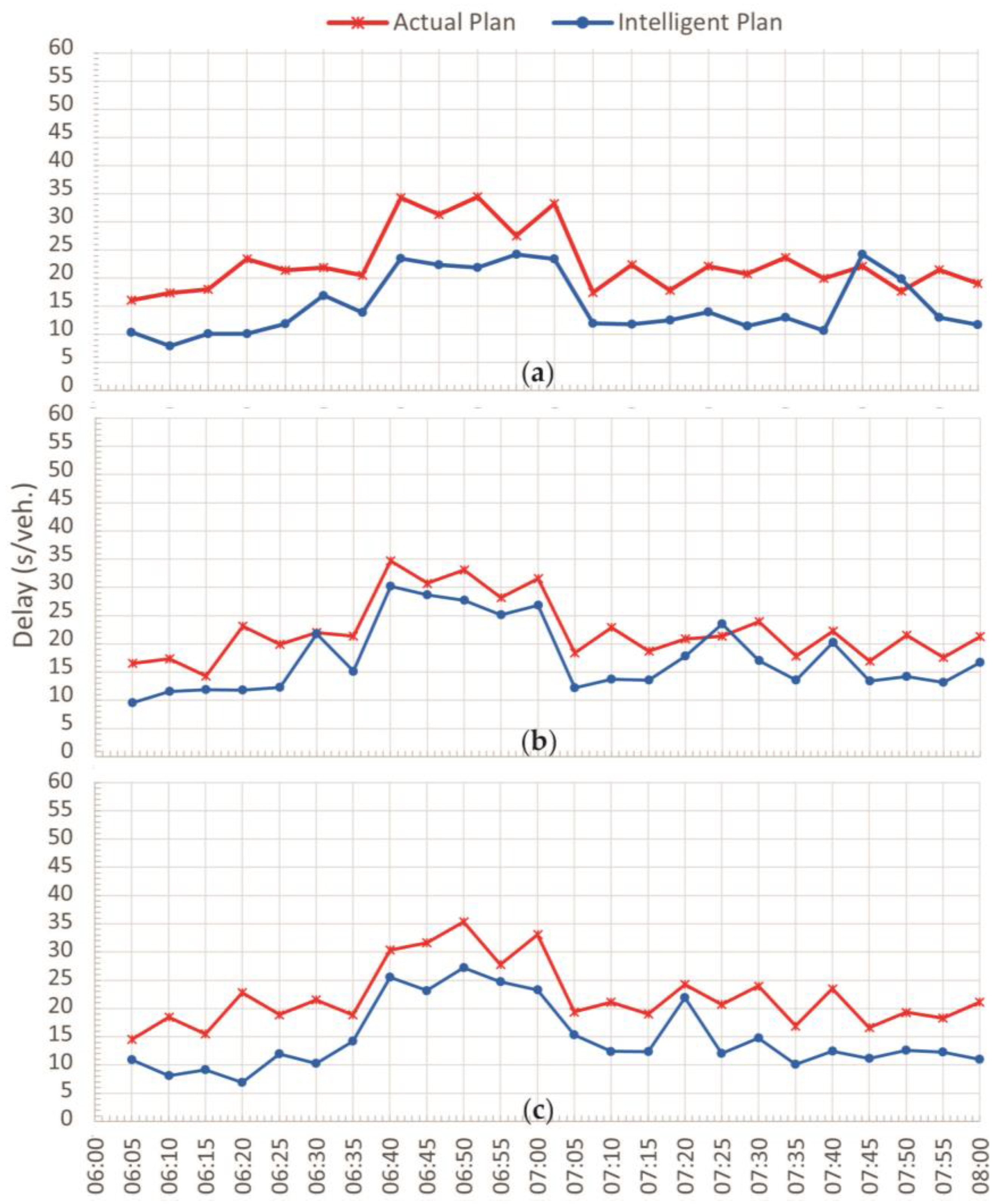
The percentages of improvement of the parameters that were generated by means of the methodology developed in this study should be interpreted as appropriate whenever the average speed in the network increases or the other recorded parameters decrease, including the average delay in the network and the length of queues at traffic light approaches. Figure 10 compares the average network delays simulated from the local traffic authority traffic signal plan and the intelligent traffic signal plans produced by the model proposed in this paper. In this sense, negative percentages represent a reduction and positive percentages represent an increase in the ratio between the parameters. When these percentages are graphed with the color blue or red, they will be respectively adequate or inadequate according to the desired behavior for the parameter.

It is worth noting that the simulation averages show reductions of 28% for network delays, as well as an increase of more than 9% in the average network speed. Queue lengths were reduced by more than 42% and maximum queue lengths by more than 34%. The simulations performed between 07:00 a.m. and 08:00 a.m. yielded slightly lower results compared to those obtained earlier in the interval between 06:00 a.m. and 07:00 a.m. The exceptions are the total network delay and the average delay. However, the orders of magnitude of the percentages of reduction or increase are similar in the two intervals.

It is also important to compare the results obtained in this work with the ones applied, for instance, by the main adaptive real-time traffic control systems in use in the USA [19].

Table 5. Comparisons of the performances of the proposed model and the main adaptive traffic control systems already in use in the USA.

Systems of Adaptative Traffic Control	Performance
	Travel Times	Delays	Stops
Developed Model	−13.6% to −5.9%	−36.8% to −19.2%	−26.1% to +9.3%
SCOOTS	−29.0% to −5.0%	−28.0% to −2.0%	−32.0% to −17.0%
SCATS	−20.0% to −0%	−19.0% to +3.0%	−24.0% to +5.0%
OPAC	−26.0% to +10.0%	-	−55.0% to 0%
RHODES	−7.0% to +4.0%	−19.0% to −2.0%	-
ACS	−12.0% to +7.0%	−38.0% to +2.0%	−35.0% to −28.0%

presents these comparisons. When analyzing Table 5, one can see that the developed model achieves quite reasonable results when compared with the other models. In particular, the evaluated delays by the developed model in this research were very good ones ranging from −36.8% to −19.2%, Further studies should evaluate ways to improve the ranges of the obtained stops even though the obtained results by the Deep Q-learning method were quite similar with the SCATS tool.

When analyzing the results presented in Figure 10, it must be added that the developed intelligent model in this work maximizes the traffic flow in the network. It did not consider any of the other possible traffic states, nor did it restrict network performance parameters. It was then observed that on 17 May 2016, at 7:40 a.m. and 7:45 a.m., there were punctual and sudden increases in the flow in the arterials, and then, the applied Deep Q-learning model tried to maximize the flow on those arterials. Therefore, there was a decrease in the flow in the main road and, consequently, an increase in the average delay of the network. Quite interestingly, the same occurred on 18 May 2016 at 7:25 a.m. where there was a sudden and punctual increase in arterial flows at that time. Moreover, when analyzing in detail the data set, it was showed that one of the sensors, the RSI017 one, failed at 7:40 a.m. on 17 May 2016 since it did not register any flow at that time. This fact can certainly have affected even more the work of the Deep Q-learning model since it considered a 0 (zero) flow for that sensor when applying its algorithm.

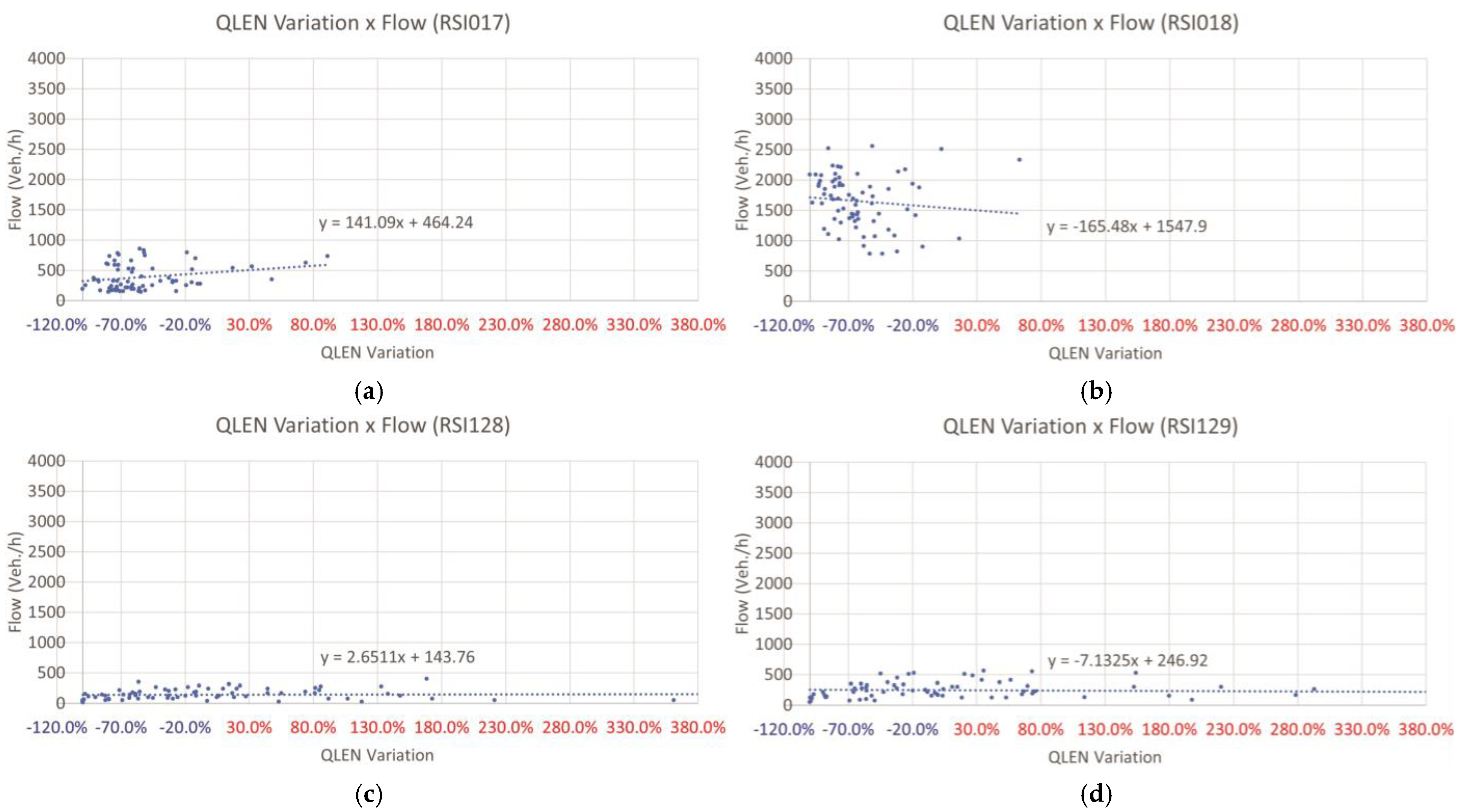
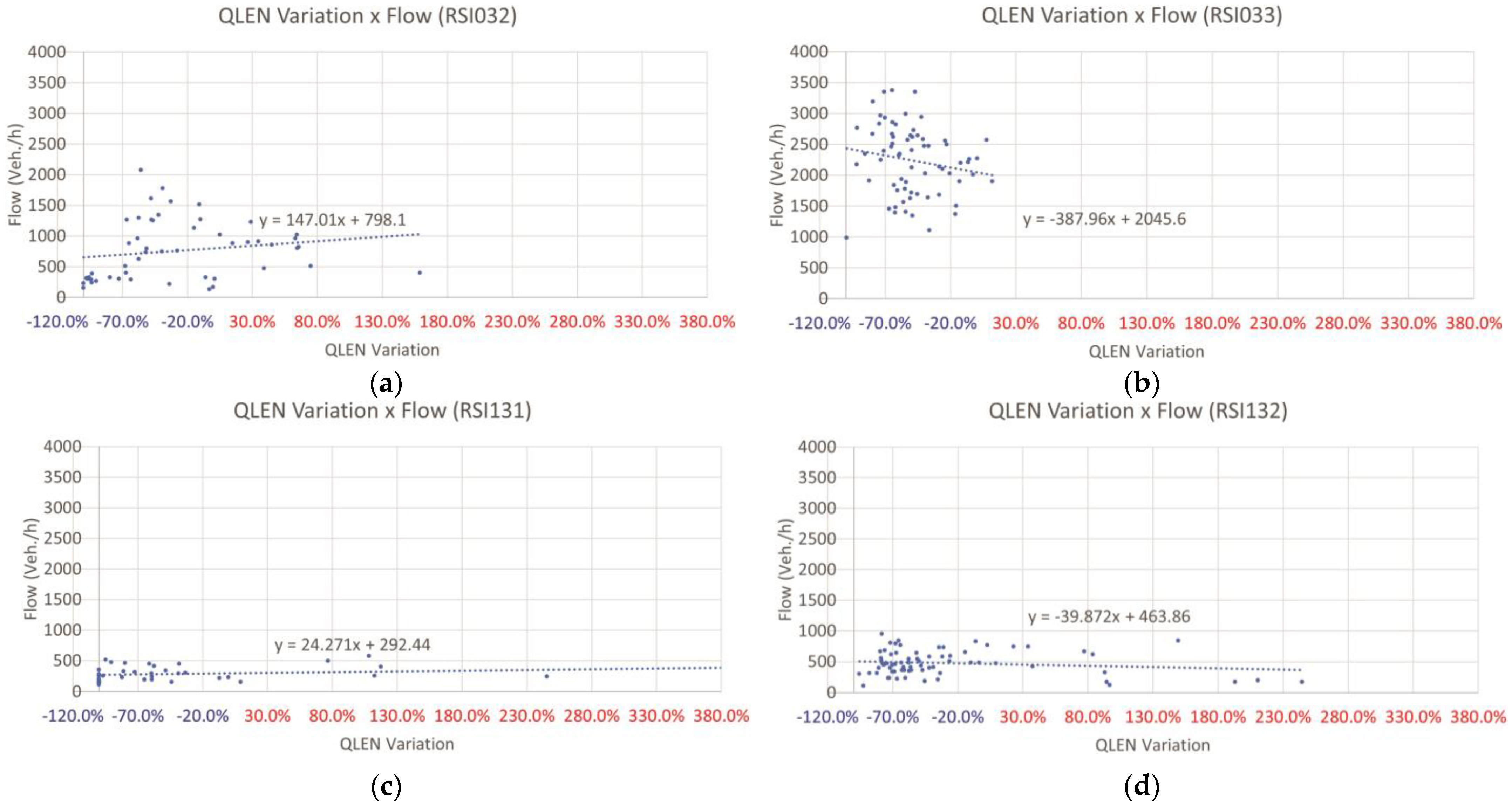
We sought to evaluate the results obtained individually at intersections and at traffic light approaches in order to add value to this analysis and considering that the reward for the actions integrated two portions, both a local portion referring to the optimization of intersections and an interlocal portion referring to the optimization between intersections. In this sense, the queue length was chosen to present the results of this approach.

Therefore, as described above, the ratios between the results obtained from each of the traffic signal timing plans, the intelligent one and the pre-existing one, were measured, and the criterion for evaluating the appropriateness of the negative and positive percentages of these ratios in relation to the goal was maintained. It is worth noting, in the case of the queues, that the negative percentages indicate more appropriate results, because they demonstrate a reduction in their lengths.

These percentages adopted to express the variations in the parameters were correlated with the respective traffic flows in each of the approaches that make up the intersections of the network. Thus, it was possible to observe how the proposed approach reacts based on the increase or decrease in traffic flow in the network, at the intersections and approaches. Figure 11 and Figure 12 present these correlations for the network and for each of the intersections, respectively. Note that the linear regressions fitted to these correlations show negative angular coefficients, i.e., the model proposed here tends to cause a reduction in queue lengths relative to the usual condition subject to the control performed by the pre-existing traffic signal timing plan.

Given the application of this model based on deep reinforcement learning, the growth of queue lengths and maximum queue lengths tends to be smaller as traffic flows increase, as a result of the more efficient signal control provided by the signal timing plans adapted to the dynamic and real conditions of the traffic network studied.

An analogous procedure was subsequently applied for each approximation. The intersections were discretized to present the resulting behaviors of the queue lengths in each of their approximations. Figure 13 and Figure 14 highlight what happens to the queue lengths in the approaches that connect at each intersection. Isolating the results of the approaches, identified in the graphs by their inductive loop detector codes, it is evident that in the direction of the predominant flows that coincide with the arterial road, the signalized approaches in the direction of higher traffic demand (RSI018 and RSI033) have predominance over the approaches in the opposite direction, with less vehicle traffic demand.

In the face of higher flows in one direction, the respective queue lengths are reduced considerably while the queue lengths in the opposite direction are sacrificed to the extent that the method accepts slight increases in queue lengths in that direction when facing lower flows. The angular coefficients of the linear regressions define a rate of reduction of this parameter when negative or increase when positive. In the other direction of the intersections, on which the collector roads are aligned, the flows are significantly lower. Therefore, although the effect of the model seems smaller, the same decision is made to reduce queue lengths in the direction with higher flows to the detriment of a small increase in queues in the opposite direction, which has lower traffic demand.

Finally, the presented results can be compared with previous works including the ones by [32,33]. These works show advantages to the traffic controller field being based on the established techniques of Dynamic Programming and Reinforcement Learning. Reference [32] developed a real-time traffic optimization model implementing the dynamic programming approach such as the Rhodes technique. Moreover, [33] proposed an urban traffic controller combining a Reinforcement Learning algorithm, the Distributed W-Learning one, jointly with the Deep Reinforcement Learning algorithm, the Deep Q-Network one.

The models by [32,33] were implemented in an urban traffic network comparing their performances to the ones of the Rhodes approach and the SCOOT system (Split Cycle Offset Optimization Technique—SCOOT), respectively. Reference [32] applied a flow data obtained by a traffic prediction model, and [33] used statistical data from a government survey.

When comparing the results in [32] with the ones of the Rhodes method, it was observed that [32] obtained an improvement of 15.1% of the average traffic delay. Moreover, when comparing the work by [33] with the SCOOT approach, an improvement of 17.2% in the stops was evaluated.

Regarding the already mentioned parameters of traffic delay and the number of stops, the work developed in this research can also be compared with the Rhodes and the SCOOT ones. The developed model can achieve, on average, 19.5% less delays when compared with the Rhodes one, but it achieves 21% more stops when it is compared with the SCOOT approach. Nevertheless, when the measured parameter is the average traffic delay, the implemented model achieves 15.3% less delays than the ones obtained by the SCOOT technique.

The Deep Reinforcement Learning implemented model shows then, in general, valuable improvements. It is important to mention that this work applied a real data set. Therefore, the input data set was neither obtained by a prediction model nor by a government survey. This pattern of the used data set suggests the robustness of the applied model, since a real data set can have not only missing data due to the failure of the sensors but also huge deviations because of the occurrence of accidents, for instance [34]. Further studies can also be carried out to evaluate ways to decrease the number of stops of the applied model including the minimum time for a traffic light phase and the batch size to train the ANN.

5. Conclusions and Recommendations

The model based on deep reinforcement learning proposed in this paper holds similarities with the work of [23]. However, the introduction of a new expression for calculating the total reward and the use of traffic flow as its maximization parameter have added considerable advances to the way of controlling urban traffic through traffic signal timing plans adapted to real flow conditions.

Regardless of the dimension observed, whether in the network, the intersection, or the approach, the results obtained are very promising. In relation to the pre-existing condition, all of the parameters of the traffic network were reduced by the application of the proposed model. In general, average speeds in the network increased by 9%, and delays and queue lengths were reduced by more than 28% and 42% in the period of highest traffic demand, respectively. In situations where traffic demand was lower, the percentages of improvement were also significant and very close to the previous percentages, demonstrating that the configuration defined to determine the total reward added value to the proposed model.

The graphs of the arterial road approaches, identified by the detector codes named RSI017, RSI018, RSI032, and RSI033, showed that the proposed approach sacrifices the directions with lower traffic demand (RSI017 and RSI032) by increasing the length of queues in order to improve fluidity in the opposite direction, which has a higher traffic flow (RSI018 and RSI033). This prevents increasing queues at these approaches, improving network performance in light of dynamic, real-world conditions. Furthermore, analysis of the graphs of the approaches to the collector roads, identified by the detector codes RSI128, RSI129, RSI131, and RSI132, showed that this sacrifice and benefit behavior between smaller and larger flow directions does not only occur in the presence of high traffic demands but also in the presence of low flow.

This model therefore improves network performance for a broad spectrum of traffic flows, regardless of their magnitude, because it is able to perceive and decide at both high and low traffic flow levels. Based on these same results, the decisions taken by this approach to privilege directions with higher demand do not hinder traffic in the other directions guaranteeing an increase in the performance at the approaches, in isolation or not.

The method proposed by this research is independent of a traffic model, providing good results in situations of greater or lesser demand on the transit network. Accordingly, this method is able to perceive the variations in the flow and decide which direction or direction should be favored over the others. This ensures better traffic conditions without jeopardizing any of the preferential directions, benefiting both the intersections and the network, for all the parameters observed.

Moreover, the proposed model demonstrated the ability to respond appropriately, controlling traffic even in the absence of traffic data, as shown in the 07:40 a.m. record on 17 June 2016, Figure 10. Since the applied algorithm deals with real-time traffic control, it is possible to assume that some sensors can fail at a given time. Therefore, further research should be carried out trying to mitigate these possible sensors failures when applying the developed tool.

Certainly, the use of data collected in the field has added validity to the application of the model, which is important due to the intrinsic behavior of real events and the consistency of the achieved results. However, it would be interesting to apply this new model to a larger data set without as many gaps in the time series, comparing once more the evaluated results with the ones obtained by market models.

In general, traffic data are not widely available in Brazil. Therefore, even though this research had access to a large database of flow, it was related to only two intersections. In the future, when a larger data set in a larger network becomes available, the developed model can then be applied to better evaluate its effectiveness. Further studies should also extrapolate the simulation environment based on this deep reinforcement learning method to an experimental network requiring optimization. One should then take into account the availability of inductive loop detectors in Brazil or in other countries, and the ease of using this model with real data independent of the collection source. Technological advances are also important to apply the proposed approach, due to the increasingly larger and more accessible computing power.

The development of smart cities and autonomous vehicles will make the smart road environment a reality allowing both the proper collection of flow data and its availability in real time. These facts will greatly benefit the Deep Reinforcement Learning models because of their simplicity and sensitivity to quick and unexpected changes.

As it was already stated, the developed model did not depend on a traffic model nor on several traffic parameters that are routinely calibrated. The presented model, which was a Deep Reinforcement Learning one, used only the real traffic flow data to define its state integrating two intersections in a network in a centralized way, which had not yet been done by previous research, to our knowledge.

Finally, it must also be added that one of the main contributions of this work is regarded to be the simplicity to implement it operationally due to the already available technologies. These technologies allow not only to count vehicles in real time but also the promptly availability of data to the various actors and entities of the Traffic System, especially with the development of smart cities.