Exploiting Low-Cost 3D Imagery for the Purposes of Detecting and Analyzing Pavement Distresses

Abstract

Road pavement conditions have significant impacts on safety, travel times, costs, and environmental effects. It is the responsibility of road agencies to ensure these conditions are kept in an acceptable state. To this end, agencies are tasked with implementing pavement management systems (PMSs) which effectively allocate resources towards maintenance and rehabilitation. These systems, however, require accurate data. Currently, most agencies rely on manual distress surveys and as a result, there is significant research into quick and low-cost pavement distress identification methods. Recent proposals have included the use of structure-from-motion techniques based on datasets from unmanned aerial vehicles (UAVs) and cameras, producing accurate 3D models and associated point clouds. The challenge with these datasets is then identifying and describing distresses. This paper focuses on utilizing images of pavement distresses in the city of Palermo, Italy produced by mobile phone cameras. The work aims at assessing the accuracy of using mobile phones for these surveys and also identifying strategies to segment generated 3D imagery by considering the use of algorithms for 3D Image segmentation to detect shapes from point clouds to enable measurement of physical parameters and severity assessment. Case studies are considered for pavement distresses defined by the measurement of the area affected such as different types of cracking and depressions. The use of mobile phones and the identification of these patterns on the 3D models provide further steps towards low-cost data acquisition and analysis for a PMS.

1. Introduction

1.1. The Need for Low-Cost Automated Pavement Distress Application

Road networks are key drivers towards the economic viability of a country. They provide movement for users, goods and services as well as providing access to social benefits for commuters [1]. Pavements represent a vital part of the road network, and it is imperative that they are kept in a suitable condition to avoid accidents and provide efficient access to road users. Road agencies are tasked with this responsibility and have to make critical decisions to develop road maintenance and rehabilitation strategies. However, globally it has been noted that there has been a growing reduction in budgetary allocations for these purposes [2,3].

To achieve suitable maintenance strategies, a pavement management system is commonly applied by road agencies. The pavement management system (PMS) is seen as the most common and effective system for crafting maintenance strategies and it can be characterized as one that optimizes road management to achieve the most effective use of financial resources given the needs of the road system [4]. The PMS integrates a wide range of functions to give practitioners a decision support system for effective planning for the large investments required for pavements [5]. However, a PMS is reliant on high-quality road condition data. The acquisition of these data can, in turn, be very expensive, exhaustive, and time-intensive [6]. Given the already strained road agency budgets, this leads to many authorities not being able to implement an effective PMS as in many instances road condition surveys are manually carried out [7]. As a result of this, there has been a significant amount of research carried out to obtain new but accurate and low-cost methods of acquiring road condition data, specifically data on pavement distresses that are present within a network [8,9].

1.2. Background of Pavement Distress Detection Techniques

The most studied areas of techniques of detecting and analyzing pavement distresses are techniques involving laser-based systems and those involving imagery from cameras. There are several commercially available equipment that utilize laser technologies equipped to vehicles for the purpose of understanding road conditions. The laser crack measurement system (LCMS) [10] is the basis of many of these systems and relies on the use of high-performance lasers attached to a vehicle that measures the profile of the road, roughness and slope at a high resolution of 1 mm whilst producing 3D profiles of the pavement. There have also been the development of mobile laser-based systems and those employing light detection and ranging systems [11,12].

The systems based on lasers are generally thought to be the most accurate techniques for detection but they are also generally more expensive and this reduces the possibility of road agencies being able to utilize them [13]. There are also systems that incorporate both imagery and lasers to produce additional information on the road conditions [14,15].

Given the costs of the laser systems, the option of utilizing only imagery provides an attractive alternative as costs of camera systems are typically significantly cheaper. Camera-based systems usually include capturing images of the pavement surface followed by subsequent interpretation and analysis based on anomalies detected within the images. The interpretation can be done with the use of algorithms that process the images [16,17,18]. There is a wide array of image-based technologies that have been studied for the purpose of detection, classification and analysis of pavement distresses [19]. One particular low-cost image-based method is stereoscopic surveying including the use of photogrammetry and structure-from-motion. These techniques aim to recreate 3D models of the object being analyzed and recent work on this in the field of pavement distress detection has shown the accuracy of utilizing this method [20]. This field of research provides additional opportunities for the analysis of pavement distresses as accurately generated 3D models can provide critical metric information on the distress that can yield effective intervention strategies.

1.3. Using 3D Imagery to Detect and Analyze Pavement Distresses

Structure-from-motion (SfM) is a photogrammetric modelling technique utilized to replicate 3D models of objects. It is a low-cost method that employs the use of algorithms to reconstruct the object using simple 2D imagery [21]. Within the technique, overlapping images are typically taken around the object at different angles. Specific algorithms for image alignment and bundle adjustment are then applied to establish the object’s position in three-dimensional space [22]. Figure 1 showcases an example of a dataset obtained across a distressed asphaltic pavement section.

SfM techniques have generally been utilized in other fields such as architecture and archaeology for the preservation of artefacts and historical figures [23]. There have also been studies on asphalt pavements wherein the techniques were used for replicating road surfaces and their distresses [16,17] and other studies have considered using drones to carry out the process [24,25]. Previous works concluded that there was a lack of available industry tools to utilize the techniques [26]. However, new developments in processing power and algorithms have made it possible for application to pavement engineering [20]. Recent studies have shown the accuracy of models by comparing results to those from laser technologies [27]. This verification of accuracy is in line with typical photogrammetry accuracy development cases for buildings and other structures [28,29]. With the comparisons made to lasers, it was established that professional cameras are capable of carrying out the process. However, these cameras can still be quite expensive and establishing a pipeline using professional cameras still requires the procurement of the devices followed by subsequent training on their use by road agency staff. To this end, if a pipeline could be established using mobile phones then the process can be considered more operational and the potential for its use is accelerated. Therefore, whilst other studies have focused on using the techniques with drones and expensive cameras, this study aims to demonstrate the accuracy of using the techniques with mobile phones to generate 3D pavement distress models to help bridge this research gap and provide quantitative results on the accuracy of developing this mobile pipeline. Furthermore, whilst other studies have focused on simple metric analysis, using metric parameters typically recovered from distresses such as distress dimensions of length and width, the second goal of the study is to establish methods to critically evaluate the distress using segmentation and enhancement strategies. This provides therefore, a sectional analysis methodological point of view. By doing this, distresses can be easily isolated and at this point then the common metric evaluation can be done. To do these analyses, case studies utilizing different strategies and distresses are considered for specific distress types.

1.4. The Use of Image Segmentation in Pavement Condition Evaluations

Whilst it is useful to recreate the pavement distress with 3D imagery, it is also useful to identify features on these models. Image segmentation is considered for this. It is the process of dividing an image into smaller related segments for the purpose of analyzing and isolating particular features. With regards to pavements, the purpose of image segmentation would be to isolate pavement distresses in order to quickly pinpoint the location of the distress and also for analyzing the type of distress. There have been several attempts over the years to carry this task out utilizing different datasets. Studies have tried to extract useful features from drone image data [25], LIDAR point cloud data [30], Google street view image data [31], 3D laser profilers [32,33], 3D laser images [34] and normal 2D images [35]. There have also been attempts to utilize convolutional neural networks for the purpose of segmenting pavement images using annotated masks on the images [36].

There are challenges to the acquisition of these types of data sets and then also with regards to the processing power required to analyze them. To this end, this study focuses on the use of a low-cost image acquisition pipeline using mobile phones. Mobile imagery data has an advantage over drone data in that higher resolutions can be yielded given that distance to the object is smaller and also surveys can be made in areas where drone use is forbidden. When coupled with the SfM techniques, mobile imagery can be utilized to create point clouds of a distress and these point clouds can be segmented without excessive processing power. Point clouds have previously been classified to produce depth maps and smaller more useful models within the original model in other fields of study [37]. Generally, the process can function as depicted in Figure 2.

Given these factors, this study aims to generate depth maps and extract and isolate critical elements and sections from 3D models generated by imagery from mobile phones.

2. Materials and Methods

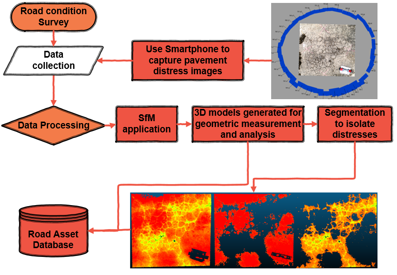
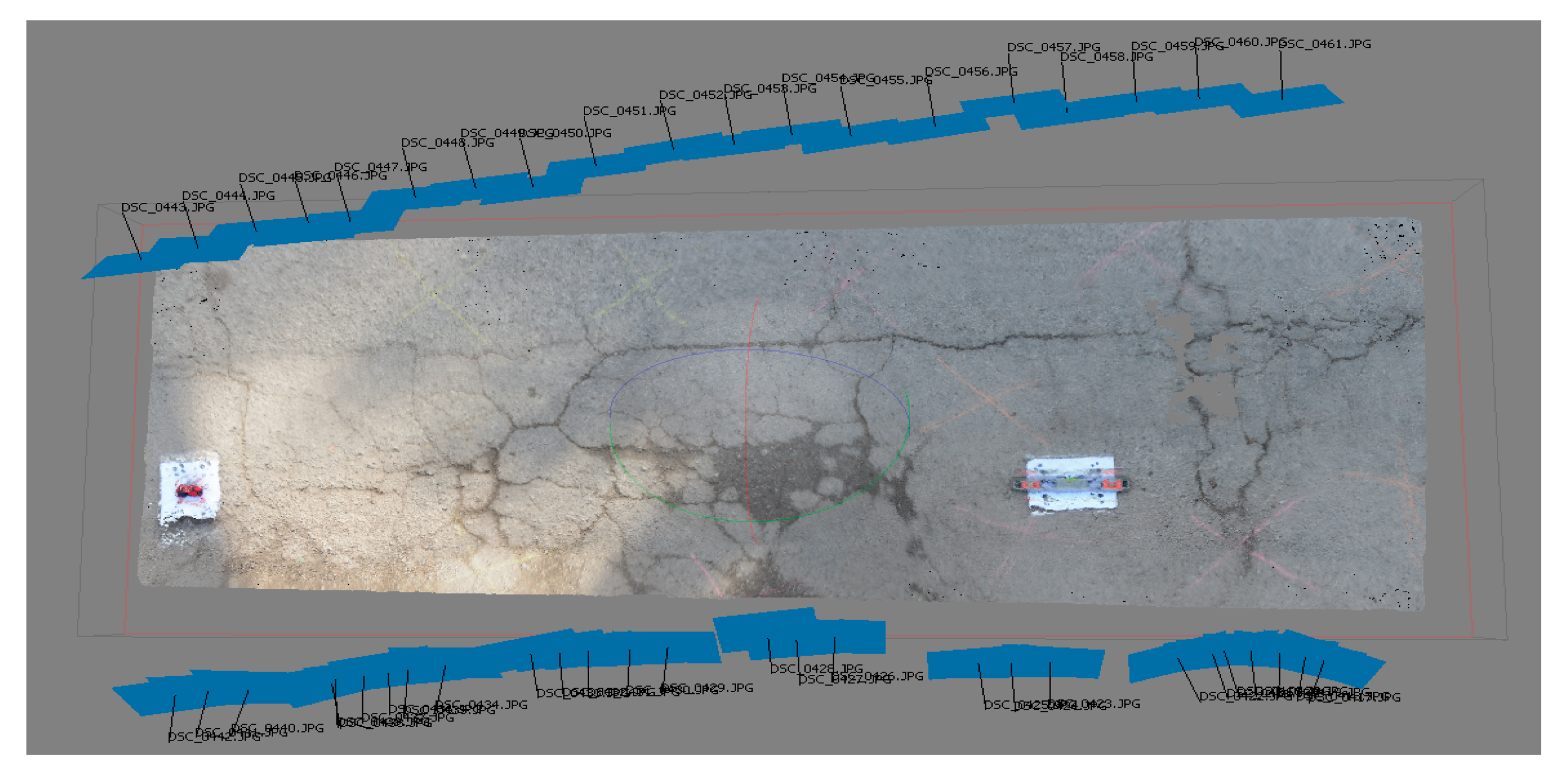
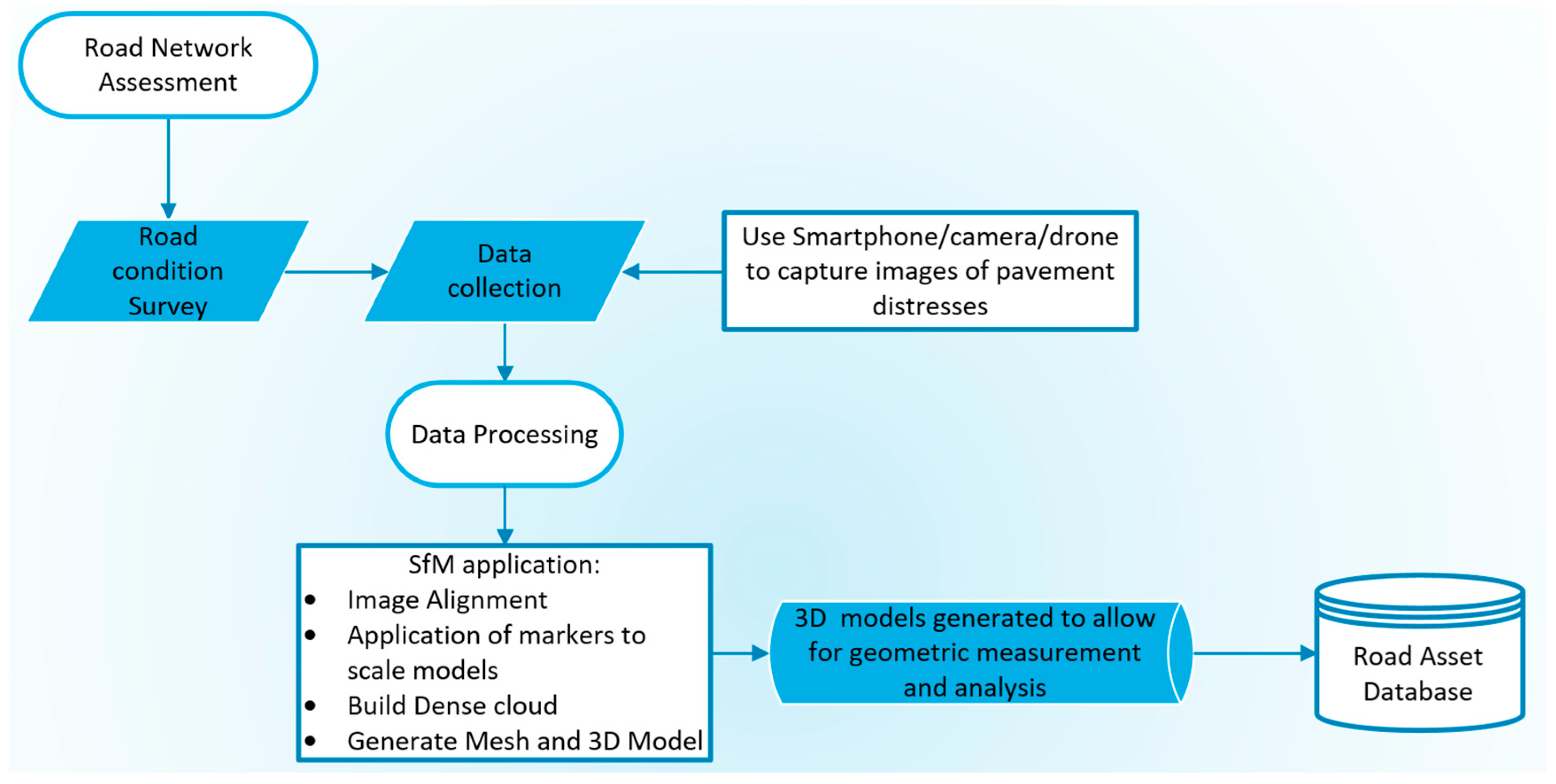
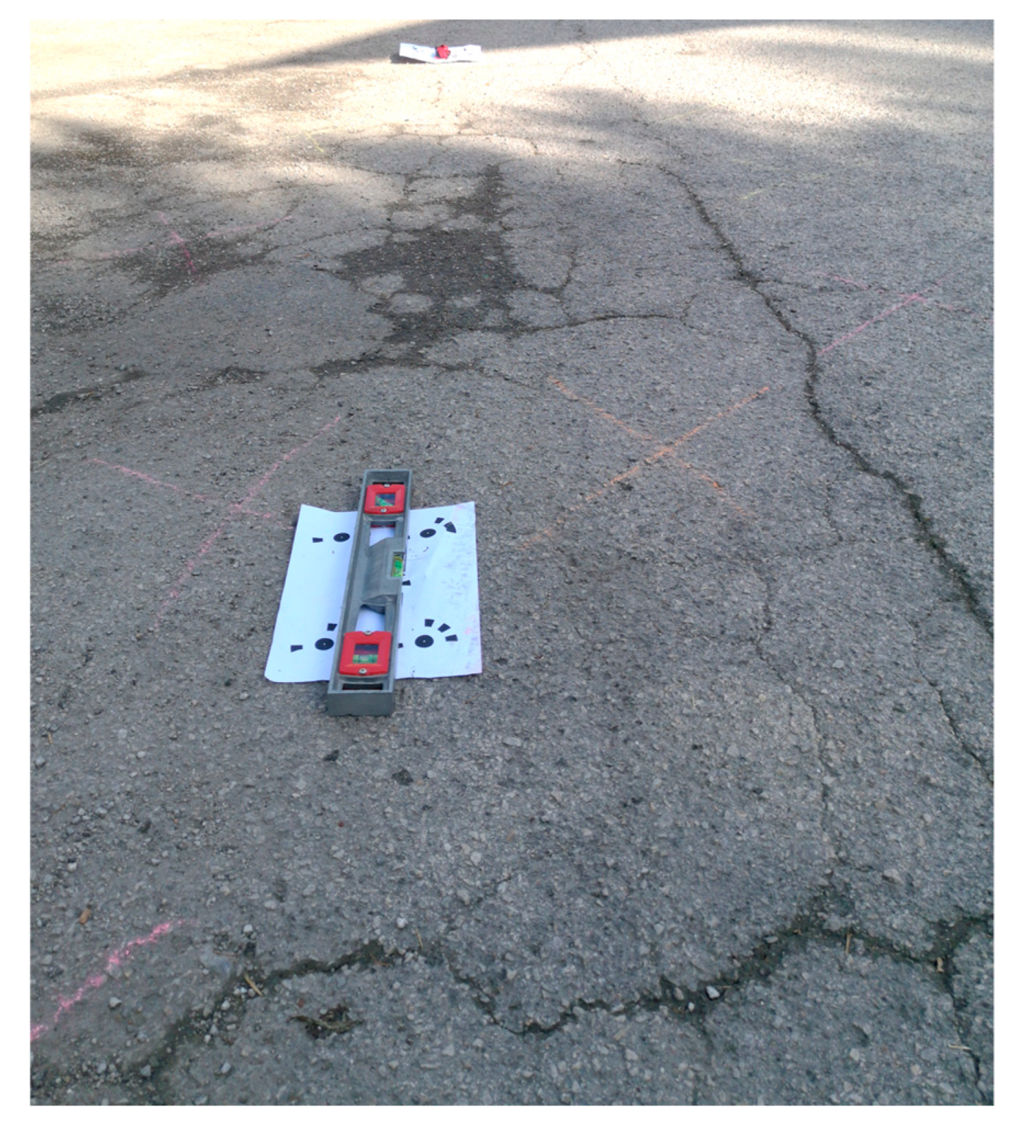
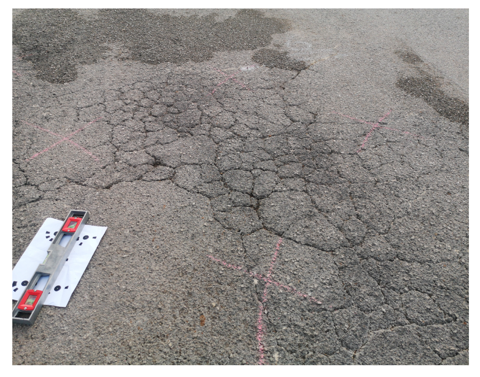
2.1. Structure-from-Motion Setup and Workflow

Whilst utilizing structure-from-motion techniques, the most critical parameter to be considered is the ground sampling distance (GSD). This is the typical parameter from which models are interpreted. It is a representation of the distance between two consecutive pixel centers, with respect to actual ground measurements. The GSD is considered as a representation of the smallest details that can be accurately observed on an image [38]. The smaller the value of the GSD, the greater the details that are measurable. This shows the importance of this value as it will dictate the resolution of the replicated models and thus the possible level of observable features. For the GSD, it has been demonstrated that the smallest visible details are two to three times the value of the GSD [39]. Generally, cracks and common distress are smaller than 0.01 m (10 mm) and with resolutions of 3mm these distresses can be accurately identified [40]. Therefore, the technique must be able to produce a resolution less than this. For typical 2D imagery used for detection, a 3 mm resolution is utilized [9]. Given that a detection of 3 mm which would be appropriate for pavement distresses, the GSD should be no greater than 1 mm. As a lower resolution would be better, a value of approximately 0.5 mm was sought after within this study. The GSD is related to specific parameters of the camera used and is given by Equation (1) below.

$$GSD = \frac{D \times p{x}_{size}}{f}$$

(1)

where D = object distance, ƒ = focal length, and px_size = pixel size (as defined by the ratio of the camera’s sensor height to the image height). The focal length and pixel size are attributes from the camera and the other parameters can be manipulated to produce an appropriate GSD. For the purpose of this study, a GSD of 0.5 mm was aimed for so the object distance was manipulated to ensure this value was obtained for the survey. Three devices were utilized for the surveys. A professional camera was used and two different common market mobile phones were used to test the accuracy of the technique using mobile phones. The camera was used as a control in the experiment. The specifications for these devices are given in

Table 1. Specifications of devices used for SfM surveys.

Device	Nikon D5200	Huawei P20 Pro	Samsung Galaxy S9
Camera resolution [Megapixel]	24	40	12
Image Size [pixel]	6000 × 4000	3648 × 2736	4032 × 1960
Focal length used [mm]	24	3.95	4.3

. Mobile phones were utilized within the study to obtain imagery because they are typically already in the possession by the average person in today’s society and it has been shown that the image quality obtained from these devices are now commonly comparable to even entry-level DSLR cameras [41]. Moreover, the phones used were not the recent most expensive versions of the flagship phones. Both phones used in the study (Huawei P20 Pro and Samsung Galaxy s9) have already been superseded by newer models and it is expected that newer models of both devices will be released shortly. This was done deliberately to show that the process does not require the most recent model releases and it further shows that as time progresses the then ‘older’ models will still be able to accurately carry out the process without heavy costs of new models. It is expected that the specifications of cameras on mobile phones will keep increasing as demonstrated by market trends and therefore even the average phone used by anyone will have the capacity to carry out the process. Additionally, by using mobile devices as opposed to cameras, there is no need for the purchase of other devices and the process would then therefore possible with the typically used phone device by any user.

For the surveys, three different sections were chosen for the case study. The section chosen had distresses comprising longitudinal and transverse cracking, alligator cracking, block cracking and depressions. The predominant distress type covered within the sections is cracking. Sections with a lot of cracking were considered as cracking is the most frequently occurring distress in the geographical region of study [42]. For the actual surveys a typical SfM pipeline was utilized and this is shown in Figure 3. Images of the pavement sections used in the surveys are shown in Figure 4, Figure 5 and Figure 6.

During the survey of the pavements, images were taken in sequence and with the use of coded markers on the pavement which allowed for scaling of the models. The images were also captured with an estimated overlap of 80% and slightly varying angles around the pavement distresses. Each distressed section was surveyed by each device and this was done consecutively to replicate the same environmental conditions to ensure the results were thus comparable.

The survey was carried out with users operating the devices by hand. The Images were taken from varying inclined angles in a rotational manner around the distressed section. This was done to capture details at the crevices of the distresses that are hard to be seen if the image is taken directly vertical above the object. This methodological choice of using inclined imagery is typical in photogrammetry to allow for the registration of the small minor details on the object being analyzed. By carrying out the survey at angles, the minor details along these crevices are easier to collect and the 3D model generated can be more accurate.

For each section, the survey took approximately ten minutes per device. It should be noted here that whilst this length of time can be considered as more than that of a manual survey of a particular distress section, this type of survey has the potential to yield results that are not subjective as is often the case with manual surveys. This is as a result of most used pavement condition indices have input parameters that rely on a subjective interpretation of the condition by the surveyor. Additionally, this type of 3D survey will yield results that are not possible as with common manual surveys as a full 3D metric evaluation is possible with the SfM approach as evidenced by other studies [20]. The speed of the survey could nevertheless be improved and future studies will consider other data acquisition strategies such as mounting the mobile device. Once this was completed the images were transferred to the SfM software, Agisoft PhotoScan where the SfM pipeline demonstrated in Figure 3 was employed in order to replicate 3D models of each pavement section.

Following the completion of the 3D model generation, the point clouds of each model were transferred to CloudCompare in order to establish the accuracy of the models derived from the mobile imagery and to segment the models to analyze the distresses occurring in each section. Before the segmentation strategies can be employed the accuracies of utilizing the techniques using mobile phones needed to be established and this was done comparing models from imagery mobile devices against a model generated using imagery from a professional camera. This methodology to do this is presented in Section 2.2.

2.2. Assessment of the Accuracy of Models Generated from Mobile Phone Imagery

For a metric evaluation of the differences between models generated by the mobile phones and those generated by a professional camera, a statistical evaluation of the measured geometric differences between the models was done utilizing the Weibull distribution. The Weibull distribution is a continuous probability distribution and it was applied as it is typically used in reliability analyses and used to determine the accuracies of structure-from-motion models [43]. The distribution is defined by the probability density function given in Equation (2) below.

$$f\left(t\right)=\frac{\beta }{\eta }·{\left(\frac{t-\gamma }{\eta }\right)}^{\beta -1}·e^{-{\left(\frac{t-\gamma }{\eta }\right)}^{\beta }} t >\gamma ; \beta , \eta >0$$

(2)

where β is the shape parameter, also referred to as the slope of the Weibull plot, η is the scale parameter, also referred to as the characteristic life parameter and γ is the location parameter, also referred to as the guaranteed lifetime (typically this value is set to zero). The shape parameter indicates the point at which the variable is likely to fail in its distribution. A value less than 1 indicates that this failure will likely occur in the item’s early life. A value of 1 indicates the rate of failure is constant and a value greater than 1 indicates that the rate is increasing.

With respect to the scale parameter, this value is indicative of 63.2 percentile of the distribution which means that 63.2 percent of the distribution will have failed before obtaining this value. The application of the Weibull analysis was carried out within the CloudCompare software. The critical Weibull distribution shape and scale parameters were ascertained to have an understanding of the reliability and accuracy of the models generated by the mobile images.

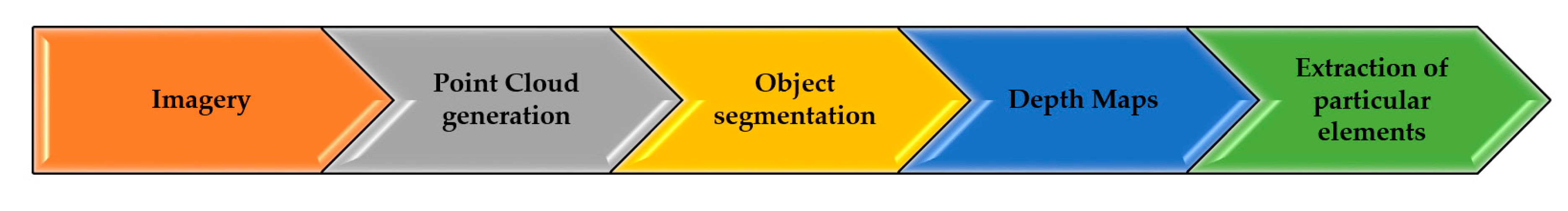
2.3. Application of Random Sampling Consensus (RANSAC) Segmentation Algorithm

Once the accuracy of the models was established, the next step was to focus on segmenting the 3D models. The first strategy analyzed to do this was the random sampling consensus (RANSAC) segmentation algorithm. The RANSAC was utilized to extract shapes from a derived model. This was done by assigning sets of points that can define a particular geometric feature type and then extracting shapes that fit this feature type based on the number of points in the category [44].

The algorithm functions by taking a given point-cloud P = {p₁, ..., p_N} with associated normals {n₁, ..., n_N} giving an output of a set of primitive shapes Ψ = {Ψ₁, ..., Ψ_n} with corresponding disjoint sets of points P_Ψ1 ⊂ P, ..., P_Ψn ⊂ P and a set of remaining points R = P\{P_Ψ1, ..., P_Ψn}. For every iteration of the algorithm, the primitive with the highest score is sought after. The algorithm iteration will conclude as soon as the defined minimal shape size is achieved for the point cloud. The definition of this minimal shape size can be controlled and for this study, this value was based on the size of the point cloud being analyzed. This process can be visualized in the pseudocode for Algorithm 1 shown below as created by [44]:

Algorithm 1 Extracting shapes in point Cloud Ρ

Ψ ← Ø {extracted shapes} C ← Ø {shape candidates} repeat  C ← C ∪ new Candidates()  m ← best Candidate (C)  if P(|m|, |C|> pt then    P ← P \Pm {remove points}    Ψ ← Ψ ∪ m    C ← C \ Cm {remove invalid candidates}  end if until P(τ, |C|> pt return Ψ

The implementation of this algorithm was done within CloudCompare, utilizing the H-RANSAC plugin. This process is able to isolate several different shapes from the model in question including planes, spheres, cylinders, cones, and tori. For the purpose of this study, the focus was on the planes so as to generate a profile for the pavement to deduce the distressed areas. The purpose, therefore, would be to identify an appropriate plane to be used as a baseline for creating a road profile and to generate depth maps of the section which are able to be metrically referenced. Once the maps are created the particular points of interest on the model can be established and isolated.

2.4. Application of ‘Fit’ Algorithm

As an alternative to the RANSAC segmentation pipeline, another possible way of segmenting the pavement was utilizing the fit algorithm within the CloudCompare suite. The fit tool creates a plane based on the points within the point cloud. It, therefore, considers the entire point cloud under analysis. To do this the process utilizes a standard least square fitting methodology of the points within the point cloud. This is based directly on the eigenvalues and vectors of the covariance matrix of the cloud so it can be considered as an efficient process.

Once this tool is applied, the distance of this plane from the point cloud can again be utilized to create a profile of the measured differences which will generate a depth map to understand the conditions of the pavement section. The depth maps generated from this simple methodology were compared to those from the RANSAC.

3. Results and Discussion

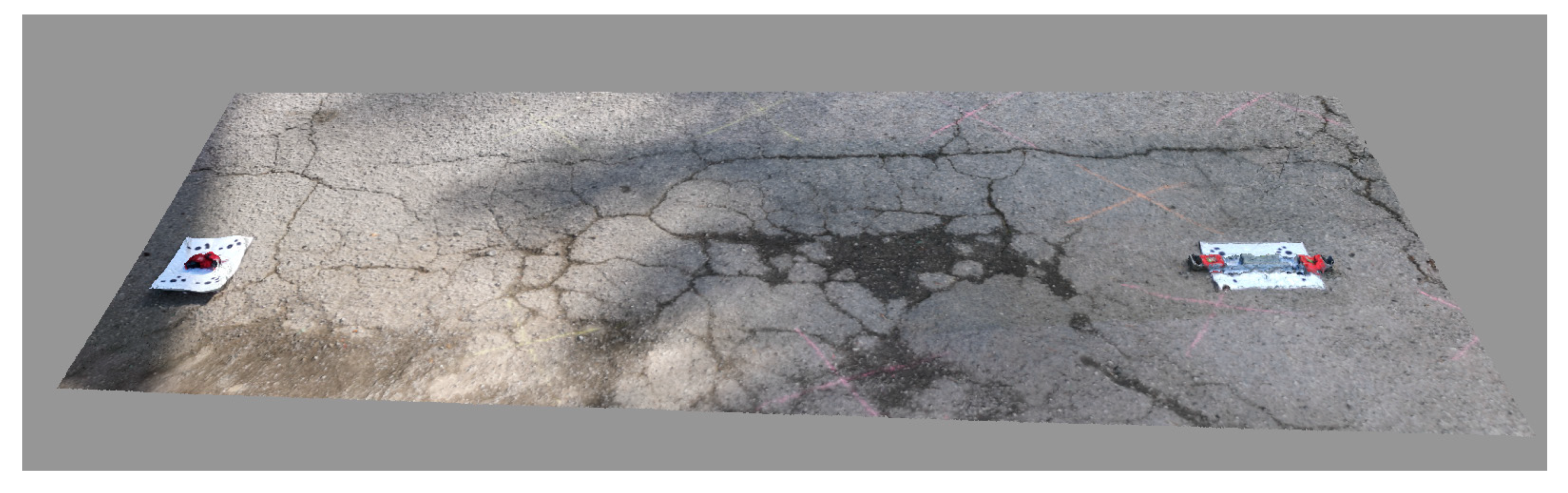
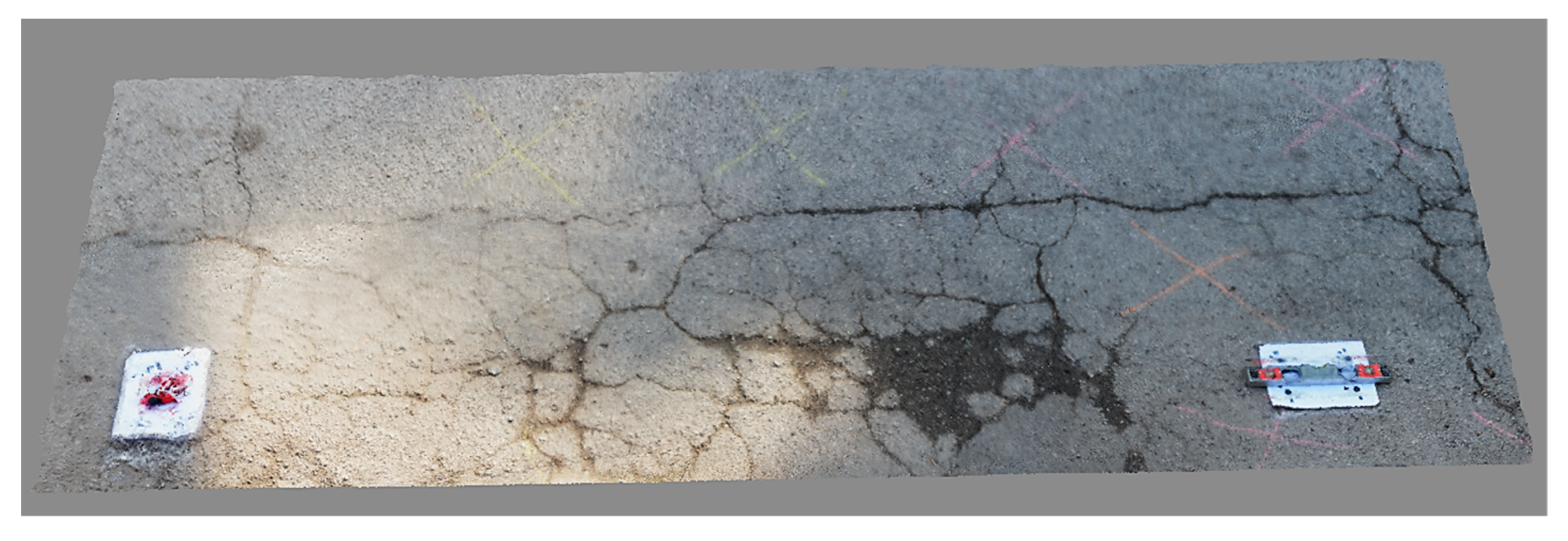
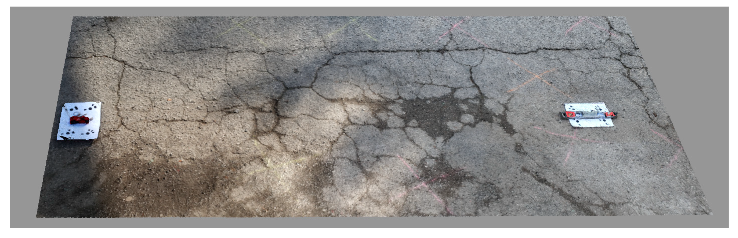
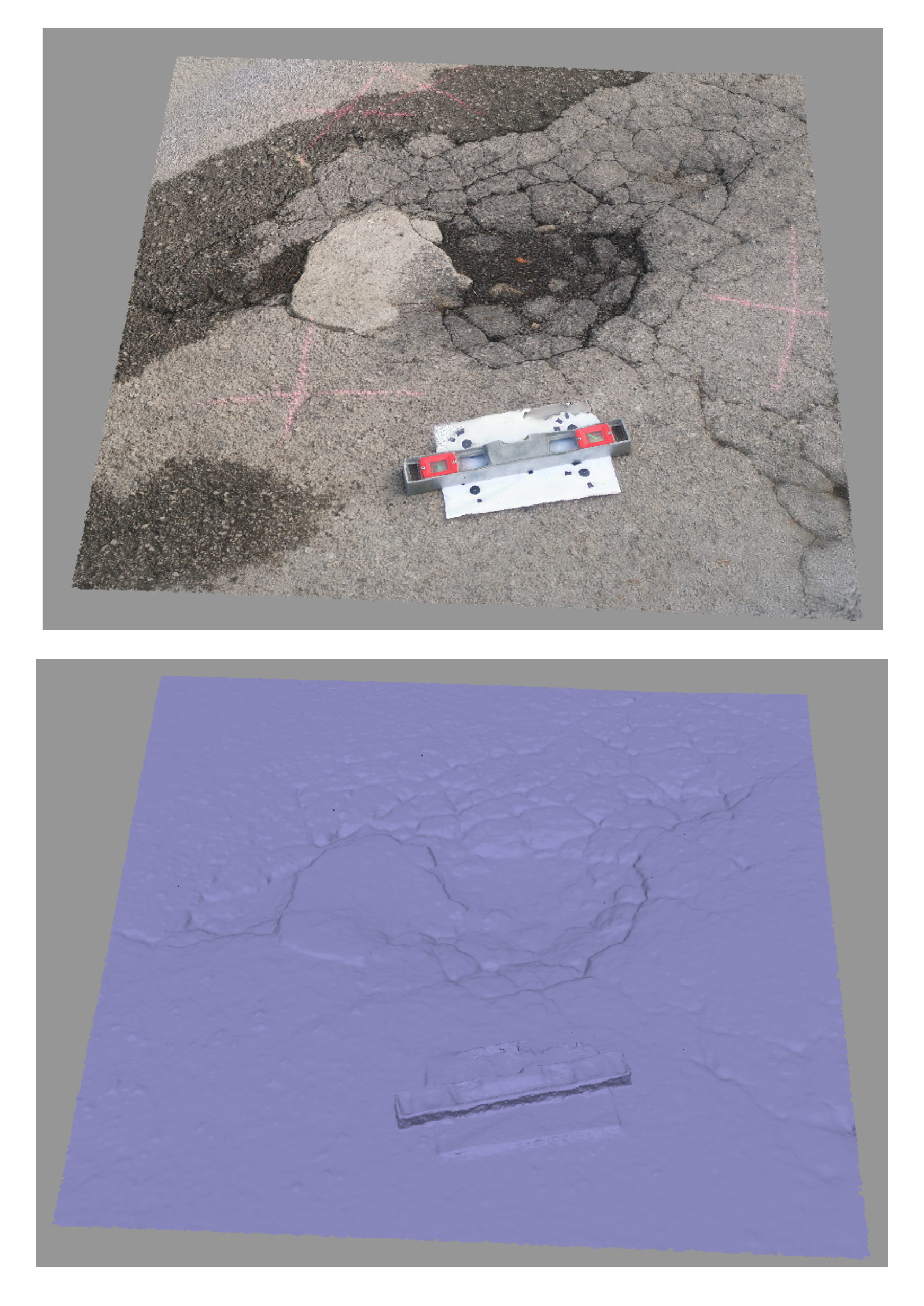
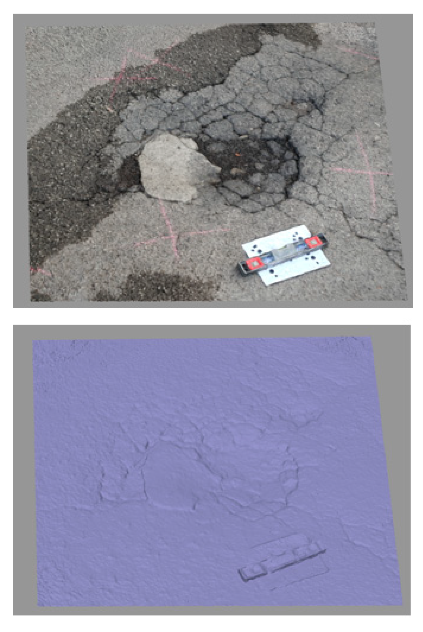
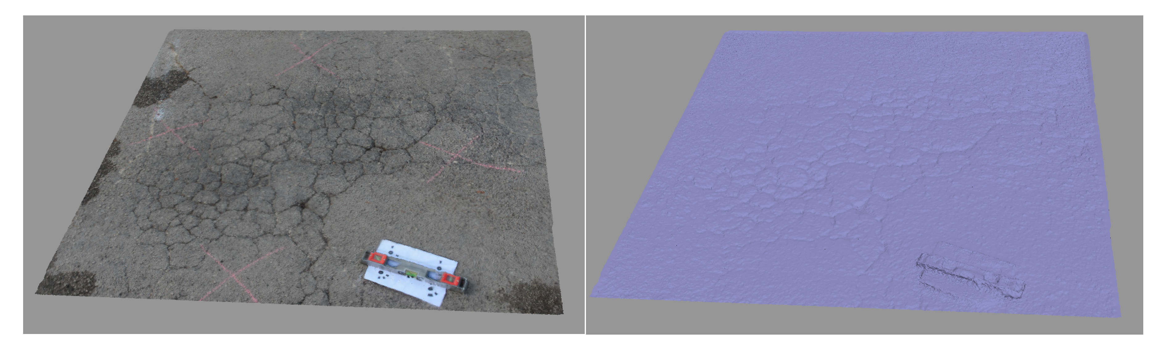
3.1. D Pavement Distress Models

3.1.1. Pavement Section 1

For each section under analysis, the results of the mobile imagery were compared to those from the camera. In

Table 2. Survey specifications for Distress 1.

Device	Nikon D5200	Huawei P20 Pro	Samsung Galaxy S9
Distance from the pavement [mm]	~1500	~1500	~1500
Number of photos taken [-]	46	55	57
Ground sample distance (GSD) [mm/pixel]	0.241	0.547	0.505
Mesh faces created in SfM software [-]	4,800,185	2,155,780	2,900,791

, the specifications and results of the models for each device are shown for the survey of the first section. It can be observed that the GSD for the camera-based model was the lowest and this is expected given the higher resolution capable from this device. This is a direct result of the focal length of a professional camera being substantially higher than a mobile device. This also is the reason why the professional camera was used as a comparison model. However, the achieved GSD values for both devices were ~0.5 mm which is sufficient given the requirements for the detection of pavement distresses as previously examined in Section 2.1. The other parameter in Table 2 is the number of mesh faces of each model. This is a parameter that indicates the number of details on the models. However, it is hard to decipher based on the number and a visual inspection of the model is a better approach to analyze the models’ details. Images of each replicated model for the section are given in Figure 7, Figure 8 and Figure 9. Based on these figures, the details of the cracked section are shown. There were some differences in the colors of the models and this can be related to the internal parameters of the camera devices. The visual inspection, however, has no bearing on the accuracy for distress detection and a metric evaluation is needed to understand accuracies.

3.1.2. Pavement Section 2

For the second pavement section, the resulting specifications from the models produced are given in

Table 3. Survey specifications for Distress 2.

Device	Nikon D5200	Huawei P20 Pro	Samsung Galaxy S9
Distance from the pavement [mm]	~1500	~1500	~1500
Number of photos taken [-]	38	58	62
Ground sample distance (GSD) [mm/pixel]	0.322	0.567	0.485
Mesh faces created in SfM software [-]	4,615,825	1,912,697	2,022,877

. Similar to the first section, it is observed that the GSD was smaller for the camera derived model but the values for the models produced by the mobile phones were once again sufficient for detecting the pavement distresses.

The models produced by the mobile imagery for this section are shown in Figure 10 and Figure 11. Also shown are images of the dense clouds produced by mobile imagery. These dense clouds allow for an inspection of the roughness and texture of the pavement and also allows the user to see clearly the distressed sections of the pavement. They are visualized here as this section also has a depressed area within the pavement and with the dense cloud, this is easier to visualize and detect.

3.1.3. Pavement Section 3

For the third section, the resulting specifications from the models produced are given in

Table 4. Survey specifications for distress 3.

Device	Nikon D5200	Huawei P20 Pro	Samsung Galaxy S9
Distance from the pavement [mm]	~1500	~1500	~1500
Number of photos taken [-]	42	42	58
Ground sample distance (GSD) [mm/pixel]	0.318	0.596	0.458
Mesh faces created in SfM software [-]	3,151,044	1,486,123	1,900,926

. Similar to the previous sections, the GSD was smaller for the camera derived model but the values for the models produced by the mobile phones were once again sufficient for detecting the pavement distresses. The models produced by the mobile imagery for this section are shown in Figure 12 and Figure 13. Also displayed are images of the dense clouds produced by mobile imagery. Within the dense clouds, one can again observe the cracked section and the contours created by these cracks. This visualization can enable easier segmentation of the section for analysis of the cracks for metric severity analysis.

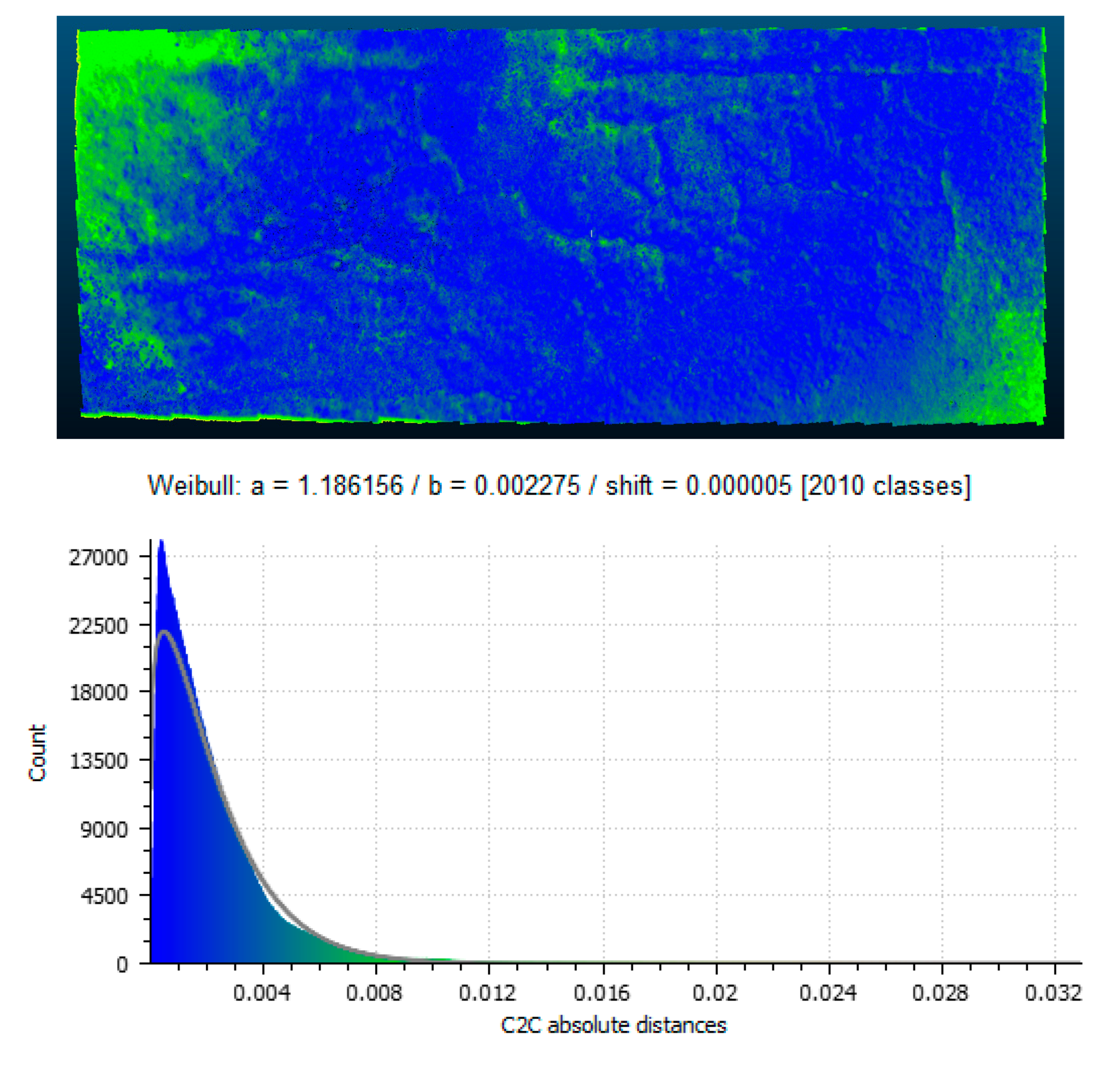
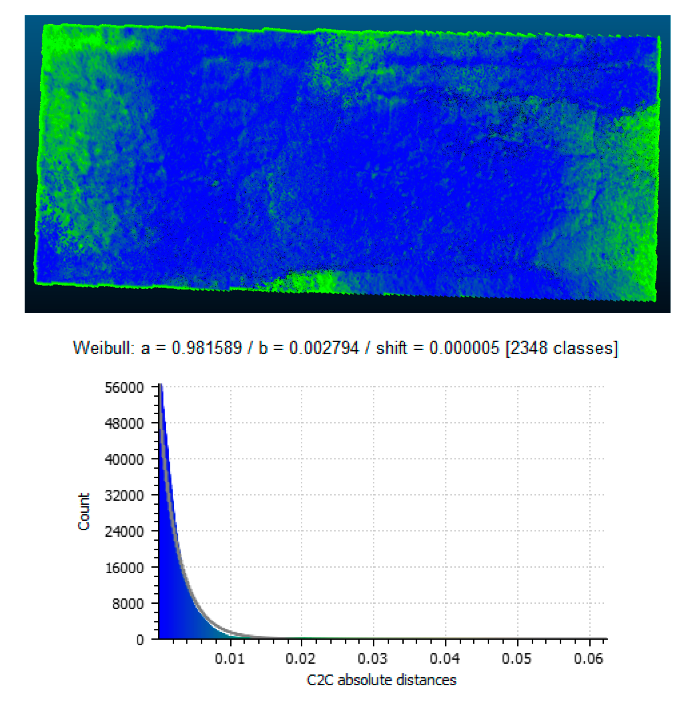
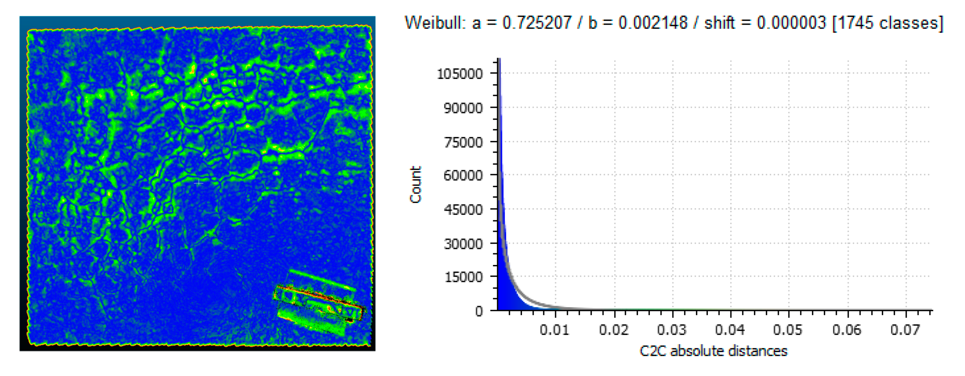
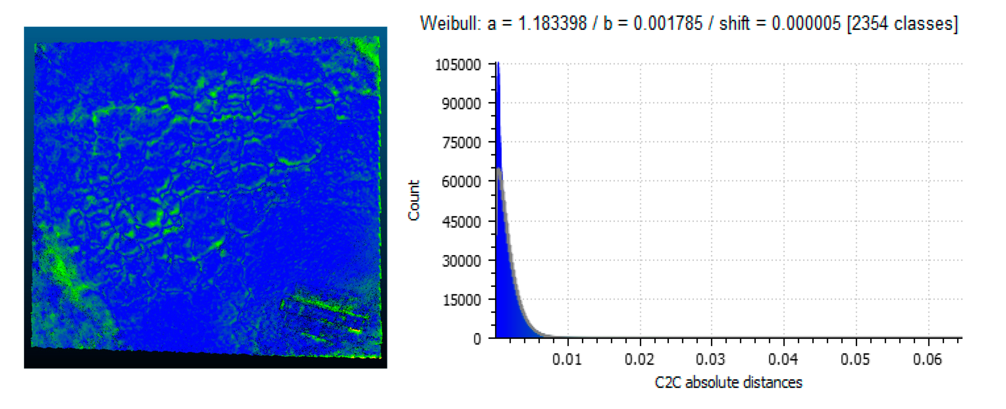
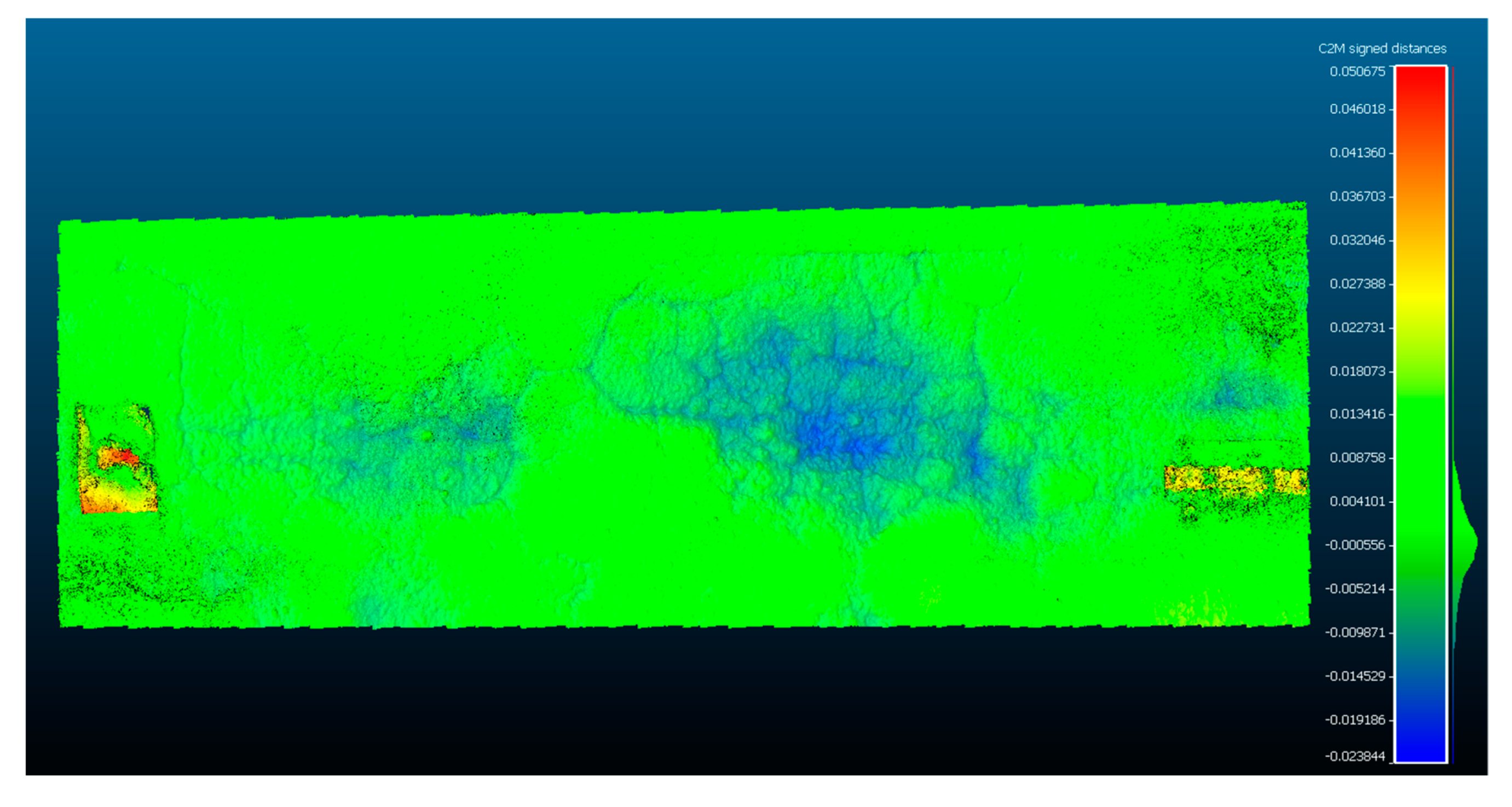
3.2. Accuracy of 3D Models Generated by Imagery from Mobile Phones

After the models were replicated using the SfM pipeline, they were then imported into CloudCompare, which is a software designed to analyze 3D models and point clouds. In the software, the models derived by the mobile imagery were aligned with the models derived by the camera. This alignment was done utilizing common points between the models so as to create a scenario where the two models are effectively overlapped at the correct points. Once the alignment was complete the distances between them were measured using a metric called C2C (Cloud to Cloud) absolute distance. This measurement produces a visualization of the measured differences across the model’s surface. This visualization is also color coded with a color range of blue to red with blue highlighting smaller differences and red highlighting larger ones. From these differences, a histogram can be plotted illustrating the differences. Using the differences illustrated, the Weibull distribution was also applied to determine the Weibull parameters of shape and scale in order to have a statistical metric understanding of the differences.

3.2.1. Pavement Section 1

For the first section, the visualized differences along with the plotted distribution and Weibull plot are shown in Figure 14 and Figure 15. The two important resulting parameters from this distribution are the Weibull shape and scale parameters and the values for these are given in

Table 5. Weibull parameters observed from each model comparison for Distressed Section 1.

	Weibull Parameters
Phone	Shape (a)	Scale (b)
Huawei P20 Pro	1.186156	0.002275
Samsung Galaxy s9	0.981589	0.002794

where the scale parameter would be measured in metres and the shape parameter has no dimension. The scale value typically specifies that 63.2 percentile of the distribution will fail before reaching this point [45]. Given the values in the table, this signifies that for all of the models this value was less than 0.003 m (3 mm). Furthermore, the value of the shape parameter was also close to 1 which signifies that within the distribution it is more likely that the majority of the values will occur early in the plot. Therefore, it can be inferred that for a random point on the model, it is likely that it would have a small measured difference as the small differences are the values that occur early in the distribution plot. This helps to validate the hypothesis of using low-cost mobile imagery for this section. The visualizations provided also depicted the locations on the pavement where the most change is present. This was generally along the inside of the cracks as can be demonstrated in Figure 14 and Figure 15. Future work will consider the range of values of the two Weibull parameters for a myriad of different distresses and phone types to try and establish more particular correlations and trends of these parameters based on the distresses.

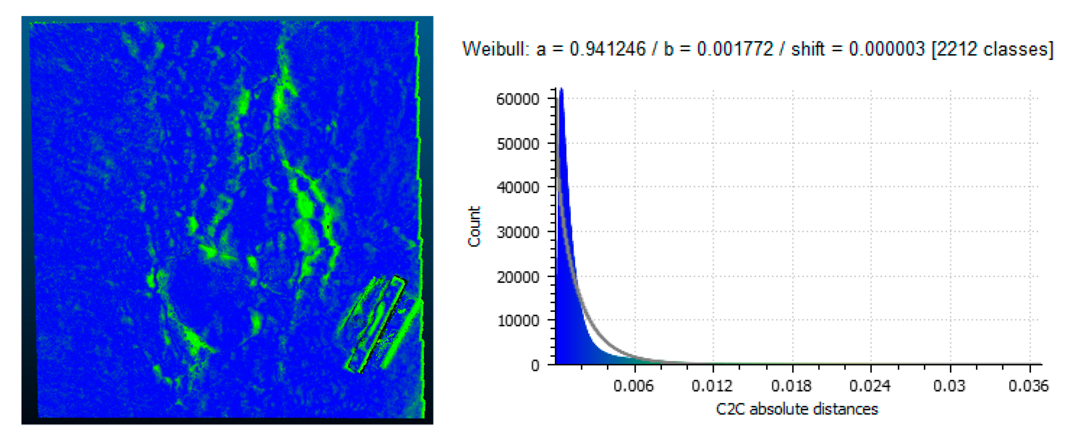
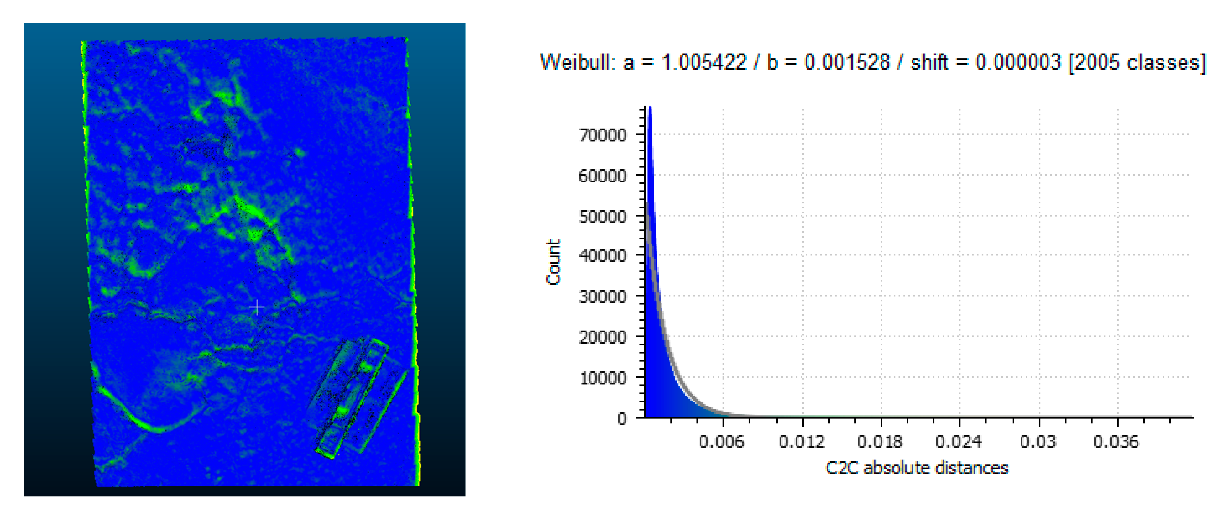
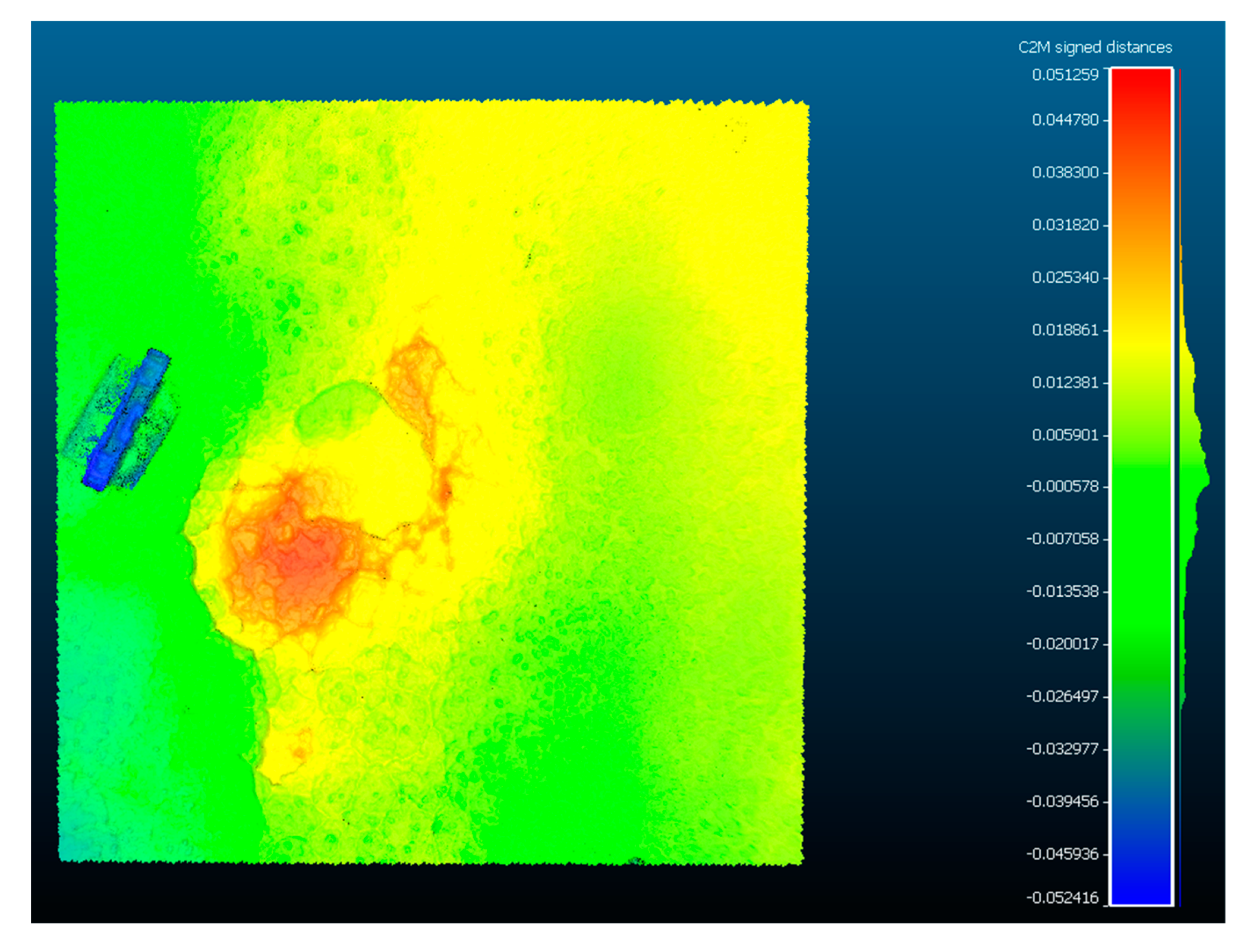
3.2.2. Pavement Section 2

For the second section, the visualized differences along with the plotted distribution and Weibull plot are shown in Figure 16 and Figure 17. The Weibull shape and scale parameters are also given in

Table 6. Weibull parameters observed from each model comparison for distressed section 2.

	Weibull Parameters
Phone	Shape (a)	Scale (b)
Huawei P20 Pro	0.941246	0.001772
Samsung Galaxy s9	1.005422	0.001528

. For this section, the values for the scale were again less than 0.003 m (3 mm). The value of the shape parameter was again close to 1 which once more signifies that within the distribution it is more likely that the majority of the values will occur early in the plot. This helps to reinforce the validity of the methodology for a different section, this one with depressions and cracking. The visualizations for these two comparisons showed that the most change occurred along the crack but also in the interior of the depression present in the section.

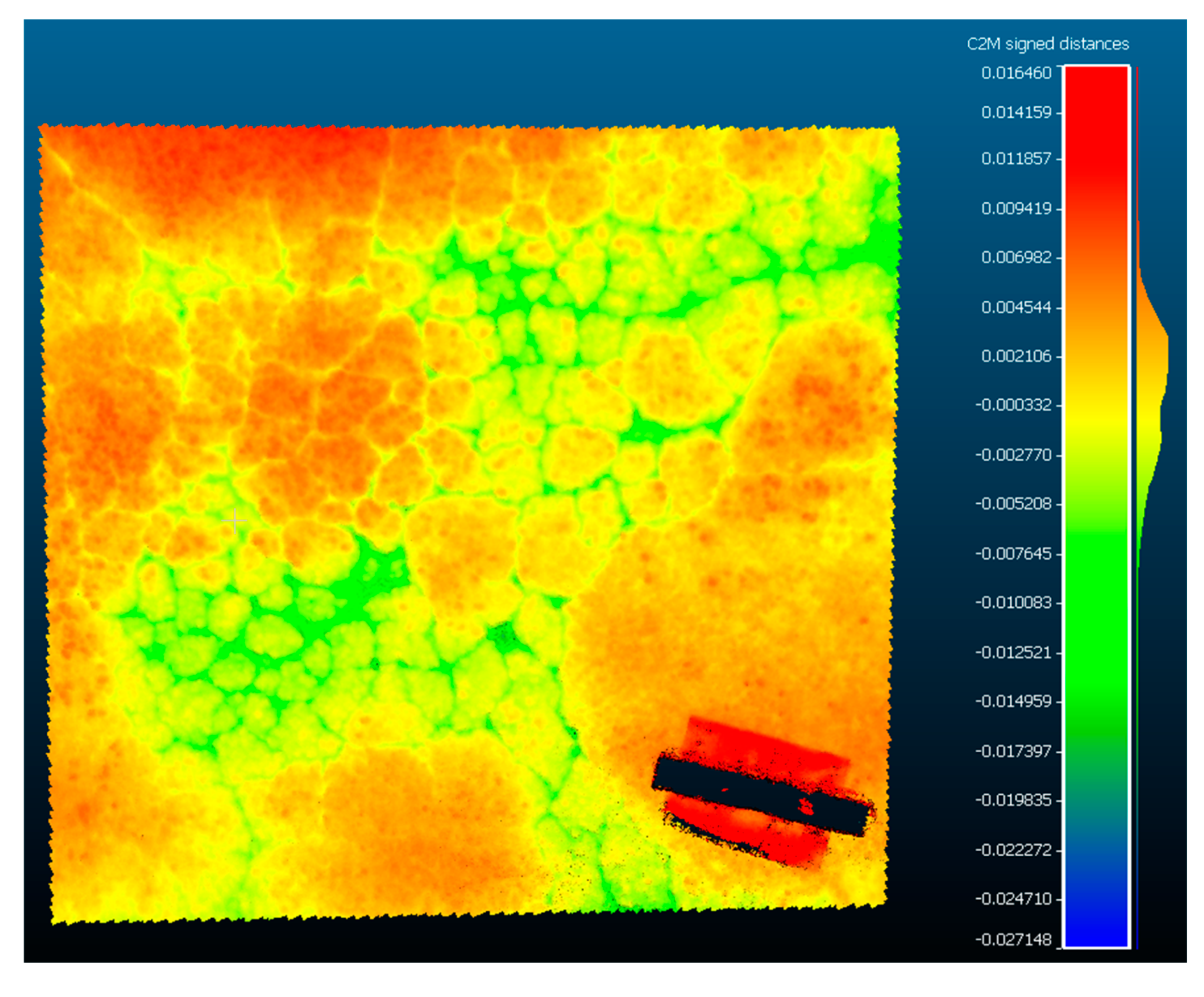
3.2.3. Pavement Section 3

For the third section, the visualized differences along with the plotted distribution and Weibull plot are shown in Figure 18 and Figure 19. The Weibull shape and scale parameters are also given in

Table 7. Weibull parameters observed from each model comparison for distressed Section 3.

	Weibull Parameters
Phone	Shape (a)	Scale (b)
Huawei P20 Pro	0.725207	0.002148
Samsung Galaxy s9	1.183398	0.001785

. For this section the values for the scale were again less than 0.003 m (3 mm). Additionally as was the case with the two previous sections, the shape parameter was again close to 1 which once more signifies that within the distribution it is more likely that the majority of the values will occur early in the plot. Once more this reinforces the validity of the methodology for a different section, this one with area-wide cracking that are block and alligator-like. The visualizations for these two comparisons showed that the most change occurred along the interiors of the blocks of the crack

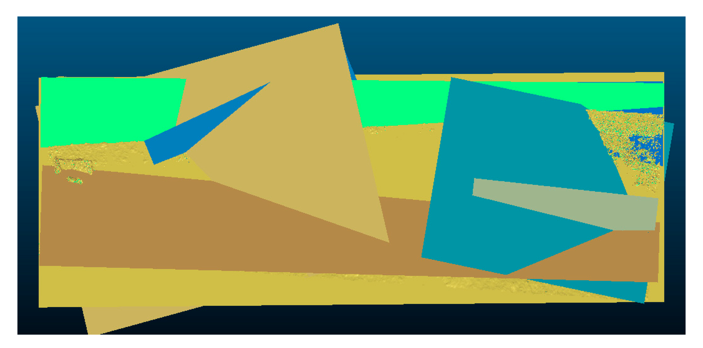
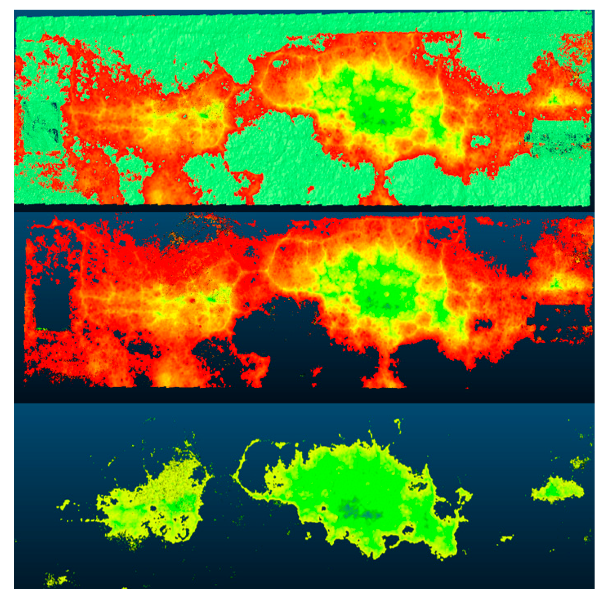
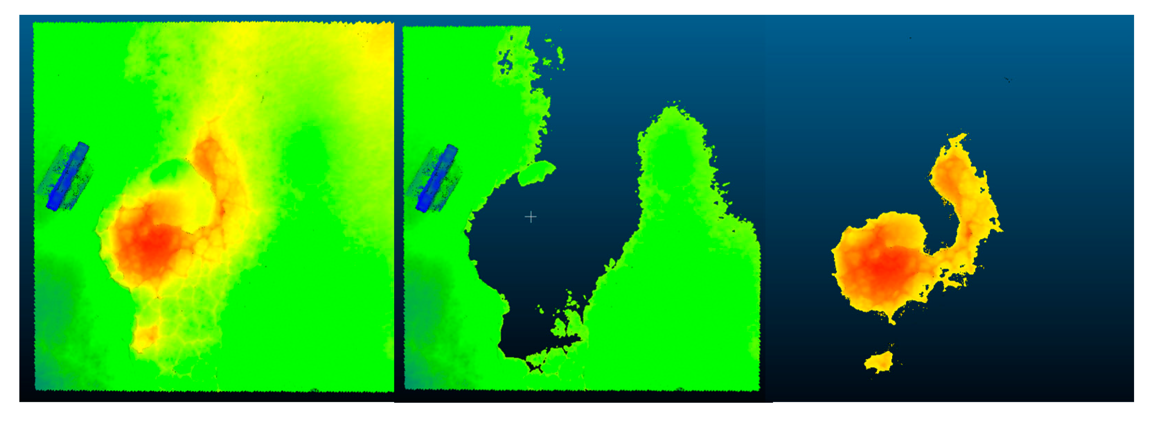
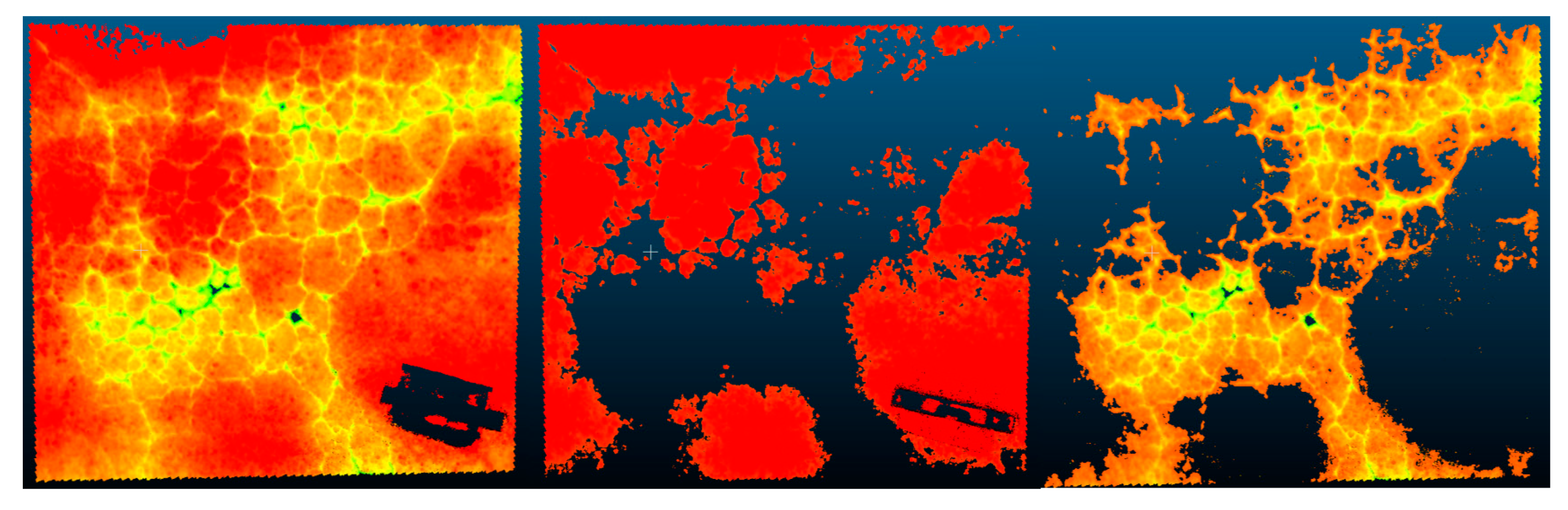
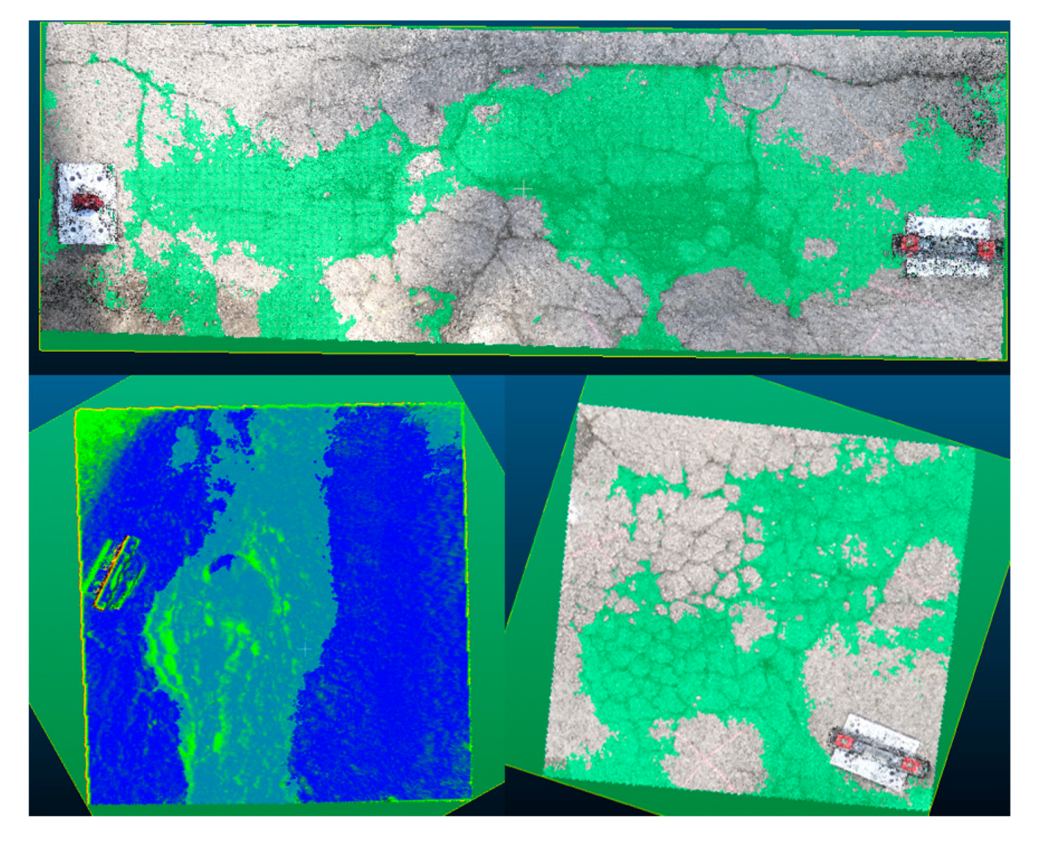
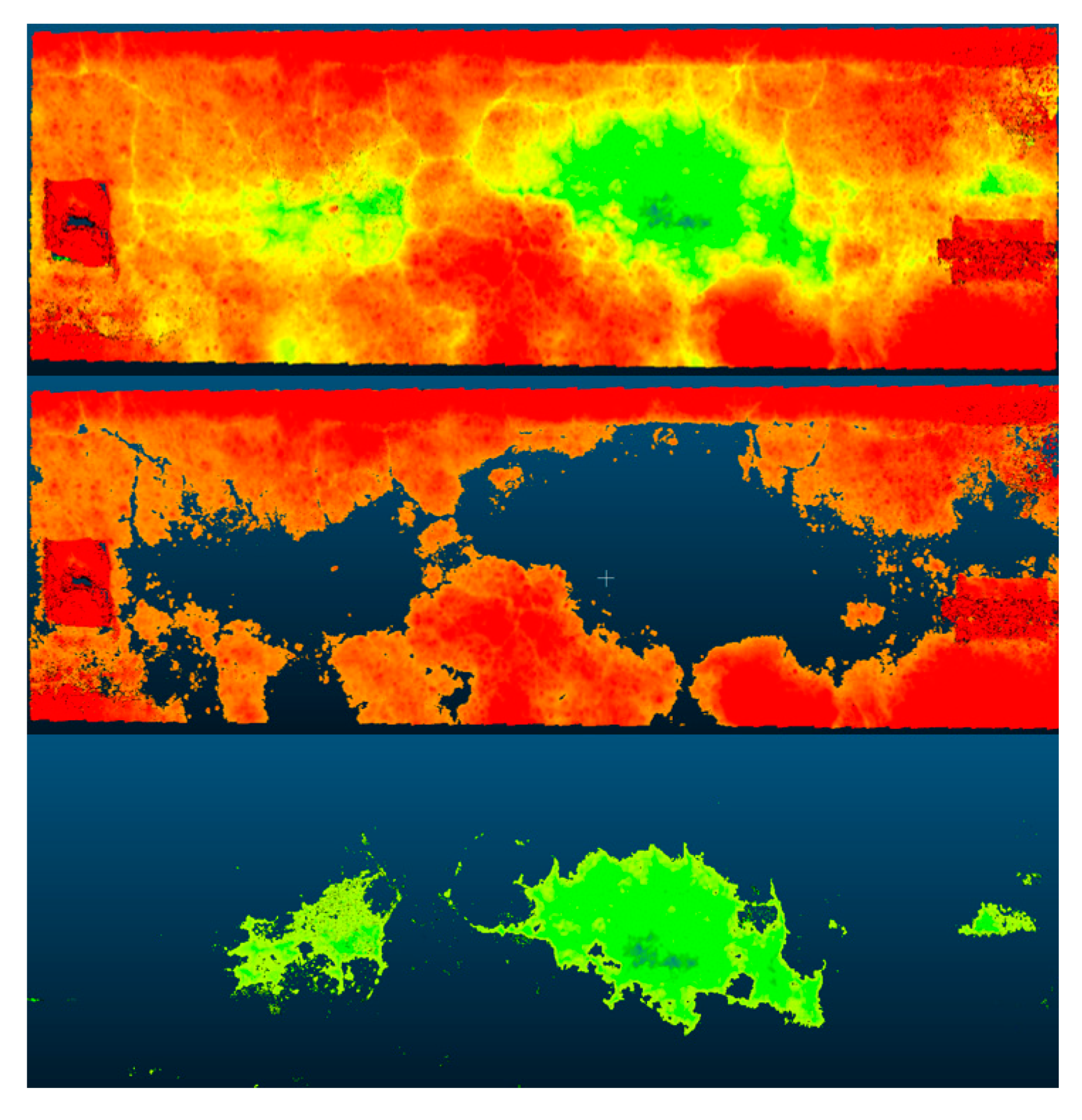
3.3. Application of RANSAC Segmentation

Once the accuracy of the models was demonstrated as shown in the previous section, the next step was the application of the segmentation strategies to try and isolate the distresses occurring on each pavement section in the case study. The first considered strategy was the use of the RANSAC algorithm to extract shapes from the point clouds.

The first step for this implementation was assigning a value of the minimum support points per primitive. For each of the models being analyzed the total number of points was between 1.4 to 4.5 million points. Additionally, each model assumed a physical distance of about 2 to 4 m² on ground. Given these factors, a value of 50,000 was assigned as this would split the object into no more than 90 segments and given the fact that only one plane was required as a reference case this number would limit the algorithm from producing planes cutting through the model at different mismatched angles. To ensure this value was correct the algorithm was applied for smaller values of 500, 5000, 10,000 and each of these scenarios inappropriate planes were generated as shown in Figure 20. This process was tried for each model and it was shown that with 50,000 points the result would yield an appropriate reference plane as shown through an example of one of the applications in Figure 21. On this, the plane appropriately cuts through the model to create a valid reference plane.

Once this plane was adequately assigned a distance computation between the plane mesh and the point cloud was done utilizing the C2M distance computation in CloudCompare to produce a depth map for each distress. The C2M distances represent the depths and filtering this can result in the segmentation of the model. This is illustrated in Figure 22, Figure 23 and Figure 24.

These depth maps now allow filtering to be done by depth and section and allow the model to be segmented for the sections to be analyzed. This is easily done by controlling the range of the depth map and this is illustrated in Figure 25, Figure 26 and Figure 27. From the current segmentation result, the process can detect typical distresses where there is a change in surface deviation of the pavement. As the major groups of pavements distresses are cracking distresses and visco-plastic deformations (which both feature this type of deviation), this process and segmentation can account for most distresses. Visco-plastic deformations include bumps, sagging, rutting, corrugations, depressions, potholes, swelling, lane and shoulder drop off, shoving, and stripping. In Figure 25, Figure 26 and Figure 27, the depth maps for the pavement sections are shown at three different levels of segmentation. In the first image, the entire section is visualized with the hotspots of the distressed sections highlighted. Given that in this depth map one can see the particular points of interest, the depth map was then further segmented to remove the parts of the pavement without distress by using a smaller range on the depth map values. The final image of the three further adjusts the range of the depth map to then only illustrate the distressed section with the deepest distress. In Figure 25, the third image highlights the section suffering from not only cracking but also a significant depression. The same process was carried out for each section and the visualizations are shown in Figure 26 and Figure 27 also follow the same methodology to allow visualization of the exact points of distress and to isolate these sections. In Figure 26, the exact section suffering from a pothole is isolated and in Figure 27, the exact section suffering from excessive cracking is isolated. The exact metric evaluation of the distress is not shown within the study as the metric evaluation of 3D models derived from SfM processes has been previously validated using laser equipment to verify the metric accuracy of the models to determine the closeness of the results from those measured within the field [20,27]. The semantic color choice of the depth map is up to the user for the visualizations, in terms of which colors signify positive or negative deviations. Once this segmentation is done, metric assessments of the segmented portion can be found such as the area and volume of the segmented region which can either be the section that is distressed or the section that is not. By doing this, a ratio of the distressed section to non-distressed section can be established and inserted into the asset database for the road authorities, which is critical for establishing appropriate pavement management strategies. These critiques are possible as all of the models are scaled and the previous sections have established the metric accuracy of these scaled models. The dimensional analysis of the sections was not carried out as the determination of the methodology to arrive at a position at which this type of analysis is possible was more important to the discussion of the study and the research. Additionally features such as the depressed section and the crack section be filtered by simply changing the range of the depth map as shown in the images. From this segmentation, a differentiation of the types of distresses occurring can be made as well as the particular features of the distress can be more easily identified as the depth maps shown in Figure 25, Figure 26 and Figure 27 establish isolation of sections that have related features. At this point, the user would be able to identify the particular distress type. This will provide a road agency with exact measurements of the distress which can be utilized for severity assessment and to trigger times for maintenance and rehabilitation interventions.

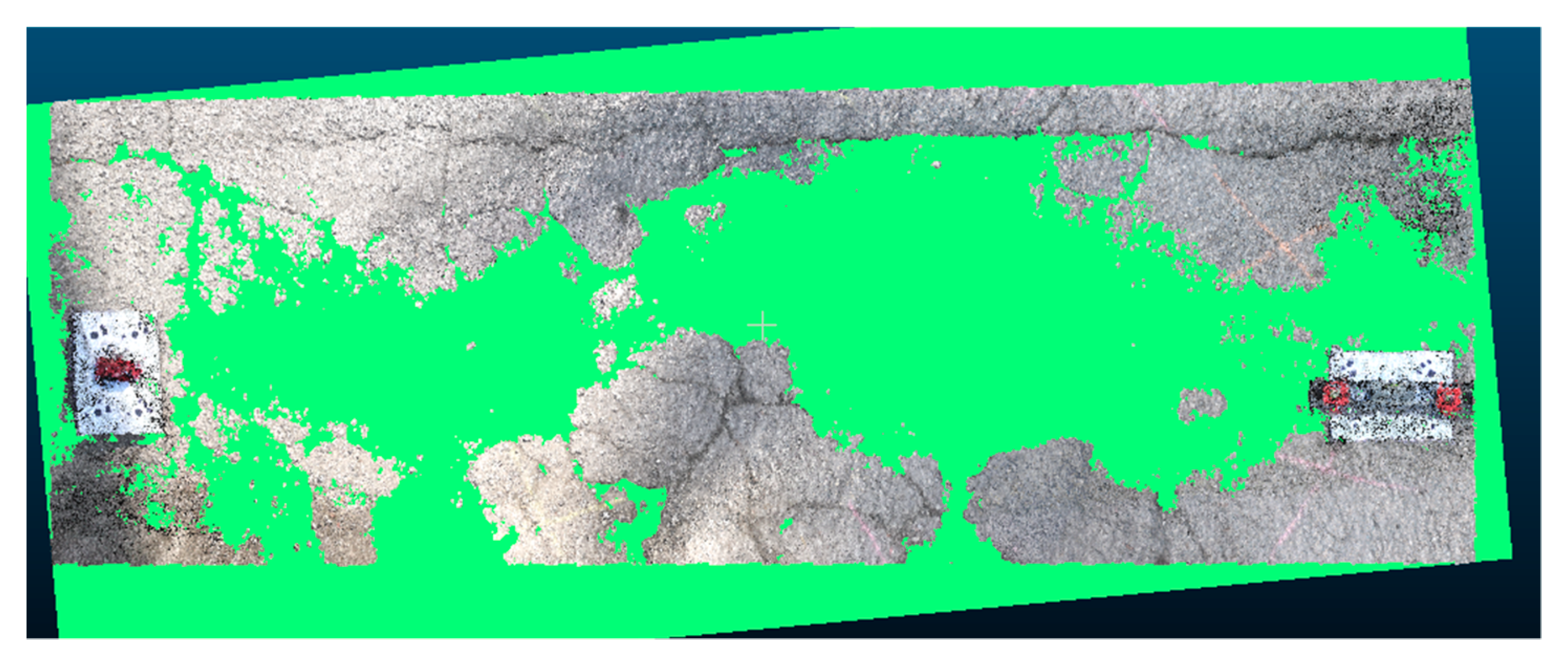
3.4. Application of Fit Segmentation

For the application of the fit algorithm, a similar process was followed to that of the RANSAC wherein a plane was generated considering the collection of points within the point cloud. This application can be considered as a simpler method given the fact that it relies on a standard least square fitting methodology. The application of the fit tool was carried out on each model and this is demonstrated in Figure 28.

Following this plane application, the depth maps were generated on each model similar to the application of the RANSAC. This was done for the same purpose as previously stated to allow for segmenting particular sections of the pavement sections. This is illustrated in Figure 29, Figure 30 and Figure 31.

Similar to the segmented images of the sections by the RANSAC algorithm, these images represent three levels of segmentation for each distress and highlight the possibility of isolating particular points of interest by altering the range of the displayed depth map. The segmented images depict particular points of interest. Each isolation can be measured and the metric value recorded for the purpose of collecting asset information and storing in within the database of the road authority or agency.

Figure 29 demonstrate the capacity of using the fit plane. In each segmentation particular sections can be isolated. The sections where there is cracking can be isolated or the sections where there is a depression. The same can be done for the sections which are in suitable conditions. The results are similar to those obtained with the RANSAC. A metric difference between the segmented models was not however done as more examples are needed for this to be done. This will be explored in future works.

The essential conclusion from both segmentation applications is that the process has the capacity to produce the resulting isolated sections of the mobile imagery-based 3D models. These isolated segments can yield critical metric information as they are scaled and the accuracy of the derived models was shown to be sufficient for the purpose of detecting pavement distresses. The extraction of the metric information of the distresses and the segmented sections are not carried out within this study but the previous analysis of 3D models originating from an SfM pipeline have already demonstrated this possibility [20]. The methodology of segmenting the imagery and thus exploiting it for further analysis is the important outcome of this aspect of the study. Additionally, this process was done with user-friendly algorithms that can be practically repeated and do not require substantial processing power or exhaustive timelines utilized by other pipelines.

4. Conclusions

This work provided within this paper had two particular purposes: demonstrate the accuracies of utilizing imagery from mobile phones for creating 3D models of pavement distresses and secondly to consider practical and efficient means of segmenting these models to isolate pavement distresses. The purpose, therefore, was to establish a workable pipeline with mobile phone devices. To carry out these tasks, surveys were carried out on distressed pavement sections within the city of Palermo, Italy where there are a substantial number of distressed roads. Three sections were considered which had commonly found pavement distresses. Each section was surveyed with two common mobile phones and a professional camera was used as a control in the experiment.

Using statistical analysis and comparison, it was found that the SfM techniques discussed can be utilized with the mobile devices used in the study with accurate models being generated that can sufficiently detect the precedence of pavement distresses within the sections. The statistical analysis was done utilizing the Weibull distribution evaluation with comparisons being made from models generated from the mobile devices to the models generated from a professional camera. The Weibull parameters yielded in the evaluation detailed that the majority of the deviations between the models are of very small values, in the range of less than 3 mm. This value allows for authentication of the pipeline with the mobile devices based on the typical measurement of common pavement distresses. This represents a novel approach to the problem and based on advances in the phone industry future results will be even more promising. Furthermore, it should be noted that the mobile phones used in the study are not the latest flagship models from their respective companies and that there are newer models currently on the market which have better cameras and therefore, would likely yield models with greater resolutions. This demonstrates the capacity and sustainability of the pipeline moving forward. Further work can include further assessments of other mobile phones and more types of pavement distresses. Additionally, it was must be mentioned that the use of mobile devices poses advantages to other methods of obtaining imagery such as drones which have legal restrictions in many countries. For future work imagery from Google Earth’s platform can also be combined with imagery from the mobile phones to have a bigger model developed encompassing a full network and not just a particular section. This is possible as the imagery from Google Earth has been integrated with on-ground 2D imagery for applications in other fields [46].

After the considerations of the accuracy of the 3D models, the study carried out a brief analysis of the segmentation of the 3D imagery. Planes were constructed on the models utilizing different algorithms for the purpose of creating depth maps and these depth maps were then filtered based on the location and presence of distresses within the pavement section. By filtering the models, the model was segmented based on similarly observed features which can allow for a differentiation of the different pavement distress categories. Additionally, the segmentation of the particular points of interest allows the user to obtain a ratio of the distressed area to the non-distressed area on the pavement section which is a valuable attribute for the road authority’s database. This demonstrated the capacity of the segmentation pipeline to pinpoint occurring distresses and obtain metric information on them. Further work needs to be done on larger sections and more types of pavement distresses to establish a clear segmentation pipeline for these types of images. Nevertheless, the segmentation strategies used were demonstrated to be potent enough to isolate the pavement distresses and this establishes a path forward towards the full low-cost automation of road condition data acquisition and analysis for a pavement management.

References

1. Vandam, T.J.; Harvey, J.T.; Muench, S.T.; Smith, K.D.; Snyder, M.B.; Al-Qadi, I.L.; Ozer, H.; Meijer, J.; Ram, P.V.; Roesier, J.R.; et al. Towards Sustainable Pavement Systems: A Reference Document FHWA-HIF-15-002; United States Federal Highway Administration: Washington, DC, USA, 2015. [Google Scholar]
2. International Road Federation (IRF). IRF World Road Statistics 2018 (Data 2011–2016); International Road Federation (IRF): Brussels, Belgium, 2018. [Google Scholar]
3. Mbara, T.C.; Nyarirangwe, M.; Mukwashi, T. Challenges of raising road maintenance funds in developing countries: An analysis of road tolling in Zimbabwe. J. Transp. Supply Chain Manag. 2012, 4, 151–175. [Google Scholar] [CrossRef] [Green Version]
4. Peterson, D. National Cooperative Highway Research Program Synthesis of Highway Practice Pavement Management Practices; Transportation Research Board: Washington, DC, USA, 1987; No. 135; ISBN 0309044197. [Google Scholar]
5. Kulkarni, R.B.; Miller, R.W. Pavement Management Systems: Past, Present, and Future. Transp. Res. Rec. J. Transp. Res. Board 2003, 1853, 65–71. [Google Scholar] [CrossRef]
6. Schnebele, E.; Tanyu, B.F.; Cervone, G.; Waters, N. Review of remote sensing methodologies for pavement management and assessment. Eur. Transp. Res. Rev. 2015, 7, 7. [Google Scholar] [CrossRef] [Green Version]
7. Radopoulou, S.C.; Brilakis, I. Improving Road Asset Condition Monitoring. Transp. Res. Procedia 2016, 14, 3004–3012. [Google Scholar] [CrossRef] [Green Version]
8. Coenen, T.B.J.; Golroo, A. A review on automated pavement distress detection methods. Cogent Eng. 2017, 4, 1374822. [Google Scholar] [CrossRef]
9. Ragnoli, A.; De Blasiis, M.; Di Benedetto, A. Pavement Distress Detection Methods: A Review. Infrastructures 2018, 3, 58. [Google Scholar] [CrossRef] [Green Version]
10. Laurent, J.; Hébert, J.F.; Lefebvre, D.; Savard, Y. Using 3D Laser Profiling Sensors for the Automated Measurement of Road Surface Conditions. In 7th RILEM International Conference on Cracking in Pavements; Scarpas, A., Kringos, N., Al-Qadi, I.A.L., Eds.; Springer: Dordrecht, The Netherlands, 2012; pp. 157–167. [Google Scholar]
11. Landa, J.; Prochazka, D. Automatic Road Inventory Using LiDAR. Procedia Econ. Financ. 2014, 12, 363–370. [Google Scholar] [CrossRef] [Green Version]
12. Sairam, N.; Nagarajan, S.; Ornitz, S. Development of Mobile Mapping System for 3D Road Asset Inventory. Sensors 2016, 16, 367. [Google Scholar] [CrossRef] [Green Version]
13. Arhin, S.A.; Williams, L.N.; Ribbiso, A.; Anderson, M.F. Predicting Pavement Condition Index Using International Roughness Index in a Dense Urban Area. J. Civ. Eng. Res. 2015, 5, 10–17. [Google Scholar]
14. Wix, R.; Leschinski, R. Cracking—A Tale of Four Systems. In Proceedings of the 25th Australian Road Research Board Conference, Perth, Australia, 23–26 September 2012; pp. 1–20. [Google Scholar]
15. Oliveira, H.; Correia, P.L. Automatic road crack detection and characterization. IEEE Trans. Intell. Transp. Syst. 2013, 14, 155–168. [Google Scholar] [CrossRef]
16. Wang, K.C.P.; Gong, W. Automated pavement distress survey: A review and a new direction. In Proceedings of the Pavement Evaluation Conference, Roanoke, VA, USA, 21–25 October 2002; pp. 21–25. [Google Scholar]
17. Puan, O.C.; Mustaffar, M.; Ling, T.-C. Automated Pavement Imaging Program (APIP) for Pavement Cracks Classification and Quantification. Malays. J. Civ. Eng. 2007, 19, 1–16. [Google Scholar]
18. Chambon, S.; Moliard, J.M. Automatic road pavement assessment with image processing: Review and Comparison. Int. J. Geophys. 2011, 2011, 989354. [Google Scholar] [CrossRef] [Green Version]
19. Zakeri, H.; Nejad, F.M.; Fahimifar, A. Image Based Techniques for Crack Detection, Classification and Quantification in Asphalt Pavement: A Review. Arch. Comput. Methods Eng. 2017, 24, 935–977. [Google Scholar] [CrossRef]
20. Inzerillo, L.; Di Mino, G.; Roberts, R. Image-based 3D reconstruction using traditional and UAV datasets for analysis of road pavement distress. Autom. Constr. 2018, 96, 457–469. [Google Scholar] [CrossRef]
21. Westoby, M.J.; Brasington, J.; Glasser, N.F.; Hambrey, M.J.; Reynolds, J.M. “Structure-from-Motion” photogrammetry: A low-cost, effective tool for geoscience applications. Geomorphology 2012, 179, 300–314. [Google Scholar] [CrossRef] [Green Version]
22. Verhoeven, G. Taking computer vision aloft -archaeological three-dimensional reconstructions from aerial photographs with photoscan. Archaeol. Prospect. 2011, 18, 67–73. [Google Scholar] [CrossRef]
23. Allegra, D.; Gallo, G.; Inzerillo, L.; Lombardo, M.; Milotta, F.L.M.; Santagati, C.; Stanco, F. Low Cost Handheld 3D Scanning for Architectural Elements Acquisition. In Proceedings of the Smart Tools and Apps in Computer Graphics (STAG), Genova, Italy, 3–4 October 2016. [Google Scholar]
24. Zhang, C. An UAV-based photogrammetric mapping system for road condition assessment. Int. Arch. Photogramm. Remote Sens. Spat. Inf. Sci. 2008, 37, 627–632. [Google Scholar]
25. Tan, Y.; Li, Y. UAV Photogrammetry-Based 3D Road Distress Detection. ISPRS Int. J. Geo-Inf. 2019, 8, 409. [Google Scholar] [CrossRef] [Green Version]
26. Mathavan, S.; Kamal, K.; Rahman, M. A Review of Three-Dimensional Imaging Technologies for Pavement Distress Detection and Measurements. IEEE Trans. Intell. Transp. Syst. 2015, 16, 2353–2362. [Google Scholar] [CrossRef] [Green Version]
27. Inzerillo, L.; Inzerillo, L.; Di Mino, G.; Bressi, S.; Di Paola, F.; Noto, S. Image Based Modeling Technique for Pavement Distress surveys: A Specific Application to Rutting. Int. J. Eng. Technol. 2016, 16, 1–9. [Google Scholar]
28. Andrews, D.P.; Bedford, J.; Bryan, P.G. A comparison of laser scanning and structure from motion as applied to the great barn at Harmondsworth, UK. Int. Arch. Photogramm. Remote Sens. Spat. Inf. Sci. 2013, 5, W2. [Google Scholar] [CrossRef] [Green Version]
29. Wallace, L.; Lucieer, A.; Malenovskỳ, Z.; Turner, D.; Vopěnka, P. Assessment of forest structure using two UAV techniques: A comparison of airborne laser scanning and structure from motion (SfM) point clouds. Forests 2016, 7, 62. [Google Scholar] [CrossRef] [Green Version]
30. Li, Z.; Cheng, C.; Kwan, M.-P.; Tong, X.; Tian, S. Identifying Asphalt Pavement Distress Using UAV LiDAR Point Cloud Data and Random Forest Classification. ISPRS Int. J. Geo-Inf. 2019, 8, 39. [Google Scholar] [CrossRef] [Green Version]
31. Chacra, D.B.A.; Zelek, J.S. Fully Automated Road Defect Detection Using Street View Images. In Proceedings of the 2017 14th Conference on Computer and Robot Vision (CRV 2017), Edmonton, AB, Canada, 16–19 May 2017; pp. 353–360. [Google Scholar]
32. Zhang, D.; Zou, Q.; Lin, H.; Xu, X.; He, L.; Gui, R.; Li, Q. Automatic pavement defect detection using 3D laser profiling technology. Autom. Constr. 2018, 96, 350–365. [Google Scholar] [CrossRef]
33. Gui, R.; Xu, X.; Zhang, D.; Lin, H.; Pu, F.; He, L.; Cao, M. A component decomposition model for 3D laser scanning pavement data based on high-pass filtering and sparse analysis. Sensors 2018, 18, 2294. [Google Scholar] [CrossRef] [Green Version]
34. Li, B.; Wang, K.C.P.; Zhang, A.; Fei, Y. Automatic Segmentation and Enhancement of Pavement Cracks Based on 3D Pavement Images. J. Adv. Transp. 2019, 2019, 1813763. [Google Scholar] [CrossRef]
35. Akagic, A.; Buza, E.; Omanovic, S.; Karabegovic, A. Pavement crack detection using Otsu thresholding for image segmentation. In Proceedings of the MIPRO 2018 41st International Convention on Information and Communication Technology, Electronics and Microelectronics, Opatija, Croatia, 21–25 May 2018; Croatian Society for Information and Communication Technology, Electronics and Microelectronics—MIPRO: Rijeka, Croatia, 2018; pp. 1092–1097. [Google Scholar]
36. Agnisarman, S.; Lopes, S.; Chalil Madathil, K.; Piratla, K.; Gramopadhye, A. A survey of automation-enabled human-in-the-loop systems for infrastructure visual inspection. Autom. Constr. 2019, 97, 52–76. [Google Scholar] [CrossRef]
37. Li, M.; Nan, L.; Smith, N.; Wonka, P. Reconstructing building mass models from UAV images. Comput. Graph. 2016, 54, 84–93. [Google Scholar] [CrossRef] [Green Version]
38. Remondino, F.; Nocerino, E.; Toschi, I.; Menna, F. A Critical Review of Automated Photogrammetric Processing of Large Datasets. ISPRS Int. Arch. Photogramm. Remote Sens. Spat. Inf. Sci. 2017, XLII-2/W5, 591–599. [Google Scholar] [CrossRef] [Green Version]
39. Höhle, J. Oblique Aerial Images and Their Use in Cultural Heritage Documentation. ISPRS Int. Arch. Photogramm. Remote Sens. Spat. Inf. Sci. 2013, XL-5/W2, 349–354. [Google Scholar]
40. Zhang, S.; Lippitt, C.D.; Bogus, S.M.; Neville, P.R.H. Characterizing pavement surface distress conditions with hyper-spatial resolution natural color aerial photography. Remote Sens. 2016, 8, 392. [Google Scholar] [CrossRef] [Green Version]
41. Hauser, W.; Neveu, B.; Jourdain, J.B.; Viard, C.; Guichard, F. Image quality benchmark of computational bokeh. Electron. Imaging 2018, 12, 340-1–340-10. [Google Scholar] [CrossRef]
42. Loprencipe, G.; Pantuso, A. A Specified Procedure for Distress Identification and Assessment for Urban Road Surfaces Based on PCI. Coatings 2017, 7, 65. [Google Scholar] [CrossRef] [Green Version]
43. Panagiotidis, D.; Surový, P.; Kuželka, K. Accuracy of Structure from Motion models in comparison with terrestrial laser scanner for the analysis of DBH and height influence on error behaviour. J. For. Sci. 2016, 62, 357–365. [Google Scholar] [CrossRef] [Green Version]
44. Schnabel, R.; Wahl, R.; Klein, R. Efficient RANSAC for point-cloud shape detection. Comput. Graph. Forum 2007, 26, 214–226. [Google Scholar] [CrossRef]
45. Arrospide, E.; Bikandi, I.; García, I.; Durana, G.; Aldabaldetreku, G.Z.J. Mechanical properties of polymer-optical fibres. In Polymer Optical Fibres; Christian-Alexander, B., Gries, T., Beckers, M., Eds.; Woodhead Publishing: Cambridge, UK, 2017; pp. 201–216. ISBN 978-0-08-100039-7. [Google Scholar]
46. Inzerillo, L.; Roberts, R. 3D Image Based Modelling Using Google Earth Imagery for 3D Landscape Modelling. Adv. Intell. Syst. Comput. 2019, 919, 627–634. [Google Scholar]
Figure 1. Example of dataset during a SfM survey of a distressed pavement section.
Infrastructures 05 00006 g001
Figure 2. Pipeline for image segmentation.
Infrastructures 05 00006 g002
Figure 3. Typical SfM pipeline for generating pavement distress models.
Infrastructures 05 00006 g003
Figure 4. Distressed section 1.
Infrastructures 05 00006 g004
Figure 5. Distressed section 2.
Infrastructures 05 00006 g005
Figure 6. Distressed section 3.
Infrastructures 05 00006 g006
Figure 7. Model produced by imagery from camera.
Infrastructures 05 00006 g007
Figure 8. Model produced by imagery from Huawei P20 Pro.
Infrastructures 05 00006 g008
Figure 9. Model produced by imagery from Samsung Galaxy S9.
Infrastructures 05 00006 g009
Figure 10. Model of distress 2—(top) and dense cloud—(bottom) produced by Huawei P20 Pro imagery.
Infrastructures 05 00006 g010
Figure 11. Model of distress 2—(top) and dense cloud—(bottom) produced by imagery from Samsung Galaxy s9.
Infrastructures 05 00006 g011
Figure 12. Model of distress 3 (right) and dense cloud (left) produced by imagery from Huawei P20 Pro.
Infrastructures 05 00006 g012
Figure 13. Model (right) and dense cloud (left) produced by imagery from Samsung Galaxy s9.
Infrastructures 05 00006 g013
Figure 14. Measured differences between model generated by the camera and Huawei phone, (top)—visualization of differences projected on model, (bottom)—distribution of measured differences.
Infrastructures 05 00006 g014
Figure 15. Measured differences between model generated by the camera and Samsung phone, (top)—visualization of differences projected on model, (bottom)—distribution of measured differences.
Infrastructures 05 00006 g015
Figure 16. Measured differences between model generated by the camera and Huawei phone, (right)—visualization of differences projected on model, (left)—distribution of measured differences.
Infrastructures 05 00006 g016
Figure 17. Measured differences between model generated by the camera and Samsung phone, (right)—visualization of differences projected on model, (left)—distribution of measured differences.
Infrastructures 05 00006 g017
Figure 18. Measured differences between model generated by the camera and Huawei phone, (right)—visualization of differences projected on model, (left)—distribution of measured differences.
Infrastructures 05 00006 g018
Figure 19. Measured differences between model generated by the camera and Samsung phone, (right)—visualization of differences projected on model, (left)—distribution of measured differences.
Infrastructures 05 00006 g019
Figure 20. Application of random sampling consensus (RANSAC) algorithm with too small of a value for the number of minimum support points.
Infrastructures 05 00006 g020
Figure 21. Application of plane shape through RANSAC algorithm.
Infrastructures 05 00006 g021
Figure 22. Pavement section 1 with the depth map created.
Infrastructures 05 00006 g022
Figure 23. Pavement section 2 with the depth map created.
Infrastructures 05 00006 g023
Figure 24. Pavement section 3 with the depth map created.
Infrastructures 05 00006 g024
Figure 25. Segmentation of pavement section using RANSAC.
Infrastructures 05 00006 g025
Figure 26. Segmentation of pavement section 2 using RANSAC.
Infrastructures 05 00006 g026
Figure 27. Segmentation of pavement section 3 with RANSAC.
Infrastructures 05 00006 g027
Figure 28. Application of ‘fit’ plane to each pavement section.
Infrastructures 05 00006 g028
Figure 29. Segmented pavement section 1 using fit plane.
Infrastructures 05 00006 g029
Figure 30. Segmented pavement section 2 using fit plane.
Infrastructures 05 00006 g030
Figure 31. Segmented pavement section 3 using fit plane.
Infrastructures 05 00006 g031