An Integrated Uncertainty-Based Bridge Inspection Decision Framework with Application to Concrete Bridge Decks

Abstract

The limitations of the standard two-year interval for the visual inspection of bridges required by the U.S. National Bridge Inspection Standards have been well documented, and alternative approaches to bridge inspection planning have been presented in recent literature. This paper explores a different strategy for determining the interval between inspections and the type of inspection technique to use for bridges. The foundational premise of the proposed approach is that bridge inspections are conducted to increase knowledge about the bridge’s current condition, and therefore, are only required when uncertainty about the knowledge of the bridge condition is too high. An example case of a reinforced concrete bridge deck was used to demonstrate how this approach would work. The method utilized deterioration models for predicting corrosion and crack initiation time, considering the uncertainty in the models’ parameters. Bridge inspections were used to update the current condition information and model parameters through Bayesian updating. As this paper presents a new idea for inspection planning, not all of the data or models necessary to fully develop and validate the approach currently exist. Nonetheless, the method was applied to a simulated example which demonstrates how the timing and means of bridge inspection can be tailored to provide the required data about individual bridges needed for effective bridge management decision making.

1. Introduction and Purpose

The U.S. National Bridge Inspection (NBI) program was established in 1968 as a result of the Silver Bridge collapse in 1967. Accordingly, the National Bridge Inspection Standards (NBIS) were established in 1971 [1]. The NBIS set a uniform inspection interval of two years for most bridges, regardless of bridge age or past performance. Although the Federal Highway Administration [2] does allow exceptions for certain bridges, the two-year interval is still the most common today, even though the National Bridge Inventory consists of over 600,000 bridges, most of which were built before 1960 [3]. Bridge design and inspection technology has changed since the NBIS were established, and the new technology may allow for longer inspection intervals so that inspection resources can be more efficiently focused on bridges most in need of monitoring [4].

Traditionally, routine bridge inspections have relied heavily on visual inspection. Results of these inspections have been documented primarily in the form of inspector-assigned condition ratings using a variety of systems that have evolved over time (e.g., historic NBIS ratings [5], AASHTO CoRe elements [6], AASHTO bridge element ratings [7]). Visual inspection is mostly limited to the flaws and defects on the surface, or internal defects that have grown to the extent that they reach the surface. Chain drag is an example of a simple acoustic test that is also routinely used to assess the internal conditions of reinforced concrete decks. Many new techniques for nondestructive evaluation (NDE) of bridges have been developed based on electrical, magnetic, thermal, and acoustic properties of materials. Several of these techniques can help establish the internal condition of a structure, for example, defining the propensity to corrosion for a concrete element, detecting cracks and delamination beneath the concrete substrate, and detecting fatigue cracks and welding discontinuities in steel members. However, all of these NDE methods are accompanied with uncertainties in measurements and difficulties in implementation on site [8,9,10,11]. The wide-scale adoption of NDE methods has been hindered by the lack of clear techniques for effectively integrating NDE practices and findings into well-established existing practices for visual inspection.

In addition to new inspection techniques, a significant body of research has been conducted to enhance our understanding of bridge deterioration processes and mechanisms. Mechanistic deterioration models for estimating the initiation time for corrosion [12,13] can be established/calibrated by measuring the chloride content at a certain depth under the concrete surface [14,15] or monitoring the corrosion rate in a concrete element. In addition, deterioration models for estimating the time until the initiation of concrete cracks have been developed [16,17]. The loss of cross sectional area of reinforcing steel and the loss of bond between concrete and steel due to general and localized (pitting) corrosion can also be predicted using deterioration models (e.g., the ones proposed by [17]). Stochastic deterioration models, such as case-based reasoning and Markovian models, have been used for many years in the field of bridge management, specifically to enhance the timing of maintenance, repair and replacement actions [18,19]. However limited applications of stochastic and mechanistic models to improve inspection planning have been found in the literature [20,21], specially to reduce the number of inspection cycles by utilizing NDE methods. Deterioration models and NDE techniques are both important technological advances that could be applied to more effectively decide when and how bridge inspections are conducted. The purpose of this paper was to develop a rational approach for establishing the timing of bridge inspections and determining the appropriate inspection techniques by integrating several sources of information about bridge condition. The novel approach to bridge inspection practice described in this paper was based on the premise that, for purposes of bridge management, bridge inspections serve to provide knowledge about the bridge’s current condition, and therefore, inspections are only required when there is too much uncertainty about the current condition of the bridge to allow for effective decision making.

2. Approach

This paper explores uncertainty-based inspection planning based on limiting the level of uncertainty in the bridge condition to a reasonable/acceptable level. To implement uncertainty-based inspection planning, an integrated decision framework for selecting inspection interval and inspection techniques was proposed. The framework leverages the information from multiple sources including deterioration models and different NDE techniques and integrates the information through Bayesian updating. Predictions made about future conditions and associated uncertainties using deterioration models were used to guide the selection of inspection interval. On the other hand, the selection of inspection technique considered not only the stage in the bridge element’s service life, but also whether the inspection technique can effectively reduce the level of uncertainty to the acceptable level.

Once a specific inspection was carried out, Bayesian updating was used to calibrate the adopted deterioration model using the inspection data, and the updated deterioration model (i.e., with posterior model parameters) was used to inform more accurate prediction of the next inspection time. The proposed framework can be implemented iteratively over the bridge service life. To demonstrate how an inspection plan based on limiting the level of uncertainty in bridge condition would work, this paper describes the example case of reinforced concrete (RC) bridge decks subject to deterioration caused by chloride-induced corrosion. RC decks were selected because they are very common bridge elements that need frequent maintenance and repair, and also because both nondestructive evaluation techniques and mechanistic deterioration models exist for these elements. However, the emphasis of the paper was on developing and demonstrating a flexible framework for bridge inspection planning that could be applied to a range of bridge elements, materials and construction types.

The remainder of this paper is organized as follows: first, the concept and motivation of uncertainty-based inspection was discussed, then, to implement uncertainty-based inspection planning, an integrated decision framework for selecting inspection interval and inspection techniques was presented in detail, including Bayesian updating, and finally, the framework was illustrated through inspection planning for an example RC bridge deck considering deterioration through different stages of its service life.

3. Uncertainty-Based Inspection Planning

3.1. Sources of Uncertainty in Bridge Condition

For bridge management, bridge managers want to know the condition of a bridge and how that condition is expected to change over time so they can determine the appropriate maintenance, repair, or rehabilitation action for a given bridge in relation to other bridges in their management network and their available financial resources. In other words, bridge managers need to know how a bridge will move through various stages of its service life, which can be defined as the period of time during which a bridge is able to perform its intended function at a satisfactory performance level with only routine maintenance [13]. It is impossible to establish bridge condition or remaining service life at a given time with absolute certainty due to various uncertainties including those in the bridge itself (e.g., material properties), the external conditions (e.g., traffic loading and environmental exposures), previous maintenance actions and repair work during the life span of the bridge and the deterioration processes. Thus, bridge management must both acknowledge the presence of uncertainty and seek to reduce uncertainty to a point where effective decisions can still be made.

Figure 1 conceptually shows the general deterioration of the condition of a bridge (or bridge element) through time. Although the condition of a bridge can be measured or documented in several different ways, we used remaining service life in this framework. The choice of remaining service life as an indicator or measuring criterion was further discussed in the next section. Figure 1 shows not only the expected bridge condition over time (the solid black line trending downward to the right) but also the associated uncertainty in condition at several time instants as predicted by a deterioration model. Note that Figure 1 is a conceptual plot used to mainly illustrate the general deterioration process while the actual rate of degradation depends on variations in each individual bridge (e.g., the construction materials and methods, geographic location, and traffic conditions). It should be noted that for simplicity, this model does not consider past maintenance actions performed on the bridge. However, if maintenance was to be considered, assuming a minimum uncertainty towards the bridge condition after conducting the maintenance work would be reasonable.

The uncertainty in bridge condition could arise from limitations of inspection techniques in establishing a current state and limitations in deterioration models in predicting changes in bridge condition over time. Typically, over time, the uncertainty in the bridge condition increases, as various uncertainties in the deterioration process and also variability in environmental factors affect the predictive ability of deterioration models. This increase in uncertainty can be clearly seen by the increasingly larger spread in the distribution of condition from time $t_1$ to $t_2$, and $t_{insp}$. This increase in uncertainty represents the higher possibility that the bridge might be in many different conditions, which is not desirable for planning purposes.

Reducing the uncertainty in bridge condition allows bridge managers to make better and more informed management decisions, including assessing the safety of a structure. Inspections are the primary tool bridge managers have for reducing uncertainty in bridge condition. Considering the costs associated with inspections, inspection intervals and techniques should be strategically considered. As shown in Figure 1, if an inspection is carried out at time $t_{insp}$ and when the inspection technique used has sufficient accuracy and precision, the level of uncertainty in bridge condition can be reduced, resulting in a narrower distribution for remaining service life, as will be demonstrated in the current work. For bridges with conditions that make it especially hard to predict their deterioration (harsh environments, unique materials or design), frequent in-depth inspections might be required. Other bridges might be newer, or more typical, making predictions of their deterioration easier, and thus more accurate. If deterioration models were very accurate in their predictions of bridge condition, there would be little need to conduct inspections. However, current deterioration models have limited accuracy due in part to uncertainty and variability in the model parameters, and in many cases generalization is not possible since the model parameters are affected by many factors that are not covered by sufficient available data [22]. Using information from inspections to update model parameters will help enhance the accuracy of the deterioration model. Furthermore, the timing and type of inspection can be selected to ensure that the model parameters are being updated when needed, as was demonstrated in the current work.

As shown in Figure 1, relying on information from a deterioration model alone might lead to biased condition predictions, not to mention the potential for large uncertainty. Biased condition prediction has implications for the inspection interval/frequency, for example, the overestimation of deterioration can lead to more frequent inspections, while the underestimation of deterioration can lead to a false sense of safety when the actual condition might be much worse than predicted. While deterioration models do have limitations, they are also a valuable source of information because they can directly incorporate the effect of different environmental conditions and project into the future. The inspection planning approach developed herein sought to leverage the benefits of deterioration modeling, while also verifying and enhancing modeling capabilities through strategically planned NDE inspections.

The systematic use and integration of a variety of inspection techniques with deterioration models can lead to improved knowledge of bridge condition and better management decisions. Therefore, this paper proposes that decisions about inspection intervals and techniques should be carefully considered to ensure that inspection findings can be readily used to enhance understanding and reduce the uncertainty in bridge condition. This study suggests that bridge inspections should be performed when the degree of uncertainty regarding the bridge condition has exceeded a certain level, regardless of the time span between the planned inspection and the previous one. Further, in the framework presented in this paper, the selection of the inspection technique went well beyond visual inspection and became an important decision based on the current state of the structure and the type, accuracy and precision of the data provided by the inspection technique.

3.2. Remaining Service Life (RSL) as Condition Indicator

This paper used uncertainty in the knowledge about bridge condition as a basis for planning inspections (i.e., inspection interval and technique). The bridge condition was expressed in terms of the remaining service life (RSL) of the bridge or bridge element. This selection differed from typical bridge inspection practice, which emphasizes documentation of the current condition state of the bridge using the NBIS rating system (0–9) or the updated CoRe elements [4,6]. There are several reasons why RSL was selected as the condition indicator in the proposed uncertainty-based inspection planning framework.

First, bridge inspections are ultimately conducted for the purpose of supporting bridge management decisions. The condition state of a bridge element is important in that if the current condition is unsafe, the bridge agency needs to know so that timely repairs can be made. For long-term maintenance activity planning and projecting future costs, the condition of the structure and also how long the structure is predicted to remain in that condition are important. Current deterioration models use Markov chains to project the time that bridge elements will take to transition through a series of condition states [18,23]. Using the RSL as an indicator of bridge condition thus tracks closely with the use of condition information in bridge management decision making.

Second, as bridge elements deteriorate, they move through a series of different stages of their service life. For example, in a RC bridge deck, there is the stage where chlorides are accumulating in the concrete of the deck, followed by a stage of corrosion initiation and progression. As the deck moves through different stages of its service life, different variables will be of interest in tracking the progress of deterioration of the deck (e.g., chloride profiles, threshold chloride concentrations, and corrosion currents). The RSL, however, is a consistent variable that is of interest throughout the bridge’s life. Furthermore, RSL is a flexible measure of condition that is applicable to every type of bridge. Although bridges constructed differently or with different materials will have their RSL predicted through different means, RSL is applicable to all bridges, allowing for consistency in planning across different types of structures.

Finally, depending on the type of bridge element, a significant portion of the element’s service life might be spent in a condition where deterioration is not actively progressing, but where the condition of the element is slowly changing in preparation for the deterioration to begin. For example, when chlorides are accumulating in the concrete of a bridge deck, inspectors will not document any sign of deterioration, and the condition state might very well remain in a high condition state for an extended period of time. However, the useful life of that deck slowly decreases as the chloride concentration increases and approaches the threshold for corrosion initiation. Tracking RSL allows us to consider all parts of the deterioration process and may make it more convenient to plan and incorporate the effects of preventative maintenance as part of bridge management decisions.

3.3. Important Situations in Uncertainty-Based Inspection Planning

The proposed method for bridge inspection planning considers two basic situations in which uncertainty in bridge condition deserves particular attention. As demonstrated later, consideration of these two cases can be used to determine inspection intervals and methods.

First, to make informed and appropriate bridge management decisions, the bridge managers need information on bridge condition with an acceptably low uncertainty. Therefore, when uncertainty in bridge condition (i.e., RSL) becomes too high (e.g., based on prediction of RSL from deterioration models), an inspection is needed to reduce its uncertainty and facilitate bridge management planning. Typically, inspection results can be used to update both the bridge condition and the deterioration model used for bridge condition prediction (e.g., update model parameters for the deterioration model). Defining “too high” depends on the situation, including how management decisions would be impacted by the more refined information (i.e., if the same management decision will be made with or without the enhanced information, there is little incentive to substantially reduce uncertainty) and how expensive it would be to reduce the uncertainty. For different types of bridge construction or materials, the available management actions or inspection techniques will have various levels of cost and accuracy, meaning threshold values might be specific to the type of bridge. This was discussed in detail in next section.

Second, uncertainty is of particular importance when the bridge is nearing a transition in the stages of its service life. It is important to identify the transition stages with higher accuracy because many changes need to occur. For example, the deterioration mode may change, requiring changes in the model used to predict the RSL and likely new model inputs. Furthermore, different inspection techniques and different maintenance practices will become relevant as a new stage of the service life is reached. Therefore, when transition of stages is anticipated, even if uncertainty is at an otherwise reasonable level, a bridge manager or inspection planner might be interested in further verifying the predictions to ensure that the correct deterioration model is being used for future projections. For this purpose, an inspection technique (or combination of techniques) that measures the appropriate variable and with the necessary accuracy and precision needs to be selected to make a targeted reduction in uncertainty. Take the case of corrosion of RC decks for example. In this deterioration mode, the appropriate inspection technique could be based on the stage of the corrosion. If the bridge is still in its early years, using Chloride Ion Penetration test can help in determining the chloride profile in the concrete deck. If the chloride concentration has reached the threshold level and corrosion has initiated, then the rate of corrosion can be estimated by other non-destructive techniques such as the polarization resistance technique [24]. As the end of the first stage of life approaches and inspection technique, such as Half Cell Potential (HCP), can be used to measure the probability of corrosion initiation and to determine when it is appropriate to switch from Stage 1 models and inspection methods to Stage 2 models and inspection methods.

Based on the preceding discussion, explicitly considering uncertainty in knowledge of bridge condition provides a rational way to incorporate the results of NDE and deterioration models into the process of selecting inspection interval and inspection techniques. Furthermore, the use of RSL as a variable to track bridge condition facilitates the development of a framework that is adaptable to different types of bridge construction and that directly addresses the information needed for decision making purposes. The next section discusses the proposed framework for carrying out uncertainty-based inspection planning.

4. Integrated Decision Framework for Uncertainty-Based Inspection Planning

4.1. Overview of the Proposed Framework

To implement uncertainty-based inspection planning, an integrated decision framework for selecting inspection interval and inspection techniques was proposed. The framework leverages the information from multiple sources, including deterioration models and different NDE techniques, and integrates the information through Bayesian updating. Figure 2 illustrates the overall framework in a flow chart. This section first provides a brief overview of the framework, while the details about each step in the framework are discussed in the following sections.

Starting from available prior information on the uncertainty in the deterioration model and its parameters, a deterioration model can be directly be used to predict the RSL of the bridge or bridge element and associated uncertainty at different years (or inspection intervals). Two thresholds, related to the level of uncertainty in the predicted RSL and the definition of different stages of the service life, can be used to select the inspection interval where the shorter interval should be used. Additionally, any other constraints on the inspection interval, e.g., lower bound and upper bound (i.e., minimum and maximum inspection intervals), can be directly incorporated.

On the other hand, the selection of inspection technique was based on whether the inspection technique can effectively reduce the level of uncertainty in RSL at the next inspection time to an acceptable level. It should be noted that the term inspection technique is used to refer to an individual NDE method or an individual inspection comprising more than one method. To integrate deterioration modeling and inspection results (i.e., the projected inspection results at the next inspection time by the candidate inspection technique), Bayesian updating was used to integrate the inspection results to update the uncertainty in the deterioration model parameters (i.e., giving posteriori information on these model parameters) where the uncertainties in the candidate inspection technique were explicitly accounted for. Then, the updated deterioration model was used to provide an updated prediction on the RSL and its uncertainty. In addition to updating the deterioration model, the inspection results (which are typically not given in terms of RSL but rather some other measures of the bridge condition) can be directly used to update the bridge condition (i.e., stage of its service life) where the prior information is provided by the deterioration model.

In the end, the inspection technique that can reduce the uncertainty in the predicted RSL below the target level was selected. When multiple inspection techniques satisfy the above requirements, the one that is more cost-effective or fits the scheduling was selected. Note that after an actual inspection (i.e., at the selected inspection time with the selected inspection technique) has been carried out, the updated uncertainty information on the deterioration model parameters serves as prior information for the next inspection cycle. The proposed framework can be implemented iteratively over the bridge service life with the use of appropriate deterioration models for the corresponding stages of element life. Figure 3 shows an example implementation of the uncertainty-based inspection planning. It shows the projected RSL and its uncertainty as a function of time and the inspections conducted to either reduce the uncertainty or determine change in stage. The following sections will discuss the details about each step in the framework and some theoretical characteristics of the framework.

4.2. Selection of Inspection Interval Based on Prediction from Deterioration Models

To implement uncertainty-based inspection time selection, we need to (1) select the deterioration model and quantify the uncertainty in the deterioration model and ultimately the uncertainty in the predicted RSL at any future time, and (2) define respective thresholds for level of uncertainty in RSL and the probability that a certain stage of a bridge element’s service life has been reached.

4.2.1. Deterioration Models and Associated Uncertainty in Condition and RSL Predictions

Let $Y(t)$ represent the bridge (or bridge element) condition (i.e., representing the stages in its service life) at time $t$, and let $T_{RSL}(t)$ represent the RSL at time $t$. Both $Y(t)$ and $T_{RSL}(t)$ are typically random variables, and we will use $y(t)$ and $t_{RSL}(t)$ to represent their corresponding realizations. We can use deterioration models to predict $Y(t)$ and $T_{RSL}(t)$ for any future time $t$ including their uncertainties. We can write the deterioration model in a general form as

$$\left[y(t|\mathsf{\theta }),t_{RSL}(t|\mathsf{\theta })\right]=M_d\left(t;\mathsf{\theta }\right)$$

(1)

where $M_d\left(t;\mathsf{\theta }\right)$ is the deterioration model and $\mathsf{\theta }$ are the uncertain model parameters (e.g., material properties, environmental exposure, use of deicing salt, loading conditions). We will use the probability distribution function (PDF) $f(\mathsf{\theta })$ to characterize the uncertainty associated with $\mathsf{\theta }$, which represents the prior information we have about the deterioration model parameters.

Depending on the problem, different deterioration models can be adopted, as long as they can capture the uncertainty in the deterioration process. Some candidate deterioration models include probabilistic models [25,26,27], stochastic models (including homogeneous and nonhomogeneous Gamma processes, inverse Gaussian process [28,29,30], and Markov models (including homogeneous Markov model, state-dependent Markov models) [31,32,33,34,35]. Note that the proposed framework is general and does not limit the type of deterioration model used so long as it can predict the RSL and that it can be improved by data collected during inspections, whether it is from visual inspection or other NDE techniques.

Then we can use the deterioration model to predict $y(t)$ and $t_{RSL}(t|\mathsf{\theta })$ for different time $t$, and by propagating the uncertainty in the model parameters $\mathsf{\theta }$, we can easily establish the associated uncertainty for $Y(t)$ and $T_{RSL}(t)$. The uncertainty for $T_{RSL}(t)$ can be characterized by a PDF $f_{T_{RSL},t}(t_{RSL})$ or information such as mean ${\mu }_{T_{RSL}}(t)$ and standard deviation ${\sigma }_{T_{RSL}}(t)$ or coefficient of variation (c.o.v) ${\delta }_{T_{RSL}}(t)={\sigma }_{T_{RSL}}(t)/{\mu }_{T_{RSL}}(t)$.

4.2.2. Uncertainty Thresholds and Stages of Service Life

Based on prediction from the deterioration model, we can determine the inspection time/interval by checking whether either of the two criteria, related to the level of uncertainty in RSL and the different stages of the service life, has been met. We use $t_{insp}=t_0+T_{insp}$ to denote the selected inspection time and $T_{insp}$ the corresponding inspection interval with respect to the current time $t_0$. First, we need to establish the two criteria and corresponding thresholds.

To quantify the level of uncertainty in RSL, we use its standard deviation ${\sigma }_{T_{RSL}}(t)$. The standard deviation is an absolute measure of uncertainty, which means that it has a direct meaning for decision makers, i.e., the uncertainty can be thought of as plus or minus time affecting the predicted remaining service life. In other cases, different measures of uncertainty (such as c.o.v ${\delta }_{T_{RSL}}(t)={\sigma }_{T_{RSL}}(t)/{\mu }_{T_{RSL}}(t)$) can be used as well. Let ${\sigma }_{ub}$ denote the threshold for ${\sigma }_{T_{RSL}}(t)$, the corresponding inspection time can be selected as the first time that ${\sigma }_{T_{RSL}}(t)$ exceeds ${\sigma }_{ub}$, i.e., $t_{insp}^{\sigma }=\{\min (t):{\sigma }_{T_{RSL}}(t)\ge {\sigma }_{ub}\}$.

For the second criterion, to quantify the uncertainty associated with the stage of service life that the bridge (or bridge element) is in, we use the probability that a certain stage of the service life has been reached. Let $y_k$ represent the condition threshold (e.g., lower bound that defines a transition to the next stage of the service life) for the kth stage in a bridge’s service life. As mentioned earlier, it is important for bridge managers to be able to identify the transition stages with good accuracy, as many changes need to occur (e.g., different inspection techniques and different maintenance practices). The probability that the kth stage in a bridge’s service life has been reached can be written as $P_k(t)={\displaystyle {\int }_{y(t)>y_k}{f}_{Y,t}(y(t))}dy(t)$, where $f_{Y,t}(y(t))$ is the PDF for $Y(t)$. Let $F_{Y,t}(y)$ represent the cumulative distribution function (CDF) for $Y(t)$, then $P_k(t)=1-F_{Y,t}(y_k)$. If we select $P_k^{ub}$ as the threshold for $P_k(t)$, then the corresponding inspection time can be selected as the first time that $P_k(t)$ exceeds $P_k^{ub}$, i.e., $t_{insp}^k=\{\min (t):P_k(t)\ge P_k^{ub}\}$. In the end, the inspection time should be taken as the smaller one of $t_{insp}^{\delta }$ and $t_{insp}^k$, i.e.,

$$t_{insp}=\min (t_{insp}^{\sigma },t_{insp}^k)$$

(2)

The selection of the thresholds ${\sigma }_{ub}$ and $P_k^{ub}$ will directly impact the selected inspection time $t_{insp}$ and inspection interval $T_{insp}$. Smaller values of ${\sigma }_{ub}$ and $P_k^{ub}$ will lead to more frequent inspections. Their selection could be agency-dependent and to some extent reflect the agency’s attitude towards uncertainty, e.g., uncertainty aversion (selecting smaller values of ${\sigma }_{ub}$ and $P_k^{ub}$), uncertainty tolerance (selecting larger values of ${\sigma }_{ub}$ and $P_k^{ub}$), or uncertainty neural (selecting moderate values of ${\sigma }_{ub}$ and $P_k^{ub}$).

In addition to the thresholds ${\sigma }_{ub}$ and $P_k^{ub}$, there are other considerations that need to be taken into account when selecting the inspection interval $T_{insp}$. Considering the cost associated with inspection, it is not cost effective to inspect bridges too frequently. Therefore, typically, the inspection interval will be larger than a prescribed minimum $T_{\min }$ (e.g., typically 1 year). On the other hand, a maximum value $T_{\max }$ for the inspection interval needs to be set. For example, this maximum can be selected as six years. This is based on the maximum inspection interval from [36], as well as the maximum inspection interval used in European bridge inspection agencies [4]. However, theoretically deterioration models are capable of making projections well beyond six years. With a highly accurate and thoroughly validated model, it would be reasonable to allow for longer inspection intervals in the future. Overall, the appropriate values for ${\sigma }_{ub}$ and $P_k^{ub}$ should result in a range of inspection intervals, and not predict all intervals above $T_{\max }$ or below $T_{\min }$. In the end, the next inspection time $t_{insp}$ can be decided using Equation (2) along with the above considerations.

4.3. Selection of Inspection Technique Based on Uncertainty Reduction

Once the next inspection time $t_{insp}$ is determined, we need to select appropriate inspection technique(s) so that the uncertainty in the RSL at $t_{insp}$ is reduced to below a target level (e.g., ${\sigma }_{T_{RSL}}(t_{insp})<{\sigma }_{lb}$). To determine the appropriate inspection technique, we need to address three issues: (1) what inspection techniques are appropriate for the structural element in question at the expected stage of bridge life, (2) how to incorporate the uncertainty in different inspection techniques into the selection process, and (3) how to integrate the uncertain inspection results and information from deterioration models to update the knowledge on RSL and its uncertainty at the next inspection time $t_{insp}$.

To address the first issue, NDE techniques for particular types of bridge construction and service life stages must be identified. A valuable web-based tool to help select the appropriate NDE method is the FHWA NDE web manual [37]. This portion of the process is detailed in the example later in the paper. To address the second issue, the uncertainty in the inspection techniques can be explicitly modeled through a regression model between the true condition and the condition from inspection, with bias and random error explicitly included in the regression model. Note that in practice, it is challenging to determine the true condition or ground truth. By using the regression model, we can mathematically formulate the relationship between the true condition and the condition from inspection measurements so that we can use measurements to predict the true condition. If the inspection has very good accuracy, then we will have more accurate predictions of the true condition; otherwise, there will be larger uncertainty in the prediction. Overall, the formulation will give a probabilistic prediction of the true condition. To address the third issue, Bayesian updating is used to integrate inspection data. The inspection data was used to update the uncertainty in the model parameters for deterioration model, and then the updated deterioration model was further used to directly update the prediction on RSL including its uncertainty. Alternatively, using the inspection data (e.g., expressed in terms of bridge condition) and prior knowledge on bridge condition (e.g., prediction of bridge condition from deterioration model), Bayesian updating can be used to update the bridge condition and its uncertainty, which were then used in proper models that convert bridge condition measures to RSL, including its uncertainty. The following sections discuss the proposed approach for uncertainty-based selection of an appropriate inspection technique in detail.

4.3.1. Uncertainty in Inspection Data

In order to select an inspection technique, it is first necessary to quantify the accuracy and precision of different inspection techniques. The error and uncertainty in the inspection data can be captured through the following regression model between the measured data from inspection (e.g., NDE) and the true condition values [38,39,40]

$$y(t_{insp})={\beta }_1+{\beta }_2{y}_m(t_{insp})+{\epsilon }_m$$

(3)

where $y(t_{insp})$ is the true bridge condition at the selected inspection time $t_{insp}$, $y_m(t_{insp})$ is the inspection measurement data if an inspection is carried out at time $t_{insp}$, and ${\epsilon }_m$ is a random variable that describes the error in the inspection (i.e., the uncertainty in the inspection technique), and is typically assumed to be approximately normally distributed with zero mean and a standard deviation ${\sigma }_{\epsilon m}$ that varies with different inspection techniques (e.g., different NDE techniques) and inspection teams [40]. This means ${\epsilon }_m~N(0,{\sigma }_{\epsilon m}^2)$.

The parameters ${\beta }_1$ and ${\beta }_2$ are regression parameters specific to an inspection technique and need to be calibrated, for example, calibration of the NDE tool [38]. If ${\beta }_1=0$ and ${\beta }_2=1$, the inspection technique is unbiased. If ${\beta }_1=0$ and ${\beta }_2>1$, the inspection technique is biased, and since ${\beta }_2>1$, the actual condition value is always higher than the inspection result, which means the inspection technique underestimates the true condition value. For example, for the delamination of RC bridge decks, if an inspection technique underestimates the actual delamination, this leads to ${\beta }_2>1$. In addition, the coefficient of variation (c.o.v) of the NDE technique can be defined as ${\sigma }_{\epsilon m}/y_m$, which indicates the precision, or repeatability of the inspection technique. A large c.o.v represents a technique that is less repeatable and may yield a wider range of values. Some detailed discussions on the uncertainty associated with common NDE techniques can be found in [41]. Overall, each inspection technique and its uncertainty can be characterized by ${\beta }_1$, ${\beta }_2$, and ${\sigma }_{\epsilon m}^2$. If a certain inspection technique is carried out and it gives an inspection result of $y_m(t_{insp})$, then the regression model will give a probabilistic prediction of the true condition, which will follow a normal distribution with a mean of ${\beta }_1+{\beta }_2{y}_m(t_{insp})$ and standard deviation of ${\sigma }_{\epsilon m}$, that is

$$y(t_{insp})~N({\beta }_1+{\beta }_2{y}_m(t_{insp}),{\sigma }_{\epsilon m}^2).$$

(4)

4.3.2. Bayesian Updating of Deterioration Model Parameters and Posterior Prediction of Uncertainty in RSL

Bayesian updating provides a rational framework to update our knowledge on deterioration model parameters integrating prior information and the inspection data. Using Bayes theorem, the posterior distribution for the uncertain model parameters $\mathsf{\theta }$ of the deterioration model $M_d\left(t;\mathsf{\theta }\right)$ can be established through

$$f\left[\mathsf{\theta }|\widehat{Y}(t_{insp})\right]=\frac{L\left[\widehat{Y}(t_{insp})|\mathsf{\theta }\right]f(\mathsf{\theta })}{{\displaystyle \int L\left[\widehat{Y}(t_{insp})|\theta \right]f(\theta )d\theta }}$$

(5)

where $f[\mathsf{\theta }|\widehat{Y}(t_{insp})]$ is the posterior distribution for $\mathsf{\theta }$, $\widehat{Y}(t_{insp})$ represents the inspection data (e.g., $\widehat{Y}(t_{insp})=y_m(t_{insp})$) from a candidate inspection technique, $L[\widehat{Y}(t_{insp})|\mathsf{\theta }]$ is the likelihood function, which essentially corresponds to the probability of observing $\widehat{Y}(t_{insp})$ for given value of $\mathsf{\theta }$, and $f(\mathsf{\theta })$ is the prior distribution of $\mathsf{\theta }$. Let $y_d(t_{insp}|\mathsf{\theta })$ represent the prediction from deterioration model $M_d\left(t;\mathsf{\theta }\right)$ for given $\mathsf{\theta }$. Based on the model for quantifying the uncertainty in inspection data discussed earlier (i.e., Equation (3) or Equation (4)), the likelihood function can be written as

$$L\left[\widehat{Y}(t_{insp})|\mathsf{\theta }\right]=\varphi \left[\frac{y_d(t_{insp}|\mathsf{\theta })-{\beta }_1-{\beta }_2\widehat{Y}(t_{insp})}{{\sigma }_{\epsilon m}}\right]$$

(6)

where $\varphi [.]$ is the PDF for standard normal distribution. Obviously, this likelihood depends on the inspection result and the accuracy of the inspection technique. When multiple measurements (e.g., using the same technique) are carried out, the likelihood function can simply be updated as the multiplication of the PDF for each of the measurements, assuming independence between the measurements.

Using the deterioration model and propagating the uncertainty in $\mathsf{\theta }$ using the updated posterior distribution $f[\mathsf{\theta }|\widehat{Y}(t_{insp})]$, we can update the uncertainty in RSL at $t_{insp}$ (i.e., $T_{RSL}(t_{insp})$), represented through the posterior $f_{T_{RSL},t_{insp}|\widehat{Y}(t_{insp})}(t_{RSL})$ or ${\sigma }_{T_{RSL}|\widehat{Y}(t_{insp})}(t_{insp})$.

In addition to updating the deterioration model parameters, inspection data can also be used to directly update information on the bridge condition $Y(t_{insp})$ (i.e., uncertainty on which stage of the service life the bridge or bridge element is in). In this case, similar to updating $\mathsf{\theta }$, for updating the bridge condition $Y(t_{insp})$, we have

$$f_{Y,t_{insp}}\left[y|\widehat{Y}(t_{insp})\right]=\frac{L\left[\widehat{Y}(t_{insp})|y\right]f_{Y,t_{insp}}(y)}{{\displaystyle \int L\left[\widehat{Y}(t_{insp})|y\right]f_{Y,t_{insp}}(y)dy}}$$

(7)

where $f_{Y,t_{insp}}[y|\widehat{Y}(t_{insp})]$ is the posterior distribution for $Y(t_{insp})$, $L[\widehat{Y}(t_{insp})|y]$ is the likelihood function, and $f_{Y,t_{insp}}(y)$ is the prior distribution of $Y(t_{insp})$ established using, for example, the deterioration model. The likelihood function can be written as

$$L\left[\widehat{Y}(t_{insp})|y\right]=\varphi \left[\frac{y-{\beta }_1-{\beta }_2\widehat{Y}(t_{insp})}{{\sigma }_{\epsilon m}}\right].$$

(8)

4.3.3. Selection of Inspection Technique

Using the above Bayesian updating, we can update the uncertainty in RSL at $t_{insp}$ for each candidate inspection technique (or combination of techniques) and select the inspection technique that can reduce the uncertainty in RSL to an acceptable level for a certain period. Since an actual inspection has not been carried out at $t_{insp}$, the inspection result $\widehat{Y}(t_{insp})$ is not known yet. To use the posterior information for $T_{RSL}(t_{insp})$, e.g., $f_{T_{RSL},t_{insp}|\widehat{Y}(t_{insp})}(t_{RSL})$ or ${\sigma }_{T_{RSL}|\widehat{Y}(t_{insp})}(t_{insp})$, to select inspection technique, we established the posterior information for different inspection results, i.e., $\widehat{Y}(t_{insp})=y_m$ for different values of $y_m$.

To quantify the level of uncertainty in RSL, similar to the selection of inspection time, we use its standard deviation. The posterior standard deviation at the inspection time is ${\sigma }_{T_{RSL}|\widehat{Y}(t_{insp})}(t_{insp})$. Let ${\sigma }_{lb}$ denote the target acceptable level of uncertainty for ${\sigma }_{T_{RSL}}(t)$. The selected inspection technique needs to meet the following criterion

$$M_{insp}=\{M_j:{\sigma }_{T_{RSL}|\widehat{Y}(t_{insp})}(t_{insp})\le {\sigma }_{lb},j=1,\dots ,n\}$$

(9)

where $M_{insp}$ represents the selected inspection technique, $M_j$ is the j^th candidate inspection technique, and $n$ is the total number of candidate inspection techniques. When multiple inspection techniques satisfy the selection criterion, the one that costs less or fits the inspection schedule in terms of availability of inspection tools and personnel can be selected.

5. Application Example: Reinforced Concrete Bridge Decks

To demonstrate the proposed inspection planning framework, this example considered two stages of deterioration of reinforced concrete (RC) bridge decks, namely, the chloride accumulation stage and the active corrosion stage. An RC slab bridge deck satisfying current bridge design standards [42] with a single span of 15 m, slab depth of 75 cm, and 60 mm concrete cover for unprotected main reinforcing steel was used for the example, as shown in Figure 4. The bridge deck was assumed to be regularly exposed to deicing salt. The example includes discussion of the deterioration models used at each stage, the available inspection techniques at each stage and the Bayesian updating procedures used to determine inspection planning intervals.

Chloride-induced corrosion is considered one of the main causes of the deterioration of concrete bridges [43]. De-icing salt and seawater are common sources of chlorides [13]. In most chloride-induced deterioration models, degradation of the concrete deck is not considered until corrosion has initiated at the rebar level [44]. However, waiting until after the beginning of corrosion to start considering the RSL undermines the benefits of choosing an optimum inspection time and removes proactive maintenance measures [45]. In our framework, Stage 1 extends from the time chlorides reach the concrete surface (likely within the first six months after construction due to seasonal changes) until the time when the threshold chloride concentration is reached at the level of the rebar and corrosion initiates.

Stage 2 is the active corrosion stage where corrosion propagates in the steel rebar, building up pressure in the concrete, eventually causing cracking. Stage 2 begins when the chloride content reaches the threshold level at the rebar level, the protective film surrounding the rebar fails and corrosion becomes active. Due to the volume increase associated with corrosion of the rebar, tensile stresses are induced on the concrete substrate around the rebar, causing cracking or spalling of the concrete cover [46]. Stage 2 ends at the time when cracking starts.

Stage 3 would extend from the time cracking starts until the deck reaches a certain extent of cracking (or delamination) as specified by the agency and is not considered in this paper, but can be considered similar to Stage 1 and Stage 2 with appropriate deterioration models and inspection techniques.

5.1. Deterioration Models

5.1.1. Deterioration Model for Stage 1

Previous research in marine and bridge structures has shown that chloride accumulation profiles in concrete can be approximately modeled by integrating Fick’s second law [14]

$$C(x,t)=C_0\left[1-erf\left(\frac{x}{2\sqrt{Dt}}\right)\right]$$

(10)

where C (x, t) is the chloride content at a distance x (m) from the surface at time t, $C_0$ (kg/m³) represents the chloride concentration at the deck surface, erf is the error function and D (m²/year) represents the diffusion coefficient [14]. This model was found appropriate in this current work, while other deterioration models that consider uncertainties in Stage 1 can also be used for further elaboration [25]. This formula can be re-arranged to estimate the corrosion initiation time $t_1$, where C (x, t) is replaced by the critical threshold value $C_{th}$ (kg/m³), which indicates the critical chloride concentration level for corrosion to initiate [13].

$$t_1=\frac{1}{4D}{\left(\frac{Cover}{erf{c}^{-1}\left(\frac{C_{th}}{C_o}\right)}\right)}^2$$

(11)

5.1.2. Deterioration Model for Stage 2

The deterioration model used for Stage 2 was proposed by [47] to analyze the deterioration process and the life span of concrete materials. This model predicts the time from initiation of corrosion until the appearance of cracks. The empirical equation for the time from corrosion initiation until cracking of the concrete cover, $t_2$, is

$$t_2=80\frac{Cover}{1000\times V\times D_b}$$

(12)

where V is the rate of corrosion in concrete (µm/yr) and $D_b$ represents the diameter of the rebar. To calculate the rate of corrosion V for a steel rebar, Equation (13), suggested by [48], can be used:

$$V=0.0115m{i}_c$$

(13)

where $i_c$ represents the corrosion current density (µA/cm²) and m is the corrosion coefficient which depends on the type of corrosion (pitting or uniform). Uniform corrosion will be considered for this example and the value of m is taken as 2 for this case [13]. The corrosion current density ($i_c$) is estimated using Equation (14) [12].

$$i_c=\frac{0.378{\left(1-\raisebox{1ex}{$w$}\!\left/ \!\raisebox{-1ex}{$c$}\right.\right)}^{-1.64}}{Cover}$$

(14)

The factors that affect the corrosion density are mainly the water cement ratio (w/c) and the concrete cover.

The values of the parameters $(\mathsf{\theta })$, used in the deterioration models for both Stages 1 and 2, depend on the inspection findings and as they are not known with certainty, they are represented with random variables in the inspection-planning framework.

5.2. Available Non-Destructive Inspection Techniques for RC Bridge Decks

Table 1. Non-destructive inspection techniques available for RC bridge decks at different deterioration stages.

Deterioration Stage	NDE	Detects/Measures	Accuracy/Precision	References
Stage 1 Chloride Accumulation	Pachometer	Depth of concrete	±15% of cover depth	[49]
	Chloride Ion Penetration test (CIP)	Chloride concertation and Diffusion coefficient	±0.0106 % chloride by mass of concrete	[50]
Transition from Stage 1 to Stage 2	Half-cell Potential (HCP)	Measures the probability of corrosion.	±20 mV	[51,52]
Stage 2 Active corrosion	Polarization Resistance	Corrosion Current Density $(i_c)$ (µA/cm2)	$i_c=\frac{B}{R_p}$$B:$ Stern-Geary Coefficient (25 mv–50 mv) $R:$ Polarization Resistance with an error factor ±2.83 ohm-cm2	[53]

Note: For parameter definition and explanation, refer to the corresponding references.

shows the non-destructive (or slightly destructive) inspection techniques available (and appropriate) for RC bridge decks at different deterioration stages (including indicators of transitions between stages). The NDE methods for each stage were chosen based on the availability of data regarding their accuracy and their potential in updating the deterioration model parameters. The measures of accuracy for each method were obtained from references that compared the NDE test results with destructive test results (e.g., concrete core tests). Note that in Stage 3, common non-destructive methods for bridge decks that detect cracking and delamination, such as ground penetrating radar (GPR) or impact echo (IE), can be used; however, this example is concerned with Stages 1 and 2, where GPR and IE are not informative inspection techniques.

5.3. Uncertainty-Based Inspection Planning for Stage 1

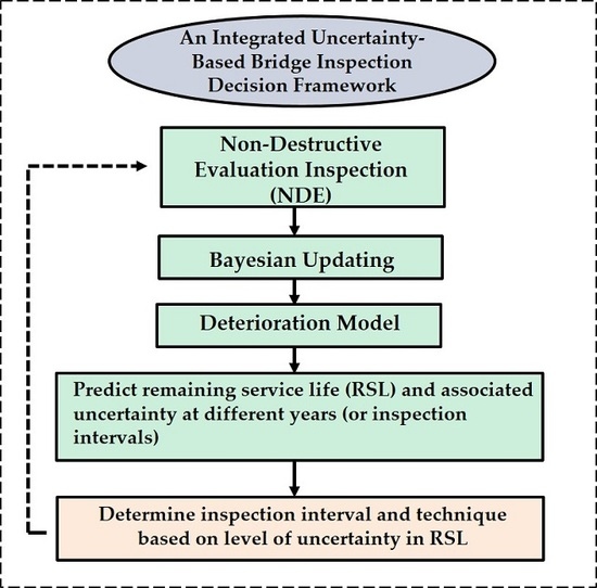
Inspection planning consists of three main steps: non-destructive inspection, the Bayesian updating process, and deterioration prediction. The inspection step involves measuring model parameters onsite using non-destructive methods. Bayesian updating is used to update the model parameters integrating the new measured data. In the deterioration prediction step, the extent of a certain deterioration stage and the probability of transitioning to a subsequent stage are estimated using models appropriate for the current state of the bridge. Using the predicted bridge condition and the uncertainty in that condition over time, the inspection time ($t_{insp}$) for the next inspection is determined.

5.3.1. Initiation of Deck Life Span at $t_0$

In this example, we consider a new bridge deck (either part of a new bridge, or a recently reconstructed deck). For demonstration purposes, it is assumed that the concrete bridge deck life span starts once chlorides have started to arrive on the surface. An early visual inspection is assumed to occur confirming construction, but no information is collected to aid in deterioration modeling. All the predicted time spans for a certain deterioration stage will be calculated from $t_0$. For example, the time until corrosion initiation $t_1$ will be the number of years starting at $t_0$.

5.3.2. Inspection Planning at $t_{insp}=2years$, (1st NDE Inspection, 1st Prediction, RSL Estimation and Choosing the Next Inspection Time ($t_{insp}$))

The first NDE inspection is assumed to be conducted after 2 years from initiation of the bridge deck life span. The two-year period is selected to reflect current bridge inspection practice. This initial period ensures that there are useful parameters to measure at the time of the first NDE inspection.

In this simulated inspection, two parameters were measured: the surface chloride concentration using a Chloride Ion Penetration test (CIP) and the concrete cover using a Pachometer. In this case, the measured surface chloride concentration ($C_0$) had a mean value of 3.5 kg/m³ and a c.o.v equal 0.5 kg/m³. The cover mean value was 6 cm and the c.o.v was 0.2 cm. These measured parameters, along with random variables representing the diffusion coefficient (D) and critical chloride concentration ($C_{th}$), shown in

Table 2. Random variables used in Monte Carlo Simulation of concrete deck deterioration.

$\mathrm{Parameter}(\mathsf{\theta })$	Mean	Coefficient of Variation (c.o.v)	Distribution	Reference
$C_0$	3.5 kg/m3	0.5	Lognormal	[14]
D	6.3 × 10−5 m2/yr.	0.75	Lognormal	[14]
$C_{th}$	1 kg/m3	0.1	Lognormal	[54]
Cover (x)	60 mm *	0.2	Lognormal	[54]
Db	18 mm *	0.02	Lognormal	[54]
Fc’	45 Mpa. *	0.18	Lognormal	[55]
w/c	$\raisebox{1ex}{$27$}\!\left/ \!\raisebox{-1ex}{$F_C\prime +21$}\right.$			[12]

* The mean values are based on the assumed design, while the c.o.v comes from cited references.

, were then used in the first prediction at $t=2years$. It should be noted that to ensure a non-destructive inspection procedure, the CIP test was used to measure only the surface chlorides, and therefore would require a relatively small sample or core from the concrete deck. However, an agency could decide to measure the chloride content at a certain depth using a more destructive method and calibrate the model in Equation (10) depending on its measurements.

Monte Carlo Simulation (MCS) was used to predict the mean and standard deviation of the RSL at different time intervals. Using the parameters measured from the inspection and assumed from the concrete properties including their associated uncertainties, the time interval to reach a specific mean chloride concentration at the rebar level was predicted using the corrosion initiation prediction model Equation (11). Using specified distributions for the chloride concentration and calculating the time to reach that chloride concentration allows estimation of uncertainty in the RSL in years. For instance, a mean chloride content of 0.6 kg/m³ will accumulate at the rebar level after almost 16 years from the arrival of chlorides on the concrete surface $(t_0)$, as shown in

Table 3. Mean and Standard Deviations of predicted time to reach specified chloride content at the rebar level used to establish the Standard deviation of RSL $({\sigma }_{T_{RSL}})$ with time (predictions at $t_{insp}=2years$).

Mean Chloride Content (kg/m3)	Time (Mean) (Years)	$\mathit{\sigma }={\mathit{\sigma }}_{{\mathit{T}}_{\mathit{R}\mathit{S}\mathit{L}}}$ (Years)
0.1	5.1	1.6
0.2	8	2.3
0.4	11.8	2.8
0.6	15.9	3.7
0.8	20.8	5.4
1	27	7

. The 16-year predicted time is associated with a standard deviation $(\sigma =3.7years)$, which corresponds to the standard deviation of the RSL $({\sigma }_{T_{RSL}})$ at year 16.

In this example, the condition threshold $y_k$ in Stage 1 is the corrosion initiation time and it is assumed to initiate at a critical chloride concertation ($C_{th}$) of 1 kg/m³ (c.o.v. = 0.1 kg/m³) [54,56]. Accordingly, using the mean and standard deviation for the time to reach a chloride content of 1 kg/m³ the probability of corrosion initiation $P_k(t)$ was estimated at different times, as indicated in

Table 4. Probability of corrosion initiation $(P_k(t))$ predicted at different times measured from $t_0$ (predictions at $t_{insp}=2years$).

Time (Years)	${\mathit{P}}_{\mathit{k}}(\mathit{t})$
20	15%
22	27%
24	40%
26	54%
27	60%
30	75%

.

The prediction made at $t_{insp}=2years$ indicates that the chloride content is expected to reach 1 kg/m³ at the rebar level after almost 27 years from the arrival of the chlorides on the concrete surface $(t_0)$ and therefore corrosion is predicted to initiate around this time. In addition, at $t_{insp}=2years$, the duration of Stage 2 was estimated to be 7 years using the variables in Table 2 and Equation (12). At year 2, Bayesian updating was not performed, since it is the first prediction, with no prior knowledge of the values of the model parameters.

In this example, the RSL is the summation the time spans of Stage 1 $(t_1)$, Stage 2 $(t_2)$ and Stage 3 $(t_3)$. The first prediction at $t=2years$ predicted that the mean value for the durations of Stage 1 and Stage 2 from $t_0$ are 27 and 7 years, respectively. A concrete bridge deck is estimated to have a life span ranging from 40 to 60 years [57,58]. In this example, the life span of the concrete bridge deck was initially assumed to be 50 years. Based on the hypothetical 50-year life span and the first deterioration prediction, the time span for Stage 3 will be 16 years ($50-27-7=16years$). Therefore, the RSL calculated at year 2 has a mean value of 48 years (i.e., ${\mu }_{T_{RSL}}(t=2)=48years$). This was calculated by adding the mean value for the predicted time span of Stage 1 (27-years), to Stage 2 (7 years) and 3 (16 years), then deducting the 2 years that have elapsed from $t_0$. This indicates that the bridge deck RSL has a mean value of 48 years, before reaching the end of its service life (as decided by the agency due to excessive cracking). However, based on the results from the first prediction, the estimated RSL is associated with uncertainty. The predicted duration of Stage 1 has a standard deviation of almost ${\sigma }_{T_{RSL}}(t=2)\approx 7years$. It is noted that the only uncertainty considered when making predictions in Stage 1 is the uncertainty associated with the predicted duration for Stage 1, while the time spans of Stage 2 and 3 are considered constant until reaching Stage 2. Using the proposed inspection process will help in reducing this degree of uncertainty in RSL, as will be demonstrated.

To choose the time interval for the next inspection, three governing factors were considered: (1) a maximum time of 6 years between inspections (i.e., $T_{\max }=6$), (2) the standard deviation of the RSL ${\sigma }_{T_{RSL}}$ exceeds 2 years (i.e., ${\sigma }_{ub}=2years$), and (3) the probability of corrosion initiation exceeding 40% (i.e., $P_k^{ub}=0.4$). Once any of the thresholds is reached, an inspection should be conducted. In practice, these thresholds should be decided by the agency or the bridge management team based on their management needs, and these thresholds could change over time as the agency became more familiar with this inspection planning process. In this example, 2 years was selected as the standard deviation threshold so as not to introduce too much uncertainty into short term budget planning. The probability threshold $P_k^{ub}$ of 40% was chosen as a way to check on the bridge before the mean expected time for corrosion to initiate. An agency might decide that they were not interested in catching corrosion initiation at very early stages and they would prefer to wait until the probability of corrosion was 80% or 90% before conducting an inspection. This demonstrates the flexibility of the proposed inspection planning process and how it can be tailored to a specific agency’s needs and budget.

The first prediction results in Table 4 show that the probability $P_k(t)$ will reach 40% after 24 years, whereas, regarding the standard deviation criterion, the next inspection should be conducted at year 8 (measured from $t_0$) when a standard deviation exceeding 2 years has been reached, and which happens to correspond to the 6 years maximum interval between inspection (with the previous inspection conducted at year 2). Thus, the next inspection will be conducted at $t_{insp}=8years$, and CIP and Pachometer non-destructive methods will be used as the bridge deck is still expected to be in Stage 1.

5.3.3. Inspection Planning at $t_{insp}=8years$, (2nd NDE Inspection, Bayesian Updating of Parameters, 2nd Prediction, RSL Estimation, and Choosing the Next Inspection Time ($t_{insp}$))

To continue the demonstration example, another simulated inspection is assumed at year 8. A Pachometer and CIP were once again used to measure the concrete cover and the surface chloride content, respectively. The simulated inspection finds the surface chloride content ($C_0$) higher than the previous measured amount at $t_{insp}=2years$ by 5% and the cover is less than the design value by the same percentage. For simplicity in this example the standard deviation of the measured surface chlorides and concrete cover were assumed to depend only on the accuracy and error factor of the equipment; since no inspection measurements or data from calibration of an NDE technique were available (i.e., refer to Equations (3) and (4), ${\beta }_1=0$ and ${\beta }_2=1$). However, in reality, the accuracy of the inspection can also depend on the proficiency of the inspectors, the number of measurements conducted and the dispersion between measurements.

In the Bayesian updating process, the measured parameter values and associated uncertainty at year 2 correspond to the prior $\mathsf{\theta }$, while the new measured values at year 8 correspond to the data. Using both sets of information, a posterior mean and standard deviation for the surface chloride concentration and concrete cover were calculated using Bayesian updating. Table 8 at the end of the example summarizes the values of the updated bridge deck parameters at each inspection time investigated.

Using samples from the posterior distribution for the bridge deck parameters, along with samples for the other Stage 1 model parameters, MCS was used for the second prediction.

Table 5. Mean and Standard Deviations of predicted time to reach specified chloride concentrations at the rebar level used to establish the Standard deviation of RSL $({\sigma }_{T_{RSL}})$ with time (predictions at $t_{insp}=8years$).

Chloride Content (kg/m3)	Time (Mean) (Years)	$\mathit{\sigma }={\mathit{\sigma }}_{{\mathit{T}}_{\mathit{R}\mathit{S}\mathit{L}}}$ (Years)
0.4	11.3	2.2
0.6	14.5	2.9
0.8	19.2	3.6
1	24.3	4.6

and

Table 6. Probability of corrosion initiation $(P_k(t))$ predicted at different times measured from t₀ (predictions at $t_{insp}=8years$).

Time (Years)	${\mathit{P}}_{\mathit{k}}(\mathit{t})$
20	17%
22	34%
23	42%
24	52%
27	78%
30	90%

show the second prediction results.

The results of the second prediction at $t_{insp}=8years$ using the updated parameters show that the expected time for corrosion initiation was reduced from 27 to 24.3 years and the standard deviation of the expected corrosion initiation time decreased to almost 4.6 years rather than 7 years. Based on the hypothetical 50-year life span of the bridge deck, the RSL after 8 years should be equal to 42 years. However, due to the simulated inspection measurements and the second prediction at year 8, the mean RSL decreased by 3 years to be 39 years (i.e., ${\mu }_{T_{RSL}}(t=8)=39years$), associated with a standard deviation ${\sigma }_{T_{RSL}}(t=8)\approx 4.6years$. This shows that updating the model parameters using the inspection results had the desired effect of decreasing the level of uncertainty (i.e., decrease in the standard deviation) associated with the prediction of deterioration and RSL estimation.

Applying the same inspection planning criteria to year 8, the results in Table 5 show that based on the standard deviation criterion, the next inspection should be conducted at year 11, which corresponds to a 3-year interval between inspections. On the other hand, based on the probability $P_k(t)$, the next inspection should be done at year 23. Therefore, the next inspection was assumed to be conducted at year 11.

5.3.4. Subsequent Inspections in Stage 1

The same procedures (inspection with CIP and Pachometer, Bayesian updating of model parameters, prediction of RSL) were applied to determine the remaining inspections needed in Stage 1. Three more inspections are needed at year 11, 14 and 18.

Table 7. Summary of all inspections in Stage 1.

Time (tinsp) (Year)	Inspection	NDE Methods Used	Prediction	Predicted Corrosion Initiation Time (years)	${\mathit{\mu }}_{{\mathit{T}}_{\mathit{R}\mathit{S}\mathit{L}}}$ (Years)	${\mathit{\sigma }}_{{\mathit{T}}_{\mathit{R}\mathit{S}\mathit{L}}}$ (Years)
2	1st NDE	CIP and Pachometer	1st prediction (using inspection results directly)	27	48	7
8	2nd NDE	CIP and Pachometer	2nd prediction (Bayesian Updating Conducted)	24	39	4.6
11	3rd NDE	CIP and Pachometer	3rd prediction (Bayesian Updating Conducted)	23.6	35.6	4.0
14	4th NDE	CIP and Pachometer	4th prediction (Bayesian Updating Conducted)	23.2	32.2	3.8
18	5th NDE	CIP and Pachometer	5th prediction (Bayesian Updating Conducted)	23.0	28	3.2
23	1st NDE in Stage 2	HCP and Polarization Resistance	1st prediction for Stage 2 (Bayesian Updating Conducted)	Corrosion initiates now	16	Depends on Stage 2 modeling

summarizes all the inspections needed in Stage 1 and the results of deterioration predictions after each inspection. It should be noted that for the conditions assumed in this example, selection of the inspection time was governed mainly by the standard deviation of 2 years at all inspection intervals. In the prediction made at year 18, it was estimated that corrosion would initiate at year 23 with a standard deviation of 3.2 years and a probability of corrosion initiation $P_k(t)$ equal to 47%, compared to a 30% probability at year 22. Therefore, based on the discussed criteria, year 23 can be considered a suitable time for performing the next inspection and to be an accepted estimation for the end of Stage 1 and the beginning of Stage 2 (active corrosion stage), which will be discussed in the next section.

Table 8. Parameters used in Stage 1 and Bayesian updating.

Year	Parameter	Parameters Based on Previous Knowledge (Prior θ)		Measured Values from Inspections (Data)		Updated Parameter Values (Posterior)
		Mean	σ	Mean	σ	Mean	σ
2	Cover (cm)			6	0.2
	Surface chloride content (kg/m3)			3.5	0.5
8	Cover (cm)	6	0.2	5.7	0.85	5.98	0.194
	Surface chloride content (kg/m3)	3.5	0.5	3.67	0.25	3.66	0.22
11	Cover (cm)	5.98	0.194	5.7	0.85	5.98	0.188
	Surface chloride content (kg/m3)	3.66	0.22	3.7	0.25	3.7	0.16
14	Cover (cm)	5.98	0.188	5.7	0.85	5.98	0.16
	Surface chloride content (kg/m3)	3.7	0.16	3.75	0.25	3.72	0.13
18	Cover (cm)	5.98	0.16	5.7	0.85	5.98	0.14
	Surface chloride content (kg/m3)	3.72	0.13	3.75	0.25	3.74	0.1

shows the values of the measured concrete deck parameters used in the deterioration model at each step in Stage 1. It also demonstrates how Bayesian updating changes the values of the parameters. It was assumed at year 11 and 14 that a slight increase in the surface chloride concentration was measured during inspection, and then the surface chloride concentration remained almost constant.

5.4. Uncertainty-Based Inspection Planning for Stage 2

Inspection Planning at $t_{insp}=23years$, (NDE Inspection, Bayesian Updating of Parameters, Prediction, RSL Estimation, and Choosing the Next Inspection Time ($t_{insp}$))

Year 23 marks the end of Stage 1 and the start of Stage 2. In Stage 2, the condition threshold $y_k$ is the time for cracking to initiate. For demonstration purposes, a half-cell potential (HCP) test was assumed to be used at this time to measure the probability of corrosion and to confirm the initiation of corrosion propagation in the rebar. The HCP recorded high probability of corrosion, which indicates the start of Stage 2. In addition, Polarization Resistance was conducted to measure the corrosion current density ($i_c)$ at year 23. When the duration of Stage 2 was initially predicted (at $t=2years$), the corrosion current density was estimated to have a mean value of 1.7 µA/cm² and a standard deviation equal to 0.1 µA/cm² obtained from Equation (14). The corrosion current density depends on the compressive strength of the concrete, water cement ratio and the concrete cover. However, the simulated non-destructive test found the corrosion current density to have a mean value equal to 2.50 µA/cm² and a standard deviation equal 0.75 µA/cm² based on the equipment accuracy representing concrete in poor condition [55].

The NDE inspection and the empirical Equation (14) used to measure and calculate the corrosion current density respectively, are associated with a degree of error or uncertainty. Therefore, to have a better estimation of the corrosion current ($i_c)$ Bayesian updating was conducted. Using the 1.7 µA/cm² as a prior value and the 2.5 µA/cm² as the collected data, Bayesian updating calculated the posterior value of the corrosion current density, which has a mean of 1.95 µA/cm² and σ = 0.12 µA/cm². This estimated value represents a better prediction for the ($i_c)$, which will improve the second Stage 2 prediction at year 23. The second prediction in Stage 2 estimated the mean crack initiation time to be after 6 years rather than 7 years from the corrosion initiation time with a standard deviation equal to 0.33 years and a probability of crack initiation $P_k(t)$ equal to 50%. Therefore, the appropriate time for the next inspection should be at year 29, which is 6 years after the corrosion initiation and also corresponds to the maximum time between inspections (i.e., $T_{\max }=6$). The inspection techniques that should be used at year 29 should be able to detect cracks (e.g., GPR, IE or Chain drag). Their results can be used to confirm that Stage 3 has started and cracks are propagating in the concrete deck.

Based on the first estimation of the predicted duration of Stage 2 (7 years), the mean RSL calculated is ${\mu }_{T_{RSL}}(t=2)=23years$ with a standard deviation ${\sigma }_{T_{RSL}}(t=2)=0.5years$. This is calculated by adding the estimated duration of Stage 2 (7 years) and Stage 3 (16 years), While based on the NDE inspection done at 23-years, which resulted in a new estimated active corrosion time equal 6 years, the new estimated mean RSL will equal ${\mu }_{T_{RSL}}(t=23)=22years$ with a standard deviation ${\sigma }_{T_{RSL}}(t=23)=0.3years$. Figure 5 summarizes the inspection planning process for Stage 1 and 2. Note that in general, there is a discontinuity in the predicted RSL at the time of each inspection. The discontinuity occurs as the deterioration model is updated with new inspection results. In this example, the assumed inspection findings were always a little more severe than the anticipated findings, resulting in the shorter RSL. If the assumed inspection findings had been less severe than anticipated, the RSL would have increased at the time of the inspection. Overall, the deterioration paths and inspection results in Figure 5 correspond to a specific realization of the inspection planning process. When the framework is applied in real-life, the inspection data or the sequence of inspection data may or may not have fluctuations and the corresponding inspection process will depend on the actual data which could be different for each bridge. In addition, note that the deterioration paths are smooth because they corresponds to mean predictions from the deterioration model rather than the measured deterioration path based on inspection data, which will have fluctuations.

5.5. Discussion of Inspection Planning Results

Given the assumptions made in the example, using the proposed inspection planning process specified, only five inspections need to be conducted in the 23-year Stage 1 period compared to 11 inspections if the standard 2 year inspection interval was implemented. In Stage 2, using the proposed inspection plan resulted in two inspections in a 6-year period compared to 3. It should be acknowledged that NDE-based inspections might require an initial capital cost to obtain equipment and train NDE personnel. However, these initial capital costs would be distributed over all bridges under management and over the total life span of a bridge deck. The use of NDE is expected to provide better information than visual inspections and the reduced number of required inspections should make NDE inspections at least cost-competitive if not cost-saving when compared to visual inspections.

In this example, two stages in a concrete bridge deck life span were investigated. The proposed inspection planning framework is flexible and can be tailored to different types of bridge construction (materials and techniques) by establishing appropriate bridge service life Stages and corresponding NDE techniques for other types of bridges and bridge elements. The method can be further adapted to different agency decision-making practices and objectives through careful selection of allowable levels of uncertainty and probabilities of Stage transition. In the effort to keep the example straightforward, some subtleties were not fully described previously. For example, during the analysis, it was observed that if more deterioration model parameters are measured on site and updated, the proposed inspection planning framework will be more effective. For example, if the diffusion coefficient (D) was measured on site and the inspection value was then used in Bayesian updating, this would have resulted in a different outcome, since the uncertainty regarding the diffusion coefficient would decrease. If, for example, the measured diffusion coefficient was found to be 5% higher than assumed, the corrosion initiation time initially predicted would have changed from 27 years to 23.4 years and the standard deviation (${\sigma }_{T_{RSL}}(t))$ would have decreased by 3.4 years rather than 2.4 years only, which would reduce the number of inspections in Stage 1 to four NDE inspections rather than five.

However, there has not yet been any reliable data regarding a non-destructive test that can be used to measure the diffusion coefficient. If an agency wanted to enhance its predictions, the agency could choose to perform a destructive test on the bridge deck in the early inspections to have a better estimation of the diffusion coefficient of the concrete material or to measure the chloride content at the rebar level and compare it with the estimated value. The agency would need to consider the costs and damage caused by destructive testing and the potential value of enhanced deterioration predictions.

In addition, the Bayesian updating process can be affected by the accuracy of the inspection technique or equipment used. For example, the CIP test was found to have an error factor ±0.25 kg/m³, and this error factor resulted in a standard deviation of 4.6 years (as can be seen in Table 5) when predicting the corrosion initiation time. In contrast, if this error factor was ±0.5 kg/m3, the standard deviation would have become 5.2 years. This shows that using more accurate techniques in the inspection can help to decrease the level of uncertainty. As explained in earlier sections, a target uncertainty level can be chosen and a suitable inspection technique with higher accuracy that can decrease the level of uncertainty to the target level could be selected. However, this might come with a higher cost, since using more accurate inspection techniques might require more time and money. A subsequent economic analysis is needed to investigate the trade-offs of using more expensive but more accurate NDE methods.

6. Conclusions and Future Research

This paper presents a new approach to inspection planning of bridges (both the timing and the type of inspection) integrating NDE inspection findings and deterioration model predictions by considering uncertainty in bridge condition (measured with the RSL). In the proposed approach, inspections are viewed not only as a means to evaluate the amount of deterioration in the bridge and thus reduce the uncertainty in our current knowledge of the condition of a bridge, but also as a way of updating the deterioration models that will predict future condition. By incorporating deterioration models as an additional source of information about bridge condition, inspections can be conducted less frequently. Using deterioration models to predict the Stage of bridge service life and the need to reduce uncertainty to acceptable levels provides a means to justify the use of particular inspection processes for a given bridge.

Conducting inspections only when the information collected can be used to reduce uncertainty in bridge condition and enhance information for decision-making can help optimize agency resources and reduce bridge management costs significantly.

The proposed framework is demonstrated through application of a newly constructed reinforced concrete bridge deck with time until crack appearance as RSL. Deterioration models were used to predict the time of corrosion initiation and propagation. Inspection scenarios where NDE equipment were used to update model parameters were simulated. Then, Bayesian updating was used to estimate the bridge deck RSL and to determine the time of the next inspection interval. Due to the flexibility of the proposed framework, two criteria were used to choose the inspection time; the standard deviation (i.e., amount of uncertainty) associated with estimated RSL and the probability of reaching a certain deterioration stage. NDE methods were chosen based on the deterioration stage, the required model parameters to be updated and the equipment level of accuracy.

For the bridge used in the example, the proposed inspection process helped in reducing the number of inspections to 5 in Stage 1 and 2 in Stage 2 compared to the traditional two-year visual inspection cycles which would have resulted in 11 and 3 inspections, respectively. When considered in the context of a network of bridges, potential savings are much more significant. Based on the current analysis, updating more model parameters during inspection measurements will further reduce uncertainty associated with the estimated RSL. The proposed framework helps in determining the suitable equipment (NDE method) for the next inspection, offers flexibility to agencies to set criteria appropriate to their management practices and required level of certainty, and reduces the number of inspections during a certain deterioration stage. This significantly assists in the bridge management process and inspection decision making.

While significant development remains before practical application, this paper demonstrates a novel approach to the timing of bridge inspections that makes use of deterioration models to reduce the required frequency of inspections and helps decide the type of inspection that should be conducted.

Note that the focus of this paper is on mathematically formulating the uncertainty-based bridge inspection framework. The application to reinforced concrete bridge deck was used as an example. However, the proposed framework is generic and can be applied to different bridge types (e.g., concrete bridges, steel bridges) and different bridge conditions (e.g., newly-constructed bridges, in-service bridges), in which cases appropriate deterioration models and corresponding inspection techniques, as well as definition of RSL need to be used. While the maintenance is not explicitly modeled in the framework, one potential way to incorporate maintenance action is by (1) updating the (initial) condition and associated uncertainties after the maintenance action, and (2) using corresponding deterioration models that can include the maintenance effects (e.g., if the maintenance corresponds to a replacement, then the deterioration model for new elements should be used; if the maintenance corresponds to some repair, then the deterioration model for repaired elements should be used). On the other hand, to fully leverage the proposed framework, developments and advancements in deterioration models (e.g., those that can incorporate the effects of maintenance actions) and systematic interpretation and incorporation of results from different NDE inspection techniques (e.g., GPR, IE, and others) would be needed. These represent current research areas in the bridge management domain. The framework introduced herein contributes to the body of knowledge by focusing on inspection planning in particular (a topic studied less often than maintenance planning) and proposing a new direction to bridge inspection decision making. The framework has the potential to complement and benefit from the ongoing research in the bridge management domain. As such, it is likely to promote more discussion and research on this important topic.

There are many avenues for further development of the planning framework. Future research should focus on studying the impact of the proposed inspection planning framework on the life cycle cost of a bridge, particularly when compared with other inspection programs. Implementing the proposed approach on existing bridges and including the effect of any maintenance actions performed on the bridge deck in the inspection framework should be studied. Mitigating risk in asset management is approached differently by each agency, the effect of the proposed approach on risk analysis in a bridge network can be analyzed and compared with different approaches. Bridge inspection has a significant effect on bridge maintenance, and the effect of the proposed inspection planning should be analyzed from different stand points, such as economic and environmental consequences of maintenance. The optimization of resources can also be implemented on the whole bridge network of an agency, for example, NDE inspections can be applied on critical bridges only to avoid budget deficiency. The effect of implementing such approach on the bridge network budgeting should be investigated.

References

1. Dorafshan, S.; Maguire, M. Bridge inspection: Human performance, unmanned aerial systems and automation. J. Civ. Struct. Health Monit. 2018, 8, 443–476. [Google Scholar] [CrossRef]
2. FHWA. Bridge Inspector’s Reference Manual, Vol. 1; Federal Highway Administration: Washington, DC, USA, 2012.
3. Briaud, J.-L.; Hunt, B. Bridge scour and the structural engineer. Struct. Dec. 2006, 58–61. [Google Scholar]
4. ASCE/SEI-AASHTO Ad-Hoc Group on Bridge Inspection, Rating, Rehabilitation and Replacement. White Paper on Bridge Inspection and Rating; American Society of Civil Engineers: Reston, VA, USA, 2009. [Google Scholar]
5. FHWA. Recording and Coding Guide for the Structure Inventory and Appraisal of the Nations Bridges; Federal Highway Administration: Washington, DC, USA, 1995.
6. AASHTO. Guide for Commonly Recognized (CoRe) Structural Elements; AASHTO: Washington, DC, USA, 1998. [Google Scholar]
7. Thompson, P.D.; Shepard, R.W. AASHTO Commonly-recognized bridge elements. In Materials for National Workshop on Commonly Recognized Measures for Maintenance, Scottsdale, Arizona. 2000. Available online: https://pdfs.semanticscholar.org/da6c/3017e1396056cf500ee587601d9bce2bb3dc.pdf (accessed on 20 May 2019).
8. Gucunski, N.; Pailes, B.; Kim, J.; Azari, H.; Dinh, K. Capture and quantification of deterioration progression in concrete bridge decks through periodical NDE surveys. J. Infrastruct. Syst. 2016, 23, B4016005. [Google Scholar] [CrossRef]
9. Lee, S.; Kalos, N. Non-destructive testing methods in the US for bridge inspection and maintenance. KSCE J. Civ. Eng. 2014, 18, 1322–1331. [Google Scholar] [CrossRef]
10. Broberg, P. Surface crack detection in welds using thermography. NDT E Int. 2013, 57, 69–73. [Google Scholar] [CrossRef]
11. Yehia, S.; Abudayyeh, O.; Nabulsi, S.; Abdelqader, I. Detection of common defects in concrete bridge decks using nondestructive evaluation techniques. J. Bridge Eng. 2007, 12, 215–225. [Google Scholar] [CrossRef]
12. Vu, K.A.T.; Stewart, M.G. Structural reliability of concrete bridges including improved chloride-induced corrosion models. Struct. Saf. 2000, 22, 313–333. [Google Scholar] [CrossRef]
13. Cheung, M.M.; So, K.K. Service Life Prediction and Management of Concrete Bridge Structures Due to Corrosion. J. Civ. Eng. Archit. 2015, 9, 1153–1166. [Google Scholar]
14. Stewart, M.G.; Rosowsky, D.V. Time-dependent reliability of deteriorating reinforced concrete bridge decks. Struct. Saf. 1998, 20, 91–109. [Google Scholar] [CrossRef]
15. Cady, P.D.; Weyers, R.E. Chloride penetration and the deterioration of concrete bridge decks. Cem. Concr. Aggreg. 1983, 5, 81–87. [Google Scholar]
16. Chryssanthopoulos, M.; Sterritt, G. Integration of deterioration modelling and reliability assessment for reinforced concrete bridge structures. In Proceedings of the Asranet International Colloquium, Glasgow, Scotland, 8–10 July 2002. [Google Scholar]
17. Val, D.V.; Stewart, M.G.; Melchers, R.E. Life-cycle performance of RC bridges: Probabilistic approach. Comput. Aided Civ. Infrastruct. Eng. 2000, 15, 14–25. [Google Scholar] [CrossRef]
18. Scherer, W.T.; Glagola, D.M. Markovian models for bridge maintenance management. J. Transp. Eng. 1994, 120, 37–51. [Google Scholar] [CrossRef]
19. Morcous, G.; Rivard, H.; Hanna, A. Modeling bridge deterioration using case-based reasoning. J. Infrastruct. Syst. 2002, 8, 86–95. [Google Scholar] [CrossRef]
20. Mishalani, R.G.; Shafieezadeh, A.; Li, Z. Updating Bridge Deck Condition Transition Probabilities as New Inspection Data Are Collected: Methodology and Empirical Evaluation. Transp. Res. Rec. 2018, 2672, 93–102. [Google Scholar] [CrossRef] [Green Version]
21. Mizutani, D.; Lethanh, N.; Adey, B.T.; Kaito, K. Estimating Markov Transition Probabilities for Reinforced Concrete Structures Using Mechanistic-Empirical Models. 2017. Available online: https://trid.trb.org/view/1437767 (accessed on 18 July 2019).
22. Biondini, F.; Frangopol, D.M. Life-cycle performance of deteriorating structural systems under uncertainty. J. Struct. Eng. 2016, 142, F4016001. [Google Scholar] [CrossRef]
23. Baik, H.-S.; Jeong, H.S.; Abraham, D.M. Estimating transition probabilities in Markov chain-based deterioration models for management of wastewater systems. J. Water Resour. Plan. Manag. 2006, 132, 15–24. [Google Scholar] [CrossRef]
24. Torres-Luque, M.; Bastidas-Arteaga, E.; Schoefs, F.; Sánchez-Silva, M.; Osma, J.F. Non-destructive methods for measuring chloride ingress into concrete: State-of-the-art and future challenges. Constr. Build. Mater. 2014, 68, 68–81. [Google Scholar] [CrossRef] [Green Version]
25. Choe, D.-E.; Gardoni, P.; Rosowsky, D.; Haukaas, T. Seismic fragility estimates for reinforced concrete bridges subject to corrosion. Struct. Saf. 2009, 31, 275–283. [Google Scholar] [CrossRef]
26. Lindvall, A. Duracrete–probabilistic performance based durability design of concrete structures. In Proceedings of the 2nd Int. PhD. Symposium in civil engineering, Budapest, Hungary, 28–30 May 1999. [Google Scholar]
27. Ghosh, J.; Padgett, J.E. Aging considerations in the development of time-dependent seismic fragility curves. J. Struct. Eng. 2010, 136, 1497–1511. [Google Scholar] [CrossRef]
28. Li, Q.; Wang, C.; Ellingwood, B.R. Time-dependent reliability of aging structures in the presence of non-stationary loads and degradation. Struct. Saf. 2015, 52, 132–141. [Google Scholar] [CrossRef]
29. Van Noortwijk, J.M. A survey of the application of gamma processes in maintenance. Reliab. Eng. Syst. Saf. 2009, 94, 2–21. [Google Scholar] [CrossRef]
30. Peng, W.; Li, Y.-F.; Yang, Y.-J.; Huang, H.-Z.; Zuo, M.J. Inverse Gaussian process models for degradation analysis: A Bayesian perspective. Reliab. Eng. Syst. Saf. 2014, 130, 175–189. [Google Scholar] [CrossRef]
31. Bocchini, P.; Saydam, D.; Frangopol, D.M. Efficient, accurate, and simple Markov chain model for the life-cycle analysis of bridge groups. Struct. Saf. 2013, 40, 51–64. [Google Scholar] [CrossRef]
32. Jia, G.; Gardoni, P. State-dependent stochastic models: A general stochastic framework for modeling deteriorating engineering systems considering multiple deterioration processes and their interactions. Struct. Saf. 2018, 72, 99–110. [Google Scholar] [CrossRef]
33. Kallen, M.; Van Noortwijk, J. Statistical inference for Markov deterioration models of bridge conditions in the Netherlands. In Proceedings of the Third International Conference on Bridge Maintenance, Safety and Management (IABMAS), Porto, Portugal, 16–19 July 2006; pp. 16–19. [Google Scholar]
34. Ranjith, S.; Setunge, S.; Gravina, R.; Venkatesan, S. Deterioration prediction of timber bridge elements using the Markov chain. J. Perform. Constr. Facil. 2011, 27, 319–325. [Google Scholar] [CrossRef]
35. Agrawal, A.K.; Kawaguchi, A.; Chen, Z. Deterioration rates of typical bridge elements in New York. J. Bridge Eng. 2010, 15, 419–429. [Google Scholar] [CrossRef]
36. Washer, G.; Nasrollahi, M.; Applebury, C.; Connor, R.; Ciolko, A.; Kogler, R.; Fish, P.; Forsyth, D. Propos. Guideline for Reliability-Based Bridge Inspection Practices. 2014. Available online: https://trid.trb.org/view/1326950 (accessed on 15 May 2019).
37. FHWA. Nondestructive Evaluation (NDE) Web Manual. Available online: https://fhwaapps.fhwa.dot.gov/ndep/TechniqueLocatorNew.aspx (accessed on 18 July 2019).
38. Faroz, S.A.; Pujari, N.N.; Ghosh, S. Reliability of a corroded RC beam based on Bayesian updating of the corrosion model. Eng. Struct. 2016, 126, 457–468. [Google Scholar] [CrossRef]
39. Simola, K.; Pulkkinen, U. Models for non-destructive inspection data. Reliab. Eng Syst. Saf. 1998, 60, 1–12. [Google Scholar] [CrossRef]
40. Zheng, R.; Ellingwood, B.R. Role of non-destructive evaluation in time-dependent reliability analysis. Struct. Saf. 1998, 20, 325–339. [Google Scholar] [CrossRef]
41. Hesse, A.A.; Atadero, R.A.; Ozbek, M.E. Uncertainty in common NDE techniques for use in risk-based bridge inspection planning: Existing data. J. Bridge Eng. 2015, 20, 04015004. [Google Scholar] [CrossRef]
42. AASHTO-LRFD. AASHTO LRFD Bridge Design Specifications, 8th ed.; American Association of State Highway and Transportation Officials: Washington, DC, USA, 2017. [Google Scholar]
43. Lounis, Z. Probabilistic modeling of chloride contamination and corrosion of concrete bridge structures. In Proceedings of the ISUMA 2003, College Park, MD, USA, 21–24 September 2003; pp. 447–451. [Google Scholar]
44. Vu, K.; Stewart, M.G.; Mullard, J. Corrosion-induced cracking: Experimental data and predictive models. ACI Struct. J. 2005, 102, 719. [Google Scholar]
45. Onoufriou, T.; Rafiq, M.I.; Chryssanthopoulos, M.K. Performance updating of concrete bridges using proactive health monitoring methods. Reliab. Eng. Syst. Saf. 2004, 86, 247–256. [Google Scholar]
46. Sarja, A.; Vesikari, E. Durability Design of Concrete Structures; CRC Press: Boca Raton, FL, USA, 2014. [Google Scholar]
47. Siemes, A.; Vrouwenvelder, A.; Van Den Beukel, A. Stochastic modeling of building materials performance in durability. In Problems in Service Life Prediction of Building and Construction Materials; Springer: Dordrecht, The Netherlands, 1985; pp. 253–263. [Google Scholar]
48. Roberts, M.; Atkins, C.; Hogg, V.; Middleton, C. A proposed empirical corrosion model for reinforced concrete. Proc. Inst. Civ. Eng. Struct. Build. 2000, 140, 1–11. [Google Scholar] [CrossRef]
49. Sivasubramanian, K.; Jaya, K.; Neelemegam, M. Covermeter for identifying cover depth and rebar diameter in high strength concrete. Int. J. Civ. Struct. Eng. 2013, 3, 557–563. [Google Scholar]
50. ASTM. ASTM C1218/C1218M standard test method for water-soluble chloride in mortar and concrete. In Annual Book of American Society of Testing and Materials; ASTM: West Conshohocken, PA, USA, 2008. [Google Scholar]
51. ASTM-C876-09. Standard test method for half-cell potentials of uncoated reinforcing steel in concrete. In American Society for Testing and Materials; ASTM: West Conshohocken, PA, USA, 2009. [Google Scholar]
52. Gucunski, N.; Imani, A.; Francisco, R.; Nazarian, S.; Yuan, D.; Wiggenhauser, H.; Kutrubes, D. Non-Destructive Testing to Identify Bridge Deck Deterioration; SRHP: Washington, DC, USA, 2013. [Google Scholar]
53. Standard, A. G59–97: Standard test method for conducting potentiodynamic polarization resistance measurements. Annu. Book ASTM Stand. 2009, 3, 237–239. [Google Scholar]
54. Enright, M.P.; Frangopol, D.M. Probabilistic analysis of resistance degradation of reinforced concrete bridge beams under corrosion. Eng. Struct. 1998, 20, 960–971. [Google Scholar] [CrossRef]
55. Duprat, F. Reliability of RC beams under chloride-ingress. Constr. Build. Mater. 2007, 21, 1605–1616. [Google Scholar] [CrossRef]
56. Xi, Y.; Jing, Y.; Railsback, R. Surface Chloride Levels in Colorado Structural Concrete; Colorado Department of Transportation: Denver, CO, USA, 2018.
57. Taylor, B.R.; Qiao, Y.; Bowman, M.D.; Labi, S. The economic impact of implementing nondestructive testing of reinforced concrete bridge decks in Indiana; Purdue University: West Lafayette, IN, USA, 2016. [Google Scholar]
58. Liang, M.-T.; Lin, L.-H.; Liang, C.-H. Service life prediction of existing reinforced concrete bridges exposed to chloride environment. J. Infrastruct. Syst. 2002, 8, 76–85. [Google Scholar] [CrossRef]
59. Sanders, P.; Atadero, R.; Ozbek, M. Methodology for Uncertainty-Based Inspection Planning of Concrete Bridge Decks Using Mechanistic Models of Crack Formation and Propagation; Colorado State University: Fort Collins, CO, USA, 2015. [Google Scholar]
Figure 1. Conceptual representation of increasing uncertainty about bridge condition over time, and the reduction in uncertainty resulting from updated inspection findings.
Infrastructures 04 00050 g001
Figure 2. Flowchart of the proposed uncertainty-based inspection decision framework.
Infrastructures 04 00050 g002
Figure 3. An example implementation of the uncertainty-based inspection planning (The solid lines in the figure represent the mean predicted RSL, while the dotted lines represent the uncertainty in the prediction).
Infrastructures 04 00050 g003
Figure 4. Cross-section for the example reinforced concrete deck.
Infrastructures 04 00050 g004
Figure 5. Illustration of inspection planning process for Stage 1 and Stage 2. The solid lines in the figure represent the mean RSL predicted with deterioration model, while the dotted lines represent the uncertainty in the prediction.
Infrastructures 04 00050 g005