Civil Infrastructure Management Models for the Connected and Automated Vehicles Technology

Abstract
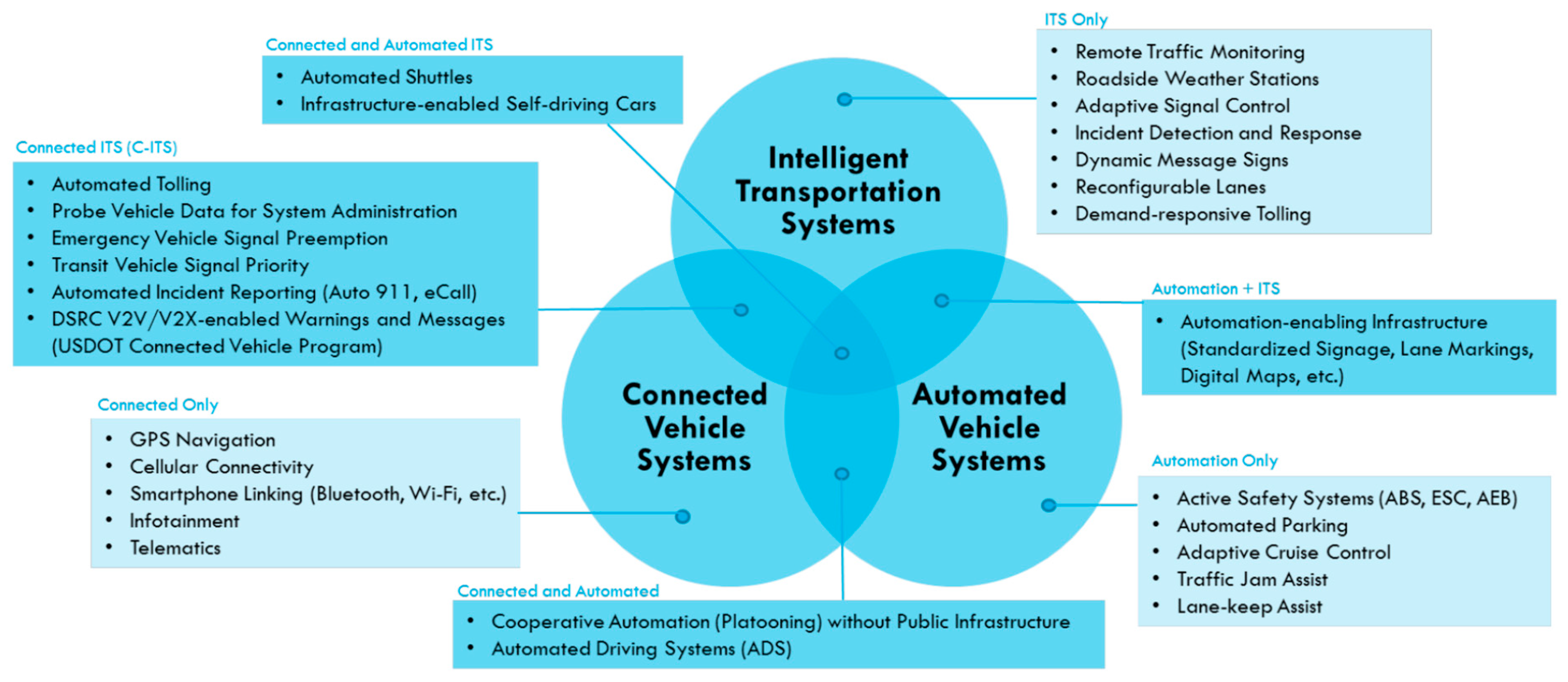
1. Introduction
- No Automation (Level 0): The driver is in complete and sole control of the primary vehicle controls—brakes, steering, throttle, and motive power—at all times.
- Function-Specific Automation (Level 1): Automation at this level involves one or more specific control functions. Examples include electronic stability control or pre-charged brakes, where the vehicle automatically assists with braking to enable the driver to retain control of the vehicle or stop faster than possible if acting alone.
- Combined Function Automation (Level 2): This level involves automation of at least two primary control functions designed to work in unison to relieve the driver of control of those functions. An example of combined functions enabling a Level 2 system is adaptive cruise control in combination with lane centering.
- Limited Self-Driving Automation (Level 3): Vehicles at this level of automation enable the driver to cede full control of all safety-critical functions under certain traffic or environmental conditions to rely on the vehicle to monitor changes in those conditions requiring transition back to driver control. The driver is expected to be available for occasional control, but with sufficient transition time. The Google car is an example of limited self-driving automation.
- Full Self-Driving Automation (Level 4): The vehicle is designed to perform all safety-critical driving functions and monitor roadway conditions for an entire trip. Such a design anticipates that the driver will provide destination or navigation input but is not expected to be available for control at any time during the trip. This includes both occupied and unoccupied vehicles. The SAE definitions further breaks the NHTSA’s Level 4 into SAE’s Level 4 (high automation) and Level 5 (full automation), as shown in Figure 2.
2. Automation of the Infrastructure
3. Infrastructure Requirements for CAVs
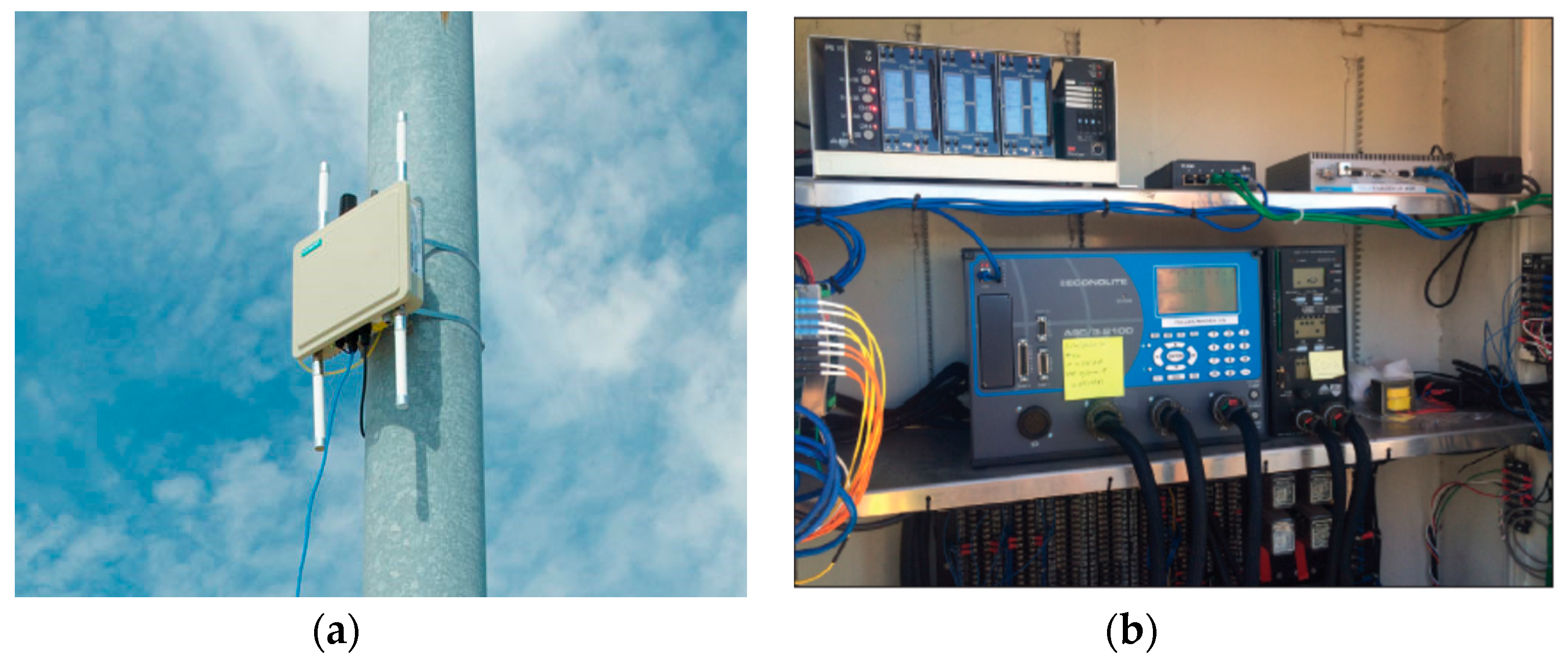
3.1. V2I Deployment Coalition
- The majority of the infrastructure needs for CAV implementation will be associated with intersections.
- There will be many mechanical types of elements and components, to be installed or constructed with the infrastructure. Thus, deterioration models will need to consider failure times and use reliability-based concepts.
- There will be a need to evaluate warranty period and repairs and (quick) replacement of failed components for RSUs.
- An appropriate technology for health monitoring may be needed for the RSUs.
3.2. Asset Management
3.3. Deployment Costs
3.4. Traffic Crash Costs
3.5. Condition Assessment and Deterioration Models
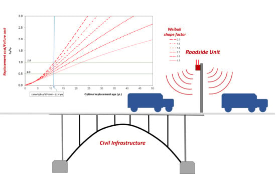
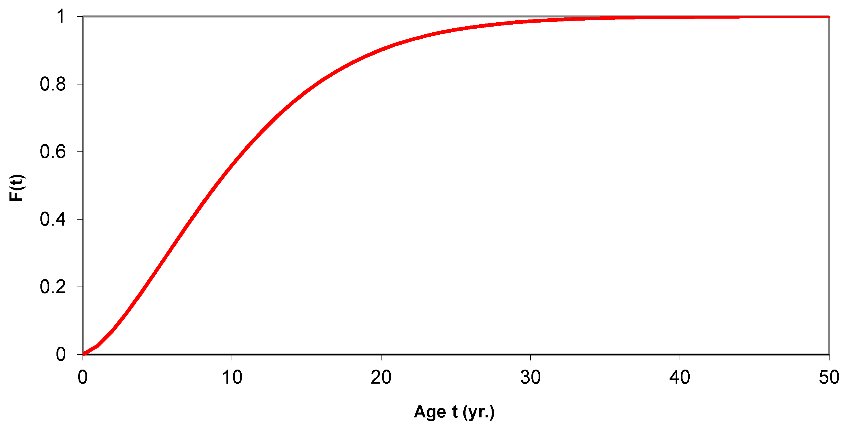
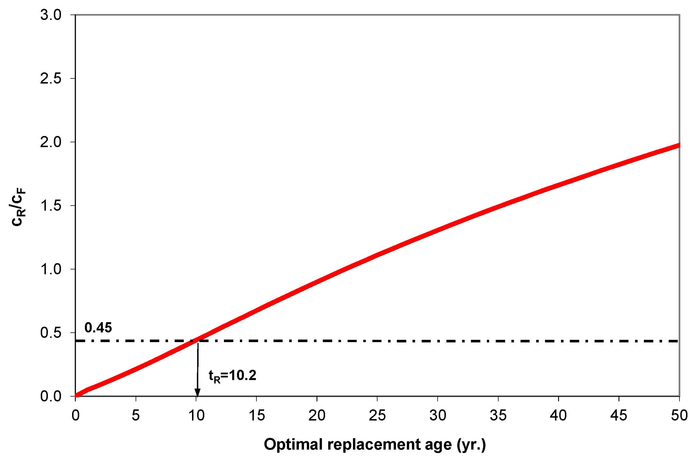
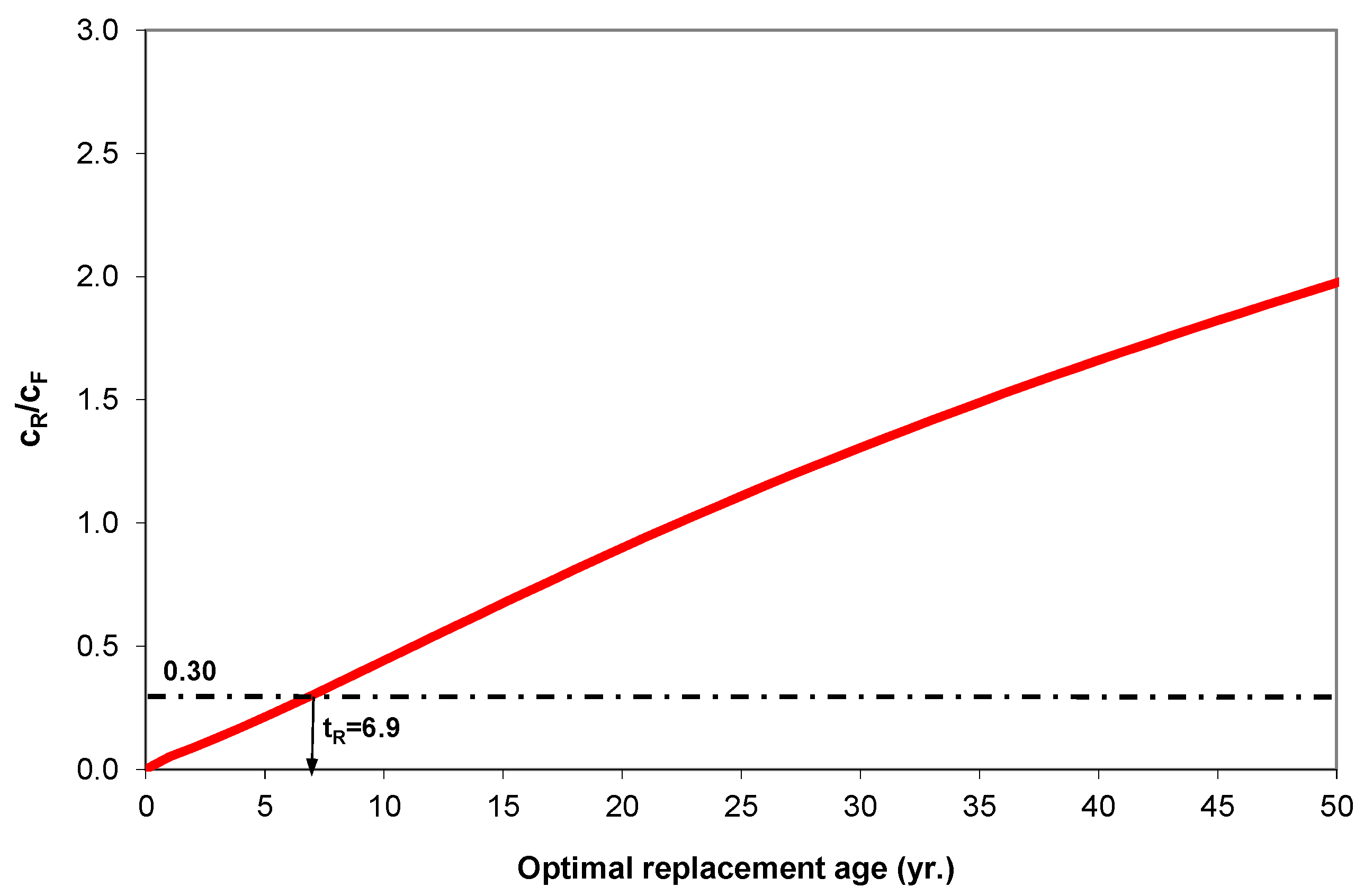
4. Age Replacement Models
Numerical Illustration
5. Other CAV Considerations
5.1. Vulnerability to Natural Hazards
5.2. User Costs Considerations
6. Conclusions
Funding
Conflicts of Interest
References
- USDOT. Connected Vehicle Basics. U.S. Department of Transportation’s (USDOT); 2018. Available online: https://www.its.dot.gov/cv_basics/ (accessed on 31 January 2018).
- NHTSA. Automated Driving Systems 2.0: A Vision for Safety. U.S. Department of Transportation (USDOT) and the National Highway Traffic Safety Administration (NHTSA), 12 September 2017. Available online: https://www.nhtsa.gov/press-releases/us-dot-releases-new-automated-driving-systems-guidance (accessed on 31 January 2018).
- PCS. Planning for Connected and Automated Vehicles. Prepared by Public Sector Consultants (PSC), Lansing, Michigan, and Center for Automotive Research, Ann Arbor, Michigan, Prepared for Greater Ann Arbor Region Prosperity Region 9. March 2017. Available online: http://www.cargroup.org/wp-content/uploads/2017/03/Planning-for-Connected-and-Automated-Vehicles-Report.pdf (accessed on 31 January 2018).
- SEMA. NHTSA, SAE Define 5 Levels of Vehicle Automation. Specialty Equipment Market Association (SEMA), eNews Volume 20, No. 11. 16 March 2017. Available online: https://www.sema.org/sema-enews/2017/11/ettn-tech-alert-nhtsa-sae-define-5-levels-of-vehicle-automation (accessed on 30 January 2018).
- Chang, J. An Overview of USDOT Connected Vehicle Roadside Unit Research Activities. Publication Number: FHWA JPO-17-433. Published May 2017. Available online: www.its.dot.gov/index.htm (accessed on 30 November 2017).
- Wright, J.; Garrett, J.K.; Hill, C.J.; Krueger, G.D.; Evans, J.H.; Andrews, S.; Wilson, C.K.; Rajbhandari, R.; Burkhard, B. National Connected Vehicle Field Infrastructure Footprint Analysis. American Association of State Highway and Transportation Officials. Technical Report No. FHWA-JPO-14-125; United States. Dept. of Transportation. ITS Joint Program Office, 27 June 2014; 235p. Available online: https://rosap.ntl.bts.gov/view/dot/3440 (accessed on 30 January 2018).
- Waldrop, M.M. No Drivers Required. Nature 2015, 518, 20–21. Available online: https://www.nature.com/news/polopoly_fs/1.16832!/menu/main/topColumns/topLeftColumn/pdf/518020a.pdf (accessed on 30 January 2018). [CrossRef] [PubMed]
- NHTSA. U.S. DOT Advances Deployment of Connected Vehicle Technology to Prevent Hundreds of Thousands of Crashes; National Highway Traffic Safety Administration (NHTSA): Washington, DC, USA, Published 13 December 2016. Available online: https://www.nhtsa.gov/press-releases/us-dot-advances-deployment-connected-vehicle-technology-prevent-hundreds-thousands (accessed on 22 January 2018).
- Hedlund, J. Autonomous Vehicles Meet Human Drivers: Traffic Safety Issues for States; Prepared for Governors Highway Safety Association: Washington, DC, USA, February 2017; 26p, Available online: https://www.ghsa.org/sites/default/files/2017-01/AV%202017%20-%20FINAL.pdf (accessed on 29 July 2019).
- General Motors. Self-Driving Safety Report: Creating New Technology to Bring New Benefits. 2018. Available online: https://www.gm.com/content/dam/company/docs/us/en/gmcom/gmsafetyreport.pdf (accessed on 29 July 2019).
- Cheon, S. An overview of Automated Highway Systems (AHS) and the Social and Institutional Challenges They Face. UC Berkeley Faculty Publications. 2003. Available online: https://escholarship.org/content/qt8j86h0cj/qt8j86h0cj.pdf (accessed on 30 November 2017).
- Zhang, Y. Adapting Infrastructure for Automated Driving; Technical Report. Prepared for Tampa Hillsborough Expressway Authority; Department of Civil and Environmental Engineering, University of South Florida: Tampa, FL, USA, November 2013; 15p. [Google Scholar]
- GAO. Vehicle-to-Infrastructure Technologies Expected to Offer Benefits, but Deployment Challenges Existing Intelligent Transportation Systems. Government Accountability Office (GAO); Published September 2015. Available online: https://www.gao.gov/assets/680/672548.pdf (accessed on 31 December 2017).
- Tampa. Connected Vehicle Demonstration, Tampa Connected Vehicle Pilot. Tampa Hillsborough Expressway Authority. Available online: https://www.tampacvpilot.com/media-resources/photos/ (accessed on 15 July 2018).
- Barbaresso, J.C.; Johnson, P. Connected Vehicle Infrastructure Deployment Considerations: Lessons Learned from the Safety Pilot Model Deployment; Report Contract No. DTFH61-11-C-00040; HNTB Corporation, for University of Michigan Transportation Research Institute: Ann Arbor, MI, USA, 30 May 2014; 49p. [Google Scholar]
- FHWA. Freeway Management and Operations Handbook. Federal Highway Administration, United States Department of Transportation. Available online: https://ops.fhwa.dot.gov/freewaymgmt/publications/frwy_mgmt_handbook/chapter15_01.htm (accessed on 20 May 2018).
- USDOT. V2I Deployment Coalition. Technical Memorandum 4: Phase 1 Final Report. Published January 2017; 174p. Available online: https://transportationops.org/V2I/V2I-overview (accessed on 30 January 2018).
- Markow, M.J. Managing Selected Transportation Assets: Signals, Lighting, Signs, Pavement Markings, Culverts, and Sidewalks; NCHRP Synthesis 371; A Synthesis of Highway Practice, Transportation Research Board: Washington, DC, USA, 2007; 199p, ISBN 978-0-309-09789-5. [Google Scholar]
- FHWA. Transportation Asset Management Case Studies (Economics in Asset Management): The Hillsborough County, Florida, Experience. United States Department of Transportation, Federal Highway Administration, Office of Asset Management, May 2005; 24p. Available online: https://www.fhwa.dot.gov/infrastructure/asstmgmt/difl.pdf (accessed on 30 January 2018).
- Sobanjo, J.; Thompson, P. Enhancement of the FDOT’s Project Level and Network Level Bridge Management Analysis Tools; Final Report, Research Contract No. BDK83 977-01; Florida Department of Transportation: Tallahassee, FL, USA, 2011; 329p. Available online: https://rosap.ntl.bts.gov/view/dot/18692 (accessed on 30 January 2018).
- US DOT. Knowledge Resources: ITS Costs Database. Intelligent Transportation Systems Joint Program Office. Department of Transportation (U.S. DOT). Available online: https://www.itscosts.its.dot.gov/its/benecost.nsf/CostHome (accessed on 15 November 2018).
- Perez, S. Tampa Offers First Demo of its Connected Vehicle Technology Project, Launching with 1,600 cars in 2018. Available online: https://techcrunch.com/2017/11/13/tampa-offers-first-demo-of-its-connected-vehicle-technology-project-launching-with-1600-cars-in-2018/ (accessed on 15 November 2018).
- Jones, J.L. Autonomous Vehicle Report; Florida Highway Safety and Motor Vehicles: Tallahassee, FL, USA, 10 February 2014; 7p. [Google Scholar]
- Gordon, R.; Cade, B. Traffic Signal Operations and Maintenance Staffing Guidelines. Prepared by Dunn Engineering Associates, P.C. in cooperation with Kittelson and Associates, Inc. Prepared for Federal Highway Administration Washington, DC, USA; March 2009; 84p. Available online: https://ops.fhwa.dot.gov/publications/fhwahop09006/fhwahop09006.pdf (accessed on 15 November 2018).
- Harmon, T.; Geni, B.; Frank, G. Crash Costs for Highway Safety Analysis. Report No. FHWA-SA-17-071, Contract or Grant No. DTFH61-16-D-00005 (VHB); Federal Highway Administration Office of Safety: Washington, DC, USA, January 2018; 120p. Available online: https://safety.fhwa.dot.gov/hsip/docs/fhwasa17071.pdf (accessed on 15 November 2018).
- Dong, C.; Shao, C.; Li, J.; Xiong, Z. An Improved Deep Learning Model for Traffic Crash Prediction. J. Adv. Transp. 2018, 2018, 3869106. [Google Scholar] [CrossRef]
- BLS. Consumer Price Index. Bureau of Labor Statistics (BLS). US Department of Labor. Available online: https://www.bls.gov/cpi/ (accessed on 12 April 2019).
- FHWA. DSRC Roadside Unit (RSU) Specifications. Document v4.1, Federal Highway Administration (FHWA)’s Technical Support and tasks for Saxton Transportation Operations Laboratory. Project Number: DTFH61-12-D-00020; 31 October 2016. Available online: http://www.fdot.gov/traffic/Doc_Library/PDF/USDOT%20RSU%20Specification%204%201_Final_R1.pdf (accessed on 28 February 2018).
- Feldman, R.M.; Valdez-Flores, C. Applied Probability and Stochastic Processes; PWS Publishing Company: Boston, MA, USA, 1996; ISBN-13: 978-1-4822-5765-6. [Google Scholar]
- Datla, S.V.; Pandey, M.D. Estimation of life expectancy of wood poles in electrical distribution networks. Struct. Saf. 2006, 28, 304–319. [Google Scholar] [CrossRef]
- Sobanjo, J. Estimating the Timing of Rehabilitation and Replacement of Bridge Elements. In Journal of Transportation Research Board (TRB); No. 2220; Transportation Research Board of the National Academies: Washington, DC, USA, 2011; pp. 48–56. [Google Scholar]
- Sobanjo, J.O.; Thompson, P.D. Development of Risk Models for Florida’s Bridge Management System; Final Report, Research Contract No. BDK83 977-11; Florida Department of Transportation: Tallahassee, FL, USA, 2013; 298p, Available online: https://trid.trb.org/view/1254052 (accessed on 15 May 2018).
- Padgett, J.; DesRoches, R.; Nielson, B.; Yashinsky, M.; Kwon, O.-S.; Burdette, N.; Tavera, E. Bridge Damage and Repair Costs from Hurricane Katrina. ASCE J. Bridge Eng. 2008, 13, 6–14. [Google Scholar] [CrossRef]
- Thompson, P.; Najafi, F.T.; Soares, R.; Choung, H.J. Florida DOT Pontis User Cost Study. Final Report; Florida Department of Transportation: Tallahassee, FL, USA, 1999; 49p, Available online: www.pdth.com/images/fdotuser.pdf (accessed on 15 May 2018).
- Zhu, S.; Levinson, D. Traffic Flow and Road User Impacts of the Collapse of the I35W Bridge over the Mississippi River. Technical Report No. MN/RC 2010-21. Minnesota Department of Transportation, July 2010. Available online: https://www.lrrb.org/pdf/201021.pdf (accessed on 1 August 2019).
- Borchardt, D.W.; Pesti, G.; Sun, D.; Ding, L. Capacity and Road User Cost Analysis of Selected Freeway Work Zones in Texas. Technical Report No. FHWA/TX-09/0-5619-1. Texas Department of Transportation and Federal highway Administration, September 2009. Available online: https://static.tti.tamu.edu/tti.tamu.edu/documents/0-5619-1.pdf (accessed on 15 May 2018).
- Qian, S.; Yang, S. What do Autonomous Vehicles Mean to Traffic Congestion and Crash? Network Traffic Flow Modeling and Simulation for Autonomous Vehicles. Final Report. Contract No. DTRT12GUTG11. Technologies for Safe & Efficient Transportation. The National USDOT University Transportation Center for Safety. Carnegie Mellon University. University of Pittsburg. Available online: https://pdfs.semanticscholar.org/0bcd/45bbd12059d85a07bba4221fe900664994a8.pdf (accessed on 29 July 2019).
- OECD. Safer Roads with Automated Vehicles? Report from International Transport Forum’s Corporate Partnership Board. Available online: https://www.itf-oecd.org/sites/default/files/docs/safer-roads-automated-vehicles.pdf (accessed on 15 May 2018).
- FHWA. Analysis, Modeling, and Simulation for Traffic Incident Management Applications Synthesis of Incident Analysis, Modeling, and Simulation Methods. The Federal Highway Administration’s (FHWA) Office of Operations. Available online: https://ops.fhwa.dot.gov/publications/fhwahop12045/2_synth.htm (accessed on 12 June 2018).
- Gettman, D.; Head, L. Surrogate Safety Measures from Traffic Simulation Models; Final Report, Publication No. FHWA-RD-03-050; Office of Safety Research and Development, Turner-Fairbank Highway Research Center, Federal Highway Administration: McLean, VA, USA, 2003; 126p. Available online: https://www.fhwa.dot.gov/publications/research/safety/03050/03050.pdf (accessed on 12 June 2018).
- Sanusi, F.; John, O.S. Assessment of Potential Impacts of Connected Autonomous Vehicles on Mobility and Conflicts in a Work Zone: A Microsimulation Based Approach. Poster presentation, Florida Automated Vehicles Summit 2017, Tampa, FL, USA. November 2017. Available online: https://favsummit.com/2017-fav-student-poster-competition-winners/ (accessed on 12 June 2018).
- Sanusi, F. Modeling Connected and Autonomous Vehicles Impacts on Mobility and Safety in Work Zones. Master’s Thesis, Florida State University, Tallahassee, FL, USA, July 2018; 109p. Available online: https://fsu.digital.flvc.org/islandora/object/fsu%3A647295 (accessed on 20 December 2018).
- ATKINS. Research on the Impacts of Connected and Autonomous Vehicles (CAVs) on Traffic Flow, Stage 1: Evidence Review. Technical Report; Department for Transport, March 2016; 40p. Available online: https://www.gov.uk/government/uploads/system/uploads/attachment_data/file/530092/impacts-of-connected-and-autonomous-vehicles-on-traffic-flow-evidence-review.pdf (accessed on 12 June 2018).
- ATKINS. Research on the Impacts of Connected and Autonomous Vehicles (CAVs) on Traffic Flow, Stage 2: Traffic Modelling and Analysis. Technical Report; Department for Transport, May 2016; 110p. Available online: https://www.gov.uk/government/uploads/system/uploads/attachment_data/file/530093/impacts-of-connected-and-autonomous-vehicles-on-traffic-flow-technical-report.pdf (accessed on 12 June 2018).


| Connected Vehicle Infrastructure Needs | Public Agencies | ||||
|---|---|---|---|---|---|
| City of Ann Arbor | Michigan DOT | Maricopa County DOT | Road Commission for Oakland County | NewYorkState DOT | |
| Agency Data Applications | |||||
| Probe-Based Traffic Monitoring | X | X | X | X | X |
| Probe-Based Pavement Condition Monitoring | X | X | X | X | X |
| Performance Measures | X | X | X | X | X |
| Mobility Applications | |||||
| Enable ATIS | X | X | X | X | X |
| Freight ATIS (FRATIS) | X | X | |||
| Corridor Management | X | X | X | X | X |
| Transit Vehicle Priority | X | X | |||
| Multimodal Intelligent Traffic Signal Systems | X | X | X | X | X |
| Road Weather Applications | |||||
| Motorist Advisoriesand Warnings | X | X | X | X | X |
| InformationforMaintenanceand Fleet Management Systems | X | X | X | X | X |
| Maintenance Decision Support Systems | X | X | X | X | X |
| V2I Safety Applications | |||||
| Intersection Collision Warning | X | X | X | X | X |
| Emergency Vehicle Pre-emption | X | ||||
| Work Zone Alerts | X | X | X | X | X |
| Curve Speed Warning | X | X | X | ||
| Railroad Crossing Violation Warning | X | X | X | X | X |
| Severity | Economic | Intangibles | Comprehensive |
|---|---|---|---|
| K | $1,722,991 | $9,572,411 | $11,295,402 |
| A | $130,068 | $524,899 | $654,967 |
| B | $53,700 | $144,792 | $198,492 |
| C | $42,536 | $83,026 | $125,562 |
| O | $11,906 | $11,906 |
| Severity | Economic | Intangibles | Comprehensive | Severity Probability * | Expected Comprehensive |
|---|---|---|---|---|---|
| K | $1,796,507 | $9,980,844 | $11,777,352 | 1.3% | $148,394.63 |
| A | $135,618 | $547,295 | $682,913 | 1.3% | $8,604.70 |
| B | $55,991 | $150,970 | $206,961 | 12.2% | $25,311.36 |
| C | $44,351 | $86,569 | $130,919 | 12.2% | $16,011.45 |
| O | $12,414 | $12,414 | 73.0% | $9,064.70 |
| State | Definition |
|---|---|
| Initial | This is the initial state of the device from the factory, with no specified requirements. The device will revert to the “initial” state after a factory reset. |
| Standby |
|
| No Power Operate | This state results from a loss of power when the RSU is in the Operate State; this is NOT a graceful shutdown that would be enacted by a transition to Standby State prior to a transition to the No Power State. |
| No Power Standby | This state results from a loss of power when the RSU is in the Standby State. The unit should return to the Standby state upon power up. |
| Operate |
|
© 2019 by the author. Licensee MDPI, Basel, Switzerland. This article is an open access article distributed under the terms and conditions of the Creative Commons Attribution (CC BY) license (http://creativecommons.org/licenses/by/4.0/).
Share and Cite
Sobanjo, J.O. Civil Infrastructure Management Models for the Connected and Automated Vehicles Technology. Infrastructures 2019, 4, 49. https://doi.org/10.3390/infrastructures4030049
Sobanjo JO. Civil Infrastructure Management Models for the Connected and Automated Vehicles Technology. Infrastructures. 2019; 4(3):49. https://doi.org/10.3390/infrastructures4030049
Chicago/Turabian StyleSobanjo, John O. 2019. "Civil Infrastructure Management Models for the Connected and Automated Vehicles Technology" Infrastructures 4, no. 3: 49. https://doi.org/10.3390/infrastructures4030049
APA StyleSobanjo, J. O. (2019). Civil Infrastructure Management Models for the Connected and Automated Vehicles Technology. Infrastructures, 4(3), 49. https://doi.org/10.3390/infrastructures4030049