Analyzing the Driving Factors Causing Urban Expansion in the Peri-Urban Areas Using Logistic Regression: A Case Study of the Greater Cairo Region

Abstract

The peri-urban area (PUA) of the Greater Cairo Region (GCR) in Egypt has witnessed a rapid urban expansion during the last few years. This urban expansion has led to the loss of wide, areas of agriculture lands and the annexation of many peripheral villages into the boundary of the GCR. This study analyzed the driving factors causing the urban expansion in the GCR during the period 2007–2017 using the logistic regression model (LRM). Eight independent variables were applied in this model: distance to the nearest urban center, distance to the nearest center of regional services, distance to water streams, distance to the main agglomeration, distance to industrial areas, distance to nearest road, number of urban cells within a 3 × 3 cell window and population density. The analysis was conducted using LOGISTICREG module in Terrset software. This research showed that the population density and distance to the nearest road have the highest regression coefficients, 0.540 and 0.114, respectively, and were the most significant driving factors of urban expansion during the last 10 years (2007–2017). Moreover, based on the results of the LRM, a probability map of urban expansion in the PUA was created, which shows that most urban expansion would be around the existing urban areas and near roads. The relative operating characteristic (ROC) value of 0.93 indicates that the probability map of urban expansion is valid.

1. Introduction

Urban expansion (UE) is one of the urgent matters in developing countries, especially in light of the rapid increase of population [1,2,3]. Most of the UE in developing countries occurs in the peri-urban area (PUA) [4,5,6]. The PUA is generally known as a transitional zone between city and countryside [7,8,9,10,11]. It can be found at the urban fringe along the edges of the built-up area and extends to encompass a scattered pattern of lower density villages within the rural area [12,13]. Managing of the urban expansion in the PUA needs a comprehensive understanding of the UE process, particularly the driving factors of UE [14,15].

The issue of driving factors of the UE in the PUAs has been discussed from different perspectives through various case studies in the developing countries to understand the key factors of the UE and its influences. For example, Webster and Muller focused on the role of public policy, which supports the dispersal of manufacturing towards the PUAs as one of the driving factors of UE in these areas [9]. Bhatta et al. and Siddiqui et al. argued that population growth is the main factor of the UE in developing countries [16,17,18]. However, Osman et al. found that the proximity to urban centers was the most significant factor of the UE in the PUA around Giza city in Egypt [19]. Lawanson et al. and Braimoh and Onishi mentioned that migration from rural areas and affordable rent in the PUAs were the most important factors of UE in the PUAs of Lagos in Nigeria [20,21]. Appiah et al. found two different factors as the most significant in Ghana: the increased demands for new housing in the city and the good accessibility of the settlements in the PUAs [22]. In addition, Mahamud et al. found that the distance to public amenities, affordable housing, and the distance to the workplace are the most important factors in the George Town conurbation in Malaysia [23]. McGregor et al. and Ramachandra et al. argued that speculation in the housing market is a very important factor [3,4]. Although all mentioned studies are from developing countries, the results are different from case to case. Thus, the driving factors that influence UE in PUAs should be studied for each case on its own [23,24]. Therefore, the main goal of this study was defining the driving factors of the UE within the PUAs in the Greater Cairo Region (GCR), and then analyzing their influence on the UE process.

The GCR in Egypt is the largest metropolitan region in the Middle East with a population of 20 million. The UE issue is considered one of the urgent matters in the GCR. During the last 30 years, most UE of the GCR occurred in the PUAs. Nevertheless, the driving factors of UE in the PUAs had not yet been analyzed in a separate study. The previous studies of the PUAs in the GCR either focused on UE within parts of the region or mentioned a few factors without analysis of their impacts. For example, Osman et al. investigated the driving forces in the west part of the GCR only [19], while Mohamed examined a few of the driving factors in the urban peripheries within 5 km only around the GCR [25]. Sims and Salem et al. discussed a set of driving factors that influence the UE in the GCR without measuring the impact of these factors on the UE in the GCR [26,27]. Therefore, this study sought to fill the gap by defining and analyzing the influences of driving factors causing the UE for the whole study area using one of the urban expansion models, in addition to building a probability map of UE based on the results of this model.

Models are one of the tools used by researchers for studying the behavior of UE and examine the driving factors which influence this expansion [17,28,29]. For instance, structure simulation model (SEM) has been used to model the UE in many case studies. SEM is a specific type of regression analysis and explains the relationships between independent and dependent variables. However, SEM is not applicable when dependent variables have spatial characteristics [28]. Rule-based simulation models (RSMs) such as cellular automata (CA) can be used with this kind of variables. However, CA model can only simulate the spatial pattern without interpretation of urban expansion driving forces [30]. Logistic regressions Model (LRM) can be used to analyze driving forces that have spatial characteristics as well as to give an interpretation of the influence of driving factors [29,31,32]. Moreover, LRM can incorporate socioeconomic variables such as population density with other spatial variables [33,34]. Thus, the LRM was applied to determine and analyze the driving factors of urban expansion in the study area.

This paper is divided into six sections. Section 1 includes the introduction and the background. Section 2 includes the boundary of the PUA in the GCR, the dataset types and sources. Section 3 presents the methodology of the study and explaining the utilized model in detail. Section 4 presents the results of the LRM and the validation of the model. Section 5 discusses the findings of the LRM, explanation for the unexpected results, the limitations of the model, suggestions for developing the model and future research. Finally, Section 6 highlights the overall significance of the study.

2. Materials

2.1. Study Area

The GCR in Egypt is located at latitude 30°06′ N and longitude 31°28′ E. Based on the study of the Strategic Urban Development Master Plan for GCR, the region boundary comprises five main parts: Main agglomeration, New Urban Communities (NUC), Peri-urban area (PUA), Agriculture lands, and Desert [35]. The PUAs are located around the main agglomeration and include many villages and towns (see Figure 1).

The population size of PUAs’ settlements is widely different; there are small settlements with populations of less than 5000 inhabitants as well as huge settlements of more than 100,000 inhabitants. Currently, the total population in the PUAs exceeds 5 million and the annual population growth rate in these areas is 3%. In addition, the percentage of the PUAs’ population to the total population increased from 21.6% to 25.5% during the last 20 years [10] (see

Table 1. Peri-urban areas share of Greater Cairo’s population.

Year	Population of the PUAs	Total Population of the GCR	Percentage of Total Population (%)
1996	2,857,468	13,230,496	21.6
2007	3,942,262	16,292,269	24.2
2017 *	5,231,400	20,500,000	25.5

Source: General Census of Population and Housing in Egypt, * Population is estimated.

).

2.2. Data

The data used in this study were collected from various sources. First, Landsat imagery for 2007 and 2017 was downloaded from the United States Geological Survey (USGS) and used in calculating the urban expansion from 2007 to 2017. Second, shapefiles of roads, regional services, water streams, industrial areas and urban centers were derived from the GCR database from General Organization of Physical Planning (GOPP) in Egypt. Third, the data source of population density was the Central Agency for Public Mobilization and Statistics (CAPMAS) in Egypt (see

Table 2. Dataset types and sources.

Dataset	Source	Date
Landsat ETM+ for 2007 and Landsat 8 (OLI/TIRS) for 2017	U.S. Geological Survey Resolution 30 m	29 April 2007 1 October 2017
Reference image for Landsat images	Google Earth Pro Resolution 60 m	April 2007 and October 2017
Shapefiles of roads, regional services, water streams, industrial areas and urban centers	GOPP	Produced in 2009
Population density	CAPMAS	1996, 2007 and 2017

). All maps in this study were geometrically referenced to the WGS 1984, UTM zone 36 projection systems.

3. Methodology

3.1. Classification of Satellite Images

ArcMap10.3 GIS software was used in image processing and classifying land use land cover (LULC) maps. The PUA of the GCR was extracted from the Landsat images using Extract by Mask in Arc GIS. Supervised classification method was conducted for the image classification process. In total, 150 training sites (signatures) were chosen in each image to represent four LULC types: (1) Urban; (2) Water; (3) Agriculture; and (4) Desert. The maximum likelihood (MLC) was applied for the classification process. Then, 100 random points were selected at each classified image on a stratified random approach and compared digitally with the corresponding pixels of the original images in Google Earth Pro as a reference data. Kappa index was applied to compute the accuracy, which showed an accuracy rate of 0.88 and 0.92 for 2007 and 2017, respectively.

3.2. Identifying the Variables of the Logistic Regression Model

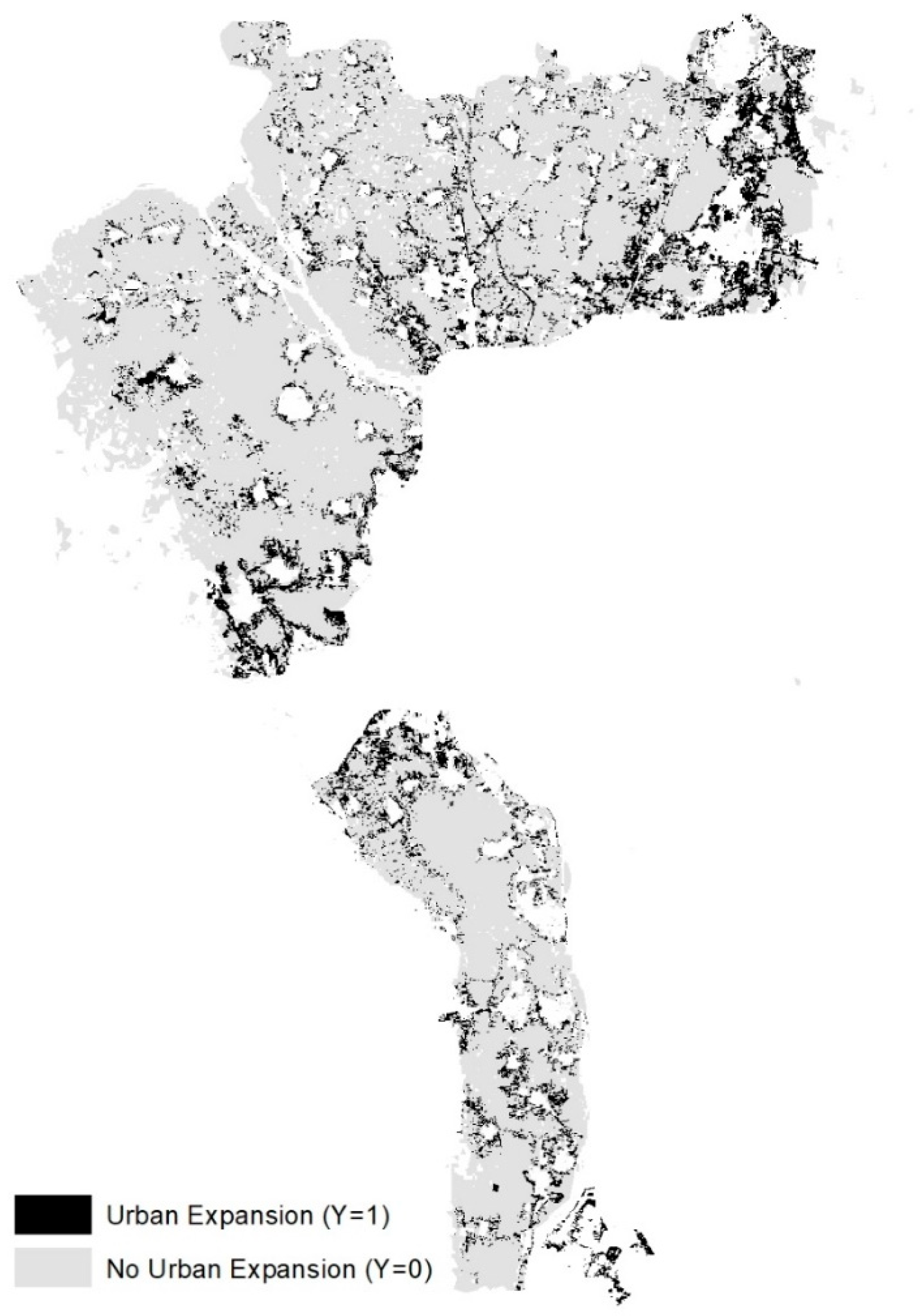
In this model, a map of the urban expansion between 2007 and 2017 was used as a dependent variable to perform the logistic regression analysis. This map has two land use classes: urban expansion (changed cells from agricultural to urban) where y = 1 and no urban expansion (still agricultural land) where y = 0.

Thirteen independent factors (variables) were derived from the literature review and discussion with experts to include in the model [17,19,26,27,36,37]. Then, three factors (income per capita, economic activities and housing rent) were eliminated from the model due to lack of data for the whole study area. In addition, two other factors (distance to Nile River and slope) were eliminated from the model because of the low value of R² statistics with these factors. This process was carried out for each set of variables to assess their reliability. Finally, the total number of independent (variables) decreased from thirteen to eight factors (variables) (see

Table 3. List of factors (variables) included in the logistic regression model.

Variable	Meaning	Nature of Variable
Dependent (Y)	0: no urban expansion; 1: urban expansion	Dichotomous
X1 (dist_Rd)	Distance to nearest road	Continuous
X2 (dist_centrs serv.)	Distance to nearest center of regional services	Continuous
X3 (dist_wtr str.)	Distance to water streams	Continuous
X4 (dist_M.Agg.)	Distance to Main Agglomeration	Continuous
X5 (dist_Indust._Ar)	Distance to Industrial Areas	Continuous
X6 (dist_Urb_centrs)	Distance to nearest urban center	Continuous
X7 (Pop._Density)	Population density	Continuous
X8 (Nmbr_urb_cells3*3)	Number of urban cells within a 3 × 3 cell window	Continuous

).

The number of urban cells within a window was decided according to the most widely used window sizes in dynamic simulation models where sizes are usually 3 × 3, 5 × 5, or 7 × 7 [30,36,38]. Cell windows of 7 × 7, 5 × 5, and 3 × 3 cell windows were investigated during the initial analysis and the best results were found using 3 × 3 cell window. This is probably because the smallest cell could capture the reality of small urban expansion in the study area.

3.3. Logistic Regression Model (LRM)

A logistic regression model was used to analyze the driving factors causing urban expansion in the PUAs of the GCR. The logistic model was utilized to estimate the probability of urban expansion (dependent variable) based on independent variables (X). The dependent variable (Y) in this model is the developed cells (change from non-urban to urban) presented as a binary raster where a value of 1 indicates urban expansion (change on the specific pixels) while 0 indicates no urban expansion (no change on the specific pixels) within the period of 2007–2017.

The analysis was conducted using LOGISTICREG module in Terrset software. The basic assumption is that the probability of the dependent variable taking the value of 1 follows the logistic curve and its value can be calculated with the following Equation (1):

$$\mathrm{P}=(\mathrm{Y}=1|\mathrm{X})=\frac{\exp {{\displaystyle \sum }}_{\mathrm{k}=0}^{\mathrm{k}}{\mathrm{b}}_{\mathrm{k}}{\mathrm{x}}_{\mathrm{i}\mathsf{\kappa }}}{1+\exp {{\displaystyle \sum }}_{\mathrm{k}=0}^{\mathrm{k}}{\mathrm{b}}_{\mathrm{k}}{\mathrm{x}}_{\mathrm{i}\mathsf{\kappa }}}$$

(1)

where P is the probability of the dependent variable being 1; X is the independent variables, x = (x₀, x₁, x₂…x_k) (representing driving factors of urban expansion); and b is the estimated parameters, b = (b₀, b₁, b₂…b_k) (representing variable coefficients)

The state of a cell is dichotomous: either the presence of urban expansion or absence of urban expansion. The logistic regression model employs a Maximum Likelihood Estimation (MLE) procedure to find the best fitting set of coefficients. The maximum likelihood function used by LRM is the following:

$$\mathrm{L}={{\displaystyle \prod }}_{\mathrm{i}=1}^{\mathrm{N}}{\mathsf{\mu }}_{\mathrm{i}}^{{\mathrm{y}}_{\mathrm{i}}}\ast {\left(1-{\mathsf{\mu }}_{\mathrm{i}}\right)}^{\left(1-{\mathrm{y}}_{\mathrm{i}}\right)}$$

(2)

where L is the likelihood; µ_i is the predicted value of the urban expansion (dependent variable) for sample $\mathrm{i}$; and y_i is the observed value of the urban expansion (dependent variable) for sample i.

Maximizing Equation (2) thus requires the solution for the following simultaneous nonlinear equations:

$${{\displaystyle \sum }}_{\mathrm{i}=1}^{\mathrm{N}}\left({\mathrm{y}}_{\mathrm{i}}-{\mathsf{\mu }}_{\mathrm{i}}\right){\ast \mathrm{x}}_{\mathrm{ij}}=0$$

(3)

where X_ij is the observed value of the independent variable j for sample i. The rest is the same as for the likelihood function. In solving the above equations, LOGISTICREG uses the Newton–Raephson algorithm.

In a logistical regression, the odds of Y being 1 is calculated using the equation φ = eα + ∑ βiXi and the odds ratio for the dichotomous variable X is demonstrated as a relation between each of the variables with urban expansion (Y). By fitting the logistic regression model to the variables, the study calculated the respective odds ratios of the independent variables to predict the outcome using Equation (4):

$$\mathrm{P}=\frac{\exp \left(\mathsf{\alpha }+\mathsf{\beta },{\mathrm{X}}_1+{\mathsf{\beta }}_2{\mathrm{X}}_2+\dots +{\mathsf{\beta }}_{\mathrm{n}}{\mathrm{X}}_{\mathrm{n}}\right)}{1+\exp \left(\mathsf{\alpha }+{\mathsf{\beta }}_1{\mathrm{X}}_1+{\mathsf{\beta }}_2{\mathrm{X}}_2+\dots +{\mathsf{\beta }}_{\mathrm{n}}{\mathrm{X}}_{\mathrm{n}}\right)}$$

(4)

where P is the the probability that a case is in a particular category for the response variable; exp = the base of natural logarithms (approximately 2.72); a is the constant of the equation in particularly explicit in step-wise models; and β is the coefficient of the predictor variables.

The study used Terrset software to conduct the LRM using stratified sampling. Sampling can significantly decrease the processing time as well as reduce the negative impact of spatial interdependence [31]. The study used a mask file to select pixels of interest for the analysis as well as apply this mask to the output image.

3.3.1. Calibration of the Logistic Regression Model

The aim of the calibration of the LRM is detecting the ideal resolution for modeling. This study used the same fractal method as Hu and Sefidi to determine the optimal scale of modeling [28,39]. Fractal dimensions were calculated for the probability maps predicted using the LRM calibrated in different resolutions from 30 m to 360 m. Fractal dimension increases almost linearly with the change of resolution from 30 m to 300 m, and then decreases after 300 m. The scale at which the highest fractal dimension is measured might be the scale at which the model performs best [39,40]. To test if the model indeed performs best at the turning point of 300 m, a series of probability maps of urban expansion generated from the LRM was compared against an actual urban growth map and ROC values were calculated (for details of model validation, see Section 4.6). The highest ROC value was achieved at the resolution of 300 m. Therefore, the resolution of 300 m was selected as the scale at which the LRM best represents the dynamics of urban expansion. To reduce the impact of spatial dependency between observations, the study specified a stratified random sampling by taking a 10% portion of total cells. At the resolution of 30 m, the number of cells within the PUA is 4,648,192, of which 444,012 cells have been sampled. The number of cells that have changed from non-urban to urban (Y = 1, urban expansion), is 123,230, accounting for 2.65% of the total number of cells. For the random sample, there are 11,749 points whose cell values are 1 in the Y variable layer. The percentage of urban expansion (Y = 1) in the sample is 2.64%, matching very well with the percentage of 2.65% for the full dataset, which demonstrates the representativeness of the stratified random sampling.

3.3.2. Goodness of Fit of the Model

The −2log(likelihood) was computed to measure the goodness of fit of the logistic regression model. The −2log(likelihood) (1744.354) is the value of the likelihood function for the full model as fitted. Cox and Snell R² and Nagelkerke R² were computed to further test the goodness of fit of the model. The Cox and Snell R² values and the Nagelkerke R² values are analogous indicators to the R² statistics of the linear regression. R² values closer to 1 indicate the model is closer to certainty. The outputs proved that the eight driving factors are significant enough. Cox and Snell R² value for the model was 0.76, which refers to a very good fit in the study area and the R² value was 0.90, which reflects the accuracy of the model (see

Table 4. Goodness-of-fit statistics of the logistic regression in the study area.

Step	−2 Log(Likelihood)	Cox and Snell R2	Nagelkerke R2
1	1744.354	0.76	0.90

).

4. Results

4.1. Urban Expansion

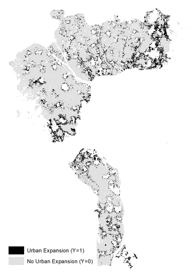
The urban expansion (UE) in the PUAs was about 5400 ha with annual loss of 540 ha. The number of changed cells from agricultural to urban (Y = 1, UE) was 123,230, accounting for 2.65% of the total number of cells as shown in Figure 2. The direction of UE was mainly toward north and northeast area, especially along or near roads network. In addition, there was a significant UE around existing urban areas.

4.2. Driving Factors (Independent Variables)

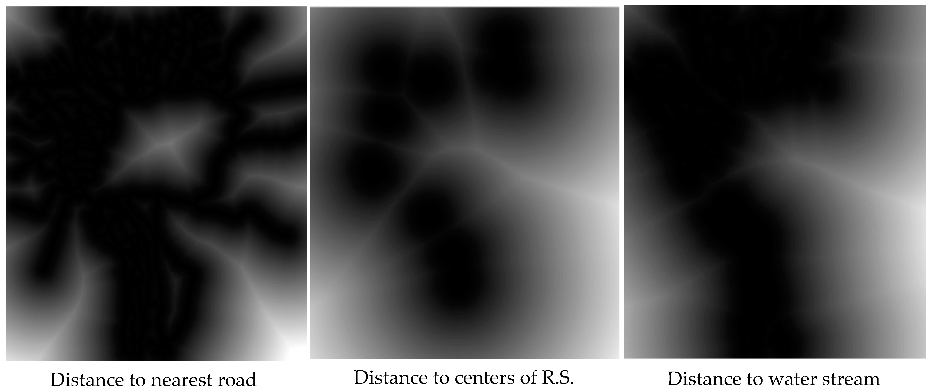
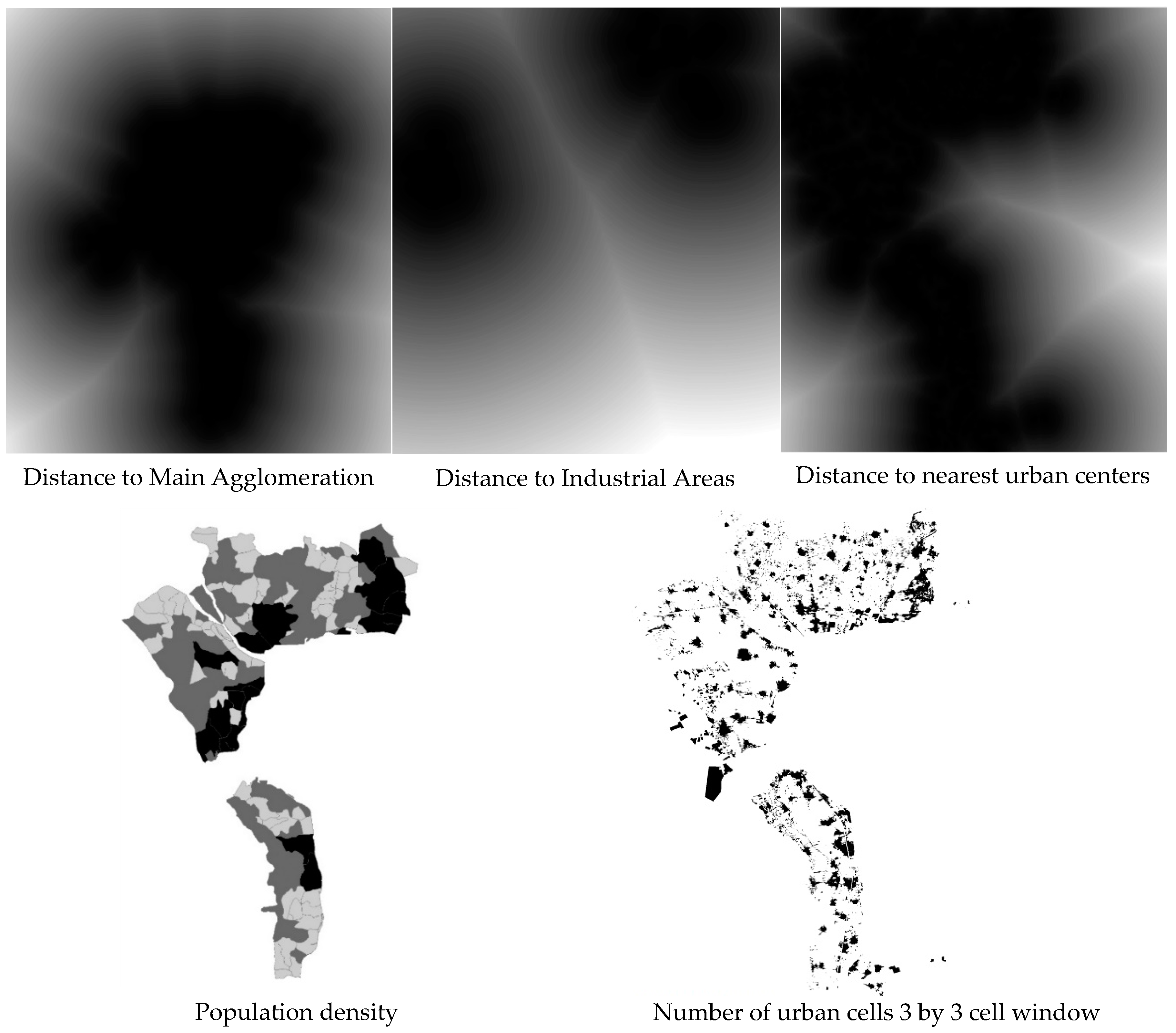
Distance to nearest road, distance to the nearest center of regional services, distance to water streams, distance to the main agglomeration, distance to industrial areas, and distance to nearest urban centers were analyzed in Terrset software using distance command from Idrisi Gis analysis. Number of urban cells within a 3 × 3 cell window was calculated using pattern tool from Context Operators menu in Terrset software (see Figure 3).

4.3. Multicollinearity Analysis for Independent Variables

To eliminate useless driving factors from our model and preserve the reliability of our coefficients, a multicollinearity test was performed for each set of factors in the study area. VIF is the most frequently utilized test to find multicollinearity in statistical analysis. VIF computes how much the variances of the applied regression coefficients are distended compared to when driving factors are not linearly related. The analysis was performed in SPSS by regressing one of the independent variables against the residual seven driving factors in a repeated mechanism. The analysis shows that all driving factors give VIF < 5, which is a good outcome (see

Table 5. Results of multicollinearity analysis.

Model	Collinearity Statistics
	Tolerance	VIF
X1 (dist_Rd)	0.971	1.030
X2 (dist_centrs serv.)	0.620	1.613
X3 (dist_wtr str.)	0.908	1.101
X4 (dist_M.Agg.)	0.572	1.748
X5 (dist_Indust._Ar)	0.759	1.318
X6 (dist_Urb_centrs)	0.905	1.010
X7 (Pop._Density)	0.933	1.072
X8 (Nmbr_urb_cells3*3)	0.978	1.023

).

4.4. Influence of Driving Forces on Urban Expansion

The findings explained the nature of the relationship between urban expansion and the driving factors in the study area. It can be explained that the pixels near any independent variable having higher coefficient value have more development probability for change [18]. The sign of the coefficient (±) indicates a positive or negative correlation to the response of the dependent variable [32]. For example, a negative (−) coefficient index means that, if the distance increased, the urban expansion decreased. The factors of population density (X7) and the number of urban cells within a 3 × 3 cell window (X8) had a positive correlation with urban expansion, while the correlation was negative with the other factors: the distance to nearest road (X1), distance to the nearest center of regional services (X2), distance to water streams (X3), distance to the main agglomeration (X4), distance to industrial areas (X5) and distance to nearest urban centers (X6) (for more details, see

Table 6. Coefficients and odds ratios for the LRM containing the eight independent variables.

Variable	Coefficient	Standard Error	Sig.	Odds Ratio i
X1 (dist_Rd)	−0.114	0.190	0.431	0.861
X2 (dist_centrs serv.)	−0.000	0.000	0.129	1.000
X3 (dist_wtr str.)	−0.000	0.000	0.281	1.000
X4 (dist_M.Agg.)	−0.000	0.000	0.000	1.000
X5 (dist_Indust._Ar)	−0.000	0.000	0.000	1.000
X6 (dist_Urb_centrs)	−0.092	0.130	0.065	1.955
X7 (Pop._Density)	0.540	0.000	0.851	0.110
X8 (Nmbr_urb_cells3*3)	0.096	0.035	0.007	1.909

ⁱ Odds ratio meaning the ratio of the probability of success to the probability of failure for the variable, which represents the effect of each variable in the urban expansion process.

).

The research results show that the eight factors affected the urban expansion to different degrees, as indicated by odds ratios. The odds ratio for distance to the nearest road (X1) is 0.861, which mean that the predicted urban expansion in an area close to a road is estimated as 1.16 times more than the predicted urban expansion in an area 1 km further away from a road. The odds ratio was 1 for distance to nearest center of regional services (X2), distance to water stream (X3), distance to the main agglomeration (X4) and distance to industrial areas (X5), which mean that there is no impact of these factors in the urban expansion process within the study area. The odds ratio of urban expansion probability around existing urban centers (X6) is 1.955, which mean that the odds of urban expansion will decrease by 0.5 if the distance to nearest existing urban area has increased by 1 km. The odds ratio for the population density (X7) is 0.110, which mean that the probabilities of urban expansion in the areas with high density of population are nine times more than the probabilities of urban expansion in the areas with low population density. The odds ratio for the number of urban cells within a neighborhood (measured by a window of 3 × 3 cell size) (X8) is 1.909, which mean that, with an increase of one urban cell within the neighborhood, the probability of urban expansion will increase by 0.5. Therefore, if a land lot includes many urban cells, it is more likely to witness more urban expansion

4.5. Prediction of Urban Expansion

The probability of urban expansion was predicted by using the coefficients of the logistic regression model encompassing the eight variables (driving factors) into the following equation:

$$\mathrm{P}=(\mathrm{Y}=1|{\mathrm{X}}_1,{\mathrm{X}}_2,\dots ,{\mathrm{X}}_{\mathrm{K}})=\frac{1}{1+{\mathrm{e}}^{-\left(\mathsf{\alpha }+{{\displaystyle \sum }}_{\mathrm{i}=1}^{\mathrm{k}}{\mathsf{\beta }}_{\mathrm{i}}{\mathrm{X}}_{\mathrm{i}}\right)}}$$

where P (Y = 1|X₁, X₂, …, X_k) is the probability of the dependent variable Y being 1 given (X₁, X₂, …, X_k), i.e., the probability of a cell being urbanized; Xi is an independent variable representing a driving force of urban expansion; and β_i is the coefficient for variable X_i.

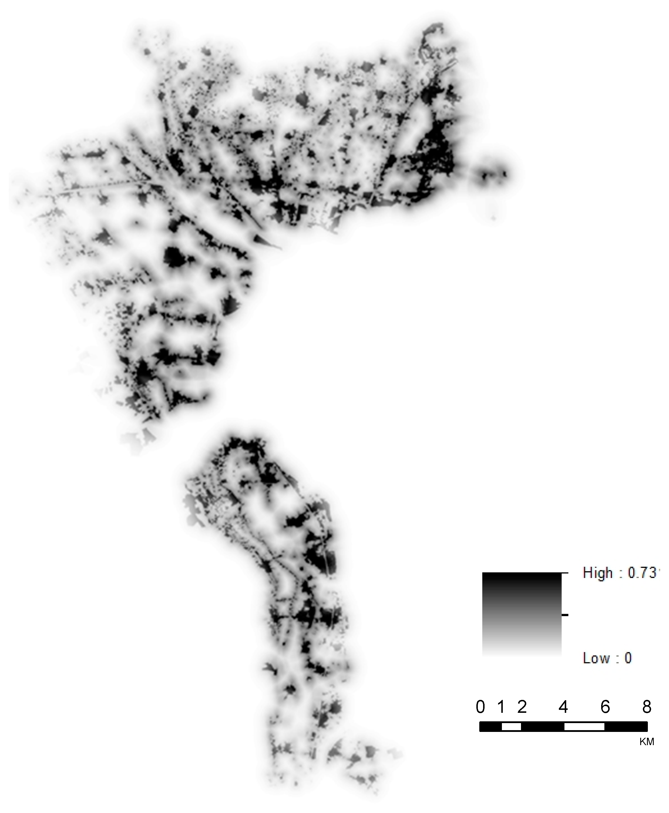
The probability map of urban expansion for the PUAs in Figure 4 is a 0–0.73 color classification of urban expansion probability values. The darker tones indicate higher probabilities of urban expansion. The future pattern of urban expansion is easy to identify from this map, and is expected to be around main existing urban areas and adjacent to roads, particularly in northern areas.

This probability map can be used to predict where urban expansion will happen. Additionally, the study highlighted the major factors of UE, which can be adapted by appropriate policies to promote or discourage UE in the predicted areas.

4.6. Model Validation

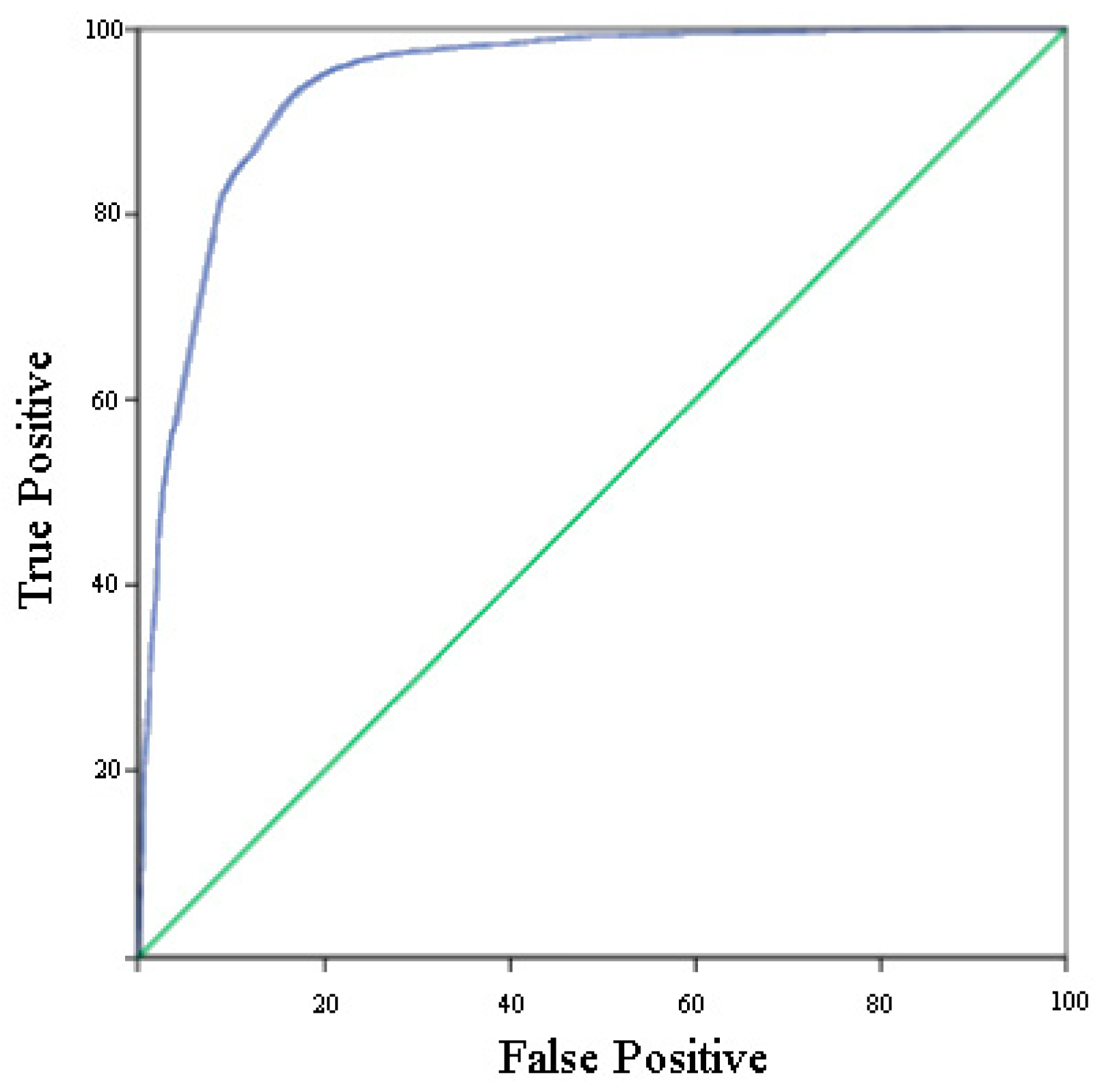
The study used the relative operating characteristic (ROC) curve to examine the efficacy of the model for the probability of urban expansion in the PUA. The ROC computes the area under the curve, which varies between 0.5 and 1.0., where 1 indicates a perfect fit and 0.5 indicates a random fit. The ROC calculates the percentages of false positives and true positives for a range of thresholds or cut-off values, relating them in a chart.

Previous studies show that a perfect spatial agreement can exist between the real urban expansion and the simulated urban expansion by the LRM [34,38,39]. In this study, the model validation was conducted by comparing the predicted urban expansion of the probability map with the actual urban expansion map of 2017 using random samples of 1000 cells in the two maps. The ROC curve is based on several two-by-two contingency tables. The contingency table is based on the comparison between the actual and the predicted probability image.

Table 7. Two by two contingency (the number of grid cells in actual map versus a predicted map).

		Reality (Reference Image)
		Urban Expansion (1)	No Urban Expansion (0)
Predicted Urban Expansion	Urban Expansion (1)	A (true positive)	B (false positive)
	No Urban Expansion (0)	C (false negative)	D (true negative)

shows the contingency table. “A” is the number of true positive cells, which are predicted as urban expansion and agree with the actual image. “B” is the number of false positive cells, which are predicted as urban growth but disagree with the actual image. “C” is the number of false negative cells, which are predicted as non-urban growth but disagree with the actual map. “D” is the number of true negativecells, which are predicted as non-urban growth and agree with the actual image. From every contingency table, a single data point (x, y) is created, where x and y are the rate of false positives and the rate of true positives, respectively.

(True positive %) = A/(A + C)

(False positive %) = B/(B + D)

The true positive percent value is derived from A/(A + C), while the false positive percent value is derived from B/(B + D), where A, B, C, and D are pixel counts in the contingency table for each threshold. The ROC value of the model was 0.93, which indicates that the probability map of urban expansion is valid (see Figure 5).

5. Discussion

Similar to most cities in developing countries, the expected urban expansion in the PUA of GCR will be a kind of chaotic expansion, which probably will establish slums areas on agriculture lands. The findings explain the driving factors that affect the urban expansion in different degrees, which are discussed as follows:

The findings show a lesser effect than expected for the roads factor (distance to nearest road) in comparison with results of similar case studies [27,32,39]. This is probably due to most of the urban expansion occurring on specific regional roads in the study area, and the study investigated all types of roads in the study area. For the neighborhood factor (the number of urban cells within a neighborhood), the findings show a lower effect than common in comparable metropolitan regions [28,39]. However, the expansion will probably continue to take place in locations near developed areas due to the other factors, which will lead to more informal areas.

On the other hand, the findings show that the population density has the greatest effect on urban expansion in the study area and this result is compatible with the findings of most previous studies [25,27]. The findings of this study can be useful to manage expansion in the study area by using appropriate techniques for dealing with the significant driving factors.

The study suggests some recommendations for dealing with urban expansion in the case study and similar areas in the metropolitan regions of developing countries. First, the results obtained from LRM should be used to identify the tendencies of urban expansion in local municipalities. Second, decision makers must recognize and track the rapid population growth in the PUAs and the increasing urban expansion. Accordingly, they should utilize restricted policies to adjust urban expansion on agriculture lands. Third, local urban municipalities in the PUAs should identify the potential growth areas around the high-density urban edges, near roads, and near urban centers, as well as prepare urban plans with strict building regulations to prevent future informal settlements.

Despite the LRM’s potentials in comprising many variables in the analysis, some important factors still cannot be included in the model, for instance government policy factor and real estate speculation factor, which probably influence urban expansion. In addition, the probability map of urban expansion produced by the model indicates where urban expansion will happen without clarification of the temporal dimension. Therefore, it is recommended for future research to integrate Cellular Automata (CA) model with the logistic regression model to predict urban expansion. Finally, the study suggests a separate research on the mechanisms of land management in PUAs, especially for the lands situated along major roads.

6. Conclusions

This study identified eight driving factors causing the urban expansion within the PUAs in the GCR, and then analyzed their influence on the urban expansion process using LRM. The population density and distance to the nearest road were the most significant driving factors in the study area during the last 10 years (2007–2017). Moreover, the probability map generated from the model can be used to predict where urban expansion will occur. The ROC value was used to examine the efficacy of the model for the probability of urban expansion, which indicated that the model is valid. Despite the LRM’s strengths, this study has shown some limitations of the model, most notably the inability to include all types of variables.

On the other hand, the results of this study are not only useful to manage UE in the study area, but also in other PUA in developing countries. The study identified the major factors of urban expansion, which can be controlled by using the appropriate regulations and policies.

The study suggests combining Cellular Automata (CA) model with LRM to overcome the weakness of LRM in dealing with temporal dynamics. In addition, the future research should address the role of government policies and real estate speculation in the urban expansion process in the GCR. Moreover, the study suggests more future research on the mechanisms of land management in PUAs, especially for lands situated along major roads.

References

1. Bhatta, B. Remote Sensing, GIS, and Urban Analysis. In Analysis of Urban Growth and Sprawl from Remote Sensing; Springer: Berlin/Heidelberg, Germany, 2010; pp. 49–63. [Google Scholar] [CrossRef]
2. Dutta, V. Land Use Dynamics and Peri-Urban Growth Characteristics: Reflections on Master Plan and Urban Suitability from a Sprawling North Indian City. Environ. Urban. Asia 2012, 3, 277–301. [Google Scholar] [CrossRef]
3. Ramachandra, T.V.; Bharath, A.H.; Sowmyashree, M.V. Monitoring Urbanization and Its Implications in a Mega City from Space: Spatiotemporal Patterns and Its Indicators. J. Environ. Manag. 2015, 148, 67–81. [Google Scholar] [CrossRef] [PubMed]
4. McGregor, D.; Simon, D.; Thompson, D. The Peri-Urban Interface: Approaches to Sustainable Natural and Human Resource Use; Earthscan: London, UK, 2012. [Google Scholar] [CrossRef]
5. Das, N.D. Land-Use Dynamics of Peri-Urban Areas of Metropolitan Cities with Special Focus on Delhi. In Marginalization in Globalizing Delhi: Issues of Land, Livelihoods and Health; No. Issues of Land, Livelihoods and Health; Springer: New Delhi, India, 2017; pp. 21–42. [Google Scholar] [CrossRef]
6. Chirisa, I.; Mazhindu, E.; Bandauko, E. Peri-Urban Developments and Processes in Africa with Special Reference to Zimbabwe; Springer International Publishing: Basel, Switzerland, 2016. [Google Scholar] [CrossRef]
7. Allen, A. Environmental Planning and Management of the Peri-Urban Interface: Perspectives on an Emerging Field. Environ. Urban. 2003, 15, 135–148. [Google Scholar] [CrossRef]
8. Dupont, V.E.; Centre, D.S.H. Peri—Urban Dynamics: Population, Habitat and Environment on the Peripheries of Large Indian Metropolises. In Population (English Edition); CSH: New Delhi, India, 2006; pp. 1–151. [Google Scholar] [CrossRef]
9. Webster, D.; Muller, L. Peri-Urbanization: Zones of Rural-Urban Transition. In Human Settlement Development Volume 1; Sassen, S., Ed.; EOLSS Publications: Paris, France, 2009; Volume 1, pp. 281–290. [Google Scholar]
10. Salem, M. Peri-Urban Dynamics and Land-Use Planning for the Greater Cairo Region in Egypt. In WIT Transactions on The Built Environment; WIT Press: Southampton, UK, 2015; Volume 168, pp. 109–119. [Google Scholar] [CrossRef]
11. Sarkar, S.; Bandyopadhyay, S. Dynamics of the Peri Urban Interface: Issues and Perspectives for Management. Trans. Inst. Indian Geogr. 2013, 35, 49–62. [Google Scholar]
12. Iaquinta, D.L.; Drescher, A.W. Defining the Peri-Urban: Rural-Urban Linkages and Institutional Connections. Land Reform 2000, 2, 8–26. [Google Scholar]
13. Miljković, J.Ž.; Crnčević, T.; Marić, I. Land Use Planning for Sustainable Development of Peri-Urban Zones. Spatium 2012, 28, 15–22. [Google Scholar] [CrossRef]
14. Aguilar, A.G. Peri-Urbanization, Illegal Settlements and Environmental Impact in Mexico City. Cities 2008, 25, 133–145. [Google Scholar] [CrossRef]
15. Fish, B.; Phelan, K.; Buxton, M.; Farrell, S. Peri-Urban Futures: Scenarios for Sustainable Regional Development Report; RMIT University: Melbourne, Australia, 2014. [Google Scholar]
16. Bhatta, B. Causes and Consequences of Urban Growth and Sprawl. In Analysis of Urban Growth and Sprawl from Remote Sensing Data; Springer: Berlin/Heidelberg, Germany, 2010; pp. 17–37. [Google Scholar] [CrossRef]
17. Ju, H.; Zhang, Z.; Zuo, L.; Wang, J.; Zhang, S.; Wang, X.; Zhao, X. Driving Forces and Their Interactions of Built-up Land Expansion Based on the Geographical Detector—A Case Study of Beijing, China. Int. J. Geogr. Inf. Sci. 2016, 30, 2188–2207. [Google Scholar] [CrossRef]
18. Siddiqui, A.; Siddiqui, A.; Maithani, S.; Jha, A.K.; Kumar, P.; Srivastav, S.K. Urban Growth Dynamics of an Indian Metropolitan Using CA Markov and Logistic Regression. Egypt. J. Remote Sens. Space Sci. 2018, 21, 229–236. [Google Scholar] [CrossRef]
19. Osman, T.; Divigalpitiya, P.; Arima, T. Driving Factors of Urban Sprawl in Giza Governorate of the Greater Cairo Metropolitan Region Using a Logistic Regression Model. Int. J. Urban Sci. 2016, 20, 206–225. [Google Scholar] [CrossRef]
20. Lawanson, T.; Yadua, O.; Salako, I. An Investigation of Rural-Urban Linkages of The Lagos Megacity, Nigeria. J. Constr. Proj. Manag. Innov. 2012, 2, 464–481. [Google Scholar]
21. Braimoh, A.K.; Onishi, T. Spatial Determinants of Urban Land Use Change in Lagos, Nigeria. Land Use Policy 2007, 24, 502–515. [Google Scholar] [CrossRef]
22. Appiah, D.O.; Bugri, J.T.; Forkuor, E.K.; Boateng, P.K. Determinants of Peri-Urbanization and Land Use Change Patterns in Peri-Urban Ghana. J. Sustain. Dev. 2014, 7, 95–109. [Google Scholar] [CrossRef]
23. Mahamud, M.A.; Samat, N.; Mohd Noor, N. Identifying Factors Influencing Urban Spatial Growth for The George Town Conurbation. Plan. Malays. J. 2016, 14. [Google Scholar] [CrossRef]
24. Jokar Arsanjani, J.; Helbich, M.; Kainz, W.; Darvishi Boloorani, A. Integration of Logistic Regression, Markov Chain and Cellular Automata Models to Simulate Urban Expansion. Int. J. Appl. Earth Obs. Geoinf. 2013, 21, 265–275. [Google Scholar] [CrossRef]
25. Mohamed, H.E. Analysis of Urban Growth at Cairo, Egypt Using Remote Sensing and GIS. Nat. Sci. 2012, 4, 355–361. [Google Scholar] [CrossRef]
26. Sims, D. Understanding Cairo: The Logic of a City Out of Control; The American University in Cairo Press: Cairo, Egypt, 2011. [Google Scholar] [CrossRef]
27. Salem, M.; Tsurusaki, N.; Divigalpitiya, P.; Osman, T. Driving Factors of Urban Expansion in Peri-Urban Areas of Greater Cairo Region. In REAL CORP 2018–EXPANDING CITIES–DIMINISHING SPACE. Are “Smart Cities” the Solution or Part of the Problem of Continuous Urbanisation Around the Globe? Proceedings of 23rd International Conference on Urban Planning, Regional Development and Information, Vienna, Austria, 4–6 April 2018; REAL CORP: Vienna, Austria, 2018; pp. 191–196. [Google Scholar]
28. Sefidi, A.K.B.; Ghalehnoee, M. Analysis of Urban Growth Pattern Using Logistic Regression Modeling, Spatial Autocorrelation and Fractal Analysis Case Study: Ahvaz City; Iran University of Science & Technology: Tehran, Iran, 2016; Volume 26, pp. 183–194. [Google Scholar] [CrossRef]
29. Poelmans, L.; Van Rompaey, A. Complexity and Performance of Urban Expansion Models. Comput. Environ. Urban Syst. 2010, 34, 17–27. [Google Scholar] [CrossRef]
30. Hamdy, O.; Zhao, S.; Osman, T.; Salheen, M.; Eid, Y. Applying a Hybrid Model of Markov Chain and Logistic Regression to Identify Future Urban Sprawl in Abouelreesh, Aswan: A Case Study. Geosciences 2016, 6, 43. [Google Scholar] [CrossRef]
31. Tobergte, D.R.; Curtis, S. Logistic Regression, A Self-Learning Text; Springer Science & Business Media: Berlin, Germany, 2013; Volume 53. [Google Scholar] [CrossRef]
32. Clark, W.A.V.; Hosking, P.L. Statistical Methods for Geographers; Wiley: Hoboken, NJ, USA, 1986. [Google Scholar]
33. Nong, Y.; Du, Q. Urban Growth Pattern Modeling Using Logistic Regression. Geo-Spat. Inf. Sci. 2011, 14, 62–67. [Google Scholar] [CrossRef]
34. Liao, F.H.F.; Wei, Y.H.D. Modeling Determinants of Urban Growth in Dongguan, China: A Spatial Logistic Approach. Stoch. Environ. Res. Risk Assess. 2014, 28, 801–816. [Google Scholar] [CrossRef]
35. Japan International Cooperation Agency (JICA). The Strategic Urban Development Master Plan (SDMP) Study For Sustainable Development Of The Greater Cairo Region; Japan International Cooperation Agency: Tokyo, Japan, 2008; Volume 1.
36. Shu, B.; Zhang, H.; Li, Y.; Qu, Y.; Chen, L. Spatiotemporal Variation Analysis of Driving Forces of Urban Land Spatial Expansion Using Logistic Regression: A Case Study of Port Towns in Taicang City, China. Habitat Int. 2014, 43, 181–190. [Google Scholar] [CrossRef]
37. Chen, L.; Ren, C.; Zhang, B.; Wang, Z.; Liu, M. Quantifying Urban Land Sprawl and Its Driving Forces in Northeast China from 1990 to 2015. Sustainbility 2018, 10, 188. [Google Scholar] [CrossRef]
38. Huang, Q.H.; Cai, Y.L.; Peng, J. Modeling the Spatial Pattern of Farmland Using GIS and Multiple Logistic Regression: A Case Study of Maotiao River Basin, Guizhou Province, China. Environ. Model. Assess. 2007, 12, 55–61. [Google Scholar] [CrossRef]
39. Hu, Z.; Lo, C.P. Modeling Urban Growth in Atlanta Using Logistic Regression. Comput. Environ. Urban Syst. 2007, 31, 667–688. [Google Scholar] [CrossRef]
40. Lam, N.S.N.; Quattrochi, D. On the Issues of Scale, Resolution, and Fractal Analysis in the Mapping Sciences. Prof. Geogr. 1992, 44, 88–98. [Google Scholar] [CrossRef]
Figure 1. Study area.
Infrastructures 04 00004 g001
Figure 2. Dependent variable (Y): the change to urban area from 2007 to 2017.
Infrastructures 04 00004 g002
Figure 3. Raster layers of independent variables.
Infrastructures 04 00004 g003aInfrastructures 04 00004 g003b
Figure 4. Probability map of urban expansion in the PUAs.
Infrastructures 04 00004 g004
Figure 5. Relative operating characteristics (ROC) curve.
Infrastructures 04 00004 g005