Resilience-Based Recovery Assessments of Networked Infrastructure Systems under Localized Attacks

Abstract

To reduce unforeseen disaster risks, infrastructure systems are expected to be resilient. The impact of many natural disasters on networked infrastructures is often observed to follow a localized attack pattern. The localized attack can be demonstrated by the failures of a group of links concentrated in a particular geographical domain which result in adjacent isolated nodes. In this paper, a resilience-based recovery assessment framework is proposed. The framework aims to find the most effective recovery strategy when subjected to localized attacks. The proposed framework was implemented in a lattice network structure inspired by a water distribution network case study. Three different recovery strategies were studied with cost and time constraints incorporated: preferential recovery based on nodal weight (PRNW), periphery recovery (PR), and localized recovery (LR). The case study results indicated that LR could be selected as the most resilient and cost-effective recovery strategy. This paper hopes to aid in the decision-making process by providing a strategic baseline for finding an optimized recovery strategy for localized attack scenarios.

1. Introduction

Resilience is known to be one of the most important metrics for measuring the capability of an infrastructure system to cope with changes. It is the ability of a system to withstand an unusual event that might cause damage to the system and recover efficiently from such damage immediately [1,2]. The proper functioning of our society depends highly on several critical infrastructure systems, including power systems, transportation networks, water supply, internet and communication, and others. The interdependency and complexity between various infrastructure systems are growing simultaneously with the global vision to achieve smarter and more connected societies and/or communities [3]. However, this interdependency between infrastructures is one of the main reasons behind the vulnerability of the system towards unexpected failures and disruptions. Besides, the occurrence of unexpected natural disasters can also disrupt the normal operating conditions of infrastructure systems. In networked infrastructure systems, natural disasters are often modeled as localized attacks which cause failures of aggregated components in a geographical domain [4]. It is essential for any infrastructure systems to possess a disaster resilient property. To survive localized attacks and withstand possible failures, infrastructure systems should be recovered within the shortest possible time. Thus, the implemented recovery strategies should ensure the efficiency and robustness during recovery under a certain set of constraints, for example, time, cost, and other resources constraints.

Resilience is a multidimensional concept that can be described from different perspectives. In infrastructure systems, resilience could be defined as the ability of a system to be prepared for any disruptions, absorb and adapt to such disturbances, and recover from them immediately after the disruption [5,6]. The resilience of infrastructure systems is also associated with the ability of the system to maintain a certain level of service even after the occurrence of an extreme event and regain its functionality immediately. In fact, resilience can be defined more appropriately by four dimensions: robustness (the ability to withstand extreme events and deliver a certain level of service after the occurrence of disruptive events), rapidity (the speed of recovering from a disaster), redundancy (the substitutable components within the system), and resourcefulness (the availability of resources to respond to a disaster) [1]. Although reliability is an important aspect of system resilience, a traditional reliability assessment alone may not be adequate [7]. Thus, while describing resilience, reliability is often paired with recoverability [8,9,10]. Reliability is emphasized more on dependability, which is the ability of a system to function normally under certain conditions during a specified operational time, while recoverability is the ability of the system to recover after a failure occurred [11]. System reliability and recoverability complement each other and are highly related to the resilience of a system. To maintain the desired level of system performance in the presence of disruptive events, an assessment of infrastructure resilience must be conducted [12,13].

To quantify infrastructure resilience, several resilience metrics have been developed and implemented in a wide range of cases studies for example, from supply networks [14,15,16], urban systems [17,18,19], to transportation infrastructures [4,20,21]. The quantification of the resilience property for infrastructures application is directly connected to the functionality of the networks. Bocchini et al. proposed the usage of resilience triangle to explain the loss of resilience due to an extreme event and how the recovered functionality can improve the system resilience [1]. Mattsson and Jenelius conducted a study on the role of vulnerability analysis in strengthening system resilience in infrastructure networked systems [2]. Adams et al. proposed two measures of resilience—reduction and recovery—and quantified them with the resilience triangle formulation [6]. Cox et al. presented operational metrics from the perspective of economic resilience and explained the relationship of the system resilience based on the economic aspect [13]. Murray-Tuite measured transportation resilience through four dimensions: adaptability, safety, mobility, and recovery [20]. Future planning is known to play an important aspect in postdisaster infrastructure recovery. Zorn and Shamseldin compared recovery strategies with different disaster types to produce restoration rates for future disasters [22]. To compliment an effective future planning, several resilience-based optimization models were also developed. Liao et al. formulated an optimization model for the resilience of transportation networks under budget and time constraints [23]. The formulated model was implemented on a transportation network under disaster. A bilevel facility protection model was developed by Losada et al. for optimizing system resilience [24]. Turnquest and Vugrin introduced a stochastic optimization model for designing infrastructure network resilience [25]. The importance of restoration in achieving disaster resilient was addressed several times. For the optimization of restoration policies for electric power distribution systems under extreme weather condition, a modeling framework was proposed in Ref. [26]. A resilience-based model was also designed for a supply chain network by Margolis et al. [27]. Another most recent contribution to developing a resilience-driven restoration model was made by Almoghathawi et al. [28]. While planning for postdisaster restoration, considering several uncertainties is crucial. Fang and Sansavini investigated the effects of uncertain repair time and resources on postdisaster restoration. They proposed a two-stage optimization model to solve this problem [29].

From the aforementioned studies it is observed that there exists a wide variety of resilience metrics in measuring infrastructure resilience and optimization models to improve resilience. Resilience is always related to “bouncing-back” properties, in which infrastructure systems are commonly related to postdisaster recovery or restoration strategies. There are many approaches to recovering an infrastructure from failures. However, in order to ensure that a targeted resilience level is attainable, these recovery strategies should be assessed based on the impacts of each strategy on the overall system’s resilience. Thus, in this paper a fundamental resilience-based recovery assessment is proposed for infrastructure networks under localized attacks. The assessment of recovery is considered as resilience-based because the effectiveness of potential recovery strategies is compared based on their resilience value. It should be noted that the modeling details are not covered in detail in this paper. For further references, interested readers are encouraged to review some of the related works that complement this paper such as modeling spatially localized attack and identifying critical locations [30], integrated dynamical modeling for infrastructure resilience [31], and operational models for infrastructure resilience [32,33,34]. Although there has been some related work regarding quantifying or assessing resilience in infrastructure systems, the contribution of this paper is the assessment of the recovery strategies that will eventually lead to improving infrastructure resilience. The proposed approach is different from the traditional ways of evaluating recovery, such as those based on cost, time, and resources utilized. In addition, this paper will focus only on localized attack scenarios, where the effects of the damaged network are portrayed as a set of isolated nodes. To demonstrate the proposed approach, three recovery strategies that were known to be effective in recovering the damages induced by a localized attack were assessed on the basis of the overall system resilience. These recovery strategies are periphery recovery (PR), preferential recovery based on nodal weight (PRNW), and localized recovery (LR). In order to recover a system, there will always be additional resources required. A multiobjective optimization model considering the required recovery cost and time for each recovery strategy is also developed as a part of the overall framework. The proposed approach is a fundamental assessment, in other words, it is a basic and generalized assessment approach that can be modified to fit various applications of interests.

The rest of this paper is organized as follows. Section 2 elaborates on localized attacks, the three recovery strategies, and the proposed resilience-based recovery assessment. Section 3 discusses the resilience metric and the optimization model used for quantifying infrastructure resilience. In Section 4, the recovery assessment of a water distribution network is presented using the proposed framework and optimization model. Finally, conclusions and future work are presented in Section 5. This preliminary research aims to find an effective way to compare multiple recovery strategies for infrastructure protections against various possible attacks and failures.

2. Recovery Strategies against Localized Attacks

In this section, a general scenario of localized attacks in infrastructure networks and three recovery strategies that are known to be effective against localized attacks will be discussed in detail. A resilience-based recovery assessment framework to compare the recovery strategies on the basis of system resilience will also be presented in this section.

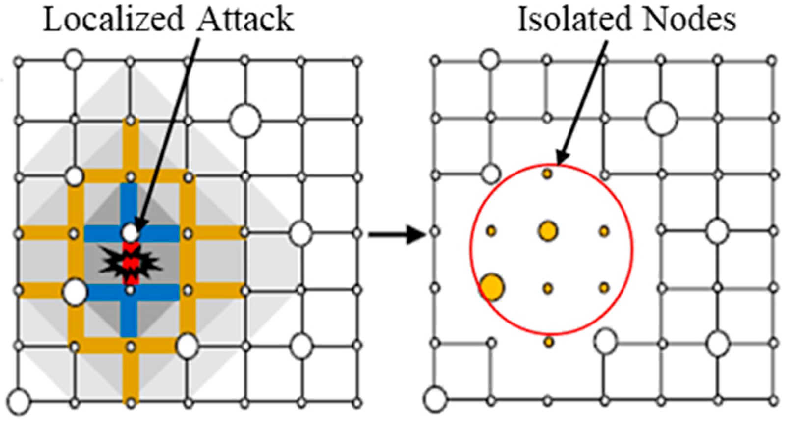
2.1. Localized Attacks

Localized attacks are one of the most common attacks that occur geographically in specific areas. These attacks can be induced by the occurrence of natural disasters, internal critical components failures, or mass/multiple attacks in a specific location [3]. The localized attack in infrastructure networks can be demonstrated by the failure of a group of links concentrated in a particular geographical domain which results in adjacent isolated nodes. Localized attacks could be one of the main reasons behind the aggregated destruction of adjacent components. This kind of attacks might have a devastating impact on the performance and structure of the network. The failure mechanism of localized attack is illustrated in Figure 1. The disruptive event in the case study (presented in the later sections) is modeled to follow localized attacks.

2.2. Recovery Strategies

Various recovery strategies have been proposed to deal with different kind of attacks or failures. In this paper, only three recovery strategies for the localized attack will be presented. In order to recover a system faster after the occurrence of a disruptive event, a proper recovery strategy should take into account the recovery order, allocated time and resources, and other network properties. Many researchers have worked in this area and developed several recovery strategies for localized attacks. Hu et al. proposed PR and PRNW [3] and Shang proposed the LR method [35]. Please note that the recovery strategies against localized attacks are not limited to only the three strategies presented in this paper. The three strategies are illustrated in Figure 2. When localized attacks occur, a group of localized edges failed and were removed from the network. In Figure 2A the edges colored red, blue, and yellow are the affected edges. Consequently, the nodes connected through those edges become isolated, as shown in Figure 2B. The three recovery strategies for localized attack can be summarized as:

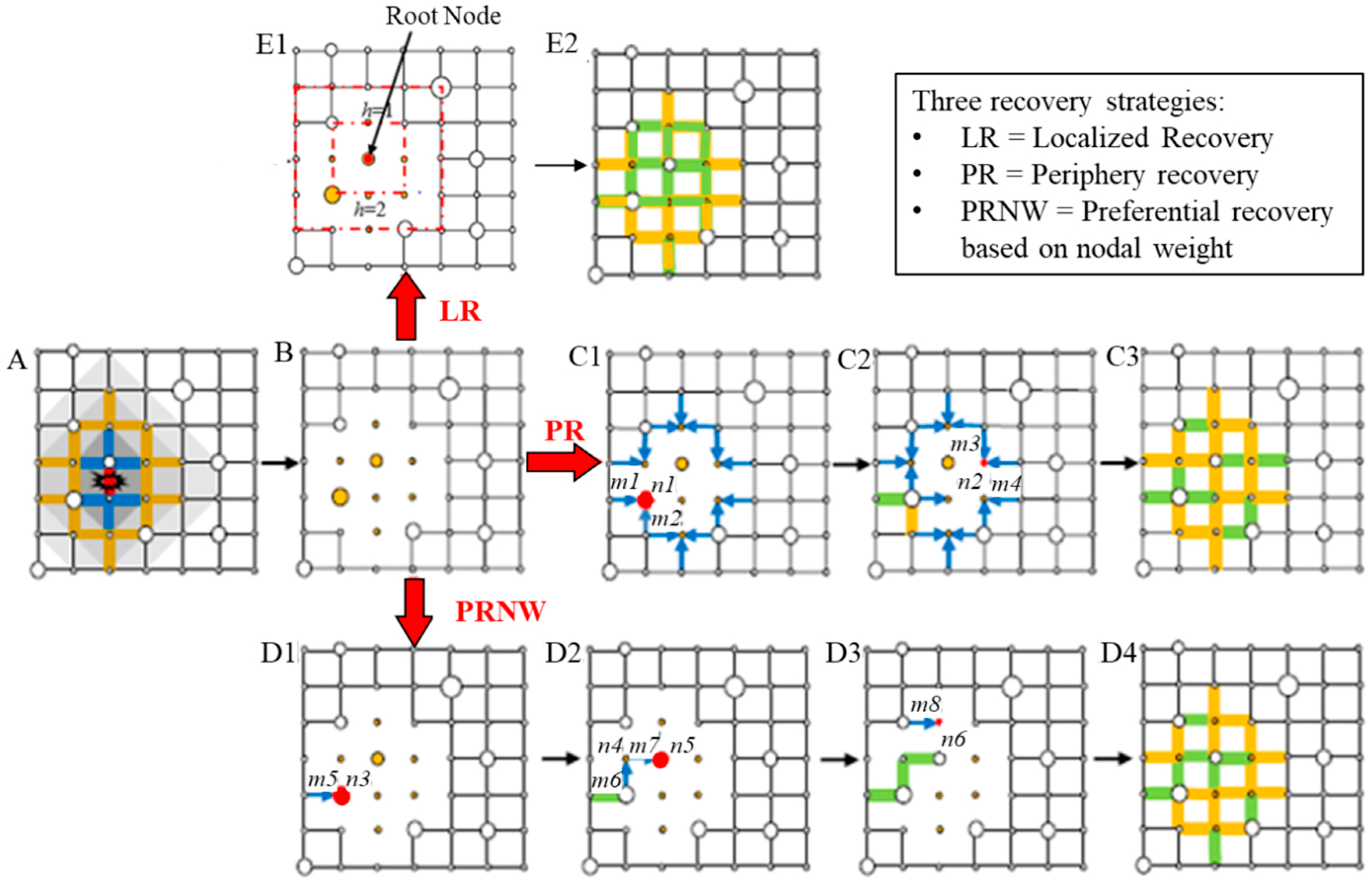
• Periphery recovery (PR). Recovery priorities are given to the most populated isolated node at the boundary [4]. In Figure 2(C1), the blue edges with arrowheads are the damaged edges adjacent to the functional components of the network. The red node n1 is the most populated boundary node of the functional network. According to this recovery rule, either edges m1 or m2 would be repaired first randomly. In this case, m1 is selected to be restored first and colored green. After all the isolated nodes are connected, m2 is repaired and colored yellow. At the next step, the node n2, in Figure 2(C2), is the most populated boundary node of the functional network, and either edge m3 or edge m4 is supposed to be repaired randomly. The process would be iterated until all the isolated nodes were connected to the functional network, as shown in Figure 2(C3). At last, the yellow edges are repaired randomly one by one until all are repaired.
• Preferential recovery based on nodal weight (PRNW). In this method, the repair preference is given to the links that could connect the most populated isolated nodes to the functional component of the network [4]. In Figure 2(D1), the red node n3 has the largest population among all the isolated nodes, and edge m5 connects edge n3 to the network. According to the PRNW algorithm, edge m5 is repaired first and colored green. Following the same procedure, the most populated node—n5—is connected to the functional network through the edges m6 and m7 in Figure 2(D2) and m8 in Figure 2(D3). The steps are iterated until all the isolated nodes are connected to the network, as shown in Figure 2(D4). At last, the yellow edges are repaired randomly one by one until all edges are repaired. PRNW shows high efficiency in connecting the most populated area reducing the recovery time. It can also provide a rational solution while limited resources are available.
• Localized recovery (LR). A localized recovery is where the priority of being recovered is given to the edges of a root node as well as its neighboring nodes, respectively [35]. This recovery process begins with the selection of root nodes. The rest of the nodes are listed in order of their distance from the root node as shown in Figure 2(E1). Nodes being in the same distance from the root node are placed in the same shell. The edges of the root node are recovered first with the edges connected to it. Then the nodes in the same shell h are randomly selected and their edges are further recovered. After all the nodes in the first shell h = 1 are recovered, recovery in the next shell h + 1 starts. The recovery process stops when all the edges are recovered, as shown in Figure 2(E2).

2.3. Resilience-Based Recovery Assessments Framework

For the resilience assessment of an infrastructure system, assessing the recovery strategies with the aim of achieving the highest resilience is crucial. A fundamental resilience-based assessment framework to evaluate and compare various recovery methods is proposed as shown in Figure 3. The assessment of recovery starts by defining the failure characteristics and the causes behind that failure. This step takes into account the types of attack as well as the failure patterns. Different types of attack (localized, malicious, random, etc.) may result in various patterns (random, targeted, cascading, secondary, etc.). The scope of this paper is limited to localized attacks with random failure patterns. However, a critical infrastructure system can suffer from other combinations of attacks and failure patterns.

A comparison among the recovery methods can be performed by building a comparison matrix. The next step is to find the goal of recovering the network. For examples, the objective function can be set to maximize the network resilience or to minimize the recovery time, or the combination of both. While recovering a damaged network, many constraints might exist, for example, network properties, recovery priorities, available resources, cost, time limitation, etc. Taking these factors into account during the assessment is necessary as the recovery process is highly affected by them. One of the most important steps in developing the comparison matrix is to quantify the system resilience after implementing each recovery strategy. Many resilience metrics were developed to quantify infrastructure resilience from various concepts and point of views [11,36]. However, there has not yet been any standard or framework for choosing the most efficient and robust recovery strategy to be implemented based on resilience value. This could be due to confusion on how resilience should be measured. The decision-makers should decide on one resilience metric to measure infrastructure resilience. Thus, each recovery strategy can be compared with the same metric.

During the recovery process, there are some important factors that must be considered, such as the recovery priorities, budget, allowable time, and available resources. With the presence of all these constraints, multiple objective functions could be formulated and solved accordingly. For example, if achieving the highest system resilience is the main aim of an optimum recovery strategy, it can be achieved with the combination of maximizing performance, minimizing recovery time, and minimizing loss. A recovery strategy can be deemed effective when it can be implemented successfully with all the present constraints, while, at the same time, achieving a maximum possible resilience level.

Optimality and feasibility analyses are important while evaluating a recovery process and should be taken more seriously prior to the implementation stage. A recovery method could accelerate the recovery process with a high cost and enormous resources. However, in many cases, these resources and costs may be limited and not constantly available at their times of need. On the other hand, a recovery process could be implemented at low-cost with minimum resources, however typically it can be time-consuming. This could lead to a multiobjective optimization problem with cost, resource, and time constraints. By solving this problem, it is possible to find an optimum recovery strategy. After performing the optimality and feasibility analysis, the desired network recovery strategy can be selected for implementation. The results found from the implementation of the selected recovery strategy might provide an insight into the improvement as well as developing a better strategy. These resulting factors include restoration sequence, number of iterations, resilience value, etc. From these values, the trade-offs between these attributes can be understood and the scopes of improvement can be discovered. This information should be saved and used towards continuous improvement efforts of the resilience-based recovery assessment with the assistance of adaptive learning methodologies.

3. Infrastructure Resilience

Infrastructure resilience can be defined as the ability of the system to maintain or restore its service level even after a disturbance [6]. In other words, resilience is a characteristic that represents system performance under unusual conditions, recovery speed, and required actions for recovery to its original functional state [22]. It is a component importance measure related to system reliability and recovery after an attack or failure [12,19]. According to C. Whitson et al., resilience is a composite of (1) the ability of an infrastructure system to provide service despite external failures and (2) the time to restore service when in the presence of such failures [10]. Ouyang et al. defined resilience of an infrastructure system as its joint ability to resist, prevent, and withstand any possible hazards; absorb the initial damage; and recover to normal operation [9]. Bruneau et al. described resilience as a comprehensive concept of aspects that are listed in Figure 4, which is the combination of four dimensions (technical, organizational, social, and economic), four properties (robustness, rapidity, redundancy, and resourcefulness), and three outcomes (higher reliability, lower consequences, and faster recovery) [1,36].

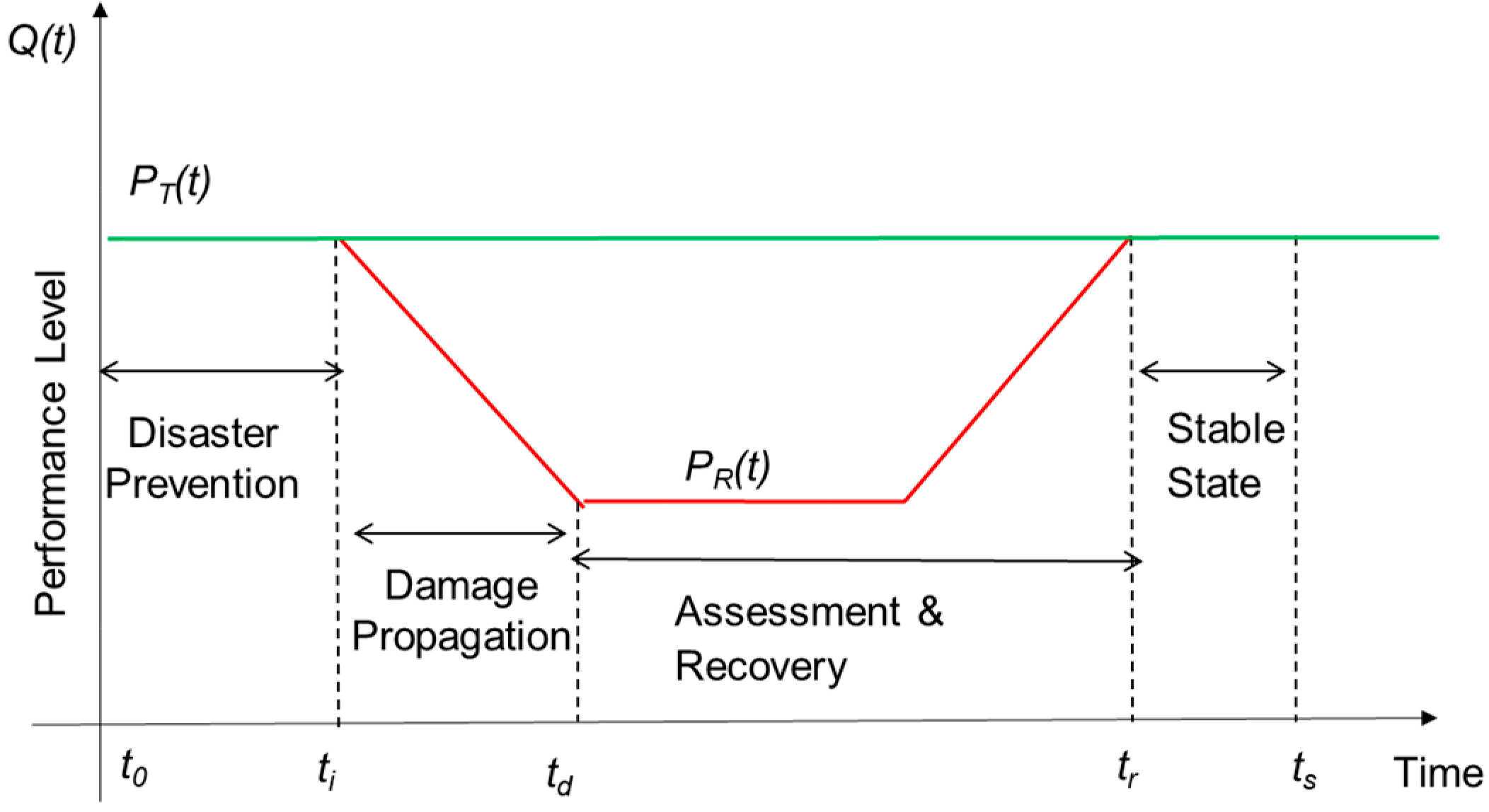
3.1. Resilience Metric

Quantification of infrastructure resilience has gained a lot of attention from different communities such as researchers, engineers, practitioners, and policy-makers. Several resilience metrics have been developed from a variety of aspects in the past years [11]. Robustness, recoverability, adaptability, and reliability are some examples of the important aspects of a resilience metric. As each metric is built upon one or more of these aspects, it is more likely to result in resilience measure that varies in values and scales. This is one of the major challenges for practitioners when it comes to selecting the most appropriate metrics for quantifying infrastructure resilience. In this paper, the resilience metric employed follows the resilience metric proposed by Ouyang et al. According to them, the resilience assessment framework for most networked systems can be divided into various stages: (1) a disaster prevention stage (t₀ ≤ t ≤ t_i), (2) a damage propagation stage (t_i ≤ t ≤ t_i), (3) an assessment and recovery stage (t_d ≤ t ≤ t_r), and (4) a stable state after the recovery process is fully completed (t_r ≤ t ≤ T), as shown in Figure 5 [9]. From this framework, resilience value can be quantified according to the targeted performance curve P_T(t) and the real performance curve P_R(t) as

$$\mathsf{\Phi }\left(t\right)=\frac{{\int }_{t_0}^T{P}_R\left(t\right)dt}{{\int }_{t_0}^T{P}_T\left(t\right)dt}$$

(1)

3.2. Resilience Optimization

Finding a resilience-based optimum recovery strategy has been a matter of great challenge for decision-makers. Researchers have been working on this field in recent years. Liao et al. proposed a transportation resilience optimization model considering recovery activities [23]. A stochastic optimization model was introduced by Turnquist and Vugrin for network resilience, where postdisaster recovery was combined with investments [25]. For the evaluation of restoration policies, a resilience-based optimization model was formulated by Figqueroa-Candia et al. [26]. A resilience-driven restoration model was also proposed for interdependent infrastructure networks [28]. From these references, it is obvious that the existence of a huge variety of constraints, such as resources, cost, and time during the recovery process, could be the reason behind the complexity of the optimization process. This encourages the formulation of a multiobjective optimization problem. A general multiobjective optimization for selecting a recovery strategy among the existing recovery strategies is formulated in this subsection. The main goal of this assessment model is to maximize network resilience while minimizing total recovery cost and total recovery time. This generalized model could be modified to assess recovery strategies for different types of failure scenarios. All the variables and parameters could be found in

Table 1. Symbols and descriptions of parameters and variables.

Sets		Parameters		Decision Variables
r	Set of recovery strategies	R	Resilience	γr	Binary variable (1 if strategy r is selected, 0 otherwise)
		PT	Targeted performance
		PR	Real performance
		AT	The area under the targeted performance curve
		AR	The area under the real performance curve
t	Set of time steps	td	Time after the disaster stop propagating or the start of the recovery strategy
		tr	Time at which the recovery is completed
		tt	Total recovery time required
		T	Maximum allowable time
		Ctr	Cost of recovery at time t for strategy r
e	Set of edges to be repaired	Cf	Fixed cost to repair at each time step
		Ce	Cost for repairing edge e
		Wet	Total edge weight recovered at time t
		C	Total cost for strategy r
		B	Budget

. The general multiobjective formulation for resilience can be expressed as follows.

Model Formulation:

$$Maximize R=\frac{A_R}{A_T}$$

(2)

$$Minimize C$$

(3)

$$Minimize t_t$$

(4)

$$Subject to,\hspace{1em}\hspace{1em}{A}_R={\displaystyle \int }{P}_{R}dt$$

(5)

$$A_T={\displaystyle \int }{P}_{T}dt$$

(6)

$$t_d+{\displaystyle \sum }_r{\gamma }_r(t_r-t_d)=t_t$$

(7)

$$t_t\le T$$

(8)

$$C_{tr}=C_f+C_e{W}_{et}$$

(9)

$$C={\displaystyle \sum }_t{C}_{tr}{\gamma }_r$$

(10)

$$C\le B$$

(11)

$${\gamma }_R=0,1$$

(12)

The objective function, Equation (2), maximizes the system resilience after recovery, the second objective function, Equation (3), minimizes the total cost of recovery, and the third objective function, Equation (4), minimizes the total time. To quantify resilience, metric R was used. Equations (5) and (6) are the area under the real performance curve (A_R) and targeted performance curve (A_T), respectively. These two terms are used in quantifying the resilience metric in the objective function Equation (2). Equation (7) defines the total recovery time required when applying recovery strategy r. Equation (8) indicates that the total time cannot exceed the maximum allowable given time, T. Equation (9) is the constraint that measures the cost of recovery at time step t while implementing strategy r. The total cost of recovery includes a time-dependent fixed cost, C_f (for example, labor cost or instrumental cost), and the cost of repairing edges, C_e, which depends on the edge weight (for example, cost to repair each unit of pipe). Equation (10) is the total cost of recovery and Equation (11) is the budget constraint. Finally, Equation (12) is the binary decision variable constraint.

4. Water Supply Network Case Study

The assessment of recovery strategies in the context of the proposed framework and optimization model could be better explained through a case study. For this purpose, a case study was designed to evaluate different recovery strategies against a localized attack with random failure pattern on the basis of system resilience. In this section, a description of the designed case study will be presented, and the results found will be discussed.

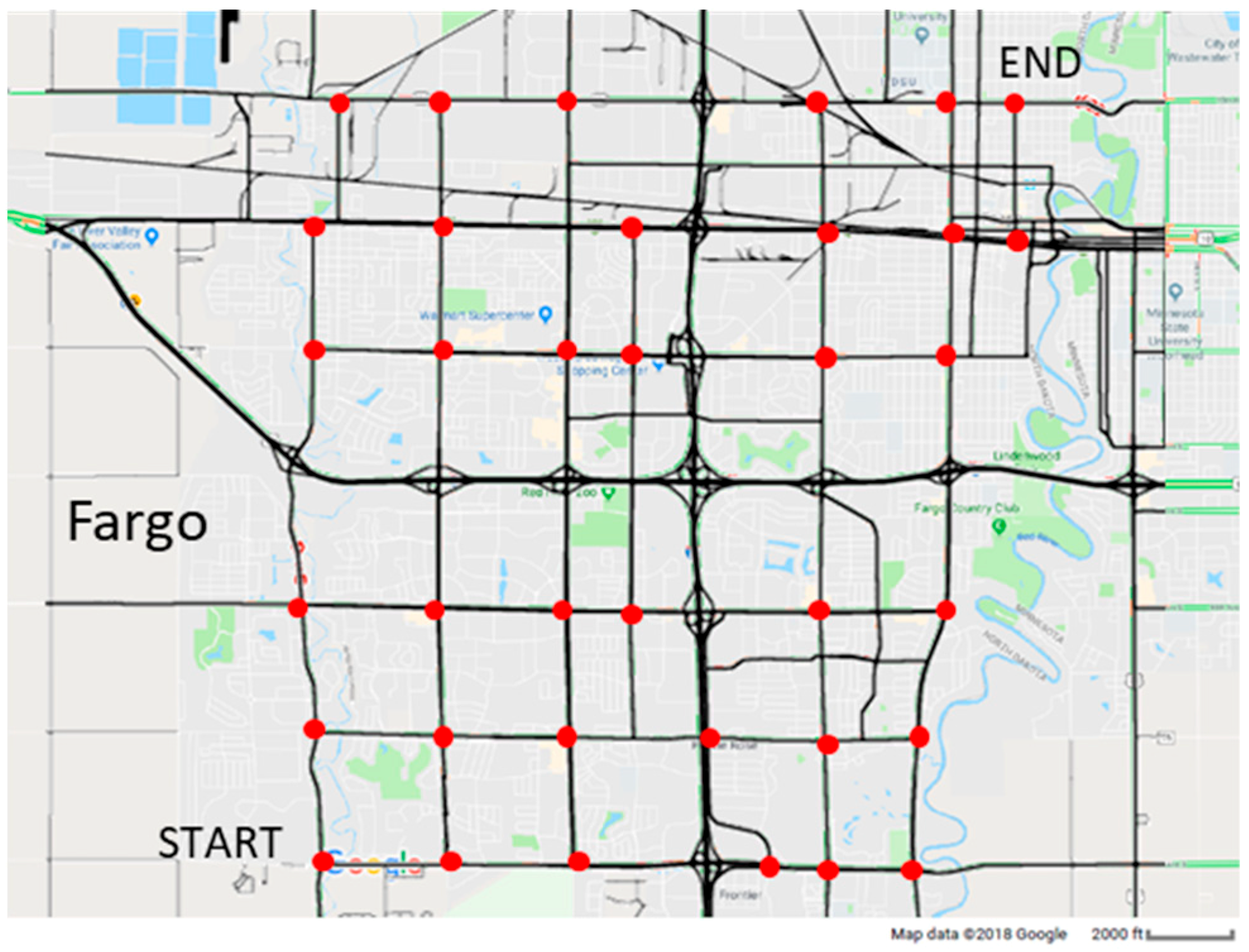
4.1. Case Study Description

Many of the real infrastructure systems, especially supply infrastructure network, are often modeled to resemble lattice networks. Inspired by the water distribution network used in Ref. [37], a lattice network consisting of 36 nodes and 60 edges was considered for this case study. This network used for resilience assessment is shown in Figure 6. The weight of the nodes represents the demand of the nodes. In the case of edges, both the length of each edge and the amount of flow in each edge were considered. The failure was model as a localized attack initiated at a random node and the impact of the attack propagated over time. After the localized attack, eight nodes were isolated randomly to mimic random failure pattern. The eight nodes were isolated one at a time, and 24 edges were also set to ‘randomly damaged’ and removed to result in a region of isolated nodes.

To illustrate the challenges in resilience assessment, there are two critical performance measures considered in this case study, the maximum flow and the shortest path distance from node 1 to node 36 (Figure 7). The maximum flow quantifies the amount of load this network can carry, follows the concept of “the more, the better”. The best route is indicated by the shortest path distance, where it quantified the most efficient route with the least travel distance. Opposite from the maximum flow, the shortest path distance follows the concept of “the least, the better”. The damage scenario resulted in a decrease in the maximum flow from 75 to 48 units, and the shortest path length increases from 192 to 229 units. The transition of network performance from its original state to after attack state is shown in

Table 2. Degradation propagation from original to degraded state.

Time	Critical Performance		Description
	Max flow	Shortest Path
0	75	192	Original state
1 *	75	206	1 node was isolated
2	75	206	2 nodes were isolated
3	75	206	3 nodes were isolated
4	75	229	4 nodes were isolated
5	75	229	5 nodes were isolated
6	75	229	6 nodes were isolated
7	75	229	7 nodes were isolated
8 **	48	229	8 nodes were isolated

* Failure occurred at time step 1 and propagated through time step 8; ** Failure stopped propagating at time step 8.

.

Different stages in the resilience assessment for the water distribution network can be seen in Figure 7. As mentioned in Section 2.2, there are three recovery strategies that are deemed to be appropriate for recovering network that suffers from a localized attack: (1) preferential recovery based on nodal weight (PRNW), (2) periphery recovery (PR), and (3) localized recovery (LR). The effectiveness of these three recovery strategies will be compared against each other with the proposed framework in Section 2.3. As part of this assessment process, an optimized recovery strategy among the three strategies will be selected. It is assumed that the network will recover fully (100%) after implementing any recovery strategy, given that the iteration properties can differ.

In order to determine the best recovery strategy that resulted in the highest resilience metric with the lowest cost, the proposed optimization model was implemented with some predetermined parameters. To measure the resilience level of the system, resilience metric R was used. Among all the above-mentioned infrastructure-related resilience metrics, R was selected due to its relevance on how the equations were derived from this case study. To conduct the assessment of various recovery strategies, the occurrence of the initial attack was set to happen on the first time step. The damage propagation was indicated with the isolation of one node per iterations. The damage propagation stopped at time step 8, and the recovery was set to start immediately at time step 9. The changes in maximum flow and shortest path distance during the damage propagation stage are tabulated in Table 1, and the changes in system performance during the recovery stage are shown in

Table 3. Changes of max flow and shortest path distance during recovery (shaded area indicates that the recovered state was reached).

Time	PRNW **		PR **		LR ***
	Max Flow	Shortest Path	Max Flow	Shortest Path	Max Flow	Shortest Path
9 *	48	229	48	229	75	229
10	48	229	48	229	75	192
11	73	229	48	229	75	192
12	73	229	75	229	75	192
13	73	229	75	215	75	192
14	75	229	75	192	75	192
15	75	215	75	192	75	192
16	75	192	75	192	75	192
17	75	192	75	192	75	192
18	75	192	75	192	75	192
19	75	192	75	192	75	192
20	75	192	75	192	75	192

* Recovery started at time step 9, ** Recovery stops at time step 17—fully recovered state reached, *** Recovery stopped at time step 12—fully recovered state reached.

.

4.2. Multiobjective Optimization

Selecting the most efficient and robust recovery strategies depends on various factors, such as the overall recovery goal, constraints, and available resources. In order to demonstrate this, three different objectives were introduced and analyzed with the three recovery strategies. For multiobjective formulation, all three recovery strategies were considered together. Another objective function combining the three objective functions was employed to solve the proposed multiobjective optimization formulation. The three objective functions formulated in the proposed multiobjective model are described below in the context of the case study:

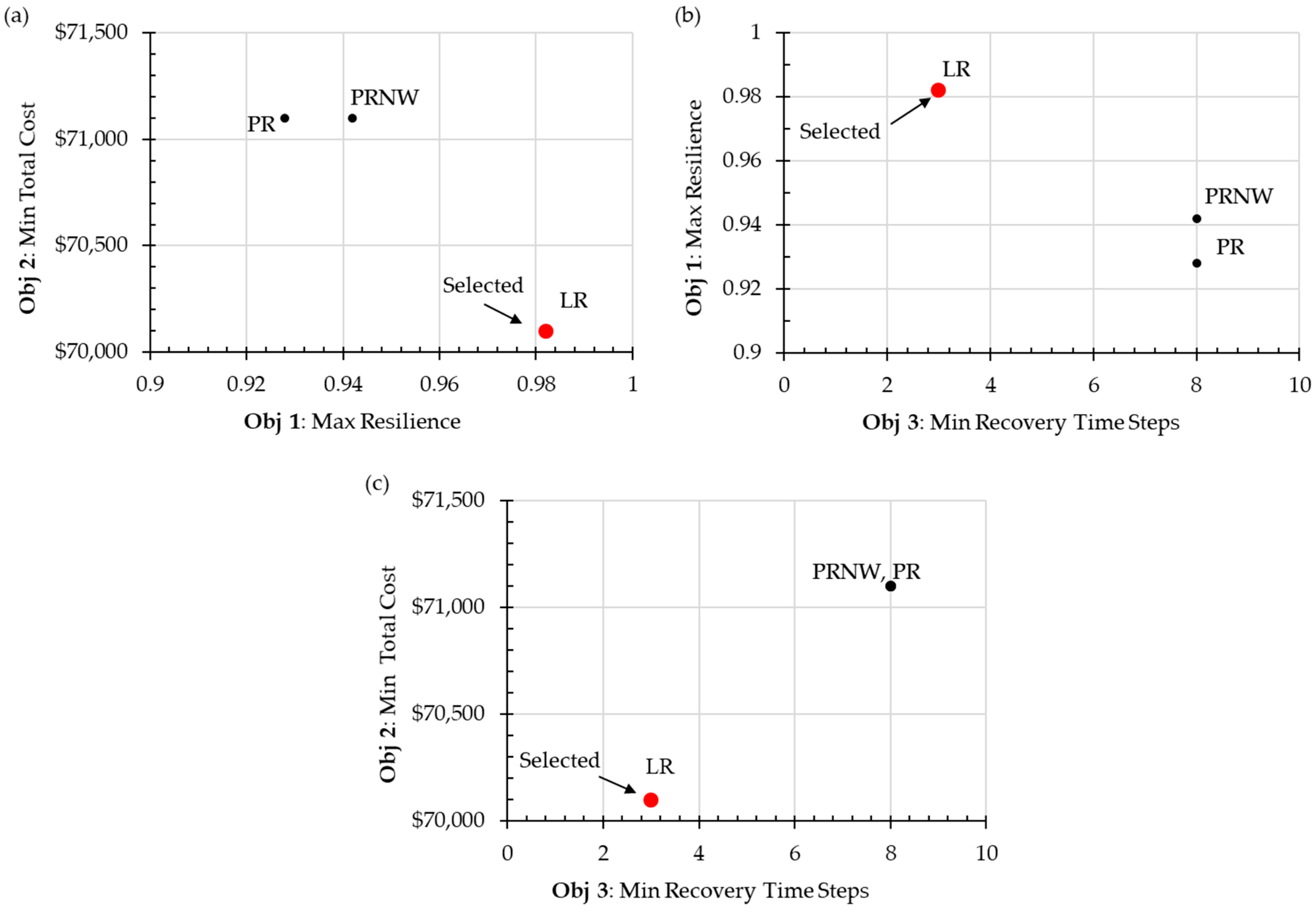
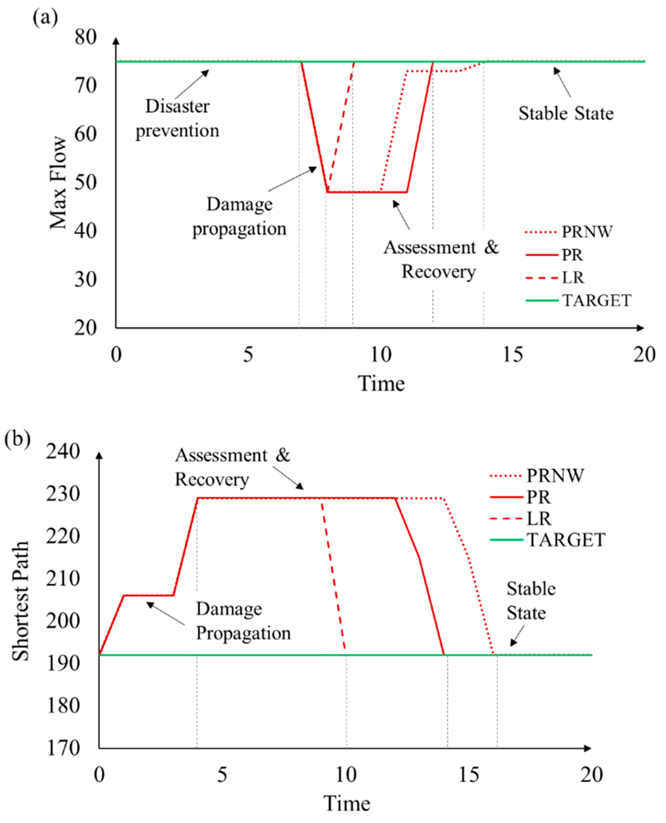
• Objective Function 1: Maximize resilience. The aim of the first objective function is to maximize the overall system resilience by applying the recovery strategy. Here, R was used as the resilience metric. Both maximum flow and the shortest path were considered as the performance measure. For all three recovery strategies, system resilience was quantified, and a recovery strategy was selected based on the highest resilience level.
• Objective Function 2: Minimize cost. The overall recovery cost is minimized by this objective function. For this purpose, the recovery cost at each time step was calculated based on the weight of the edges that need to be recovered. An amount of $200 was assumed to be the fixed cost for each time step of the recovery process. Additionally, the cost of $100 for repairing each unit of edges was added to find the total cost. The strategy with the lowest cost was selected.
• Objective Function 3: Minimize time or number of iterations. Through the third objective function the fastest recovery process was selected (the smallest number of iterations to full recovery).
• Integrated objective: To solve the multiobjective formulation, an integrated objective function, combining Objectives 1–3, is shown in Equation (13).

  $$Minimize-R+C+t_t$$

  (13)

While minimizing Equation (13), the negative value of the resilience is minimized leading to maximizing the actual resilience as well as minimizing the total cost and recovery time. Additionally, all of the objectives were given equal priority while solving the problem.

4.3. Results and Discussion

Each of the three objective functions was analyzed for three different recovery strategies so that the best strategy could be selected based on the main goal of repairing the damaged network. The results of the analysis of each objective function will be discussed respectively in this subsection.

Multiobjective Optimization. To solve the multiobjective model, all three objective functions and the relationship among them were analyzed. The trade-offs between the three objective functions for three recovery strategies were analyzed and are shown in Figure 8a–c. In Figure 8a, the horizontal x-axis represents the resilience which is to be maximized, while the vertical y-axis represents the total cost for the recovery of the network that is to be minimized. It was observed in Figure 8a that, for the resilience values of 0.94, 0.93, and 0.98 for maximum flow performance, the total recovery costs are $71,100, $71,100, and $70,100 for PRNW, PR, and LR, respectively (

Table 4. Resilience assessment of recovery strategies.

	PRNW		PR		LR
	Max Flow	Shortest Path	Max Flow	Shortest Path	Max Flow	Shortest Path
AR	1413	4312	1392	4238	1473	4104
AT	1500	3840	1500	3840	1500	3840
R	0.94	1.12	0.93	1.1	0.98	1.07

and

Table 5. Recovery cost during each recovery step.

Time Steps	Cost ($)
	PRNW	PR	LR
1–8	Damage Propagation Stage
9	7300	7300	42,300
10	4700	7300	24,400
11	13,100	7700	3400
12	3300	8700	0
13	6300	9800	0
14	12,600	4700	0
15	15,100	10,000	0
16	8,700	15,600	0
Total	71,100	71,100	70,100

). It is obvious from Figure 8a that the strategies that should be selected should have the highest resilience value with the minimum total cost. Thus, in this trade-off scenario, LR is deemed to be the most effective strategy and should be selected.

In Figure 8b, the trade-off between recovery time steps and the resilience is shown. In this scenario, the x-axis represents the time steps to be minimized, while the y-axis represents the resilience which is to be maximized. Total recovery time steps 8, 8, and 3 were obtained which is associated with resilience values of 0.94, 0.93, and 0.98 for maximum flow performance for PRNW, PR, and LR, respectively (Table 3 and Table 4). It is observed that higher resilience is associated with lower recovery time. Thus, the most beneficial recovery strategies should be able to recover the network’s function with the least amount of time and cost. In this trade-off scenario, LR should be selected.

Another trade-off between the recovery time steps and the cost is shown in Figure 8c. The x-axis represents the time steps, while the y-axis represents the total recovery cost; both are aimed to be minimized. Total recovery time steps obtained for PRNW, PR, and LR are 8, 8, and 3, respectively, which are associated with the total recovery costs of $71,100, $71,100, and $70,100. As the value of recovery time step and the cost is equal for both PRNW and PR, two of the same data points were obtained and overlapped in Figure 8c. It is observed that the recovery cost is time-dependent, which further means that the total recovery cost increases with the prolonged recovery period. For this trade-off scenario, LR exhibited the fastest recovery with the least total recovery cost among the three recovery strategies and thus should be selected.

From the above-discussed trade-offs analysis, it is observed that all three objective functions are interrelated and their effects should be taken into the decision-making process. Considering the results of the multiobjective optimization, LR should be selected. Because the LR process satisfies all three objective functions, with maximum resilience values 0.98 maximum flow, minimum recovery cost of $70,100, and minimum recovery time steps of 3, LR can be further deemed to be the more superior when compared to PR and PRNW in this case studies. Additional results and further discussion for each objective function are discussed in the following paragraphs.

Analysis of Resilience. After the occurrence of any kind of failures, the overall system performance degrades. If the main aim of repairing the damaged network is retrieving the highest possible percentage of initial network performance, it also refers to achieving the highest system resilience. Here resilience metric R (see Equation (1)) was used, which is quantified based on the ratio of the area below the targeted performance curve and the real curve. The resulting resilience curves after applying all three recovery strategies are shown in Figure 9a for maximum flow, and Figure 9b for the shortest path.

The results of resilience assessment of recovery strategies are summarized in Table 4. A_R and A_T refer to the area under the real performance curve and the area under the targeted performance curve respectively. With maximum flow, the A_R values are 1413, 1392, and 1473 for PRNW, PR, and LR, respectively, and the A_T value is 1500. It is shown that A_R is always lesser than A_T resulting in resilience values of 0.94, 0.93, and 0.98 for PRNW, PR, and LR, respectively. This indicates that LR shows the highest resilience as the maximum flow follows ‘the larger the better’ concept. On the other hand, with shortest path A_R values are 4312, 4238, and 4104 for PRNW, PR, and LR, respectively, and the A_T value is 3840. A_R is always greater than A_T, resulting in resilience values of 1.12, 1.1, and 1.07. As the shortest path follows “the smaller, the better” concept, LR is the most resilient strategy in this case as well.

Analysis of Cost. While aiming to achieve the highest system resilience, the repairing cost should also be considered. This is because, in real cases, there are always budget constraints that may limit the recovery process in various ways. It should be noted that the recovery strategy with the lowest cost should be selected while considering system resilience. The results found from cost analysis are summarized in Table 5.

From Table 5, it is observed that the total recovery cost for PRNW is $71,100; PR is $71,100, and LR is $70,100, indicating that LR should be selected here. However, in the initial two steps the recovery cost for LR are $42,300 and $24,400, for PRNW are $7300 and $4700, and for PR are $7300 and $7300. This indicates that LR costs more in initial steps compared to the other two strategies. In the real case, these initial higher costs may exceed the budget resulting in the selection of a different recovery strategy, although the overall cost for LR is lower. The changes in costs in each time step can be compared with the cost vs. time graph given in Figure 10.

Analysis of Time. While aiming for highest system resilience, faster recovery is also necessary along with recovery cost, because, in reality, immediate recovery is needed after any disaster and, also, it contributes to system resilience. Considering these facts, the recovery strategies were evaluated based on the time or the number of time steps needed for a full recovery scenario and the restoration sequence. The results found are summarized in

Table 6. Iteration details of recovery strategies.

Time Step	PRNW		PR		LR
	Recovered Edges *	Sum of Weights	Recovered Edges *	Sum of Weights	Recovered Edges *	Sum of Weights
9	23, 15	71	23, 15	71	28, 36, 38, 39, 25, 27, 26, 30, 37, 47, 41, 49	421
10	26, 36	45	40, 41	71	14, 16, 15, 17, 19, 23, 29, 34, 40, 50	242
11	38, 40, 41	129	26, 34, 37	75	6	32
12	34, 37	31	47, 49, 50	85
13	25, 28	61	6, 14, 16	96
14	39, 47, 49, 50	124	19, 29, 30	45
15	6, 14, 16, 17	149	36, 38, 39	98
16	19, 27, 29, 30	85	17, 25, 27, 28	154
17–20	Stable State

* Restoration sequence was sorted from the first to the last node restored.

. It is observed that PRNW and PR are able to recover all the damaged edges in time step 17 and LR in time step 12. PRNW and PR took 8 time steps to reach a fully connected network, while LR requires only 3 time steps. Further, from Table 3, it is also observed that the water supply infrastructure network system performances, maximum flow or shortest path, were able to be restored earlier, although the network was not fully connected. The maximum flow for PRNW was restored at time step 14, and the shortest distance was restored at time step 16 while the whole network was fully connected at time step 17. Although PR needed the same amount of time step to fully reconnect the network, the maximum flow based on PR was restored at time step 12 and the shortest path performance at time step 14. Considering only the restoration of the individual performance, PR can be claimed to recover faster than the PRNW. In addition, LR managed to recover the network’s maximum flow and shortest path at time step 9 and 10, respectively. From the results of the number of time steps required to reach a full recovery after a localized attack, LR would be a much faster process compared to PRNW and PR strategies. Although not as immediate as LR, PRNW and PR are two recovery strategies that are quite effective for postdisaster recovery in a short time. Because of their low computational complexity, it is easy to employ PRNW and PR immediately.

Considering the results, it is clear that the LR process should be selected from the perspective of all three objectives. However, if the initial cost of recovery is needed to be kept in the lower range, PRNW or PR would be more appropriate. In addition to the presented work, there are some challenges that are needed to be addressed in the future work of this study. To minimize the complexity in measuring system resilience, a standard for selecting a resilience metric for the application of infrastructure systems should be agreed upon. The trade-offs between different constraints could be analyzed with a larger network to achieve a more realistic result, which will be addressed in future work. In addition, uncertainties during implementation should be considered in the preliminary assessment to ensure the probability of successful implementation. Further, the time dependence dynamic behavior of the network could be another challenging area that needs to be investigated. A time-dependent optimized restoration is crucial to consider the goal of the recovery at a given time period after a disaster occurred. To address this challenge, a time-dependent dynamic optimization of network resilience for selecting recovery strategies in different stages will be investigated. Localized attacks may affect several critical local nodes; this research could further expand to include local node analysis for more robust operation. It is possible that a recovery strategy might perform better for a particular type of disruption. The proposed approach can be expanded in the future to accommodate multiple disruption types. A multiobjective-based restoration for multiple disruptions over time will be formulated for future analysis.

5. Conclusions

In this paper, a small initiative was taken to conduct a resilience assessment of infrastructure networks under localized attacks. The resilience assessment was conducted with the implementation of various recovery strategies that have been deemed effective in recovering a network after localized attacks. A comparison framework equipped with multiobjective formulations is proposed with the goal of identifying the most effective recovery strategy among a selection of visible strategies that can be eventually implemented. A case study of a water distribution network restoration after a localized attack was employed in this paper. The case study was assessed with three recovery strategies: preferential recovery based on nodal weight (PRNW), periphery recovery (PR), and localized recovery (LR). In addition, a multiobjective optimization model was also developed in order to find the optimum resilience-based recovery strategy. This multiobjective formulation aims to maximize the system’s resilience while minimizing both recovery cost and time. To show the relationship between the objective functions, three trade-offs between the combination two functions were presented. The case study results show that the localized recovery strategy has the ability to achieve the highest system resilience within the shortest recovery time with the lowest cost. It can be further interpreted that LR was superior among the three recovery strategies for this particular network situation when subjected to a localized attack scenario.

Based on the case study results for a localized attack scenario, restoration efforts should be directed towards restoring more links to bridge the isolated nodes. Resilience in a broader term is associated with time and cost. Higher resilience value is attributed to a faster recovery, while faster recovery may require more cost in terms of resources. On the other hand, there are typically associated with fixed costs and variable costs in every recovery strategy. A longer recovery period may incur higher costs at the end of the recovery period. This scenario may also lead to lower resilience value. However, this type of recovery typically required lesser resources at the beginning when compared with a faster recovery strategy. The proposed resilience-based recovery assessment can be employed as a baseline methodology to evaluate the effectiveness of various recovery strategies, and can be easily implemented, modified, or replicated to fit the application of interest by other researchers or practitioners. Along with a global approach for assessing recovery strategies, the obtained results give an insight into future research directions in this field, such as incorporating multiple disaster occurrences in the multiobjective formulation and the development of a time-dependent dynamic optimized recovery strategy.

References

1. Bocchini, P.; Frangopol, D.M.; Ummenhofer, T.; Zinke, T. Resilience and sustainability of civil infrastructure: Toward a unified approach. J. Infrastruct. Syst. 2013, 20, 04014004. [Google Scholar] [CrossRef]
2. Mattsson, L.-G.; Jenelius, E. Vulnerability and resilience of transport systems—A discussion of recent research. Transp. Res. Part A Policy Pract. 2015, 81, 16–34. [Google Scholar] [CrossRef]
3. Hu, F.; Yeung, C.H.; Yang, S.; Wang, W.; Zeng, A. Recovery of infrastructure networks after localized attacks. Sci. Rep. 2016, 6, 24522. [Google Scholar] [CrossRef] [PubMed]
4. Linkov, I.; Bridges, T.; Creutzig, F.; Decker, J.; Fox-Lent, C.; Kröger, W.; Lambert, J.H.; Levermann, A.; Montreuil, B.; Nathwani, J.; et al. Changing the resilience paradigm. Nat. Clim. Change 2014, 4, 407. [Google Scholar] [CrossRef]
5. Ganin, A.A.; Kitsak, M.; Marchese, D.; Keisler, J.M.; Seager, T.; Linkov, I. Resilience and efficiency in transportation networks. Sci. Adv. 2017, 3, e1701079. [Google Scholar] [CrossRef] [PubMed] [Green Version]
6. Adams, T.M.; Bekkem, K.R.; Toledo-Durán, E.J. Freight resilience measures. J. Transp. Eng. 2012, 138, 1403–1409. [Google Scholar] [CrossRef]
7. Uday, P.; Marais, K. Designing resilient systems-of-systems: A survey of metrics, methods, and challenges. Syst. Eng. 2015, 18, 491–510. [Google Scholar] [CrossRef]
8. Yodo, N.; Wang, P. A control-guided failure restoration framework for the design of resilient engineering systems. Reliab. Eng. Syst. Saf. 2018, 178, 179–190. [Google Scholar] [CrossRef]
9. Ouyang, M.; Dueñas-Osorio, L.; Min, X. A three-stage resilience analysis framework for urban infrastructure systems. Struct. Saf. 2012, 36, 23–31. [Google Scholar] [CrossRef]
10. Whitson, J.C.; Ramirez-Marquez, J.E. Resiliency as a component importance measure in network reliability. Reliab. Eng. Syst. Saf. 2009, 94, 1685–1693. [Google Scholar] [CrossRef]
11. Yodo, N.; Wang, P. Engineering resilience quantification and system design implications: A literature survey. J. Mech. Design 2016, 138, 1–13. [Google Scholar] [CrossRef]
12. Aydin, N.Y.; Duzgun, H.S.; Heinimann, H.R.; Wenzel, F.; Gnyawali, K.R. Framework for improving the resilience and recovery of transportation networks under geohazard risks. Int. J. Disaster Risk Reduct. 2018, 31, 832–843. [Google Scholar] [CrossRef]
13. Cox, A.; Prager, F.; Rose, A. Transportation security and the role of resilience: A foundation for operational metrics. Transp. Policy 2011, 18, 307–317. [Google Scholar] [CrossRef]
14. Wang, J.; Muddada, R.R.; Wang, H.; Ding, J.; Lin, Y.; Liu, C.; Zhang, W. Toward a resilient holistic supply chain network system: Concept, review and future direction. IEEE Syst. J. 2016, 10, 410–421. [Google Scholar] [CrossRef]
15. Munoz, A.; Dunbar, M. On the quantification of operational supply chain resilience. Int. J. Prod. Res. 2015, 53, 6736–6751. [Google Scholar] [CrossRef]
16. Yodo, N.; Wang, P. Resilience analysis for complex supply chain systems using bayesian betworks. In Proceedings of the 54th AIAA Aerospace Sciences Meeting, San Diego, CA, USA, 4–8 January 2016; p. 0474. [Google Scholar]
17. Attoh-Okine, N.O.; Cooper, A.T.; Mensah, S.A. Formulation of resilience index of urban infrastructure using belief functions. IEEE Syst. J. 2009, 3, 147–153. [Google Scholar] [CrossRef]
18. Borsekova, K.; Nijkamp, P.; Guevara, P. Urban resilience patterns after an external shock: An exploratory study. Int. J. Disaster Risk Reduct. 2018, 31, 381–392. [Google Scholar] [CrossRef]
19. Wang, J.; Liu, H. Snow removal resource location and allocation optimization for urban road network recovery: A resilience perspective. J. Ambient Intell. Humaniz. Comput. 2018, 10, 395–408. [Google Scholar] [CrossRef]
20. Murray-Tuite, P.M. A comparison of transportation network resilience under simulated system optimum and user equilibrium conditions. In Proceedings of the 2006 Winter Simulation Conference, Monterey, CA, USA, 3–6 December 2006; pp. 1398–1405. [Google Scholar]
21. Dong, Y.; Frangopol, D.M. Risk and resilience assessment of bridges under mainshock and aftershocks incorporating uncertainties. Eng. Struct. 2015, 83, 198–208. [Google Scholar] [CrossRef]
22. Zorn, C.R.; Shamseldin, A.Y. Post-disaster infrastructure restoration: A comparison of events for future planning. Int. J. Disaster Risk Reduct. 2015, 13, 158–166. [Google Scholar] [CrossRef]
23. Liao, T.-Y.; Hu, T.-Y.; Ko, Y.-N. A resilience optimization model for transportation networks under disasters. Nat. Hazards 2018, 93, 469–489. [Google Scholar] [CrossRef]
24. Losada, C.; Scaparra, M.P.; O’Hanley, J.R. Optimizing system resilience: A facility protection model with recovery time. Eur. J. Oper. Res. 2012, 217, 519–530. [Google Scholar] [CrossRef]
25. Turnquist, M.; Vugrin, E. Design for resilience in infrastructure distribution networks. Environ. Syst. Decis. 2013, 33, 104–120. [Google Scholar] [CrossRef] [Green Version]
26. Figueroa-Candia, M.; Felder, F.A.; Coit, D.W. Resiliency-based optimization of restoration policies for electric power distribution systems. Electr. Power Syst. Res. 2018, 161, 188–198. [Google Scholar] [CrossRef]
27. Margolis, J.T.; Sullivan, K.M.; Mason, S.J.; Magagnotti, M. A multi-objective optimization model for designing resilient supply chain networks. Int. J. Prodt. Econ. 2018, 204, 174–185. [Google Scholar] [CrossRef]
28. Almoghathawi, Y.; Barker, K.; Albert, L.A. Resilience-driven restoration model for interdependent infrastructure networks. Reliab. Eng. Syst. Saf. 2019, 185, 12–23. [Google Scholar] [CrossRef]
29. Fang, Y.-P.; Sansavini, G. Optimum post-disruption restoration under uncertainty for enhancing critical infrastructure resilience. Reliab. Eng. Syst. Saf. 2019, 185, 1–11. [Google Scholar] [CrossRef]
30. Ouyang, M. Critical location identification and vulnerability analysis of interdependent infrastructure systems under spatially localized attacks. Reliab. Eng. Syst. Saf. 2016, 154, 106–116. [Google Scholar] [CrossRef]
31. Mathias, J.-D.; Clark, S.; Onat, N.; Seager, T. An integrated dynamical modeling perspective for infrastructure resilience. Infrastructures 2018, 3, 11. [Google Scholar] [CrossRef]
32. Alderson, D.L.; Brown, G.G.; Carlyle, W.M.; Cox, L.A., Jr. Sometimes there is no “most-vital” arc: Assessing and improving the operational resilience of systems. Mil. Oper. Res. 2013, 18, 21–37. [Google Scholar] [CrossRef]
33. Alderson, D.L.; Brown, G.G.; Carlyle, W.M. Operational models of infrastructure resilience. Risk Anal. 2015, 35, 562–586. [Google Scholar] [CrossRef]
34. Alderson, D.L.; Brown, G.G.; Carlyle, W.M.; Wood, R.K. Assessing and improving the operational resilience of a large highway infrastructure system to worst-case losses. Transp. Sci. 2017, 52, 1012–1034. [Google Scholar] [CrossRef]
35. Shang, Y. Localized recovery of complex networks against failure. Sci. Rep. 2016, 6, 30521. [Google Scholar] [CrossRef] [Green Version]
36. Bruneau, M.; Chang, S.E.; Eguchi, R.T.; Lee, G.C.; O’Rourke, T.D.; Reinhorn, A.M.; Shinozuka, M.; Tierney, K.; Wallace, W.A.; Winterfeldt, D.V. A framework to quantitatively assess and enhance the seismic resilience of communities. Earthq. Spectra 2003, 19, 733–752. [Google Scholar] [CrossRef]
37. Creaco, E.; Franchini, M.; Alvisi, S. Optimal placement of isolation valves in water distribution systems based on valve cost and weighted average demand shortfall. Water Resour. Manag. 2010, 24, 4317–4338. [Google Scholar] [CrossRef]
Figure 1. A typical aftermath of localized attacks [3].
Infrastructures 04 00011 g001
Figure 2. The illustration of various strategic repair processes after a localized attack on a two-dimensional square lattice network with heterogeneously populated nodes [3,35].
Infrastructures 04 00011 g002
Figure 3. General resilience-based recovery assessment framework.
Infrastructures 04 00011 g003
Figure 4. Aspects of resilience [1,36].
Infrastructures 04 00011 g004
Figure 5. Performance process of an infrastructure system during disruptive events [15].
Infrastructures 04 00011 g005
Figure 6. A water distribution network case study.
Infrastructures 04 00011 g006
Figure 7. The assessment model in different stages of resilience.
Infrastructures 04 00011 g007
Figure 8. Objective trade-offs between (a) total recovery cost and resilience, (b) total recovery cost and recovery time steps, and (c) resilience and recovery time steps.
Infrastructures 04 00011 g008
Figure 9. Resilience curve based on (a) maximum flow and (b) shortest path.
Infrastructures 04 00011 g009
Figure 10. Changes in recovery cost in each time step.
Infrastructures 04 00011 g010